How Large is the “Natural” Magnetic Moment?

The “natural” magnetic moment of a particle of spin $S$ is generally assumed to be that given by the Belinfante conjecture and has the value $g=1/S$ for its gyromagnetic ratio. Thus, for the spin 1/2 electron we find the Dirac value $g_{\rm e}=2$. However, in the standard model the charged W boson, a spin one particle, is found to have the value $g_{W^{+}}=2$. We show how this result comes about and argue that the “natural” value for any particle of spin S should be $g=2$, independent of spin.

1 Introduction

One of the great successes of Dirac theory is the prediction of the magnetic moment of the electron. Usually this is written in terms of the gyromagnetic ratio or g-factor, which is defined via the relation

$$\vec{\mu}={eg\over 2m}\vec{S}$$ (1)

where $\vec{\mu}$ represents the magnetic moment of a particle of mass $m$, charge $e$, and spin $\vec{S}$. Then for spin 1/2 the simple Dirac theory makes the prediction $g=2$, which is the value found experimentally (except for very small corrections from photon loop effects) for the electron, as well as for its standard model partners $\mu$ and $\tau$[1]. Feynman argued that the value $g=2$ could be generated in an intuitive fashion by generalizing the Schrödinger equation for a spin 0 system of mass $m$ and charge $e$ interacting with an external vector potential $A^{\mu}=(\phi,\vec{A})$—

$$i{\partial\over\partial t}\psi=\left({(-i\vec{\nabla}-e\vec{A})^{2}\over 2m}+e\phi\right)\psi$$ (2)

to the form

$$i{\partial\over\partial t}\psi=\left({1\over 2m}\vec{\sigma}\cdot(-i\vec{\nabla}-e\vec{A})\vec{\sigma}\cdot(-i\vec{\nabla}-e\vec{A})+e\phi\right)\psi$$ (3)

in the case of spin 1/2[2]. Using the Pauli matrix identity

$$\sigma_{i}\sigma_{j}=\delta_{ij}+i\epsilon_{ijk}\sigma_{k}$$ (4)

the spin 1/2 Schrödinger equation can be written in the alternative form

$$i{\partial\over\partial t}\psi=\left({(-i\vec{\nabla}-e\vec{A})^{2}\over 2m}-{e\over 2m}\vec{\sigma}\cdot\vec{\nabla}\times\vec{A}+e\phi\right)\psi$$ (5)

wherein the Hamiltonian is that of the simple spinless system accompanied by a magnetic moment interaction with g=2.

Of course, for charged spin 1/2 systems other than the $e,\mu,\tau$, e.g., the proton or neutron, there exist large deviations from the Dirac value—$g_{\rm p}=5.58,\,\,g_{\rm n}=-3.82$ on account of loop effects associated with the strong interactions[3]. However, these are not fundamental systems, but rather are bound states of constituent quarks.

It is then an interesting question to ask whether there is a corresponding “natural” value for the g-factor of fundamental systems having spin other than 1/2. One answer to this question was given long ago by Belinfante, who evaluated the magnetic moment of a simple spin 3/2 system and observed that the g-factor was 2/3. Combining this with known results for Dirac (spin 1/2) and Proca (spin 1) systems for which the g-factors are 2 and 1 respectively, Belinfante proposed that for a system of spin $S$, $g_{S}=1/S$[4], and this has become known as the Belinfante conjecture. This result was proven for arbitrary spin by Case and others nearly five decades ago[5] and more recently by Hagen and Hurley[6] and is based on the assumption that the interaction of the spinning system with the electromagnetic field is generated by the simple “minimal substitution”[8]—

$$i\nabla_{\mu}\longrightarrow\pi_{\mu}\equiv i\nabla_{\mu}-eA_{\mu}$$ (6)

that is known from classical electrodynamics to generate the interactions of a charged particle with an external vector potential[7]. However, in order to check Belinfante’s proposal, we are limited by the fact that the only other manifestations of charged particles which do not interact strongly are the $W^{\pm}$ bosons, which have unit spin and therefore would be expected to have $g_{W}^{\rm Belinfante}=1$. In the tree level standard model, however, the charged W-boson is found to have $g_{W}^{\rm exp}=2$, due to the requirement that it is also a gauge boson for the electroweak interaction[9]. Below we shall show how this feature comes about and will argue that in fact the “natural” value for the g-factor of a fundamental system of spin $S$ is $g_{S}=2$—independent of $S$!. This is not a new suggestion, and rather has been reached by a number of authors in recent years. In particular the work of Ferrara, Porrati, and Telegdi shows that Compton scattering from targets of mass $m$ and arbitrary spin violates unitarity at photon energy $\omega_{i}\sim m$ unless $g_{S}=2$[10], while for those readers looking for a broad and very interesting historical summary as well as some of the constraints posed by general relativity, the article by Pfister and King is required reading[11]. We shall give below a more limited set of arguments, which, however, we believe are more than enough to buttress the case.

In the next section then we review how the g-factor can be identified in a given relativistic Lagrangian, using the cases of spin 1/2 and spin 1 as examples. (An alternative approach, based on a nonrelativistic reduction, is presented in the Appendix.) In section 3 we demonstrate why the charged W-boson has a g-factor which differs from that suggested by Belinfante and cite specific arguments why one might expect the prediction $g=2$ to be generally valid for systems of arbitrary spin. Finally, we summarize our results in a brief concluding section.

2 The Belinfante Conjecture

In order to motivate the Belinfante conjecture, we need to see how to extract the g-factor from a given relativistic Lagrangian. This can be done in a number of ways. A standard method is to use a nonrelativistic reduction, as demonstrated in the Appendix. However, one can also identify the g-factor directly by isolating the magnetic interaction in the Lagrangian, as we show here. We begin by reviewing how the Dirac value—$g=2$—arises for spin 1/2.

2.1 S=1/2

The well-known Dirac Lagrangian for a free spin 1/2 particle is

$${\cal L}=\bar{\psi}(x)(i\not\!{\nabla}-m)\psi(x)$$ (7)

Making the minimal substitution—Eq. 6—this becomes for the case of a charged system

$${\cal L}=\bar{\psi}(x)(i\not\!{\nabla}-e\not\!\!{A}-m)\psi(x)$$ (8)

and we can identify the interaction Lagrangian by picking out the piece of the Lagrangian proportional to $A^{\mu}$

$${\cal L}_{\rm int}=-eA^{\mu}(x)\bar{\psi}(x)\gamma_{\mu}\psi(x)$$ (9)

By use of the free Dirac equation for the fields

$$\psi(x)={i\over m}\not\!{\nabla}\psi(x)$$ (10)

Eq. 9 can be rewritten as

$${\cal L}_{\rm int}={ie\over 2m}A^{\mu}\left[\bar{\psi}\gamma_{\mu}\gamma_{\nu}\nabla^{\nu}\psi-(\nabla^{\nu}\bar{\psi})\gamma_{\nu}\gamma_{\mu}\psi\right]$$ (11)

Then using the matrix identity

$$\gamma_{\mu}\gamma_{\nu}=\eta_{\mu\nu}-i\sigma_{\mu\nu}$$ (12)

the interaction Lagrangian may be written in the so-called Gordon form as[8]

$${\cal L}_{\rm int}={e\over 2m}A^{\mu}(x)\bar{\psi}(x)i\overleftrightarrow{\nabla}_{\mu}\psi(x)+{e\over 2m}A^{\mu}(x)\nabla^{\nu}(\bar{\psi}(x)\sigma_{\mu\nu}\psi(x))$$ (13)

where we have defined

$$D(x)\overleftrightarrow{\nabla}_{\mu}F(x)\equiv D(x)\nabla_{\mu}F(x)-(\nabla_{\mu}D(x))F(x)$$

The first component of Eq. 13 is a convective term which is not of interest to our present focus. Rather we examine the second term, which involves the total derivative, and observe that it can be rewritten in the form

$${\cal L}_{\rm int}=-{e\over 4m}F^{\mu\nu}\psi(x)\sigma_{\mu\nu}\psi(x)$$ (14)

where we have integrated by parts and used the fact that $\sigma_{\mu\nu}$ is antisymmetric in the indices $\mu\nu$. Finally, noting that $F^{ij}=-\epsilon_{ij\ell}B^{\ell}$ and $\sigma_{ij}=2\epsilon_{ijk}S_{k}$, where

$$\vec{S}=\left(\begin{array}[]{cc}{1\over 2}\vec{\sigma}&0\\ 0&{1\over 2}\vec{\sigma}\end{array}\right)$$

is the spin operator, we isolate the magnetic interaction—

$${\cal L}_{\rm mag}={e\over m}\bar{\psi}(x)\vec{S}\cdot\vec{B}\psi(x)$$ (15)

and read off the well-known result $g=2$.

Of course, this prediction is not expected to be exact. In the case of the electron, photon loops make small ${\cal O}(\alpha)$ corrections, while, in the case of the proton, strong interaction corrections yield large modifications of ${\cal O}(1)$. Such corrections, usually called the “anomalous” magnetic moment—$\kappa$—can be accounted for phenomenologically by inclusion of a so-called Pauli term in the Dirac equation[13]—

$$(i\not\!{\nabla}-e\not\!\!{A}-{e\kappa\over 2m}\sigma_{\mu\nu}F^{\mu\nu}-m)\psi(x)=0$$ (16)

As mentioned above, it has been proven rigorously that, for arbitrary spin, inclusion of the electromagnetic interaction by the minimal substitution yields the “natural” value for the magnetic moment given by the Belinfante conjecture[5]. The proofs are rather formal, and we eschew the temptation to reproduce them here. Rather we shall examine only the case of unit spin, in order to demonstrate how higher spins are handled. This is an important case, however, because there exists a fundamental charged particle that is analogous to the electron in that it does not participate in the strong interactions and therefore may be expected to carry its “natural” value of the magnetic moment. This is the charged W-boson, which is the carrier of the weak interaction, and can be used to check of these ideas. Before discussing the $W^{\pm}$, however, we demonstrate how the minimal prediction for a spin one magnetic moment comes about.

2.2 Spin 1

The Lagrangian which describes a free neutral spin one system is that given by Proca[14]

$${\cal L}={1\over 2}B^{\alpha}(x)[\eta_{\alpha\beta}(\Box+m^{2})-\nabla_{\beta}\nabla_{\alpha}]B^{\beta}(x)$$ (17)

and in the case of a spin 1 particle which is charged, we can introduce the electromagnetic interaction as before by making the minimal substitution—

$${\cal L}=B^{\alpha\dagger}(x)[\eta_{\alpha\beta}((\nabla+ieA)^{\mu}(\nabla+ieA)_{\mu}+m^{2})-(\nabla+ieA)_{\beta}(\nabla+ieA)_{\alpha}))]B^{\beta}(x)$$ (18)

We isolate the single photon piece of the interaction Lagrangian—

$${\cal L}_{\rm int}=ieA^{\mu}(x)B^{\alpha\dagger}(x)[\eta_{\alpha\beta}\overleftrightarrow{\nabla}_{\mu}-\eta_{\beta\mu}\nabla_{\alpha}]B^{\beta}(x)-\eta_{\alpha\mu}(\nabla_{\beta}B^{\alpha\dagger}(x))B^{\beta}(x)$$ (19)

which, as before, can be rewritten as a linear combination of total derivative and $\overleftrightarrow{\nabla}$ pieces as

$${\cal L}_{\rm int} = ieA^{\mu}B^{\alpha\dagger}(x)[\eta_{\alpha\beta}\overleftrightarrow{\nabla}_{\mu}+{1\over 2}\eta_{\mu\beta}\overleftrightarrow{\nabla}_{\alpha}+{1\over 2}\eta_{\mu\alpha}\overleftrightarrow{\nabla}_{\beta}]B^{\beta}(x)$$ (20)

$$+ {ie\over 2}(\eta_{\mu\beta}\nabla_{\alpha}-\eta_{\mu\beta}\nabla_{\alpha})(B^{\alpha\dagger}(x)B^{\beta}(x))$$

Neglecting the convective component, we focus on the total derivative term, which, integrating by parts, assumes the form

$${\cal L}_{\rm int}(x)=-{ie\over 2}F^{\mu\nu}(x)(B_{\nu}^{\dagger}(x)B_{\mu}(x)-B_{\mu}^{\dagger}(x)B_{\nu}(x))$$ (21)

Defining matrix elements of the spin operator via[17]

$$B^{\dagger}_{i}B_{j}-B^{\dagger}_{j}B_{i}=-i\epsilon_{ijk}<f|S_{k}|i>$$ (22)

the interaction Lagrangian becomes

$${\cal L}_{\rm int}=e\vec{B}\cdot<f|\vec{S}|i>$$ (23)

Finally, dividing by the factor 2m, which accounts for the normalization of the unit spin states, we find the Belinfante result for the g-factor—$g_{S=1}=1$.

2.3 Charged W-Boson

As discussed above, the electron magnetic moment agrees with its “natural” value given by the Belinfante conjecture up to small terms due to photon loop corrections, but how about the charged W-boson, which is the unit-spin analog of the electron in that there can be no strong interaction corrections? From Eq. 23, we would expect a g-factor having the value unity, but in the tree level standard model the correct number is predicted to be twice this value, and this prediction is confirmed experimentally—$g_{W^{\pm}}=2.20\pm 0.20$[16]. What is going on, and why is such a large shift to be expected?

The answer can be found in the simple Lagrangian which describes the charged W and the requirement that it be a Yang-Mills field—i.e., that the electroweak interaction is a gauge theory[9]. This means that the spin one Lagrangian which contains the charged-W has the Proca form—

$${\cal L}=-{1\over 4}(\vec{U}_{\mu\nu})^{2}+{m^{2}\over 2}\vec{U}_{\mu}^{2}$$ (24)

but the SU(2) field tensor $\vec{U}_{\mu\nu}$ contains an additional term on account of the required gauge invariance[9]

$$\vec{U}_{\mu\nu}=\pi_{\mu}\vec{U}_{\nu}-\pi_{\nu}\vec{U}_{\mu}-ig\vec{U}_{\mu}\times\vec{U}_{\nu}$$ (25)

where $g$ is the SU(2) electroweak coupling constant. This “extra” term in the field tensor is responsible for the interactions involving three and four W-bosons. For our purpose, however, we pick out only the term involving a pair of charged W-bosons

$${\cal L}_{WW} = -{1\over 2}W^{+\dagger}_{\mu\nu}W^{+\mu\nu}-{1\over 2}W^{-\dagger}_{\mu\nu}W^{-\mu\nu}+{m^{2}\over 2}(W^{+\dagger}_{\mu}W^{+\mu}+W^{-\dagger}_{\mu}W^{-\mu})$$ (26)

$$- gW^{0\mu\nu}(W^{+\dagger}_{\mu}W^{+}_{\nu}-W^{-\dagger}_{\mu}W^{-}_{\nu})$$

where here the field tensors involving the W-boson are of the simple form

$$W_{\mu\nu}=\pi_{\mu}W_{\nu}-\pi_{\nu}W_{\mu}$$

We see that there appears to be an additional triple-W coupling. However, this is illusory. In the standard model there is no neutral W-boson. Rather the field $W^{0}$ is a linear combination of the photon and neutral $Z$-boson fields,

$$W^{0}_{\mu}=\cos\theta_{W}Z^{0}_{\mu}+\sin\theta_{W}A_{\mu}$$ (27)

with the Weinberg angle $\theta_{W}$ determining the mixing[18]. Since the combination $g\sin\theta_{W}$ is equal to the electric charge $e$, the WW Lagrangian in Eq. 26 assumes the form

$${\cal L}_{WW} = -{1\over 2}W^{+\dagger}_{\mu\nu}W^{+\mu\nu}-{1\over 2}W^{-\dagger}_{\mu\nu}W^{-\mu\nu}+{m^{2}\over 2}(W^{+\dagger}_{\mu}W^{+\mu}+W^{-\dagger}_{\mu}W^{-\mu})$$ (28)

$$- eF_{\mu\nu}(W^{+\dagger\mu}W^{+\nu}-W^{-\dagger\mu}W^{-\nu})+\ldots$$

where the terms indicated by the ellipses involve couplings to the $Z$-boson. By use of the identity Eq. 22, we can rewrite the last piece of Eq. 28 as

$$\delta{\cal L}_{WW}^{(2),\rm int}=e(<f|\vec{S}|i>_{W^{+}}-<f|\vec{S}|i>_{W-})\cdot\vec{B}$$ (29)

which is seen to have the form of an anomalous magnetic moment and, when added to the previously discussed contribution to the magnetic moment from the first line of Eq. 28, increases the predicted g-factor from its Belinfante value—$g_{W^{\pm}}^{\rm Belinfante}=1$—to its standard model value—$g_{W^{\pm}}^{\rm sm}=2$.

3 What is the “Natural” g-factor?

In the previous section we have noted two very different results concerning a “natural” value of the g-factor. In the first, the simple minimal substitution was shown to agree with the Belinfante conjecture—$g=1/S$—while in the second an ”extra” term required by gauge invariance gave the result $g=2$ for the spin 1 $W^{\pm}$ gauge boson and agrees with the proposal that the ”natural” value should $g_{S}=2$, independent of spin. These predictions coincide in the case of spin 1/2, but differ for higher spin. So far, we have dealt only with the case of spin 1/2 and spin one, and we need additional input in order to deal with higher spin. It would be nice to be able to use experiment to decide the case, but this is not possible for there exist only two cases of charged particles which do not participate in the strong interactions–the electron (or its partners the muon or tau) and the W-boson. Thus extension of our ideas beyond spin one requires theoretical input. Below we discuss in turn at least three such theoretical reasons which suggest that the correct answer is $g_{S}=2$.

3.1 Compton Scattering at High Energy

The first argument comes from study of Compton scattering from a spin-$S$ target at high energy[20], [10]. First consider the case of spin one. The simple Proca interaction yields the Feynman rules for photon interactions

$$PP\gamma_{1}: = -ie(p_{f}+p_{i})_{\mu}g_{\alpha\beta}+ieg_{\beta\mu}p_{f\alpha}+ieg_{\alpha\mu}p_{i\beta}$$

$$PP\gamma\gamma: = ie^{2}(2g_{\mu\nu}g_{\alpha\beta}-g_{\mu\alpha}g_{\nu\beta}-g_{\mu\beta}g_{\nu\alpha})$$ (30)

and, for generality, we append an anomalous moment contribution of the form

$$PP\gamma_{2}:=-ie(g-1)[g_{\alpha\mu}(p_{f\beta}-p_{i\beta})+g_{\beta\mu}(p_{i\alpha}-p_{f\alpha})]$$ (31)

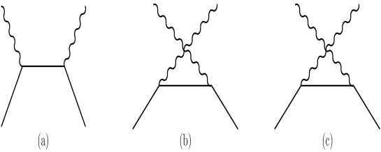
Figure 1: Diagrams relevant to Compton scattering.

One can now perform the (somewhat tedious) evaluation of the three lowest order Compton scattering diagrams shown in Figure 1, yielding the result

$${\rm Amp} = e^{2}\{2\epsilon_{A}\cdot\epsilon_{B}\left[{\epsilon_{1}\cdot p_{1}\epsilon_{2}\cdot p_{2}\over p_{1}\cdot k_{1}}-{\epsilon_{1}\cdot p_{2}\epsilon_{2}\cdot p_{1}\over p_{1}\cdot k_{2}}-\epsilon_{1}\cdot\epsilon_{2}\right]$$ (32)

$$- g\left[\epsilon_{A}\cdot[\epsilon_{2},k_{2}]\cdot\epsilon_{B}\left({\epsilon_{1}\cdot p_{1}\over p_{1}\cdot k_{1}}-{\epsilon_{1}\cdot p_{2}\over p_{1}\cdot k_{2}}\right)-\epsilon_{A}\cdot[\epsilon_{1},k_{1}]\cdot\epsilon_{B}\left({\epsilon_{2}\cdot p_{2}\over p_{1}\cdot k_{1}}-{\epsilon_{2}\cdot p_{1}\over p_{1}\cdot k_{2}}\right)\right]$$

$$- g^{2}\left[{1\over 2p_{1}\cdot k_{1}}\epsilon_{A}\cdot[\epsilon_{1},k_{1}]\cdot[\epsilon_{2},k_{2}]\cdot\epsilon_{B}-{1\over 2p_{1}\cdot k_{2}}\epsilon_{A}\cdot[\epsilon_{2},k_{2}]\cdot[\epsilon_{1},k_{1}]\epsilon_{B}\right]$$

$$- {(g-2)^{2}\over m^{2}}\left[{1\over 2p_{1}\cdot k_{1}}\epsilon_{A}\cdot[\epsilon_{1},k_{1}]\cdot p_{1}\epsilon_{B}\cdot[\epsilon_{2},k_{2}]\cdot p_{2}\right.$$

$$- \left.{1\over 2p_{1}\cdot k_{2}}\epsilon_{A}\cdot[\epsilon_{2},k_{2}]\cdot p_{1}\epsilon_{B}\cdot[\epsilon_{1},k_{1}]\cdot p_{1}\right]\}$$

where we have defined

$$S\cdot[Q,R]\cdot T\equiv S\cdot QT\cdot R-S\cdot RT\cdot Q.$$

The intriguing terms here are those on the last two lines, which are proportional to the factor $1/m^{2}$. They arise from the Born diagrams via the $k_{\alpha}k_{\beta}$ piece of the spin-one propagator

$$D_{\alpha\beta}(k)={i\over k^{2}-m^{2}}(-g_{\alpha\beta}+{k_{\alpha}k_{\beta}\over m^{2}})$$ (33)

and reveal that if we take the limit as the charge stays fixed and the mass becomes small the Compton amplitude will diverge, violating unitarity at a photon energy $\omega_{i}\sim m$ unless the gyromagnetic ratio has the value $g=2$! Remarkably, the condition $g=2$ has been demonstrated by Ferrara, Porrati, and Telegdi to assure the absence of $1/m^{2}$ terms for arbitrary spin[10], which is certainly suggestive that the “natural” value of the g-factor should be $g_{S}=2$.

3.2 The GDH Sum Rule

The Gerasimov, Drell, Hearn sum rule relates the anomalous magnetic moment of a system of spin $S$ to a weighted integral over polarized photon cross sections. It was originally derived for the nucleon and has the form

$${\alpha\kappa^{2}\over m^{2}}={1\over\pi^{2}}\int_{0}^{\infty}{d\omega\over\omega}(\sigma_{3\over 2}(\omega)-\sigma_{1\over 2}(\omega))$$ (34)

where here $\kappa$ is the anomalous magnetic moment, while $\sigma_{3\over 2}(\omega)$, $\sigma_{1\over 2}(\omega)$ are the laboratory frame scattering cross sections involving a polarized nucleon target and circularly polarized photons whose helicity is parallel, antiparallel to the target spin. It is derived simply by assuming analyticity of the Compton amplitude together with crossing symmetry and convergence and is a very fundamental sum rule about which much has been written[19]. Recent experimental studies have shown that it is satisfied in the case of a nucleon target[19].The GDH sum rule is also closely connected to the celebrated Bjorken sum rule[21]

$$\int_{0}^{1}(g_{1}^{\rm p}(x)-g_{1}^{\rm n}(x))={1\over 6}g_{A}$$ (35)

which relates the difference of polarized proton and neutron inclusive electron scattering structure functions to the axial decay constant of the neutron. For these reasons the GDH sum rule can be considered to be very fundamental and generally valid for arbitrary targets even though it has been experimentally verified only for the nucleon. The generalization of the GDH sum rule to the case of arbitrary spin $S$ has been given by Weinberg[20], who showed that it has the form

$${\alpha\over 4M^{2}}(g_{S}-2)^{2}={1\over\pi^{2}}\int_{0}^{\infty}{d\omega\over\omega}[\sigma_{1+S}(\omega)-\sigma_{1-S}(\omega)]$$ (36)

where here the cross sections are scattering cross sections circularly polarized photons with their polarization parallel and anti parallel to that of a maximally polarized target of spin $S$. If as in the nucleon case, we define what is measured here as the anomalous magnetic moment, then we see that this anomalous moment is defined in terms of the difference of the experimental g-factor from a bare value—$g_{\rm bare}=2$—again supporting the suggestion that the ”natural” value of the g-factor should be $g_{S}=2$, independent of spin.

3.3 Graviton Scattering and Factorization

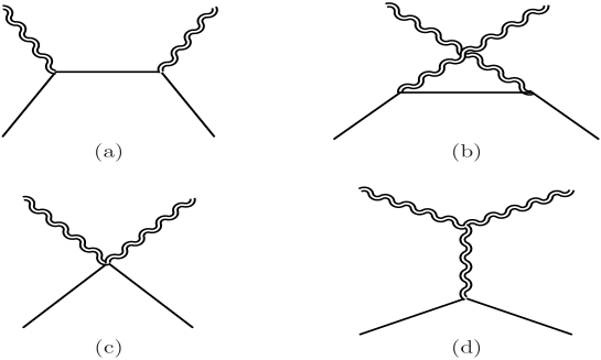
Figure 2: Diagrams relevant for gravitational Compton scattering.

Using powerful (string-based) techniques, which simplify conventional quantum field theory calculations, it has recently been demonstrated that the elastic scattering of gravitons from a target of arbitrary spin must factorize[22], a feature that had been noted ten years previously by Choi et al. based on gauge theory arguments[23]. That is, a (in harmonic gauge) graviton is a particle of spin 2 whose polarization vector $\epsilon_{\mu\nu}$ can be written as a simple product of the corresponding spin one photon polarization vectors—

$$\epsilon_{\mu\nu}^{\pm 2}=\epsilon_{\mu}^{\pm 1}\epsilon_{\nu}^{\pm 1}$$

The elastic scattering of gravitons from a target of arbitrary spin is constructed from the four diagrams shown in Figure 2, consisting of two Born diagrams, a seagull term, and the graviton pole diagram. The factorization theorem asserts that for scattering from a target of spin $S$, the graviton scattering amplitude can be written in the form

$$\epsilon_{f}^{*\alpha\beta}M^{G}_{\alpha\beta;\mu\nu}\epsilon_{i}^{\mu\nu}=F\times(\epsilon_{f}^{*\alpha}A^{C}_{\alpha;\mu}(S)\epsilon_{i}^{\mu})\times(\epsilon_{f}^{*\alpha}A^{C}_{\alpha;\mu}(0)\epsilon_{i}^{\mu})$$ (37)

where $M^{G}_{\alpha\beta;\mu\nu}$ is the elastic graviton scattering amplitude, $A^{C}_{\alpha\mu}(S)$ is the elastic Compton amplitude from a target of spin $S$, and F is the kinematic factor

$$F={G\over 4\pi\alpha^{2}}{p_{1}\cdot k_{1}p_{1}\cdot k_{2}\over k_{1}\cdot k_{2}}$$ (38)

with $\alpha=e^{2}/4\pi$ and $G$ being the fine structure and Newton constants respectively. The full graviton scattering amplitude could in principle have terms proportional to $1/m^{2}$ from the Born diagrams and the propagator of the spin-$S$ system. However, this does not occur. This can be seen in the case of a spin one system from the form of the half-off-shell energy-momentum tensor, which determines the gravitational coupling

$$<p_{2},\lambda|T_{\mu\nu}|p_{1},\epsilon_{A}> = \epsilon_{A\lambda}(p_{2\mu}p_{1\nu}+p_{1\nu}p_{2\mu})+g_{\mu\nu}p_{1\lambda}\epsilon_{A}\cdot p_{2}$$ (39)

$$- p_{1\lambda}(p_{2\mu}\epsilon_{A\nu}+p_{2\nu}\epsilon_{A\mu})-\epsilon_{A}\cdot p_{2}(p_{1\mu}g_{\lambda\nu}+p_{1\nu}g_{\lambda\mu})$$

$$+ (p_{2}\cdot p_{1}-m^{2})(g_{\lambda\mu}\epsilon_{A\nu}+\epsilon_{A\mu}g_{\lambda\nu}-g_{\mu\nu}\epsilon_{A\lambda})$$

Taking $p_{1}$ to be physical—$p_{1}^{2}=m^{2}$—but $p_{2}$ to be an off-shell intermediate state momentum, we find that when $T_{\mu\nu}$ is contracted with the $1/m^{2}$ piece of the spin one propagator—${p_{2}^{\alpha}p_{2}^{\lambda}\over m^{2}}$—the result is independent of $m^{2}$—

$${p_{2}^{\alpha}p_{2}^{\lambda}\over m^{2}}<p_{2},\lambda|T_{\mu\nu}|p_{1},\epsilon_{A}>=p_{2}^{\alpha}(g_{\mu\nu}\epsilon_{A}\cdot p_{2}-\epsilon_{A\mu}p_{2\nu}-\epsilon_{A\nu}p_{2\mu})$$ (40)

The coefficient $1/m^{2}$ in the spin one propagator has cancelled. Thus no term proportional to $1/m^{2}$ survives in the Born amplitude and this vanishing of terms which diverge as $m\rightarrow 0$ can be shown to be a general property regardless of the spin of the target. According to the factorization condition, the vanishing of $1/m^{2}$ terms in the gravitational amplitude can only result from the vanishing of such terms in the corresponding Compton amplitude, which we have already seen occurs only if the value $g_{S}=2$ is chosen, so from an additional standpoint we see that the “natural” value for the g-factor is $g=2$.

4 Conclusions

Above we have examined the question of whether there exists a “natural” value for the gyromagnetic ratio of a fundamental particle of spin $S$. One might think that this question was answered long ago when Belinfante conjectured and others proved the assertion that when minimal substitution is used in order to generate the electromagnetic interactions os a system of spin $S$, the resulting g-factor is given by $g=1/S.$ However, while this prediction is consistent with the case of the electron, we showed that in the standard model of electroweak interactions the only other example of a charged fundamental particle—the $W^{\pm}$ boson—does not agree with this prediction. Rather, due to gauge invariance, the result $g_{W}=2$ is found. We then went on to argue that, while there are no additional experimental cases, the “natural” value $g=2$ for all systems is supported by at least three theoretical arguments:

• Use of $g_{S}=2$ guarantees the vanishing of terms proportional to $1/m^{2}$ in the Compton scattering amplitude from a system of spin $S$, whose presence would violate unitarity at the very low energy scale $\omega\sim m$.

• The fundamental GDH sum rule allows experimental measurement of the anomalous magnetic moment for a system of arbitrary spin $S$, where the anomalous moment is

  $$\kappa=g_{\rm exp}-g_{S}$$

  with $g_{S}=2$ being the ”natural” value of the g-factor.

• Based on the result that the graviton scattering amplitude from a system of spin-S must factorize into a product of Compton amplitudes, the vanishing of $1/m^{2}$ terms in the graviton amplitude is found to result from the choice $g_{S}=2$ in the corresponding Compton amplitude.

Although for simplicity we shall not discuss them here there exist even more reasons for this assertion[10],[11].

• The only known example of a completely consistent theory of interacting particles of spin greater than two is string theory, and for open strings it is possible to obtain the exact equations of motion for massive charged particles of arbitrary spin, moving in a constant, external electromagnetic background. This procedure yields $g_{S}=2$ for all spins[24].

• The classical relativistic equation of motion of the polarization vector $S_{\mu}$ in a homogeneous external electromagnetic field is given by the Bargmann, Michel, Telegdi or BMT equation[25]

  $${dS^{\mu}\over d\tau}={eg\over 2m}F^{\mu\nu}S_{\nu}+{e\over 2m}(g-2){dx^{\mu}\over d\tau}F^{\nu\lambda}S_{\nu}{dx_{\lambda}\over d\tau}$$ (41)

  which simplifies for $g_{S}=2$ independent of the spin of the particle.

• In general relativity the $G\rightarrow 0$ limit of the Kerr-Newman metric describing spacetime around a charged spinning mass results in an electromagnetic field in flat space with $g=2$. Additional arguments from general relativity can be found in [11].

For these and other reasons then, it appears that the “natural” value for the g-factor is $g_{S}=2$ regardless of spin. Since there are no experimental manifestations of this result outside of the electron and $W^{\pm}$-boson systems, this discussion could be argued to be somewhat metaphysical, but the totality of the arguments given above together with the standard model value of the $W^{\pm}$ moment would seem to constitute a rather compelling case.

Acknowledgements

This work was supported in part by the National Science Foundation under award PHY 02-44801. Thanks to Prof. A. Faessler and the theoretical physics group at the University of Tübingen, where this work was completed, for hospitality.

5 Appendix: Nonrelativisitic Reduction

As an alternative derivation of Belinfante’s result, it is useful to understand how to construct an effective nonrelativistic Schrödinger Hamiltonian from a given relativistic Lagrangian[12]. In this way, for example, one finds the familiar Dirac prediction that for a fundamental spin 1/2 system we have $g=2$.

5.1 Spin 1/2

In order to see how this prediction comes about, we begin with the Dirac equation in the absence of electromagnetism

$$(i\not\!{\nabla}-m)\psi(x)=0$$ (42)

where $\not\!{V}$ implies contraction of the four-vector $V_{\mu}$ with the Dirac matrices—$\gamma_{0}V_{0}-\vec{\gamma}\cdot\vec{V}$. Now assume that we can account for coupling to electromagnetism via the minimal substitution

$$i\nabla_{\mu}\longrightarrow\pi_{\mu}\equiv i\nabla_{\mu}-eA_{\mu}$$ (43)

so that the Dirac equation becomes

$$(\not\!{\pi}-m)\psi(x)=0$$ (44)

Using the conventional representation for the Dirac matrices[8]

$$\gamma_{0}=\left(\begin{array}[]{cc}1&0\\ 0&1\end{array}\right),\quad\vec{\gamma}=\left(\begin{array}[]{cc}0&\vec{\sigma}\\ -\vec{\sigma}&0\end{array}\right)$$ (45)

we can write the Dirac equation as a set of two coupled equations relating the upper ($\psi_{a}$) and lower ($\psi_{b}$) components of the wavefunction. That is, for a positive energy solution

$$\psi(\vec{x},t)=\left(\begin{array}[]{c}\psi_{a}(\vec{x})\\ \psi_{b}(\vec{x})\end{array}\right)\exp(-i(m+W)t)$$ (46)

we have

$$(m+W-e\varphi)\psi_{a}-\vec{\sigma}\cdot\vec{\pi}\psi_{b} = m\psi_{a}$$

$$\vec{\sigma}\cdot\vec{\pi}\psi_{a}-(m+W-e\varphi)\psi_{b} = m\psi_{b}$$ (47)

Solving the second of these for the lower component we find

$$\psi_{b}={1\over 2m+W-e\varphi}\vec{\sigma}\cdot\vec{\pi}\psi_{a}$$ (48)

and substitution into the first yields

$$\vec{\sigma}\cdot\vec{\pi}{1\over 2m+W-e\varphi}\vec{\sigma}\cdot\vec{\pi}\psi_{a}=(W-e\varphi)\psi_{a}$$ (49)

which in the nonrelativistic limit—$W<<m$—becomes

$$\left[{1\over 2m}\vec{\sigma}\cdot\vec{\pi}\vec{\sigma}\cdot\vec{\pi}+e\varphi\right]\psi_{a}=W\psi_{a}$$ (50)

and produces the effective Schrödinger Hamiltonian

$$H_{\rm eff}={1\over 2m}\vec{\sigma}\cdot\vec{\pi}\vec{\sigma}\cdot\vec{\pi}+e\varphi$$ (51)

Using the Pauli matrix identity

$$\sigma_{a}\sigma_{b}=\delta_{ab}+i\epsilon_{abc}\sigma_{c}$$ (52)

this becomes the expected result

$$H_{\rm eff}={(\vec{p}^{2}-e\vec{A})^{2}\over 2m}-{e\over 2m}\vec{\sigma}\cdot\vec{B}+e\phi$$ (53)

and comparison with the definition Eq. 1 and the usual expression for the interaction energy of a magnetic dipole

$$U=-\vec{\mu}\cdot\vec{B}$$ (54)

yields the prediction $g=2$.

5.2 Spin Zero

In order to see how to handle the case of unit spin, it is useful to first review the method to obtain the effective Schrödinger equation for the case of spin zero. We begin with the Klein-Gordon equation

$$(\Box+m^{2})\phi=0$$ (55)

and include electromagnetism via the minimal substitution, so that Eq. 55 assumes the form

$$(\pi^{2}-m^{2})\phi=0$$ (56)

A problem here is that this equation is second order in time. Thus instead write it as a pair of coupled first order equations—

$$m\chi_{\mu} = \pi_{\mu}\phi$$

$$\pi^{\mu}\chi_{\mu} = m\phi$$ (57)

Note then that the vector components $\chi_{i}$ have no time development and can therefore be considered as a constraint—

$$\chi_{i}={1\over m}\pi_{i}\phi$$ (58)

We have then the two coupled equations

$$i{\partial\over\partial t}\chi_{0} = (m+e\varphi)\phi+{\vec{\pi}^{2}\over m}\phi$$

$$i{\partial\over\partial t}\phi = (m+e\varphi)\chi_{0}$$ (59)

Now write the equation in terms of a two component ”spinor”

$$\rho=\left(\begin{array}[]{c}\rho_{a}\\ \rho_{b}\end{array}\right)={1\over 2}\left(\begin{array}[]{c}\phi+\chi_{0}\\ \phi-\chi_{0}\end{array}\right)$$ (60)

We have then the equation

$$i{\partial\over\partial t}\rho=\left[m\tau_{3}+e\varphi+{\vec{\pi}^{2}\over 2m}(\tau_{3}+i\tau_{2})\right]\rho$$ (61)

Projecting out the positive energy solution via

$$\rho(\vec{x},t)=\rho(\vec{x})\exp(-i(m+W)t)$$

the lower component of the spinor equation then has the form

$$(m+W-e\varphi)\rho_{b}=-m\rho_{b}-{\vec{\pi}^{2}\over 2m}(\rho_{a}+\rho_{b})$$ (62)

and can be solved in the nonrelativistic limit to yield

$$\rho_{b}\simeq-{\vec{\pi}^{2}\over 4m^{2}}\rho_{a}$$ (63)

Substitution into the top component of the spinor equation then yields

$$W\rho_{a}\simeq[e\varphi+{\vec{\pi}^{2}\over 2m}-{\vec{\pi}^{4}\over 8m^{3}}]\rho_{a}$$ (64)

We have then the effective Schrödinger Hamiltonian

$$H_{\rm eff}=e\varphi+{(\vec{p}-e\vec{A})^{2}\over 2m}-{(\vec{p}-e\vec{A})^{4}\over 8m^{3}}+\ldots$$ (65)

as expected. Similar methods can be used in order to to treat the more challenging unit spin problem, as we now demonstrate.

5.3 Spin One

In the case of spin 1 the free particle equation of motion is given by the Proca equation[14],

$$\nabla^{\mu}U_{\mu\nu}+m^{2}U_{\nu}=(\Box+m^{2})U_{\nu}-\nabla_{\nu}\nabla\cdot U=0$$ (66)

where $U_{\mu\nu}$ is the field tensor

$$U_{\mu\nu}=\nabla_{\mu}U_{\nu}-\nabla_{\nu}U_{\mu}$$

Of course, a spin one field should only have three degrees of freedom, while the four-vector $U_{\mu}$ has four. However, from Eq. 66, we find, taking the divergence, that

$$m^{2}\nabla\cdot U=0$$ (67)

which, for non-massless particles, yields the desired constraint $\nabla\cdot U=0$. In order to include interactions with the electromagnetic field we make the minimal substitution—$i\nabla_{\mu}\rightarrow\pi_{\mu}$ as before, yielding the equation of motion

$$\pi^{\mu}(\pi_{\mu}U_{\nu}-\pi_{\nu}U_{\mu})-m^{2}U_{\nu}=0$$ (68)

and the constraint equation

$${1\over 2}[\pi^{\nu},\pi^{\mu}]U_{\mu\nu}=-i{e\over 2}F^{\mu\nu}U_{\mu\nu}=m^{2}\nabla\cdot U$$ (69)

In order to reduce this equation to a nonrelativistic form we need to rewrite it in terms of a pair of coupled first order equations[15]

$$\pi^{\mu}U_{\mu\nu}-m^{2}U_{\nu}=0$$

$$U_{\mu\nu}=\pi_{\mu}U_{\nu}-\pi_{\nu}U_{\mu}$$ (70)

We note then that the degrees of freedom $U_{0}$ and $U_{ij}$ do not contribute to the time development and can be considered as constraints

$$U_{ij}=\pi_{i}U_{j}-\pi_{j}U_{i}$$

$$U_{0}=-{1\over m^{2}}\vec{\pi}\cdot\vec{\phi}$$ (71)

where we have defined $U_{i0}=m\phi_{i}$. We find then the dynamical equations

$$i{\partial\over\partial t}\vec{\phi} = e\varphi\vec{\phi}+m\vec{U}-{1\over m}\vec{\pi}\times(\vec{\pi}\times\vec{U})$$

$$i{\partial\over\partial t}\vec{U} = e\varphi\vec{U}+m\vec{\phi}+{1\over m}\vec{\pi}\vec{\pi}\cdot\vec{\phi}$$ (72)

Defining the spin vectors

$$S_{x}=\left(\begin{array}[]{ccc}0&0&0\\ 0&0&-i\\ 0&i&0\end{array}\right),\quad S_{y}=\left(\begin{array}[]{ccc}0&0&i\\ 0&0&0\\ -i&0&0\end{array}\right),\quad S_{z}=\left(\begin{array}[]{ccc}0&-i&0\\ i&0&0\\ 0&0&0\end{array}\right)$$ (73)

and representing the vector quantities $\vec{\phi},\vec{U}$ in terms of three-component column vectors $\phi,U$, these equations become

$$i{\partial\over\partial t}\phi = e\varphi\phi+mU+{1\over m}(\vec{S}\cdot\vec{\pi})^{2}U$$

$$i{\partial\over\partial t}U = e\varphi U+m\phi-{1\over m}(\vec{S}\cdot\vec{\pi})^{2}\phi+{\vec{\pi}^{2}\over m}\phi-{e\over m}(\vec{S}\cdot\vec{B})\phi$$ (74)

As in the Klein-Gordon case we can write this as a six-component spinor equation by defining

$$\rho=\left(\begin{array}[]{c}\rho_{a}\\ \rho_{b}\end{array}\right)={1\over 2}\left(\begin{array}[]{c}\phi+U\\ \phi-U\end{array}\right)$$ (75)

so that the equation reads

$$i{\partial\over\partial t}\rho=[e\varphi+\tau_{3}m-i\tau_{2}{1\over m}(\vec{S}\cdot\vec{\pi})^{2}+(\tau_{3}+i\tau_{2}){1\over 2m}(\vec{\pi}^{2}+e\vec{S}\cdot\vec{B})]\rho$$ (76)

Projecting out the positive energy solution via

$$\rho(\vec{x},t)=\rho(\vec{x})\exp(-i(m+W)t)$$ (77)

we can solve for the lower component in the nonrelativistic limit, yielding

$$\rho_{b}\simeq-{1\over 2m}({\vec{\pi}^{2}\over 2m}-{e\over 2m}(\vec{S}\cdot\vec{B})-{1\over m}(\vec{S}\cdot\vec{\pi})^{2})\rho_{a}$$ (78)

and substitution into the top component yields the equation

$$W\rho_{a}=\left[e\varphi+{\vec{\pi}^{2}\over 2m}-{e\over 2m}(\vec{S}\cdot\vec{B})-{1\over 2m}({\vec{\pi}^{2}\over 2m}-{1\over m}(\vec{S}\cdot\vec{\pi})^{2})^{2}\right]\rho_{a}$$ (79)

We thus find the effective spin one Hamiltonian to be

$$H_{\rm eff}={(\vec{p}-e\vec{A})^{2}\over 2m}-{e\over 2m}\vec{S}\cdot\vec{B}-{(\vec{p}-e\vec{A})^{4}\over 8m^{3}}+\ldots$$ (80)

so that minimal substitution has yielded a value for the magnetic moment—$g=1=1/s$—which agrees with the Belinfante conjecture.

References

- [1] See, e.g., J.F. Donoghue, E. Golowich, and B.R. Holstein, Dynamics of the Standard Model, Cambridge Univ. Press, New York (1992), Ch. V-1.
- [2] R.P. Feynman, Quantum Electrodynamics, Benjamin, New York (1961).
- [3] H.A. Bethe and F. deHoffman, Mesons and Fields, MIT Press, Cambridge, MA (1970), Vol. 2.
- [4] F.J. Belinfante, “Intrinsic Magnetic Moment of Elementary Particles of Spin 3/2,” Phys. Rev. 92, 997-1001 (1953).
- [5] P.A. Moldauer and K.M. Case, “Properties of Half-Integral Spin Dirac-Fierz-Pauli Particles,” Phys. Rev. 102, 279-85 (1956); K.M. Case, “Hamiltonian Form of Integral Spin Wave Equations,” Phys. Rev. 100, 1513-14 (1955); R.F. Guertin, “Foldy-Wouthuysen Transformations for Any Spin,” Ann. Phys. (NY), 386-412 (1975); R. Cecchini and M. Tarlini, “Arbitrary-Spin Particles in an Electromagnetic Field,” Nuovo Cim. A47, 1-11 (1978).
- [6] C.R. Hagen and W.J. Hurley, ”Magnetic Moment of a Particle with Arbitrary Spin,” Phys. Rev. Lett. 24, 1381 (1970).
-
[7]
J.D. Jackson, Classical Electrodynamics, wiley,
New York (1970) shows that in the presence of interactions with an
external vector potential the relativistic
Hamiltonian in the absence of
is replaced by
Making the quantum mechanical substituations
we find the minimal substitution given in the text. - [8] See, e.g., J.D. Bjorken and S.D. Drell, Relativistic Quantum Mechanics, McGraw-Hill, New York (1964).
- [9] I.J.R. Aitchison and A.J.G. Hey, Gauge Theories in Particle Physics, Adam Hilger, Philadelphia (1989) Ch. 8.
- [10] S. Ferrara, M. Porrati, and V.L. Telegdi, “g=2 as the Natural Value of the Tree-Level Gyromagnetic Ratio of Elementary Particles,” Phys. Rev. D46, 3529-37 (1992).
- [11] H. Pfister and M. King, ”The Gyromagnetic Factor in electrodymamics, Quantum Theory and General Relativity,” Class. Quant. Gravity 20, 205-13 (2003).
- [12] B.R. Holstein, “Diagonalization of the Dirac Equation: an Alternate Approach,” Am. J. Phys. 65, 519-22 (1997).
- [13] An interesting historical footnote, as noted by Drechsel, is that when Stern originally proposed measurement of a possible deviation of the proton moment from the Dirac prediction, Pauli assured him that this was a waste of time. It is thus ironic that this anomalous magnetic moment piece is called the Pauli term.
- [14] A. Proca, “Sur les Equations Fondamentales des Particules Elementaires,” Comp. Ren. Acad. Sci. Paris 202, 1366 (1936).
- [15] J.A. Young and S.A. Bludman, “Electromagnetic Properties of a Charged Vector Meson,” Phys. Rev. 131, 2326-34 (1963).
- [16] Particle Data Group, S. Eidelman et al., Phys. Lett. B592, 1 (2004).
-
[17]
One can see this result by using the
representations of the rest frame polarization vectors of the spin
1 bosons quantized along the -direction
and verifying, for example that
Similarly the other matrix elements can be checked. - [18] See, e.g., B.R. Holstein, Weak Interactions in Nuclei, Princeton Univ. Press, Princeton (1988), Ch. 3.
- [19] D. Drechsel and L. Tiator, ”The Gerasimov-Drell-Hearn Sum Rule and the Spin structure of the Nucleon,” Ann.Rev. Nucl. Part. Science 54, 69-114 (2004).
- [20] S. Weinberg, in Lectures on Elementary Paricles and Quantum Field Theory, Proc. Summer Institute, Brandeis Univ. (1970), ed. S. Deser, MIT Press, Cambridge, MA (1970), Vol. 1.
- [21] J.D. Bjorken, “Applications of the U(6)U(6) Algebra of Current Densities,” Phys. Rev. 148, 1467-78 (1966); “Inelastic Scattering of Polarized Leptons from Polarized Nucleons,” Phys. Rev. D1, 1376-79 (1970).
- [22] Z. Bern, “Perturbative Quantum Gravity and its Relation to Gauge Theory,” [archiv:gr-qc/0206071].
- [23] S.Y. Choi, J.S. Shim, and H.S. Song, “Factorization and Polarization in Linearized Gravity,” Phys. Rev. D51, 2751-69 (1995).
- [24] P.C. Argyres and C.R. Nappi, “Massive Spin-2 Bosonic String States in an Electromagentic Background,” Phys. Lett. B244, 89-96 (1989).
- [25] V. Bargmann, L. Michel, and V.L. Telegdi, “Precession of the Polarization of Particles Moving in a Homogeneous Electromagnetic Field,” Phys. Rev. Lett. 2, 435-36 (1959).