The high-energy limit of inclusive and diffractive deep inelastic scattering in QCD

Abstract

Following recent progresses in the understanding of high-energy scattering in QCD, we derive the first phenomenological consequences of Pomeron loops, in the context of both inclusive and diffractive deep inelastic scattering. In particular, we discuss diffusive scaling, a new scaling law that emerges for sufficiently high energies and up to very large values of $Q^{2},$ well above the proton saturation momentum.

1 Introduction

The Good-and-Walker picture of diffraction was originally meant to describe soft diffraction. They express an hadronic projectile $|P\rangle\!=\!\sum_{n}c_{n}|e_{n}\rangle$ in terms of hypothetic eigenstates of the interaction with the target $|e_{n}\rangle,$ that can only scatter elastically: $\hat{S}|e_{n}\rangle\!=\!(1\!-\!T_{n})|e_{n}\rangle.$ The total, elastic and diffractive cross-sections are then easily obtained:

$$\sigma_{tot}=2\sum_{n}c_{n}^{2}T_{n}\hskip 14.22636pt\sigma_{el}=\Big{[}\sum_{n}c_{n}^{2}T_{n}\Big{]}^{2}\hskip 14.22636pt\sigma_{diff}=\sum_{n}c_{n}^{2}T_{n}^{2}\ .$$ (1)

It turns out that in the high energy limit, there exists a basis of eigenstates of the large$-N_{c}$ QCD $S-$matrix: sets of quark-antiquark dipoles $|e_{n}\rangle\!=\!|d(r_{1}),\dots,d(r_{n})\rangle$ caracterized by their transverse sizes $r_{i}.$ In the context of deep inelastic scattering (DIS), we also know the coefficients $c_{n}$ to express the virtual photon in the dipole basis. For instance, the equivalent of $c_{1}^{2}$ for the one-dipole state is the photon wavefunction $\phi(r,Q^{2}).$

This realization of the Good-and-Walker picture allows to write down an exact (within the high-energy and large$-N_{c}$ limits) factorization formula [1] for the diffractive cross-section in DIS in terms of dipole scattering amplitudes off the target proton, such as $\left\langle T(r_{1})\dots T(r_{n})\right\rangle_{Y}.$ The average $\langle\ .\ \rangle_{Y}$ is an average over the proton wavefunction which gives the energy dependence to the cross-section ($Y\!=\!\log(1/x)\!\sim\!\log(s)$ is the rapidity).

2 The geometric and diffusive scaling regimes

Within the high-energy and large$-N_{c}$ limits, the dipole amplitudes are obtained from the Pomeron-loop equation [2] derived in the leading logarithmic approximation in QCD. This is a Langevin equation which exhibits the stochastic nature [3] of high-energy scattering processes in QCD. Its solution is an event-by-event dipole scattering amplitude function of $\rho\!=\!-\log(r^{2}Q_{0}^{2})$ and $Y$ ($Q_{0}$ is a scale provided by the initial condition). It is characterized by a saturation scale $Q_{s}$ which is a random variable whose logarithm is distributed according to a Gaussian probability law [4]. The average value is $\log(\bar{Q}_{s}^{2}/Q_{0}^{2})\!=\!\lambda Y$ and the variance is $\sigma^{2}\!=\!DY$ (see Fig.1). The dispersion coefficient $D$ allows to distinguish between two energy regimes: the geometric scaling regime ($DY\!\ll\!1$) and diffusive scaling regime ($DY\!\gg\!1$).

The following results for the averaged amplitude will be needed to derive the implications for inclusive and diffractive DIS:

$$\left\langle T(r_{1})\dots T(r_{n})\right\rangle_{Y} \stackrel{{\scriptstyle Y\ll 1/D}}{{=}} \left\langle T(r_{1})\right\rangle_{Y}\dots\left\langle T(r_{n})\right\rangle_{Y}\ ,$$ (2)

$$\left\langle T(r_{1})\dots T(r_{n})\right\rangle_{Y} \stackrel{{\scriptstyle Y\gg 1/D}}{{=}} \left\langle T(r_{<})\right\rangle_{Y},\hskip 8.5359ptr_{<}=\min(r_{1},\dots,r_{n})\ .$$ (3)

All the scattering amplitudes are expressed in terms of $\langle T(r)\rangle_{Y},$ the amplitude for a single dipole which features the following scaling behaviors:

$$\left\langle T(r)\right\rangle_{Y}\stackrel{{\scriptstyle Y\ll 1/D}}{{\equiv}}T_{gs}(r,Y) = \displaystyle T\left(r^{2}\bar{Q}_{s}^{2}(Y)\right)\ ,$$ (4)

$$\left\langle T(r)\right\rangle_{Y}\stackrel{{\scriptstyle Y\gg 1/D}}{{\equiv}}T_{ds}(r,Y) = \displaystyle T\left(\frac{\log(r^{2}\bar{Q}_{s}^{2}(Y))}{\sqrt{DY}}\right)\ .$$ (5)

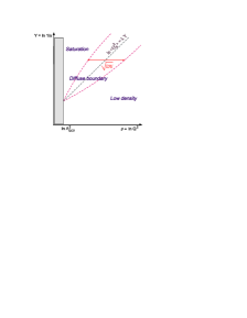
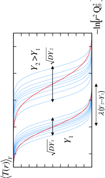
Figure 1: Left plot: a diagram representing the stochastic saturation line in the $(\rho,Y)$ plane, the diffusive saturation boundary is generated by the evolution. Right plot: different realizations of the event-by-event scattering amplitude (gray curves) and the resulting averaged physical amplitude $\langle T(r)\rangle$ (black curve) as a function of $\rho$ for two different values of $Y$ in the diffusive scaling regime.

3 Implications for inclusive and diffractive DIS

We shall concentrate on the diffusive scaling regime, in which the dipole scattering amplitude can be written as follows [5] for $-\log(r^{2}\bar{Q}_{s}^{2}(Y))\!\ll\!DY:$

$$T_{ds}(r,Y)=\frac{1}{2}Erfc\left(-\frac{\log(r^{2}\bar{Q}_{s}^{2}(Y))}{\sqrt{DY}}\right)\ .$$ (6)

From this, one obtains the following analytic estimates [1] for the $\gamma^{*}\!-\!p$ total cross-section in DIS and for the diffractive one integrated over $\beta$ from $\beta_{<}:$

$$\frac{d\sigma_{tot}}{d^{2}b}(x,Q^{2}) = \frac{N_{c}\alpha_{em}}{12\pi^{2}}\sum_{f}e_{f}^{2}\sqrt{\pi D\log(1/x)}\ \frac{e^{-Z^{2}}}{Z^{2}}\ ,$$ (7)

$$\frac{d\sigma_{diff}}{d^{2}b}(x,Q^{2},\beta_{<}) = \frac{N_{c}\alpha_{em}}{48\pi^{2}}\sum_{f}e_{f}^{2}\sqrt{D\log(1/x)}\ \frac{e^{-2Z^{2}}}{Z^{3}}\ .$$ (8)

The variable $Z$ is reminiscent of the scaling variable of the dipole amplitude:

$$Z=\frac{\log(Q^{2}/\bar{Q}_{s}^{2}(x))}{\sqrt{D\log(1/x)}}$$ (9)

and shows that in the diffusive scaling regime, both inclusive and diffractive scattering are dominated by small dipole sizes $r\!\sim\!1/Q.$ Also the cross-sections do not feature any Pomeron-like (power-law type) increase with the energy and the diffractive cross-section (which does not depend on $\beta_{<}$) is dominated by the scattering of the quark-antiquark ($q\bar{q}$) component, corresponding to $\beta\lesssim 1.$ These features a priori expected in the saturation regime ($Q^{2}<\bar{Q}_{s}^{2}$) are valid up to values of $Q^{2}$ much bigger than $\bar{Q}_{s}^{2}:$ in the whole diffusive scaling regime for $\log(Q^{2}/\bar{Q}_{s}^{2}(Y))\!\ll\!DY$ (see Fig.2).

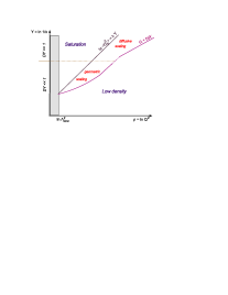
Figure 2: A phase diagram for the high-energy limit of inclusive and diffractive DIS in QCD. Shown are the average saturation line and the approximate boundaries of the scaling regions at large values of $\rho\!\sim\!\ln Q^{2}.$ With increasing $Y,$ there is a gradual transition from geometric scaling at intermediate energies to diffusive scaling at very high energies.

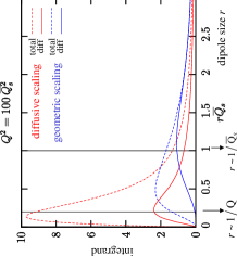
Figure 3: The integrands of (10) plotted as a function of $r\bar{Q}_{s}$ and computed with two expressions for the dipole amplitude: in the geometric and diffusive scaling regimes.

The inclusive cross-section and the $q\bar{q}$ contribution to the diffractive one are obtained from the dipole amplitude $\langle T(r)\rangle_{Y}$ in the following way:

$$\frac{d\sigma_{tot}}{2\pi\ d^{2}b}=\int dr^{2}\Phi(r,Q^{2})\langle T(r)\rangle_{Y}\ ,\,\frac{d\sigma_{diff}}{\pi\ d^{2}b}=\int dr^{2}\Phi(r,Q^{2})\langle T(r)\rangle^{2}_{Y}\ .$$ (10)

In order to better exhibit the dominance of small dipole sizes $r\!\sim\!1/Q$, we represent in Fig.3 the integrands of (10) as a function of the dipole size $r.$ Keeping $Q/\bar{Q}_{s}\!=\!10$ fixed, we use (6) in the diffusive scaling regime and $T_{gs}(r,Y)\!=\!1\!-\!e^{-r^{2}\bar{Q}_{s}^{2}(Y)/4}$ in the geometric scaling regime. The difference between the geometric and diffusive scaling is striking. For the latter, both inclusive and diffractive scattering are dominated by inverse dipole sizes of the order of the hardest infrared cutoff in the problem: the hardest fluctuation of the saturation scale, which is as large as $Q.$

In the diffusive scaling regime, up to values of $Q^{2}$ much bigger than the saturation scale $\bar{Q}_{s}^{2}$, cross-sections are dominated by rare events in which the photon hits a black spot that he sees at saturation at the scale $Q^{2}.$ In average the scattering is weak, but saturation is the only relevant physics.

References

• [1] Y. Hatta, E. Iancu, C. Marquet, G. Soyez and D. Triantafyllopoulos, Nucl. Phys. A773 (2006) 95; E. Iancu, C. Marquet and G. Soyez, hep-ph/0605174.
• [2] A.H. Mueller, A.I. Shoshi and S.M.H. Wong, Nucl. Phys. B715 (2005) 440;
E. Iancu and D.N. Triantafyllopoulos, Phys. Lett. B610 (2005) 253.
• [3] A.H. Mueller and A.I. Shoshi, Nucl. Phys. B692 (2004) 175;
E. Iancu, A.H. Mueller and S. Munier, Phys. Lett. B606 (2005) 342.
• [4] E. Brunet, B. Derrida, A.H. Mueller and S. Munier, cond-mat/0512021;
C. Marquet, G. Soyez and B.-W. Xiao, hep-ph/0606233.
• [5] E. Iancu and D.N. Triantafyllopoulos, Nucl. Phys. A756 (2005) 419;
C. Marquet, R. Peschanski and G. Soyez, Phys. Rev. D73 (2006) 114005.