Probing Dark Energy via Neutrino & Supernova Observatories

Abstract

A novel method for extracting cosmological evolution parameters is proposed, using a probe other than light: future observations of the diffuse anti-neutrino flux emitted from core-collapse supernovae (SNe), combined with the SN rate extracted from future SN surveys. The relic SN neutrino differential flux can be extracted by using future neutrino detectors such as Gadolinium-enriched, megaton, water detectors or 100-kiloton detectors of liquid Argon or liquid scintillator. The core-collapse SN rate can be reconstructed from direct observation of SN explosions using future precision observatories. Our method, by itself, cannot compete with the accuracy of the optical-based measurements but may serve as an important consistency check as well as a source of complementary information. The proposal does not require construction of a dedicated experiment, but rather relies on future experiments proposed for other purposes.

I Introduction

The acceleration of the rate of expansion of the Universe, first discovered through the dimming of distant Type Ia supernovae Perlmutter:1998np ; Riess:1998cb , is being confirmed by various new cosmological tests. The cosmic microwave background measurements by the Wilkinson Microwave Anisotropic Probe (WMAP) Spergel:2003cb and the results from the large scale distribution of galaxies Percival:2001hw ; Eisenstein:2005su and galaxy clusters Allen:2002eu confirm that our universe is dominated by a fluid of negative pressure. The understanding of the accelerated expansion of the cosmos might result in a change of our description of gravity or in the identification of unknown components of the cosmos. Since this is of utmost importance to fundamental physics, large sets of cosmological data and various procedures to analyze them are being examined.

The correct identification of what composes the fluid of negative pressure or “Dark Energy” is one of the most challenging issues at the interface between particle physics and modern cosmology. Detecting the acceleration with a probe that interacts differently from photons can provide a new insight into this puzzling issue. The only particles at our disposal that can be used for such a task are the diffuse supernova (SN) neutrinos emitted from core collapse (CC) SNe. As discussed in more detail below, most of the massive stars in our universe (with mass above about 5-8 solar masses) end their lives with a violent collapse. During this collapse the massive stars release a huge flux of neutrinos. Thus a continuous and isotropic flux of neutrinos from very far CC SNe is expected to be present. It is commonly denoted as the diffuse SN neutrino flux or supernova relic neutrino (SRN) flux.

In this paper we investigate the possibility that information on the parameters governing the accelerated expansion may be extracted by using measurements that do not solely rely on detection of luminous objects and the knowledge of their intensity. We propose that the observation of the SRN, when combined with improved measurements of the past supernova explosion rate, may provide an independent source of information on the cosmological evolution parameters.

Future megaton (Mt) water-Cherenkov detectors (such as UNO UNO , Hyper-Kamiokande HyperK or MEMPHYS MEMPHYS ), if enriched by Gadolinium-rich material (see the GADZOOKS! proposal GAD ), are capable of observing hundreds of supernova relic neutrinos (SRNs) per year. In addition we expect a significant improvement in the amount of data that will be available from the direct detection of CC SN explosions with future SN surveys like DESTINY Destiny , DUNE DUNE , JEDI JEDI , LSST LSST or SNAP SNAP . This will yield a direct measurement of the SN CC rate as a function of redshift, $R_{\rm SN}(z)$, as opposed to an indirect estimate based on the cosmic star formation history (SFH), which is subject to sizable uncertainties.

Our basic idea can be described as replacing the photons from Type Ia SNe, standard(izable) light candles, with neutrinos emitted from CC SNe. The latter may roughly be viewed as “standard neutrino candles”. Unlike the case of photons from Type Ia SN, the detection of SRNs cannot be correlated with individual CC events. Only the integrated energy spectrum of neutrinos emitted from SNe at various distances and directions will be available. Thus, this signal by itself cannot be used in order to extract information on cosmology since it measures an “averaged” flux of SN neutrinos coming from sources at various distances. However, when combined with a future measurement of the CC SNe explosion rate, the neutrino signal does carry valuable cosmological information.

Let us schematically describe the basic elements of our method:

• Future neutrino experiments will provide us with rather accurate information on the SRN differential flux $dF/dE$.

• Future direct observation of supernovae at different redshifts will provide us with an estimate for the CC supernova rate, $R_{\rm SN}^{\rm obs}(z)$.

• The above observables both depend on the comoving CC supernova rate $R_{\rm SN}(z)$, but with a different dependence on cosmology. Thus we can combine the above measurements to extract data on the cosmological evolution parameters.

• The dependence on the star formation rate, known only to a rough accuracy, cancels when combining the two measurements. This large source of uncertainty drops out of our extraction of cosmological evolution parameters.

Without understanding the related systematic uncertainties, however, extraction of useful information from such measurements is impossible. At this stage, with the present theoretical and experimental knowledge, it is not completely clear whether the above is a realistic task. Below we present several aspects of our study in more details, in particular we describe how our proposal could work in practice for an optimal case study. Next we discuss the various uncertainties involved, pointing out several directions that may help in decreasing them. To show how our proposal works, as a matter of principle, we shall concentrate on the possibility that the above method could be used to distinguish between two limiting types of flat Universes:

• $\Lambda$CDM, $\Omega_{M}=0.3$ and $\Omega_{\Lambda}=0.7\,.$

• A matter dominated one (sometimes denoted as SCDM universe), $\Omega_{M}=1$ and $\Omega_{\Lambda}=0\,.$

In our detailed analysis below, we present the constraints on $w=p/\rho$ that describes the equation of state of dark energy, where $w=-1,0$ interpolates between the above two cases.

In the following section we describe our main idea and demonstrate it in a simplified scenario. In section III we focus on the core collapse SN rate. We discuss how it is measured at present and how the future SN observatories have the potential to reduce the related uncertainties, leading in the context of our proposal to a more sensitive cosmological probe. We also describe how we estimate the detection efficiency of a SNAP-like experiment in order to give a quantitative answer to the possibility of discrimination between (i) and (ii). In section IV we discuss the future neutrino detectors (Mt Cherenkov detectors enriched by GdCl₃ and also, briefly, 100 kiloton (Kt) liquid Argon or scintillator detectors) and discuss their ability to observe the SNe diffuse neutrino flux. We also consider the uncertainties related to the flux and the spectra of neutrinos emitted from CC SNe. We discuss the possibility of reducing some of the related unknowns with future observations of nearby SN explosions. We also present our final results, consisting of projections for future measurements which combine all of the above analyses. In section V we summarize our results and discuss the importance of our method for confirming and cross-checking our understanding of the cosmological expansion parameters.

II The method - naive study

All of the known methods for probing cosmological parameters rely on the existence of standard rulers, related to a well understood physical quantity at some time in the history of our Universe. This quantity is measured at later time and the way the quantity evolved with time gives a sensitive cosmological probe. One well known example is the angular size of the first peak in the cosmic microwave background (CMB) for which the standard ruler is the horizon size during the time of last scattering. The measurement of the location of the first peak allowed us to deduce that we live in a flat universe (see e.g CMB ). Other measurements related to large scale structure such as galaxy power spectrum mentioned above, yield a precise determination of the amount of dark matter. This is done via comparison of the size and the amplitude of the sub-horizon perturbations at the time of last scattering and today. The direct measurement of the dark energy/cosmological constant comes from luminosity distant measurements. In that case it is knowledge of the intrinsic luminosity of the type Ia SNe which plays the role of the standard ruler. The observed SN luminosity is being directly translated to a measurement of its distance as a function of redshift, which is very sensitive to the rate of the cosmological expansion. Our method is similar to the one just described with some variations. The standard ruler comes from a combination of the “known” neutrino flux from CC SNe and the future measurement of the SN explosion rate.

In order to see how our method works in practice, we assume that future neutrino detectors will provide a measurement of the SRN differential flux vs. energy, $dF/dE(E)$. In addition SN observatories will provide the core-collapse SN explosion rate per unit redshift, $R_{{\rm SN}}^{\rm obs}(z)$. Schematically the SRN flux is given by (see e.g. Mad ; Ste ; Str ; Ando )

$$\frac{dF}{dE}(E)=\int_{0}^{z_{max}}\frac{R_{\rm SN}(z)}{1+z}\,\frac{dV}{dz}(\Omega_{M},w)\,\left.\frac{dN^{\nu}(\epsilon)}{d\epsilon}\right|_{\epsilon=(1+z)E}\;\frac{1}{d_{L}^{2}(\Omega_{M},w)}\,\,dz\,,$$ (1)

where, since a typical experiment has a threshold of roughly 10 MeV, the dependence of the observed differential flux on $z_{max}$ for $z_{max}\lower 2.58334pt\vbox{\hbox{$\buildrel\textstyle>\over{\sim}\ $}}2$ is very weak. The dependence on cosmological evolution parameters is via the volume factor $dV/dz$ and the flux factor $1/d_{L}^{2}$, where $d_{L}$ is the luminosity distance and $(dV/dz)/d_{L}^{2}=(1+z)^{2}dt/dz$, where

$$\frac{dt}{dz}(\Omega_{M},w)=-\left[100\frac{\rm km}{\rm s~{}Mpc}\>h\>(1+z)\sqrt{\Omega_{M}(1+z)^{3}\;+\left(1-\Omega_{M}\right)(1+z)^{3(w+1)}}\right]^{-1}\>$$ (2)

with $h\simeq 0.7\,$. $\frac{dN^{\nu}(\epsilon)}{d\epsilon}$ is the emitted neutrino spectra which can be approximated by a “pinched” Fermi-Dirac distribution (see e.g. KRJ ; LL ; TBP ; Ando ). We discuss the spectrum in more detail in section IV (see Eq. (13), the numerical values for the various parameters used here and below are given in Table 2). $R_{\rm SN}(z)$ is the CC SN density rate in comoving space coordinates. In an ideal SN survey, the comoving SN rate is inferred from counting explosions per unit redshift, $R_{\rm SN}^{\rm obs}(z)$. The two quantities are related by

$$R_{\rm SN}^{\rm obs}(z)=\frac{R_{\rm SN}(z)}{1+z}\,\frac{dV}{dz}\,(\Omega_{M},w).$$ (3)

Note that in Eq. (2) and below we assume for simplicity a flat Universe, $\sum_{i}\Omega_{i}=1$.

Let us for simplicity assume at this level of discussion that the neutrino spectral parameters are well known. This is an idealized approximation, however it is not inconceivable that substantial progress may come from future experimental inputs and/or from future improvements in SN theory and simulations. Furthermore, for concreteness we set the parameters of the SN explosion rate to their mean values. In this way the only unknown parameter is the dark energy parameter $w$.

We can use the observed rate, $R_{\rm SN}^{\rm obs}(z)$, to predict the neutrino flux via Eq. (1), by substituting the relation for the observed SN rate (3) in the expression for the predicted flux (1):

$$\frac{dF}{dE}(E)=\int_{0}^{z_{max}}R_{\rm SN}^{\rm obs}(z)\,\left.\frac{dN^{\nu}(\epsilon)}{d\epsilon}\right|_{\epsilon=(1+z)E}\;\frac{1}{d_{L}^{2}(w)}\,\,dz\,.$$ (4)

It is evident from (4) that the inferred flux strongly depends on the luminosity distance and is therefore sensitive to the cosmological parameters. Hence, by comparing prediction with observation, we can determine which cosmological model provides a better fit to the data. We first consider the case in which our Universe is $\Lambda$CDM (with $w=-1$). In Fig. 1(a) we plot the observed neutrino flux (via future neutrino observatories) in green. In red (blue) we plot the predicted flux assuming a $\Lambda$CDM (SCDM, $w=0$) cosmology. These predictions are obtained using Eq. (4) with $d_{L}$ corresponding to the two different cosmologies. The reference spectrum from a single supernova is given in Eq. (13) and $R_{\rm SN}^{\rm obs}$ is obtained from Eq.(3) using the reference SN rate of (6) and with $dV/dz$ corresponding to the $\Lambda$CDM cosmology. As a matter of comparison in Fig. 1(b) we repeat the same procedure, but in the opposite case in which the Universe is SCDM, and hence $dV/dz$ is calculated accordingly. In both cases one can see that the curve of the predicted flux based on the correct cosmology tracks the observed one while the predicted flux based on the wrong cosmology deviates by a significant amount from the observations. In practice we expect the curves of the predicted flux will be replaced by histogram bins based on the observation of ${\cal O}$(5000) CC SNe and the observed flux will be based on the observation of ${\cal O}$(1000) electron anti-neutrino events. Up to now we have demonstrated that our proposal works in the idealized case. Below we will discuss how in practice our method can be applied in more realistic cases.

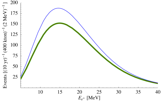
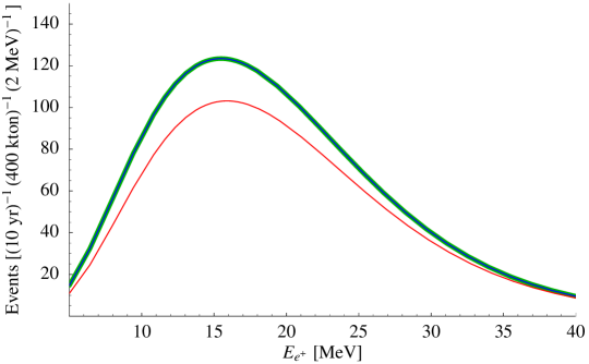
(a)                                                                                (b)

Figure 1: The neutrino differential event number vs. the predicted one using the future-observed supernova rates. The observed differential event number is plotted in green and corresponds to the differential flux folded with the cross section using our above projection. The red (blue) curves correspond to the predicted differential flux assuming $\Lambda$CDM, $\Omega_{M}=0.3$ and $w=-1$, (SCDM, $\Omega_{M}=0.3$ and $w=0$) cosmology. The true cosmology is $\Lambda$CDM in (a) and SCDM in (b). Normal hierarchy is assumed and the input values for the neutrino fluxes are given in Table 2.

III Measuring the Core Collapse Rate via SN Observatories

Before considering the details of the direct observation of core collapse rate, we first compare the present and future methods of SN-rate determination and explain why we need a SN survey. Our proposal relies on the fact that the cosmological parameters enters differently in the measurements of the supernova density and the differential neutrino flux. In this way the dependence on the largely unknown shape of the SN comoving rate cancels in the predicted neutrino flux. At the same time the latter remains rather sensitive to the cosmological parameters. The validity of the above statement depends on the experimental method by which $R_{\rm SN}(z)$ is extracted. In the following we discuss the present and future methods for extraction of $R_{\rm SN}(z)$. We shall argue that future, more direct, measurements are what is required to make our proposal a possibility.

III.1 Present knowledge of the SN rate

The conventional observation of the SN rate relies on measurements of light emitted from galaxies, mostly in the UV (see e.g GALEX for a recent compilation of the data). Even though a lot of effort is dedicated to improve the precision of these measurement, $R_{\rm SN}$ still suffers from rather large uncertainties. Furthermore the above measurements are not very useful for our proposal since the sensitivity to the cosmological parameters is lost when they are used in combination with the SRN flux Ando . In the case of (UV) light measurements, the comoving rate would be proportional to the observed flux, $L^{\rm obs}$, according to the relation

$$L(z)^{\rm obs}\propto\frac{R_{\rm SN}(z)}{1+z}\frac{dV}{dz}(w)\frac{1}{d_{L}(w)^{2}}.$$ (5)

One clearly see that $R_{\rm SN}$ and the factors carrying the cosmological information enter exactly in the same combination as in Eq. (1). Thus the predicted SRN differential rate, in terms of the SN core collapse rate, is given by ${\Phi^{\nu}}\propto\int dz\,L^{\rm obs}\,{dN^{\nu}/d\epsilon},$ which is, to leading order, cosmology independent. Methods which rely on comparison between light flux measurements and neutrino flux measurements are not useful, since the resulting dependence on cosmology is very weak.

Forthcoming SN observatories will have the power to record an ${\cal O}(5000)$ CC SNe per year (see also  SNAP ) and will yield a significant improvement in the measurement of $R_{\rm SN}(z)$ Ando ; GalMa ; OdaTot ; Dahl . In this case the extracted comoving SN rate is inferred by using Eq. (6). One can repeat the above manipulations but in this case the cosmology does not cancel in the expression for the predicted SRN differential flux. This can be easily understood since the counting of explosions is a measurement of density. When combined with a measurement of a flux the resulting expression is still cosmology dependent, as shown explicitly in (4).

It is interesting to note that the mere comparison of the SN rate indirectly inferred from measurements of SFH with the direct one contains some cosmological information, even without the need of measuring the flux of the SRN. The problem with such an analysis is two-fold. First of all, the determination of SFH is not very precise and it is subject to large uncertainties. For instance the measurements of UV light are subject to large dust absorption factors (so that large corrections must be applied in order that the UV and IR data agree GALEX ). Thus the resulting uncertainties are large. Secondly, one needs to assume that the SN explosion rate is directly proportional to the SFH [see $\kappa$ in Eq. (6)] and the redshift dependence of the proportionality constant has to be modeled (a constant is chosen as a first approximation). It is hard to see how this assumption will be independently tested and the proportionality coefficient accurately measured in the near future.

The situation is different when using the neutrino signal. Moreover, unlike in the case of the star formation rate, the physical mechanism of neutrino emission from CC SNe is in principle better understood. Clearly in terms of light spectra and emission the CC SNe are much richer and show strong dependence on the progenitor type (not to mention the open questions regarding the explosion mechanism). However, one should bear in mind that the photons carry away only 1% of the emitted energy while 99% of the energy is released in neutrinos. Thus the above uncertainties affect neutrino emission in a less dramatic way. Simulations and theoretical arguments seem to imply that, in terms of the neutrino flux, the CC SNe are much more universal than in terms of the emitted light Bur ; LL ; Buras1 ; Buras2 ; Review . This is naturally expected since neutrino emission mostly depends on the physics of the collapsing iron core reaching the Chandrasekhar mass, deep inside a huge star. Very crudely the above picture was already confirmed by the observation of the 1987a SN neutrinos. Clearly, the details of the observed spectra shows some puzzling features RafMir ; Lunar ; Review ; SN1987 which call for more data. We expect that in the future substantial theoretical and experimental progress will be made to further improve the understanding of the emitted neutrino spectra.

III.2 Analysis of the SN rate from direct observation

We shall now discuss in more detail the future observation of the core collapse supernova rate. Our main aim is to extract the significance of our proposal. To do this, we need to estimate the core-collapse SN rate per red shift bin that a SNAP-like survey will observe. Furthermore, in order to correctly assign the statistical uncertainties and estimate the systematics, we should have a reasonable idea regarding the detection efficiency and the SN light extinction. We would like also to check that our method, in a realistic case, remain fairly insensitive to the specific form of $R_{\rm SN}$, as it was in the previous idealized case. The above issues are addressed in two steps as follows:

• We assumed two different comoving core collapse rates $R_{\rm SN}(z)$ and for each one the expected explosions per red shift bin, $R_{\rm SN}^{\rm obs}(z)$, was computed in both the $\Lambda$CDM and SCDM cosmologies.

• We extracted the detection efficiencies and the dust extinction effects by using the SNOC Monte-Carlo simulation package for high-$z$ supernova observations SNOC . We applied a detection strategy and optical sensitivity as given in the SNAP specification. Since the total acceptance depends on cosmology, this was done for the two underlying cosmologies. Moreover we simulated samples of SNe using different dust properties in order to estimate (part of) the systematic uncertainties.

With the above information at hand, we combined the two pieces of uncertainties into an overall uncertainty on the SN counts per redshift bin. This would later be combined with the projection for the SRN spectral measurements in order to estimate the significance of our method.

We shall now describe each of the above items in more detail. We start with step (ii) which is related to the estimation of SNAP acceptance. We used filters spanning from B to near-infrared (NIR), H-band. We required the following specifications for a full detection (and tagging) of a core collapse SN: one point on the light curve, 4 rest-frame days before the peak-luminosity in at least one filter band, and 10 points on the light curve in all the bands. We derived the efficiencies for two scanning strategies, a 4-day and an 8-day one, with limiting detection magnitudes of 25 and 28 respectively (the 8-day search is deeper). For simplicity we only focused on detection of Type-II SNe which accounts for roughly 80% of the total number of core collapse SNe. For each 0.1 red shift bin, we simulate 1000 explosions so that the statistical uncertainties in estimating the efficiency are of ${\cal O}$(3%) and will be neglected in the total error.

To estimate the systematic uncertainties we only focus on the dependence upon dust properties. We extracted the central value of the efficiency by using a “high” dust model with selective extinction $R_{V}=4$, a typical value for starburst galaxies. Indeed recent observations suggest that a sizable number of CC SNe are dust extincted. However we also repeated the analysis with two other dust models with lower and higher dust content (with $R_{V}=3.1$ and $4.9$ respectively). The spread of the efficiencies computed in these different models should give an idea of the size of systematic uncertainties introduced by dust (as in SNOC, we do not take into account any $z$-dependent dust evolution). Given the recent progress in understanding dust properties of high redshift galaxies we can assume that our knowledge on dust extinction will be significantly improved in the next 10-15 years, and used to estimate better the efficiency. Thus in the following we will use as an estimate of the systematic uncertainties on the efficiency the spread of the above models reduced by a factor of $2$.

Another reason for the need to estimate the efficiency is that it depends on the underlying cosmology. As a first approximation one can think about it as $\epsilon(w,z)=\epsilon(d_{L}(w,z))$ and it decreases for high redshifts. As we will show below, the dependence on the cosmology in the predicted SRN flux will be $\propto 1/\left[d_{L}^{2}\,\epsilon(d_{L})\right]$ (see Eq. (12)) and we therefore verified that the efficiency does not significantly reduce the sensitivity to the cosmological parameters. In Fig. 2(a) (2(b)) we plot the efficiency, $\epsilon(w,z)$, per 0.1 redshift bin for the $\Lambda$CDM, in red, and SCDM, in blue, cosmologies using 4-day (8-day) scanning strategy respectively. In all cases the error bars corresponds to the systematic error as explained above.

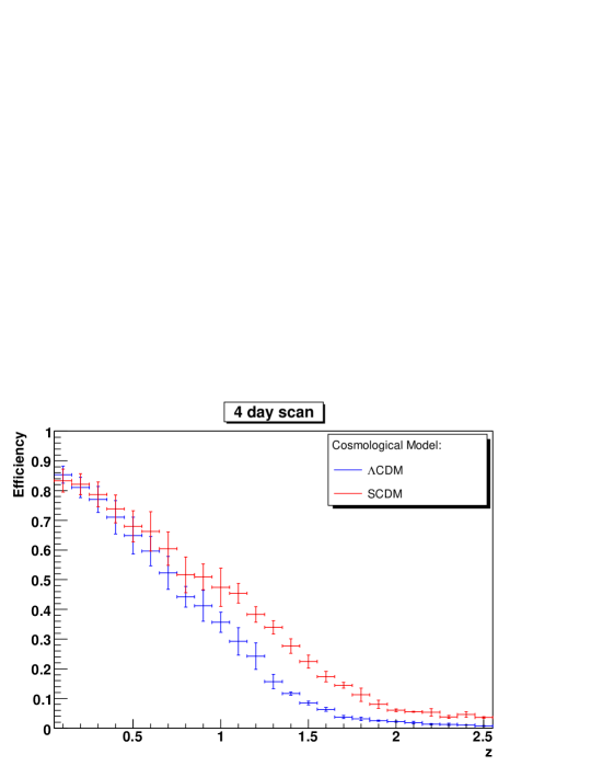
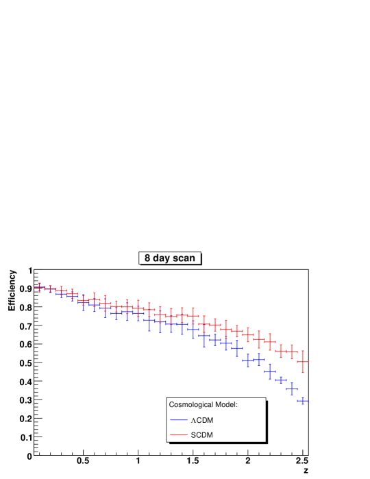
(a)                                                                                (b)

Figure 2: The efficiencies for observation of Type-II SNe in $\Lambda$CDM (SCDM) cosmology based on 4 days (a) and 8 days (b) scan strategies. For our projections we used the best fit GALEX values GALEX ($\alpha,\beta$ in table I) for $R_{\rm SN}$.

Parameter	Value
$\kappa\,\times M_{\odot}$	0.013
$z_{p}$	1
$\alpha$	0.5
$\beta$	2.5
$\Phi(1)\,$yr Mpc/M⊙	$10^{-1.05}$
$\alpha^{\rm SCDM}$	0.71
$\beta^{\rm SCDM}$	3.05
$\Phi(1)^{\rm SCDM}\,$yr Mpc/M⊙	$10^{-0.84}$

Table 1: Inputs related to the SN rate, used in our analysis. The parameters are set to their median values since they are only required in order to produce the mock distribution etc. The values are taken from Ref. GALEX . Parameters that appear with an SCDM upper-subscript have been readjusted for an SCDM cosmology.

We now discuss item (i), i.e., our estimate of the true core collapse explosion rate per 0.1 redshift bin. As explained above, we expect that the dependence on the specific parameters of $R_{\rm SN}$ should be weak for the overall fit. Thus in most of our analysis we shall just use the median values for the SN rate. A good parameterization of $R_{\rm SN}$ is GalMa ; OdaTot

$$R_{\rm SN}(z) = \kappa\frac{2^{1\over 5}\Phi(z_{p})}{\left[\left({1+z_{p}\over 1+z}\right)^{5\alpha}+\left({1+z_{p}\over 1+z}\right)^{5\beta}\right]^{1\over 5}}\;.$$ (6)

The present knowledge of the numerical values for the various parameters in (6) is given in Table 1. The way the SN rate parameters, in particular the exponents $\alpha$ and $\beta$ which characterize the shape of the star formation rate, are extracted from data depends on the underlying cosmology assumed GALEX ; CosTrans . Thus as a confirmation of our claim we also repeat part of the analysis for an alternative values of $\alpha,\beta$ and $\Phi(1)$, denoted as $\alpha^{\rm SCDM},\beta^{\rm SCDM}$ and $\Phi(1)^{\rm SCDM}$. These were extracted from the GALEX data GALEX assuming SCDM universe à la Ref. CosTrans . We used the combination of Eqs. (3) and (6) for each of the above four cases in order to derive our estimate for the amount of visible explosions. This is done for one year of SNAP and $15{\rm\,sq.\,deg.}$ of effective sky coverage for 4-day scanning combined with a $1{\rm sq.\,deg.}$ coverage of an 8 days scanning. The expected number of SNe events observed by SNAP, per red shift bin, is then given by

$$\bar{N}^{\rm SN}(w^{T},z)={R_{\rm SN}\over 1+z}\,{dV\over dz}(w^{T},z)\,{\Delta\Omega}\,\Delta z\,\tau\,\epsilon(w^{T},z)\,,$$ (7)

where $\Delta\Omega$ is the solid angle in steradians taken to be $\Delta\Omega\simeq 15(1)$ ${\rm sq.\,deg.}$ for the 4-day (8-day) respectively, $\Delta z=0.1$, $\tau=1$yr stands for the SNAP running time, $\epsilon(w,z)$ is the efficiency discussed above and the upper index $T$ in $w$ is just to emphasize that they correspond to the true cosmological parameters which are not directly accessible to the experimentalist but will be used for our projections.

Given the observed explosion number $\bar{N}^{\rm SN}$ and the efficiency $\epsilon(w,z)$, the estimated number of SN explosion, $N^{\rm SN}(w^{T};w,z)$, is given by

$$N^{\rm SN}(w^{T};w,z)=\bar{N}^{\rm SN}(w^{T},z)/\epsilon(w,z)\,.$$ (8)

Note that $N^{\rm SN}(w^{T};w,z)$ depends on the underlying true cosmology. The error on $N^{\rm SN}$ is easily determined by remembering that the SN explosion is a Poisson process and the detection is a binomial process. Thus the observed number of SN is still Poisson distributed, being a convolution of a Poissonian and a binomial distributions. Combined with our estimated efficiency, the error assigned to each bin is

$$\delta N^{\rm SN}/N^{\rm SN}\sim\sqrt{1/\bar{N}^{\rm SN}+(\sigma_{\epsilon,syst.}/\epsilon)^{2}}\,.$$ (9)

We used the above to simulate the core collapse observed value (after the corrections due to the imperfect efficiencies) for the case in which the true cosmology is $\Lambda$CDM, $w^{T}=-1$. The errors were estimated according to Eqs. (8,9). We further computed the same observed rate for the case in which the true cosmology is SCDM, $w^{T}=0$, using the $R_{\rm SN}$ parameters $\alpha^{\rm SCDM},\beta^{\rm SCDM}$ and $\Phi(1)^{\rm SCDM}$, allowing us to check the robustness of our method. As expected SNAP , our analysis indicates that future SN observatories such as SNAP will have the power of collecting $\cal O$(5000) core collapse events in 1-2 years of running.

We finish this part of discussion by remarking that a similar analysis may also be possible in the future by using the information on the type Ia SN explosions rate. Type Ia SNe are less abundant but are brighter and they occur in regions of the galaxies with moderate amount of star formation activity (since they originate from “old” progenitors) thus less dusty. Their detection is much easier, and the efficiency is less prone to systematic uncertainties due to dust. However their tracking of the SFH curve is delayed due to the time needed to bring this kind of systems to the explosion stage (accretion of gas on a white dwarf in a dwarf-giant tight binary system). A measurement of the Type Ia explosion rate might be used in the future as an additional source of data, to independently cross check the $R_{\rm SN}(z)$ directly inferred from CC SN observations, even if the Type Ia delay time has to be better studied and measured GalMa ; OdaTot ; Dahl .

IV SN neutrinos, spectra and detection

In this section we focus on the detection possibilities of the SRN signal. Our main aim is to estimate the possible precision that can be reached by future neutrino experiments. This section is divided into two parts. We first discuss the future neutrino detectors (Mt Cherenkov detectors enriched by GdCl₃ and also 100Kt liquid Argon ones) and discuss their ability to observe the SNe diffuse neutrino flux. Then we consider the uncertainties related to the flux and spectra of the neutrinos emitted from CC SNe. We discuss the possibility of constraining some of the related unknowns via future observation of nearby SN bursts.

IV.1 Observation of the SN diffuse neutrino flux

Despite great interest in observing the SRN flux, present experiments have not been able to detect these neutrinos coming from the edge of our Universe. They only put an upper bound on the corresponding flux, the strongest one coming from Super-Kamiokande, with a rather high threshold $\sim 18\,$MeV BoundFlux . Given the uncertainties in the star formation history and in the neutrino spectra and mass hierarchy, a sharp prediction for the flux is difficult to obtain Ste ; Str ; BeSt ; Lunar . Nevertheless the above bounds already provide a valuable constraint on the relevant parameters. It is clear however that in order to make a significant progress towards an observation of the SRN flux a dramatic improvement is required. Here we shall focus on future Mt Cherenkov detectors (such as UNO UNO , Hyper-Kamiokande HyperK or MEMPHYS MEMPHYS ) which, due to their larger volumes, will have better sensitivities. The most promising detection channel is through the inverse beta decay induced by a SN anti-neutrino $\bar{\nu}_{e}p\rightarrow e^{+}n$. As was shown by Beacom and Vagins in the GADZOOKS! proposal GAD , once the water detectors are enriched by a small amount of GdCl₃, the sensitivity to the subsequent neutron capture is increased by several orders of magnitude, allowing for significant reduction of solar, spallation and invisible muon backgrounds BoundFlux ; GAD ; Fogli . The dominant backgrounds are from atmospheric and reactor anti-neutrinos. If the Mt detector is located in a reactor-rich zone the threshold could be lowered down to 10 MeV, while in a more reactor-free location the threshold could be further lowered down to 6-7 MeV GAD ; Fogli .

In the following we aim towards estimating the precision with which the SRN differential event rate $d\Phi^{\nu}/dE$ could be determined by the future experiments. The differential flux, $dF/dE$, is determined via Eq. (1). Given the prediction for the differential flux, the spectrum for the predicted number of events is

$$\Phi^{\nu}(E,\Omega_{\Lambda})\simeq\frac{dF}{dE}(E,\Omega_{\Lambda})\,\sigma(E)\,N_{p}\,\tau\Delta E\,,$$ (10)

where $\sigma$ is the cross section for the inverse beta decay, which roughly grows like $E^{2}$ Vog (in our actual computation we used the phenomenological formula of Vog ), $N_{p}\sim 3\times 10^{34}$ is the number of protons in a 0.4 Mt detector and $\tau\sim 10$yr is the detector run time. Note that $\Phi^{\nu}$ is a function of cosmological parameters, as explained above.

The mean SRN flux estimate is based on a bin by bin analysis, for $2$MeV bin size. The number of SRNs per energy bin, $N_{s}(\Omega_{\Lambda},E)$, in a real experiment will be obtained after subtracting the relevant backgrounds from the measured counts $N_{t}$. In our analysis, we take the error as

$${\Delta N_{s}\over N_{s}}\simeq\frac{\sqrt{N_{t}+N_{b}}}{N_{t}-N_{b}}\,,$$ (11)

for each energy bin, where we used the numerical values given in GAD ; Fogli for the estimated value of the background events $N_{b}(E)$, which are mainly due to the $\bar{\nu}_{e}$ atmospheric flux and the invisible muon flux. We considered both the case of Hyper-Kamiokande in which the lower threshold is determined by the reactor $\bar{\nu}_{e}$ background and the case of a “cleaner” environment, where the lower threshold can be lowered down to roughly 6MeV. In Figs. 3(a) (3(b)) we plot our projections for the observed event number in the $\Lambda$CDM (SCDM) case in 10 years for a 0.4 Mt detector. Blue (red) error bars do (not) include reactor backgrounds; errors are assumed to be statistical.

We finish this part by mentioning that, while in the above we focused on Mt Cherenkov water detectors, there are other promising proposals in the future neutrino program for building ${\cal O}$(100kt) liquid Argon/liquid scintillator detectors ALD ; LENA . These kinds of detectors will be able to observe tens of SRN events in their lifetimes. In the case of Argon detectors, the sensitivity is better for the neutrino flux than for the anti-neutrino one Cocco . Thus a combination of the two types of detectors would provide a better control of systematics and an improvement in the understanding of the core collapse SN physics, as briefly discussed below.

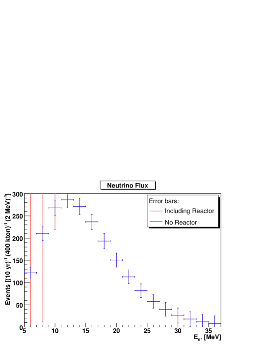
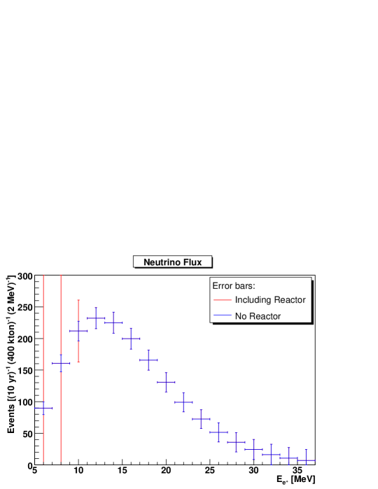
(a)                                                                                (b)

Figure 3: The expected number of events, per 2 MeV energy bin, in a 10-year run of a 0.4 Mt detector, for the $\Lambda$CDM case (a) and for the SCDM case (b). Errors are statistical and include the background subtraction (11). Also blue (red) error bars (do not) include the reactor anti-neutrino background.

IV.2 Core collapse neutrino spectra

The last required step in order to extract the significance of our method is related to estimating the emitted neutrino spectra, ${dN(\epsilon)}/{d\epsilon}$. As discussed above, the data from the SN observatories can be used to derive an estimate for the SN rate (7,8). Using this piece of information and a knowledge of the neutrino spectra we can derive a prediction for the neutrino flux using Eqs. (10) and (11):

$$\frac{dF}{dE}(w^{T},w,E)\propto\int_{0}^{z_{max}}\frac{\bar{N}^{\rm SN}(w^{T},z)}{\epsilon(w)}\left.\frac{dN^{\nu}(\varepsilon)}{d\varepsilon}\right|_{\varepsilon=(1+z)E}\;\frac{1}{d_{L}^{2}(w)}dz\,,$$ (12)

where $\bar{N}^{\rm SN}(w^{T},z)$ is the one measured in the SN survey (see Eq. (7)).

In order to have a reliable prediction of the SRN flux, we need to have the neutrino spectrum from a single SN, $dN^{\nu}/dE(E)$, somewhat under control. Core collapse dynamics and its explosion mechanism is one of the most challenging and intriguing questions in modern astrophysics (see Review for a recent review). The core collapse mechanism is thought to be known, at least roughly, while the explosion is still a mystery. This is also reflected in the theoretical understanding of the emitted neutrino spectra, which is known only to a rough accuracy. However it is important to note that as a first approximation the above uncertainties have very little to do with the neutrino dynamics, since the iron CC and the conditions that create the “neutrinospheres”, whose surface emission accounts for roughly 99% of the energy released in the SN cooling, is thought to be understood Bur . Moreover the above predictions were tested by the observation of neutrinos from SN 1987a. As mentioned above it is largely accepted KRJ ; Review that the neutrino spectra can be well approximated by a pinched Fermi-Dirac distribution

$$\frac{dN^{\nu}(\epsilon)}{d\epsilon} = \cos^{2}\theta{\cal F}(\epsilon,\bar{E}_{\bar{\nu}_{e}},\beta_{\bar{\nu}_{e}},L_{\bar{\nu}_{e}})+\sin^{2}\theta{\cal F}(\epsilon,\bar{E}_{\nu_{x}},\beta_{\nu_{x}},L_{\nu_{x}})\,;$$ (13)

$${\cal F}(\epsilon,\bar{E}_{i},\beta_{i},L_{i}) = {L_{i}\over\bar{E}_{i}^{2}}\,{(\beta_{i}+1)^{\beta_{i}+1}\over\Gamma(\beta_{i}+1)}\,\left({\epsilon\over\bar{E}_{i}}\right)^{\beta_{i}}e^{-(\beta_{i}+1){\epsilon\over\bar{E}_{i}}}\;.$$ (14)

where $\bar{E}_{i},L_{i},\beta_{i}$ corresponds to the average energy, flux and the pinching parameter of the electron anti-neutrino, $\bar{\nu}_{e}$, and the muon/tau anti-neutrinos, $\bar{\nu}_{x}$. $\theta$ is the relevant mixing angle which is determined by matter effects in the SN mantle Mix .

Parameter	Value	$\sigma$	Ref.
$\bar{E}_{\nu}^{\rm exp}/$MeV	12.2	0.75	central value RafMir , future uncertainty estimated
$\beta_{\nu}^{\rm exp}$	3	0.25	central value RafMir , future uncertainty estimated
$L_{\nu}^{\rm exp}/10^{52}{\rm erg}$	5.5	0.75	central value RafMir , future uncertainty estimated
$\bar{E}_{\bar{\nu}_{e}}^{\rm th}/$MeV	15	-	KRJ ; Ando ; Review
$\beta_{\bar{\nu}_{e}}^{\rm th}$	3	-	KRJ ; Ando ; Review
$L_{\bar{\nu}_{e}}^{\rm th}/10^{52}{\rm erg}$	5.5	-	KRJ ; Ando ; Review
$\bar{E}_{\nu_{x}}^{\rm th}/$MeV	16.5	-	KRJ ; Ando ; Review
$\beta_{\bar{\nu}_{x}}^{\rm th}$	3	-	KRJ ; Ando ; Review
$L_{\bar{\nu}_{x}}^{\rm th}/10^{52}{\rm erg}$	5.5	-	KRJ ; Ando ; Review

Table 2: Inputs used in our neutrino spectra analysis. For our actual analysis we use the effective spectra (given in the first three rows) as measured on earth using an effective single generation case RafMir . We use our projection to estimate the future error on the relevant parameters. The parameters (given in the following six rows) for the three neutrino case are used only for the illustration plots (1) and the ones which demonstrate the difference between the normal and inverted hierarchy cases (4). Thus for this part of the analysis we only use mean values.

Before discussing the uncertainties related to the spectral shape, we would like to consider how the the different neutrino mixing and mass hierarchy affect our analysis through matter effects. The detection process is sensitive only to the flux of incoming electron anti-neutrinos. Consequently, to include contributions to the flux from the muon/tau and electron anti-neutrinos we use the corresponding average energy and the other spectral parameters in the expression for the anti-neutrino spectrum, and include mixing factors. As discussed in Refs. Mix ; LS , the relation between the $\bar{\nu}_{e}$ spectrum observed on Earth to the various neutrino spectra at production depends critically on whether the neutrino mass hierarchy is normal or inverted. If normal then strong matter effects cause the $\bar{\nu}_{e}$ at production to emerge from the stellar surface as the lightest eigenstate $\bar{\nu}_{1},$ with electron component $|U_{e1}|^{2}\simeq 0.69$ PDG (thus in this case $\cos^{2}\theta\sim 0.69$). The small mixing of the electron with the third eigenstate $|U_{e3}|^{2}\ll 1$ allows an equivalent two-flavor picture, with the result that anti-neutrinos produced in the supernova as $\bar{\nu}_{x},\;x=\mu\ \mbox{or}\ \tau$ will be received at Earth as $\bar{\nu}_{e}$ with probability $1-|U_{e3}|^{2}\simeq 0.31$, and with energies corresponding to the $\bar{\nu}_{\mu}$/$\bar{\nu}_{\tau}$ spectrum at production. For the case of the inverted hierarchy, $\bar{\nu}_{e}$’s produced in the supernova emerge as the lightest mass eigenstate now $\bar{\nu}_{3}$. For $\sin^{2}2\theta_{13}\lower 2.58334pt\vbox{\hbox{$\buildrel\textstyle<\over{\sim}\ $}}10^{-6}$, the resonance is non-adiabatic and there is complete conversion $\bar{\nu}_{3}\rightarrow\bar{\nu}_{1}$. This case then is the same as for the normal hierarchy. The adiabatic case, $\sin^{2}2\theta_{13}\lower 2.58334pt\vbox{\hbox{$\buildrel\textstyle>\over{\sim}\ $}}10^{-4}$, is very different: the original $\bar{\nu}_{e}$’s remain as $\bar{\nu}_{3}$ when emerging from the stellar surface, with a negligible contribution to the $\bar{\nu}_{e}$ flux at Earth. The entire $\bar{\nu}_{e}$ flux at Earth then corresponds to the original $\bar{\nu}_{x}$ produced in the supernova. For intermediate values of $\sin^{2}2\theta_{13}$, the situation is of course more complicated. We assume therefore that before the end of the lifetime of our detectors the neutrino mass spectrum will be determined by long-baseline neutrino oscillation experiments. In this context, we also note that Earth matter effects have been shown to modify the observed fluxes and spectra on Earth Earth . Since however the hierarchy in the average energies between the $\bar{\nu}_{e}$ and the other flavors is mild, this effect is expected to be subdominant and is neglected in our analysis RafMir (see however Lunar ).

To present the related effects, we considered here the predicted neutrino flux for the two extreme cases. The normal hierarchy case was already shown above (see Figs. 1). The other extreme is related to the inverted hierarchical case for the a large $\theta_{13}\,.$ For each of the above cases we compared the predicted neutrino flux, inferred by the SN observation data, assuming the two different cosmologies with the “observed” flux. Here in Fig. 4 we only show the case in which the true cosmology is $\Lambda$CDM, the other (with SCDM true cosmology) being similar. To produce the plot we use the relevant mean value parameters for the neutrino spectral shape shown in Table 1. We did not find it instructive to repeat the analysis below for the various possible values of $\theta_{13}$ and the mass hierarchy. The rest of our analysis below is applied for the normal hierarchy case but it would be straightforward to repeat it for any values of the neutrino flavor parameters (again assuming that the neutrino flavor parameters are known). Furthermore, since in the inverted hierarchical case with a sizable $\theta_{13}$ the neutrino spectrum is typically harder, the significance of our method increases. Thus in this sense by analyzing the normal hierarchy case we give a conservative estimate for the extracted significance.

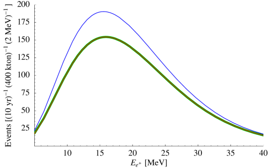
Figure 4: The same as in Fig. 1(a), but for neutrino masses with an inverted hierarchy.

We now turn to consider the uncertainties on the spectral parameters $\beta$, $L$ and $\bar{E}$. At present it is hard to theoretically estimate the relevant uncertainties assigned to the above parameters. The theoretical prediction for the neutrino spectra is subject to a continuing research which largely relies on computer simulations theory ; Bur ; LL ; Buras1 ; Buras2 ; Review and therefore we expect a significant improvement in the relevant time range of roughly 10-15 years from now. Furthermore, in this time range future neutrino detectors will have improved ABY sensitivity to nearby non-galactic SNe explosions, which occur much more frequently. Adding to that the hope of having another nearby SN explosion, we allowed ourselves the following treatment for the related uncertainties. We take our guidelines from the present experimental knowledge of the spectral parameters based on the work by Mirizzi and Raffelt RafMir . In that work the observed neutrino spectra from SN1987a is matched to the above theoretical formula, Eq. (14). Since the discussed flux is the one observed on the Earth, there is no need to parameterize the matter effects in the SN mantle. We use the fit of Mirizzi and Raffelt to extract the mean values for the parameters. At present, the uncertainties on the parameters is very large and not very useful. With 10-15 years of the Mt detector one may hope to roughly triple the statistics ABY . Furthermore, in the case of a local SN burst at least 10000 neutrino event will be observed which will allow for a precise determination of the above parameters.

It is not yet clear how universal are the above parameters which may slightly vary from one SN to another (mostly the luminosity; see discussion below). Thus for our projections we assume a factor of 4 reduction in the uncertainties which would be hopefully feasible due to theoretical, experimental or a combined progress in the field. In this approach the ultimate “irreducible” uncertainties on the spectral parameters will be determined by their dependence on the SN progenitor characteristics. This dependence has been investigated in Bur (see also Review ; Buras1 ; Buras2 ) and found to be generally “small”. Here we keep the larger between the 25% error uncertainty described above and the spread found from simulation of the progenitor mass dependence. These errors are summarized in Table 2.

We find that varying the pinching parameter $\beta$ and the average energy $\bar{E}$ do not significantly affect the fit and, when marginalizing on these, the preferred value for the cosmological parameters are rather stable. However a strong dependence is found on the value of the luminosity. Thus instead of marginalizing over the luminosity (which would lead to a weak constraint) we plot the CL as a function of both $w$ and neutrino luminosity. In Fig. 5(a) (5(b)) we plot the CL in the $\Delta L/L$ vs. $w$ plane, for the $\Lambda$CDM case assuming 10 years of Mt detector with reactor neutrino background present (absent). In Fig. 6 we show the corresponding plot for the case when a different ansatz for the comoving SN rate is used, as explained in Sec. III.2. The above analysis assumes, however, that the uncertainty of the luminosity is evenly distributed around the projected mean value. In particular it is evident from the above plots that for lower values of the luminosity the ability to distinguish between the two cosmology becomes much worse.

However, one should expect that the neutrino luminosity will be, to some extent, correlated with the progenitor star mass. This has been also pointed out by simulations of the progenitor mass dependence. In particular, simulations indicate that the luminosity tends to increase with progenitor mass Buras1 ; Buras2 . Since the progenitor mass function is a rapidly monotonically decreasing function, it is clear that the luminosity function would be concentrated around the lowest possible value with an asymmetric spread. We used Buras1 ; Buras2 to estimate that the spread in luminosity below the mean value is roughly 5% while 25% above the mean value. In that case the fit improves when the asymmetric distribution is assumed as shown in Figs. 7(a) and 7(b), which should be compared to Figs. 5(a) and 5(b) respectively. A more careful analysis of the dependence of luminosity on the progenitor mass is required, and can be improved when better information becomes available. Here, this rough estimate demonstrates the possibility of future improvements to our analysis.

We finish this part by mentioning that in the above we neglected, for simplicity, various non-linear effects inside the SN core which affect the neutrino spectrum, such as propagation of a shock-wave shock and also the presence of turbulence .

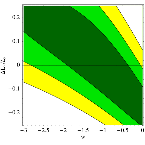
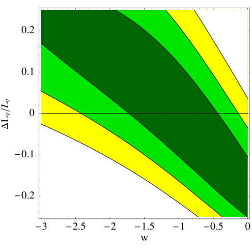
      (a) Reactor background present                        (b) Reactor background absent

Figure 5: The allowed region in $w\,-\,L_{\nu}$ plane for $w=-1$ case. The dark green, light green and yellow region roughly corresponds to 68%, 95%, 99.7% CL. This assumes a 10 year run of a Mt detector. Fig. (a) includes the presence of a reactor anti-neutrino background, while (b) do not.

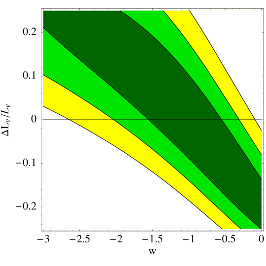
Figure 6: The same as Fig. 5(b), but with a different ansatz for $R_{\rm SN}$ ($\alpha=\alpha^{\rm SCDM}$, $\beta=\beta^{\rm SCDM}$).

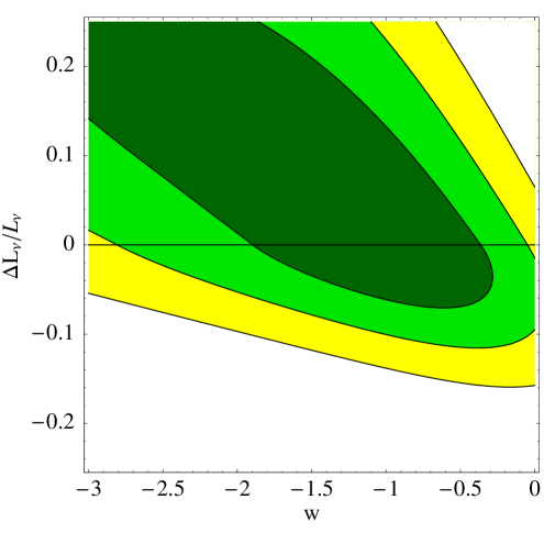
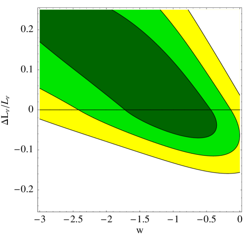
      (a) Reactor background present                        (b) Reactor background absent

Figure 7: The same as in Figs. 5(a,b), but taking a highly asymmetric error on the luminosities, due to the rapidly decreasing star mass function.

V Discussion

We have demonstrated that the observation of supernova relic neutrinos (SRNs), when combined with improved measurements of the past supernovae explosion rate, has the potential to probe the expansion history of the Universe. The cosmology dependence in our proposal enters through a weighted integral over red shift of the luminosity distance squared (weighted by the supernova rate and the neutrino spectra), and hence differs from luminosity distance measurements of Type Ia supernova observations.

The prospect of probing fundamental cosmological parameters using a different probe other that photons is very exciting. Such measurements open the possibility of sensitivity to unknown new physics that distinguish photons from other kind of particles. One such example is the case of photon-axion mixing axion (or more generally, mixing of photon with any other light particle) where some of the original photon flux is converted to a flux of invisible particles. While it is known that the current data regarding the acceleration cannot be solely explained by such an effect w , it can still be significantly affected by it axion ; w . For instance, it can drive the equation of state parameter, $w$, to rather low values, below $-1$, or to high values, above $-0.5$.

It is known that the supernova data alone allows for very low values of $w$ (even values below $-2$ are allowed) since it is highly degenerate in the $\Omega_{M}-w$ plane (even though, with a larger sample and a wider redshift range, the supernovae data by themselves will be able to break this degeneracy; see e.g. the recent release of SNLS SNLS ). In the future it will be very interesting to compare the constraints on $w$ from SNe with other experimental results, to look for systematic biases or non-standard physics, especially since other surveys have started to probe $w$ as well; see e.g. new for a recent discussion. It is noted in that context that our signal, which is driven by the neutrino flux, is subject to very different kinds of systematic biases and is affected by very different kinds of new physics effects.

We remark that the numerical closeness of the neutrino mass and the dark energy scale has recently attracted a lot of interest in the possibility that these two are related Nu . If this is indeed the case, it could be that the Universe “seen” with neutrinos is very different from the one probed via photons MiniZ . In that sense, even though our method cannot compete with the precision of optical methods, it is complementary to the ones already proposed SNAP ; Others .

In the case where the above analysis will not reveal deviations from the expected results (based on optical observation) one can apply a similar analysis in order to improve our knowledge regarding the neutrino spectra. Setting the cosmological parameters to their values obtained from the future global fit and combined these with the observed diffuse neutrino flux will allow one to extract the values of the parameters determining the SN neutrino energy spectra.

We finally comment that our method does not rely on the construction of a dedicated new experiment but rather on combining data from experiments that are likely to be built for other reasons.

References

- (1) S. Perlmutter et al. [Supernova Cosmology Project Collaboration], Astrophys. J. 517, 565 (1999) [arXiv:astro-ph/9812133].
- (2) A. G. Riess et al. [Supernova Search Team Collaboration], Astron. J. 116, 1009 (1998) [arXiv:astro-ph/9805201].
- (3) D. N. Spergel et al. [WMAP Collaboration], Astrophys. J. Suppl. 148, 175 (2003) [arXiv:astro-ph/0302209]; G. Hinshaw et al., arXiv:astro-ph/0603451; D. N. Spergel et al., arXiv:astro-ph/0603449.
- (4) W. J. Percival et al. [The 2dFGRS Collaboration], Mon. Not. Roy. Astron. Soc. 327, 1297 (2001) [arXiv:astro-ph/0105252].
- (5) D. J. Eisenstein et al., arXiv:astro-ph/0501171.
- (6) S. W. Allen, A. C. Fabian, R. W. Schmidt and H. Ebeling, Mon. Not. Roy. Astron. Soc. 342, 287 (2003) [arXiv:astro-ph/0208394].
- (7) C. K. Jung, arXiv:hep-ex/0005046.
- (8) K. Nakamura, Int. J. Mod. Phys. A 18, 4053 (2003).
- (9) L. Mosca, Nucl. Phys. Proc. Suppl. 138 (2005) 203; J. E. Campagne, M. Maltoni, M. Mezzetto and T. Schwetz, arXiv:hep-ph/0603172.
- (10) J. F. Beacom and M. R. Vagins, Phys. Rev. Lett. 93, 171101 (2004) [arXiv:hep-ph/0309300].
- (11) See http://destiny.asu.edu/ for more details.
- (12) See http://serweb.oamp.fr/perso/tresse/moriond06/talks/amara_moriond06.pdf for some details.
- (13) JEDI white paper submitted to the Dark Energy Task Force (invited presentation during the DETF meeting on June 30, 2005), astro-ph/0507043; See http://jedi.nhn.ou.edu/n for more details.
- (14) See http://www.lsst.org/lsst_home.shtml for more details.
- (15) See e.g. P. Nugent [SNAP Collaboration], Prepared for 2nd Tropical Workshop on Particle Physics and Cosmology: Neutrino and Flavor Physics, San Juan, Puerto Rico, 1-6 May 2000; Science proposal to the DOE and the NSF Dec (2000); See snap.lbl.gov/ for more details.
- (16) N. W. Halverson et al., Astrophys. J. 568, 38 (2002) [arXiv:astro-ph/0104489]; C. B. Netterfield et al. [Boomerang Collaboration], Astrophys. J. 571, 604 (2002) [arXiv:astro-ph/0104460]; Astrophys. J. 396, L1 (1992); A. Balbi et al., Astrophys. J. 545, L1 (2000) [Erratum-ibid. 558, L145 (2001)] [arXiv:astro-ph/0005124].
- (17) L. E. Strigari, M. Kaplinghat, G. Steigman and T. P. Walker, JCAP 0403, 007 (2004) [arXiv:astro-ph/0312346].
- (18) L. E. Strigari, J. F. Beacom, T. P. Walker and P. Zhang, JCAP 0504, 017 (2005) [arXiv:astro-ph/0502150].
- (19) S. Ando and K. Sato, New J. Phys. 6, 170 (2004) [arXiv:astro-ph/0410061].
- (20) P. Madau, L. Pozzetti and M. Dickinson, Astrophys. J. 498 (1998) 106 [arXiv:astro-ph/9708220].
- (21) M. T. Keil, G. G. Raffelt and H. T. Janka, Astrophys. J. 590, 971 (2003) [arXiv:astro-ph/0208035].
- (22) T. A. Thompson, A. Burrows and P. A. Pinto, Astrophys. J. 592, 434 (2003) [arXiv:astro-ph/0211194].
- (23) T. Totani, K. Sato, H. E. Dalhed and J. R. Wilson, Astrophys. J. 496, 216 (1998) [arXiv:astro-ph/9710203].
- (24) D. Schiminovich et al. [The GALEX-VVDS Collaboration], Astrophys. J. 619, L47 (2005) [arXiv:astro-ph/0411424]; J. Iglesias-Paramo et al., arXiv:astro-ph/0601235; T. T. Takeuchi, V. Buat and D. Burgarella, arXiv:astro-ph/0508124; P. G. Perez-Gonzalez et al., Astrophys. J. 630, 82 (2005) [arXiv:astro-ph/0505101]; D. Burgarella, V. Buat and J. Iglesias-Paramo, Mon. Not. Roy. Astron. Soc. 360, 1413 (2005) [Mon. Not. Roy. Astron. Soc. 365, 352 (2006)] [arXiv:astro-ph/0504434]; I. K. Baldry et al., Mon. Not. Roy. Astron. Soc. 358, 441 (2005) [arXiv:astro-ph/0501110]; A. M. Hopkins and J. F. Beacom, arXiv:astro-ph/0601463.
- (25) A. Gal-Yam and D. Maoz, Mon. Not. Roy. Astron. Soc. 347, 942 (2004) [arXiv:astro-ph/0309796].
- (26) T. Oda and T. Totani, arXiv:astro-ph/0505312.
- (27) T. Dahlen et al., Astrophys. J. 613, 189 (2004) [arXiv:astro-ph/0406547].
- (28) K. Takahashi, K. Sato, A. Burrows and T. A. Thompson, Phys. Rev. D 68, 113009 (2003) [arXiv:hep-ph/0306056].
- (29) R. Buras, H. T. Janka, M. Rampp and K. Kifonidis, arXiv:astro-ph/0512189.
- (30) R. Buras, M. Rampp, H. T. Janka and K. Kifonidis, arXiv:astro-ph/0507135.
- (31) K. Kotake, K. Sato and K. Takahashi, arXiv:astro-ph/0509456.
- (32) A. Mirizzi and G. G. Raffelt, Phys. Rev. D 72, 063001 (2005) [arXiv:astro-ph/0508612].
- (33) C. Lunardini, arXiv:hep-ph/0601054; C. Lunardini, arXiv:astro-ph/0509233.
- (34) C. B. Bratton et al. [IMB Collaboration], Phys. Rev. D 37, 3361 (1988); J. N. Bahcall, T. Piran, W. H. Press and D. N. Spergel, Nature 327, 682 (1987); L. M. Krauss, Nature 329, 689 (1987); B. Jegerlehner, F. Neubig and G. Raffelt, Phys. Rev. D 54, 1194 (1996) [arXiv:astro-ph/9601111]; T. J. Loredo and D. Q. Lamb, Phys. Rev. D 65, 063002 (2002) [arXiv:astro-ph/0107260]; H. Yuksel, S. Ando and J. F. Beacom, arXiv:astro-ph/0509297.
- (35) S. Ando, J. F. Beacom and H. Yuksel, arXiv:astro-ph/0503321.
- (36) A. Goobar, E. Mortsell, R. Amanullah, M. Goliath, L. Bergstrom and T. Dahlen, arXiv:astro-ph/0206409.
- (37) C. Porciani and P. Madau, arXiv:astro-ph/0008294.
- (38) B. Aharmim et al. [SNO Collaboration], Phys. Rev. D 70, 093014 (2004) [arXiv:hep-ex/0407029]; K. Eguchi et al. [KamLAND Collaboration], Phys. Rev. Lett. 92, 071301 (2004) [arXiv:hep-ex/0310047]; M. Malek et al. [Super-Kamiokande Collaboration], Phys. Rev. Lett. 90, 061101 (2003) [arXiv:hep-ex/0209028].
- (39) J. F. Beacom and L. E. Strigari, arXiv:hep-ph/0508202.
- (40) G. L. Fogli, E. Lisi, A. Mirizzi and D. Montanino, JCAP 0504, 002 (2005) [arXiv:hep-ph/0412046].
- (41) P. Vogel and J. F. Beacom, Phys. Rev. D 60, 053003 (1999) [arXiv:hep-ph/9903554]; A. Strumia and F. Vissani, Phys. Lett. B 564, 42 (2003) [arXiv:astro-ph/0302055].
- (42) L. Oberauer, Mod. Phys. Lett. A 19, 337 (2004) [arXiv:hep-ph/0402162]; http://www.e15.physik.tu-muenchen.de/research/lena.html.
- (43) A. Ereditato and A. Rubbia, Nucl. Phys. Proc. Suppl. 139, 301 (2005) [arXiv:hep-ph/0409143]; D. B. Cline, F. Sergiampietri, J. G. Learned and K. McDonald, Nucl. Instrum. Meth. A 503, 136 (2003) [arXiv:astro-ph/0105442].
- (44) A. G. Cocco, A. Ereditato, G. Fiorillo, G. Mangano and V. Pettorino, JCAP 0412, 002 (2004) [arXiv:hep-ph/0408031].
- (45) C. Lunardini and A. Y. Smirnov, JCAP 0306, 009 (2003) [arXiv:hep-ph/0302033]; A. S. Dighe and A. Y. Smirnov, Phys. Rev. D 62, 033007 (2000) [arXiv:hep-ph/9907423].
- (46) C. Lunardini and A. Y. Smirnov, JCAP 0306, 009 (2003) [arXiv:hep-ph/0302033].
- (47) S. Eidelman et al., Physics Letters B592, 1 (2004) and 2005 partial update for edition 2006, http://pdg.lbl.gov/.
- (48) See e.g. C. Lunardini and A. Y. Smirnov, Astropart. Phys. 21, 703 (2004) [arXiv:hep-ph/0402128].
- (49) See e.g. for recent works and Refs. therein: K. Kifonidis, T. Plewa, L. Scheck, H. T. Janka and E. Mueller, arXiv:astro-ph/0511369; A. Marek, H. Dimmelmeier, H. T. Janka, E. Muller and R. Buras, Astron. Astrophys. 445, 273 (2006) [arXiv:astro-ph/0502161]; A. Burrows, E. Livne, L. Dessart, C. Ott and J. Murphy, arXiv:astro-ph/0510687; C. L. Fryer, G. Rockefeller and M. S. Warren, arXiv:astro-ph/0512532; L. Scheck, K. Kifonidis, H. T. Janka and E. Mueller, arXiv:astro-ph/0601302; C. L. Fryer and A. Kusenko, arXiv:astro-ph/0512033.
- (50) See e.g.: R. C. Schirato, G. M. Fuller, arXiv:astro-ph/0205390. M. Rampp, R. Buras, H. T. Janka and G. Raffelt, arXiv:astro-ph/0203493; K. Takahashi, K. Sato, H. E. Dalhed and J. R. Wilson, Astropart. Phys. 20, 189 (2003) [arXiv:astro-ph/0212195]; G. L. Fogli, E. Lisi, D. Montanino and A. Mirizzi, Phys. Rev. D 68, 033005 (2003) [arXiv:hep-ph/0304056]; R. Tomas, M. Kachelriess, G. Raffelt, A. Dighe, H. T. Janka and L. Scheck, arXiv:astro-ph/0407132; G. L. Fogli, E. Lisi, A. Mirizzi and D. Montanino, JCAP 0504, 002 (2005) [arXiv:hep-ph/0412046]; G. L. Fogli, E. Lisi, A. Mirizzi and D. Montanino, arXiv:hep-ph/0603033.
- (51) C. Csaki, N. Kaloper and J. Terning, Phys. Rev. Lett. 88, 161302 (2002) [arXiv:hep-ph/0111311]; C. Csaki, N. Kaloper and J. Terning, Annals Phys. 317, 410 (2005) [arXiv:astro-ph/0409596]; C. Csaki, N. Kaloper and J. Terning, arXiv:astro-ph/0507148.
- (52) Y. S. Song and W. Hu, Phys. Rev. D 73, 023003 (2006) [arXiv:astro-ph/0508002]; A. Mirizzi, G. G. Raffelt and P. D. Serpico, Phys. Rev. D 72, 023501 (2005) [arXiv:astro-ph/0506078].
- (53) P. Astier et al., arXiv:astro-ph/0510447;
- (54) A. Cabre, E. Gaztanaga, M. Manera, P. Fosalba and F. Castander, arXiv:astro-ph/0603690; P. S. Corasaniti, T. Giannantonio and A. Melchiorri, Phys. Rev. D 71, 123521 (2005) [arXiv:astro-ph/0504115]; G. B. Zhao, J. Q. Xia, B. Feng and X. Zhang, arXiv:astro-ph/0603621; Y. Wang and P. Mukherjee, arXiv:astro-ph/0604051.
- (55) R. Barbieri, L. J. Hall, S. J. Oliver and A. Strumia, arXiv:hep-ph/0505124; R. Fardon, A. E. Nelson and N. Weiner, JCAP 0410, 005 (2004) [arXiv:astro-ph/0309800].
- (56) H. Goldberg, G. Perez and I. Sarcevic, arXiv:hep-ph/0505221.
- (57) D. J. Eisenstein et al., arXiv:astro-ph/0501171; B. Jain, U. Seljak and S. D. M. White, arXiv:astro-ph/9901287; W. Hu and M. Tegmark, Astrophys. J. 514, L65 (1999) [arXiv:astro-ph/9811168]; F. Villa et al. [The Planck Collaboration], AIP Conf. Proc. 616, 224 (2002) [arXiv:astro-ph/0112173].