Constraints on the form factors for $K\to\pi\ell\nu$ and implications for $|V_{us}|$

Abstract

Rigorous bounds are established for the expansion coefficients governing the shape of semileptonic $K\to\pi$ form factors. The constraints enforced by experimental data from $\tau\to K\pi\nu$ eliminate uncertainties associated with model parameterizations in the determination of $|V_{us}|$. The results support the validity of a powerful expansion that can be applied to other semileptonic transitions.

I Introduction

Semileptonic $K\to\pi\ell\nu$ ($K_{\ell 3}$) decays provide the most precise determination of the Cabibbo-Kobayashi-Maskawa (CKM) matrix element $|V_{us}|$ Blucher:2005dc . Presently, the dominant uncertainty in the experimentally determined quantity $|V_{us}F_{+}(0)|$ arises from the unknown shape of the hadronic form factor $F_{+}(q^{2})$, as a function of momentum transfer $q$ Alexopoulos:2004sy ; Lai:2004kb ; Yushchenko:2004zs ; Ambrosino:2006gn . The data can be fit to both simplified pole models and series expansions, but the uncertainty inherent in these simplifications is difficult to estimate, and the difference between the resulting $|V_{us}F_{+}(0)|$ determinations represents a systematic error. Constraining this shape from first principles and providing rigorous error estimates is an important problem.

The remaining (and presently, dominant) error in the $K_{\ell 3}$ determination of $|V_{us}|$ arises from the normalization, $F_{+}(0)$. $K\to\pi\ell\nu$ data (specifically $K_{\mu 3}$) also constrain the shape of the scalar form factor, $F_{0}(q^{2})$. This can potentially reduce dominant errors in the theory normalization, either by avoiding an extrapolation from zero recoil in lattice determinations Becirevic:2004ya , or by fixing low-energy constants of chiral perturbation theory Bijnens:2003uy . At present, the comparison between theory and experiment, and between different experiments, is complicated by uncertainties in the form factor parameterization. Again, extracting as much information as possible from the experimental data without model assumptions is an important task.

This paper establishes rigorous bounds for the expansion coefficients appearing in a general parameterization of the semileptonic $K\to\pi$ form factors. The framework for the analysis is based on familiar arguments invoking analyticity and crossing symmetry analyticity . However, in contrast to conventional arguments appealing to unitarity and the evaluation of an operator product expansion (OPE), bounds for the vector form factor are derived directly from experimental data for hadronic tau decays, $\tau\to K\pi\nu$. The result is more stringent than can be obtained from the OPE analysis, and applies to a more general class of parameterizations.

Analyticity and convergence. Form factors are defined as usual by the matrix element of the weak vector current $V^{\mu}\equiv\bar{u}\gamma^{\mu}s$: ($q\equiv p-p^{\prime}$, $\Delta_{K\pi}\equiv m_{K}^{2}-m_{\pi}^{2}$)

$$\langle\pi^{+}(p^{\prime})|V^{\mu}|\bar{K}^{0}(p)\rangle$$ (1)

$$=F_{+}(q^{2})\left(p^{\mu}+p^{\prime\mu}-{\Delta_{K\pi}\over q^{2}}q^{\mu}\right)+F_{0}(q^{2}){\Delta_{K\pi}\over q^{2}}q^{\mu}\,.$$

$F_{+}(t=q^{2})$ and $F_{0}(t)$ can be extended to analytic functions throughout the complex $t$ plane, except along a branch cut on the positive real axis starting at $K\pi$ production threshold $t=t_{+}$ [$t_{\pm}\equiv(m_{K}\pm m_{\pi})^{2}$]. The cut plane is mapped onto the unit circle by

$$t\to z(t,t_{0})\equiv{\sqrt{t_{+}-t}-\sqrt{t_{+}-t_{0}}\over\sqrt{t_{+}-t}+\sqrt{t_{+}-t_{0}}}\,,$$ (2)

where $t_{0}\in(-\infty,t_{+})$ is the point mapping onto $z=0$.  The form factors are analytic in $|z|<1$, and so may be expanded in a convergent power series:

$$F(t)={1\over\phi(t,t_{0},Q^{2})}\sum_{k=0}^{\infty}a_{k}(t_{0},Q^{2})\,z(t,t_{0})^{k}\,,$$ (3)

where $\phi$ is an as-yet arbitrary function analytic in $|z|<1$, which may depend on one or more parameters, denoted generically (and for reasons to become clear) by $Q^{2}$.

The function $z(t,t_{0})$ sums an infinite number of terms, transforming the original series, naively an expansion involving $t/t_{+}\lesssim 0.3$, into a series with a much smaller expansion parameter. For example, the choice $t_{0}=t_{+}(1-\sqrt{1-t_{-}/t_{+}})$ minimizes the maximum value of $z$ occurring in the semileptonic region, and for this choice $|z(t,t_{0})|\lesssim 0.047$. The function $\phi$ and the number $t_{0}$ may be regarded as defining a “scheme” for the expansion. The expansion parameter $z$ and coefficients $a_{k}$ are then “scheme-dependent” quantities, with the scheme dependence dropping out in physical observables such as $F(t)$.

Neglecting terms beyond $z^{N}$ in (3) introduces a relative normalization error $\Delta F/F={\cal O}(z^{N+1})$. Similarly, the error on the relative slope involves terms of order $(N+1)z^{N}$. Since $|z|^{2}\lesssim 2\times 10^{-3}$ and $|z|^{3}\lesssim 1\times 10^{-4}$, simple power counting in $z$ yields strong constraints on the impact of higher-order terms in the expansion, provided that the coefficients $a_{k}/a_{0}$ are well-behaved.

Crossing symmetry and form factor bounds. It is important in practice to determine whether large “order unity” coefficients $a_{k}/a_{0}$ could upset the formal power counting in $z$. To address this question, a norm may be defined via

$$||F||^{2}\equiv\sum_{k=0}^{\infty}a_{k}^{2} = {1\over 2\pi i}\oint{dz\over z}|\phi F|^{2}$$ (4)

$$= {1\over\pi}\int_{t_{+}}^{\infty}{dt\over t-t_{0}}\sqrt{t_{+}-t_{0}\over t-t_{+}}|\phi F|^{2}\,.$$

By crossing symmetry, the norm can be evaluated using form factors for the related process of $K\pi$ production. The following sections investigate bounds on the integral appearing on the right hand side of (4).

II Vector Form Factor Constraints

To compare with unitarity predictions, and to motivate a choice of $\phi$ in (3), we consider the correlation function,

$$\Pi^{\mu\nu}(q) \equiv i\int\!d^{4}x\,e^{iq\cdot x}\langle 0|T\left\{V^{\mu}(x)V^{\nu}(0)^{\dagger}\right\}|0\rangle$$ (5)

$$= (-g^{\mu\nu}q^{2}+q^{\mu}q^{\nu})\Pi_{1}(q^{2})+q^{\mu}q^{\nu}\Pi_{0}(q^{2})\,.$$

An unsubtracted dispersion relation can be written for the quantity: ($Q^{2}=-q^{2}$)

$$\chi_{1}(Q^{2})\equiv{1\over 2}{\partial^{2}\over\partial(q^{2})^{2}}\left[q^{2}\Pi_{1}\right]={1\over\pi}\int_{0}^{\infty}\!dt\,{t{\rm Im}\Pi_{1}(t)\over(t+Q^{2})^{3}}\,.$$ (6)

Assuming isospin symmetry, the contribution of all $K\pi$ states to the (positive) spectral function ${\rm Im}\Pi_{1}(t)$ is

$${3\over 2}{1\over 48\pi}{[(t-t_{+})(t-t_{-})]^{3/2}\over t^{3}}|F_{+}(t)|^{2}\theta(t-t_{+})\leq{\rm Im}\Pi_{1}(t)\,.$$ (7)

Choosing: [note that $|z|=1$ along the contour in (4) ]

$$\phi_{F_{+}}(t,t_{0},Q^{2})=\sqrt{1\over 32\pi}{z(t,0)\over-t}\left(z(t,-Q^{2})\over-Q^{2}-t\right)^{3/2}$$

$$\times\left(z(t,t_{0})\over t_{0}-t\right)^{-1/2}\left(z(t,t_{-})\over t_{-}-t\right)^{-3/4}{t_{+}-t\over(t_{+}-t_{0})^{1/4}}\,,$$ (8)

then yields the inequality:  [note that $a_{0}(t_{0},Q^{2})=\phi(t_{0},t_{0},Q^{2})F(t_{0})$]

$$A_{F_{+}}^{2}(t_{0},Q^{2})\equiv\sum_{k=0}^{\infty}{a_{k}^{2}\over a_{0}^{2}}\leq{\chi_{1}(Q^{2})\over|\phi_{F_{+}}(t_{0},t_{0},Q^{2})F_{+}(t_{0})|^{2}}\,.$$ (9)

For $Q\gg\Lambda_{\rm QCD}$, $\chi_{1}(Q^{2})$ can be reliably calculated using the OPE in (5). Collecting results from the literature Gorishnii:1990vf ; Generalis:1983hb , we have at renormalization scale $\mu=Q$: 

$$\chi_{1}(Q^{2}) = {1\over 8\pi^{2}Q^{2}}\bigg{\{}1+{\alpha_{s}\over\pi}-0.062\alpha_{s}^{2}-0.162\alpha_{s}^{3}+\dots$$

$$+{1\over Q^{2}}\bigg{[}-{3\over 2}{m_{s}^{2}}+\dots\bigg{]}$$

$$+{8\pi^{2}\over Q^{4}}\bigg{[}-m_{s}\langle\bar{u}u\rangle-{\alpha_{s}\over 12\pi}\langle G^{2}\rangle+\dots\bigg{]}+\dots\bigg{\}}\,,$$

where corrections of order $m_{u}/m_{s}$ are neglected, and $m_{s}(2\,{\rm GeV})=0.087(8)\,{\rm GeV}$ Mason:2005bj , $-m_{s}\langle\bar{u}u\rangle-\alpha_{s}\langle G^{2}\rangle/12\pi=-0.0001(8){\rm GeV}^{4}$ Narison:2002hk . The light band in Fig. 1 shows the resulting bound on the quantity $A_{F_{+}}(t_{0},Q^{2})$, setting $t_{0}=0$ and $F_{+}(0)\approx 1$. The perturbative uncertainty is estimated by varying $\mu^{2}$ from $Q^{2}/2$ to $2Q^{2}$, and allowing for higher-order contributions of relative size $\pm 1\times\alpha_{s}^{4}$. Uncertainties from perturbative and power corrections are small above $Q=2\,{\rm GeV}$, but become significant below this scale. The width of the band represents a $1\sigma$ contour obtained by adding uncertainties in perturbative and power corrections linearly.

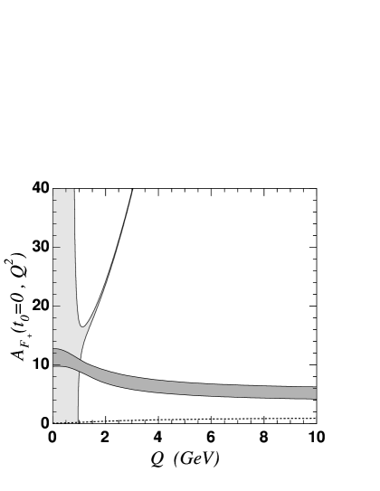
Figure 1: Bounds on the expansion coefficients for the vector form factor. The top (light) band represents the unitarity bound, and the lower (dark) band is a direct evaluation from $\tau$ decay and perturbative QCD. The perturbative contribution is shown separately as the dashed line.

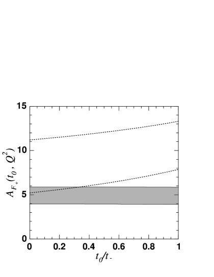
Figure 2: Bounds on $A_{F_{+}}$ in (9), as a function of $t_{0}$. The dashed lines are for the default choice of $\phi_{F_{+}}$ in (II), with $Q=0$ (top) and $Q=10\,{\rm GeV}$ (bottom). The solid band gives the ($Q$-independent) result when $\phi_{F_{+}}\equiv 1$.

Although the OPE breaks down at small $Q$, the norm in (4) remains perfectly well defined. The dark band in Fig. 1 shows the result of evaluating the integral in (4) using $\tau\to K\pi\nu$ decay data Barate:1999hj for the region $t_{+}<t<m_{\tau}^{2}$, and estimating the remaining contribution from $t>m_{\tau}^{2}$ using perturbative QCD. Uncertainties from the $\tau$ decay data are conservatively estimated by taking the maximum (minimum) value of the weight function in (4) for each bin, and multiplying by the corresponding upper (lower) bound of the $1\sigma$ interval for the $K\pi$ component of the spectral function measured in Barate:1999hj . It may be noted that for the present purpose, there is no need to resolve the underlying resonance structure of the spectral function, nor to subtract the (small) $S$-wave contribution.

The remaining perturbative contribution is estimated using $F_{+}(t)\sim 8\pi f_{\pi}f_{K}\alpha_{s}/t$ Lepage:1980fj , conservatively setting $\alpha_{s}\approx 1$, and assigning $100\%$ uncertainty to the result. The effect is $\Delta A_{F_{+}}^{2}\lesssim 2$ for all values of $Q\in(0,10\,{\rm GeV})$, and is insignificant when added in quadrature to the much larger contribution from the resonance region.

As illustrated by Fig. 2, the dependence of $A_{F_{+}}$ on $t_{0}$ is very mild. Here we again set $F_{+}(t_{0})\approx 1$; this is strictly an overestimate, and accounts for much of the $t_{0}$ variation in the figure. The norm for all schemes (II) with $0<t_{0}<t_{-}$ and $0<Q<10\,{\rm GeV}$ satisfies

$$A_{F_{+}}(t_{0},Q^{2})\lesssim 13\,.$$ (11)

More refined values for $A_{F_{+}}$ can be obtained from Figs. 1 and 2 at particular values of $t_{0}$ and $Q$.

The result from the OPE represents an upper bound for $A_{F_{+}}$. For large $Q$, the leading contributions to $A_{F_{+}}$ are ${\cal O}(Q^{0})$, coming from the regions $t\sim\Lambda_{\rm QCD}^{2}$, and $t\sim Q^{2}$ in (4).  The OPE overestimates $A_{F_{+}}$ by a factor $\sim(Q/\Lambda_{\rm QCD})^{2}$. As Fig. 1 shows, although the OPE evaluation becomes exceedingly precise, the resulting unitarity bound begins to wildly overestimate the norm of the form factor already at $Q\sim 2-3\,{\rm GeV}$.

III Scalar Form Factor Constraints

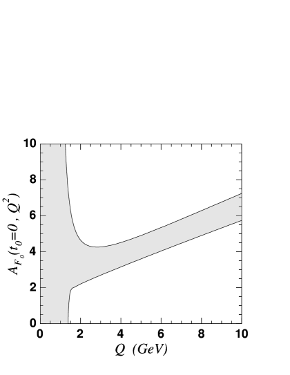
Figure 3: Bounds on the expansion coefficients for the scalar form factor.

In the scalar case, an unsubtracted dispersion relation can be written for the quantity

$$\chi_{0}(Q^{2})\equiv{\partial\over\partial q^{2}}\left[q^{2}\Pi_{0}\right]={1\over\pi}\int_{0}^{\infty}\!dt\,{t{\rm Im}\Pi_{0}(t)\over(t+Q^{2})^{2}}\,.$$ (12)

Noticing that

$${\rm Im}\Pi_{0}(t)\geq{3\over 2}{t_{+}t_{-}\over 16\pi}{[(t-t_{+})(t-t_{-})]^{1/2}\over t^{3}}|F_{0}(t)|^{2}\theta(t-t_{+})\,,$$ (13)

and defining

$$\phi_{F_{0}}(t,t_{0},Q^{2}) = \sqrt{3t_{+}t_{-}\over 32\pi}{z(t,0)\over-t}{z(t,-Q^{2})\over-Q^{2}-t}\left(z(t,t_{0})\over t_{0}-t\right)^{-1/2}$$ (14)

$$\times\left(z(t,t_{-})\over t_{-}-t\right)^{-1/4}{\sqrt{t_{+}-t}\over(t_{+}-t_{0})^{1/4}}\,,$$

yields the inequality

$$A_{F_{0}}^{2}(t_{0},Q^{2})\equiv\sum_{k}{a_{k}^{2}\over a_{0}^{2}}\leq{\chi_{0}(Q^{2})\over|\phi_{F_{0}}(t_{0},t_{0},Q^{2})F_{0}(t_{0})|^{2}}\,.$$ (15)

Again, $\chi_{0}(Q^{2})$ can be reliably calculated when $Q\gg\Lambda_{\rm QCD}$ Chetyrkin:1996sr ; Generalis:1983hb :

$$\chi_{0}(Q^{2}) = {3m_{s}^{2}\over 8\pi^{2}Q^{2}}\big{[}1+1.80\alpha_{s}+4.65\alpha_{s}^{2}+15.0\alpha_{s}^{3}+\dots\big{]}$$ (16)

$$+{1\over Q^{4}}\big{[}m_{s}\left(\langle\bar{u}u\rangle-\langle\bar{s}s\rangle\right)+\dots\big{]}+\dots\,,$$

where $m_{s}(2\,{\rm GeV})=0.087(8)\,{\rm GeV}$ Mason:2005bj , $m_{s}(\langle\bar{u}u\rangle-\langle\bar{s}s\rangle)=-0.0006(3)\,{\rm GeV}^{4}$ Narison:2002hk . The light band in Fig. 3 shows the $1\sigma$ contour obtained by adding errors from all sources linearly, as described after (II); in this case, higher-order contributions of relative size $\pm 10\times\alpha_{s}^{4}$ are included. 

The behavior of the unitarity bound with respect to $Q$ is milder than in the vector case. For large $Q$, the leading contributions to $A_{F_{0}}$ are ${\cal O}(Q^{0})$, coming from the regions $t\sim\Lambda_{\rm QCD}^{2}$ and $t\sim Q^{2}$ in (4).  Again, it should be remembered that the OPE gives an upper bound to $A_{F_{0}}$, although for this case the bound is overestimated by only a single power of $Q/\Lambda_{\rm QCD}$. While it is not possible to rigorously bound the norm of $F_{0}$ using the OPE for schemes with $Q\lesssim\Lambda_{\rm QCD}$, there is no parametric enhancement of the integral in (15) for these $Q$ values. A conservative bound on the norm for all schemes with $0<t_{0}<t_{-}$ and $0<Q<10\,{\rm GeV}$ is

$$A_{F_{0}}(t_{0},Q^{2})\lesssim 5\,.$$ (17)

In principle, this bound could be improved by extracting the $K\pi$ component of the scalar spectral function from $\tau\to K\pi\nu$.

IV Implications for $K_{\ell 3}$ and $|V_{us}|$

To implement the expansion (3) we must choose a “scheme” specified by the functional form of $\phi$, and by the values of $Q^{2}$ and $t_{0}$. Possible candidates for $\phi$ are $\phi=1$, or $\phi$ given by (II) and (14). The latter choice ensures that the norm in (4) is independent of $t_{0}$ and relates in a simple way to the spectral functions extracted from $\tau$ decay; with, say $Q^{2}=2\,{\rm GeV}^{2}$, this choice also allows comparison to OPE bounds. 

The value of $t_{0}$ can be selected according to various criteria. For example, the choice $t_{0}=t_{+}(1-\sqrt{1-t_{-}/t_{+}})$ minimizes the maximum value of $z$ throughout the semileptonic range, while $t_{0}=0$ simplifies the translation between coefficients $a_{k}$ and the derivatives of the form factor at $t=0$. Alternatively, the choice of $t_{0}$ can be used to minimize correlations between shape parameters.

When only a single form factor contributes (as in $K_{e3}$ decays), the error correlations between expansion coefficients $a_{k}(t_{0},Q^{2})$ measured in an experiment with near ideal acceptance and resolution are completely determined without a priori knowledge of the form factor shape. With $\Delta\Gamma_{i}/\Gamma_{i}\propto 1/\sqrt{\Gamma_{i}}$ where $\Gamma_{i}\sim p(t_{i})^{3}F_{+}(t_{i})^{2}$ are partial rates measured in intervals of $t$, it follows that the error matrix $U$ determined from a $\chi^{2}$ fit is: (here $p=|\mbox{\boldmath$p$\unboldmath}|$ is the pion momentum in the kaon rest frame)

$$U^{-1}_{kk^{\prime}}\equiv{1\over 2}{\partial^{2}\chi\over\partial a_{k}\partial a_{k^{\prime}}}\propto\int_{0}^{t_{-}}\!dt\,{p(t)^{3}\over\phi_{F_{+}}(t,t_{0},Q^{2})^{2}}z(t,t_{0})^{k+k^{\prime}}\,.$$ (18)

If the $K_{e3}$ data is fit to a normalization proportional to $F_{+}(0)$ and two shape parameters $a_{1}(t_{0},Q^{2})/a_{0}(t_{0},Q^{2})$ and $a_{2}(t_{0},Q^{2})/a_{0}(t_{0},Q^{2})$, the correlation between $a_{1}/a_{0}$ and $a_{2}/a_{0}$ vanishes in the ideal case for $t_{0}\approx 0.39\,t_{-}$ (with $\phi_{F_{+}}$ as in (II) and $Q^{2}=2\,\rm GeV^{2}$). 

IV.1 $F_{+}$ and $K_{e3}$

Only the vector form factor is relevant for the electron mode. From (11) and $|z|\lesssim 0.05$ [at $t_{0}=t_{+}(1-\sqrt{1-t_{-}/t_{+}})$], the quadratic term, $a_{2}z^{2}$ in (3), can affect the normalization by an amount not greater than $A_{F_{+}}|z|^{2}<0.029$. To establish a precision significantly smaller than this, $a_{2}$ must be constrained by data. The cubic term is bounded by $A_{F_{+}}|z|^{3}<0.0014$. These errors can also be robustly estimated by including higher order terms in fits to the experimental data, under the constraint (11). Extraction of other observables, such as the form factor slope and curvature at $t=0$ can be treated similarly.

The simple Taylor expansion in $t$ converges much more slowly than the $z$ expansion in (3), and it is difficult to reliably bound the errors associated with higher-order terms in fits to the truncated $t$ series. The systematic approach advocated here should remedy this situation, and make a more definitive comparison between different experiments possible. 

IV.2 $F_{0}$ and $K_{\mu 3}$

The scalar form factor can be probed in the muon mode. With enough precision, constraining the slope of this form factor could aid lattice and chiral perturbation theory estimates of $F_{+}(0)=F_{0}(0)$ by eliminating extrapolation errors Becirevic:2004ya , or by determining higher-order constants in the chiral Lagrangian Bijnens:2003uy . In a general scheme: (the prime denotes derivative with respect to $t$)

$${F_{0}^{\prime}(0)\over F_{0}(0)}\!=\!-{\phi_{F_{0}}^{\prime}(0,t_{0},Q^{2})\over\phi_{F_{0}}(0,t_{0},Q^{2})}+z^{\prime}(0,t_{0}){\dots{a_{1}\over a_{0}}+{2a_{2}\over a_{0}}z(0,t_{0})+\over 1+{a_{1}\over a_{0}}z(0,t_{0})+\dots}\,.$$ (19)

Present experiments do not strongly constrain the coefficients beyond the linear $a_{1}z$ term in (3). From (17) and $|z|\lesssim 0.05$ it is straightforward to estimate the resulting uncertainty on the slope: $\Delta[m_{\pi}^{2}F_{0}^{\prime}(0)/F_{0}(0)]\approx A_{F_{0}}\times 0.001<0.005$. This error can also be robustly estimated by including higher order terms in fits to the experimental data, under the constraint (17).

To further constrain the slope requires either more precise semileptonic data, or independent constraints on the form factor. One type of constraint appeals to symmetry principles, in particular at the Callan-Treiman point where $F_{0}(\Delta_{K\pi})={f_{K}/f_{\pi}}+\Delta_{CT}$ with a controllably small correction, $\Delta_{CT}$ Gasser:1984ux . Unfortunately, this point is too far removed from $t=0$ to have a very strong influence on the extraction of $F^{\prime}_{0}(0)/F_{0}(0)$.  As a second type of constraint, the phase of the form factor above $K\pi$ threshold can be determined from $K\pi$ scattering. Even supposing arbitrarily precise scattering data were available up to the inelastic threshold, $t_{\rm inel}=(m_{K}+3m_{\pi})^{2}$, it is easy to see that dramatic constraints are not expected in the semileptonic region. Since the additional data relates to the form factor at points along the cut in the $t$-plane, where $|z(t,t_{0})|=1$, constraints from the scattering data can be satisfied by tuning higher-order coefficients $a_{k}$ in (3), which have relatively minor impact in the semileptonic region. More quantitatively, with arbitrarily precise data, a suitable phase redefinition of the form factor (a particular choice of $\phi$) can postpone the branch point in $\phi F$ until $t_{\rm inel}$. Replacing $t_{+}$ with $t_{\rm inel}$ in (2) , we see that the maximum size of the effective expansion parameter can then be made as small as $|z|\lesssim 0.021$ throughout the semileptonic region, compared to $|z|\lesssim 0.047$ when the branch point appears at $t_{+}$. Thus while some improvement is possible by directly incorporating the experimental scattering data, more dramatic gains in precision require further dynamical inputs or assumptions Jamin:2006tj .

V Implications beyond $K_{\ell 3}$

The general parameterization (3), with constraints (11) and (17), can be used to systematically analyze the $K\to\pi\ell\nu$ data without model assumptions. This should eliminate a dominant uncertainty in the experimental determination of $|V_{us}F_{+}(0)|$, and allow for a more definitive comparison of shape observables measured by different experiments.

$K_{\ell 3}$ decays provide a unique opportunity to investigate the convergence properties of the expansion (3). Precision data can be used to directly constrain the first few coefficients, and the existence of a heavy lepton, $m_{\tau}\gg m_{K}+m_{\pi}$, makes it possible to establish bounds on the dominant vector form factor that are both more stringent and more generally applicable than those obtained from an OPE analysis. This provides a direct test of scaling arguments that apply also in the charm and bottom systems Becher:2005bg .

Acknowledgements. The author acknowledges a number of fruitful discussions with A. Glazov and R. Kessler. Thanks also to T. Becher for comments on the manuscript, and M. Davier for a useful remark concerning the details of Ref. Barate:1999hj . Fermilab is operated by Universities Research Association Inc. under contract DE-AC02-76CH03000 with the U.S. Department of Energy.

References

- (1) For a review see: E. Blucher et al., hep-ph/0512039.
- (2) T. Alexopoulos et al. [KTeV Collaboration], Phys. Rev. D 70, 092007 (2004).
- (3) A. Lai et al. [NA48 Collaboration], Phys. Lett. B 604, 1 (2004).
- (4) O. P. Yushchenko et al., Phys. Lett. B 589, 111 (2004).
- (5) F. Ambrosino et al. [KLOE Collaboration], Phys. Lett. B 636, 166 (2006).
- (6) D. Becirevic et al., Nucl. Phys. B 705, 339 (2005).
- (7) J. Bijnens and P. Talavera, Nucl. Phys. B 669, 341 (2003). For further references, see: J. Bijnens, hep-ph/0604043.
- (8) See e.g.: C. Bourrely, B. Machet and E. de Rafael, Nucl. Phys. B 189, 157 (1981), and references therein. Early applications to heavy-meson decays and related developments can be found in: C. G. Boyd, B. Grinstein and R. F. Lebed, Phys. Rev. Lett. 74, 4603 (1995); L. Lellouch, Nucl. Phys. B 479, 353 (1996); I. Caprini and M. Neubert, Phys. Lett. B 380, 376 (1996).
- (9) L. V. Ahlfors, Complex Analysis, McGraw-Hill, 1953.
- (10) T. Becher and R. J. Hill, Phys. Lett. B 633, 61 (2006).
- (11) S. G. Gorishnii, A. L. Kataev and S. A. Larin, Phys. Lett. B 259, 144 (1991). L. R. Surguladze and M. A. Samuel, Phys. Rev. Lett. 66, 560 (1991) [Erratum-ibid. 66, 2416 (1991)]. K. G. Chetyrkin, Phys. Lett. B 391, 402 (1997).
- (12) S. C. Generalis and D. J. Broadhurst, Phys. Lett. B 139, 85 (1984).
- (13) Q. Mason, H. D. Trottier, R. Horgan, C. T. H. Davies and G. P. Lepage [HPQCD Collaboration], Phys. Rev. D 73, 114501 (2006).
- (14) S. Narison, hep-ph/0202200.
- (15) R. Barate et al. [ALEPH Collaboration], Eur. Phys. J. C 11, 599 (1999).The spectral function in Fig. 9 of this reference is related to in (7) by .
- (16) G. P. Lepage and S. J. Brodsky, Phys. Rev. D 22, 2157 (1980).
- (17) K. G. Chetyrkin, Phys. Lett. B 390, 309 (1997).
- (18) R. J. Hill, Phys. Rev. D 73, 014012 (2006).
- (19) J. Gasser and H. Leutwyler, Nucl. Phys. B 250, 517 (1985).
- (20) For some recent analysis along these lines, see: M. Jamin, J. A. Oller and A. Pich, hep-ph/0605095. V. Bernard, M. Oertel, E. Passemar and J. Stern, hep-ph/0603202.
- (21) C. Bourrely and I. Caprini, Nucl. Phys. B 722, 149 (2005).