ANL-HEP-PR-06-53 CU-TP-1152 EFI-06-08 FERMILAB-PUB-06/234-T hep-ph/0607106 Light Kaluza-Klein States in Randall-Sundrum Models with Custodial $SU(2)$

Abstract

We consider Randall-Sundrum scenarios based on $SU(2)_{L}\times SU(2)_{R}$ and a discrete parity exchanging $L$ with $R$. The custodial and parity symmetries can be used to make the tree level contribution to the $T$ parameter and the anomalous couplings of the bottom quark to the $Z$ very small. We show that the resulting quantum numbers typically induce a negative $T$ parameter at one loop that, together with the positive value of the $S$ parameter, restrict considerably these models. There are nevertheless regions of parameter space that successfully reproduce the fit to electroweak precision observables with light Kaluza-Klein excitations accessible at colliders. We consider models of gauge-Higgs unification that implement the custodial and parity symmetries and find that the electroweak data singles out a very well defined region in parameter space. In this region one typically finds light gauge boson Kaluza-Klein excitations as well as light $SU(2)_{L}$ singlet, and sometimes also doublet, fermionic states, that mix with the top quark, and that may yield interesting signatures at future colliders.

1 Introduction

The LHC era that is about to start is expected to unravel the mysteries of electroweak (EW) symmetry breaking and the origin of the gauge hierarchy. Among the theories that attempt to explain the hierarchy problem, the Randall-Sundrum model [1] stands out as one of the most promising ones. The well-known little hierarchy problem becomes, however, critical in such a model. In fact, it is not just a matter of fine-tuning, but also that the EW precision data turn out to be so constraining that the masses of the Kaluza-Klein (KK) modes of bulk fields are pushed to scales that make their discovery at the LHC extremely challenging. Even though placing the fermions (together with the gauge bosons) in the bulk softens the constraints, there is still a very large contribution to the Peskin-Takeuchi [2] $T$ parameter [3]. The presence of infrared (IR) brane kinetic terms [4] can reduce the size of the oblique corrections and, if large enough, induce a spectrum of gauge KK modes accessible at colliders [5, 6]. In this paper we will consider a different alternative based on custodial symmetry. It was noticed in [7] that extending the bulk gauge symmetry to a custodially symmetric $SU(2)_{L}\times SU(2)_{R}$, also reduces the tree level contribution to the $T$ parameter to phenomenologically allowed levels for masses of the KK excitations of the gauge bosons $M_{KK}\sim 3$ TeV. At the same time, the Right-Handed (RH) quarks were included in doublets under the $SU(2)_{R}$ symmetry bringing with them $SU(2)_{R}$-symmetric partners that in the case of the RH top quark can be very light. Unfortunately, this mode mixes with the bottom quark and induces anomalous couplings to the $Z$ that again puts strong constraints on these models, pushing the KK modes beyond experimental detectability. However, it has been very recently pointed out [8] that the custodial symmetry together with a discrete $L\leftrightarrow R$ symmetry can protect the $b$ coupling to the $Z$ from anomalous corrections, therefore apparently saving the last hurdle for a realistic Randall-Sundrum model with small brane kinetic terms and observable KK modes at the LHC. In this article we show that, although the custodial and $LR$ parity symmetries are very powerful in rendering the tree level contributions to the $T$ parameter and the $Z\bar{b}_{L}b_{L}$ coupling very small, the quantum numbers we are forced upon to get such a protection – bidoublets under the $SU(2)_{L}\times SU(2)_{R}$ symmetry – typically induce sizable and negative contributions to $T$ at the loop level. Such negative contribution to the $T$ parameter, together with a positive value of the $S$ parameter greatly constraint the masses of the KK modes. A scan over parameter space shows however that there are regions where the sign of $T$ is reversed and gauge boson KK masses, $M_{KK}\sim 3$ TeV, can be compatible with experimental data. Hence, we obtain the first Randall-Sundrum model with negligible brane kinetic terms that is fully compatible with EW precision observables and has gauge boson KK masses accessible at the LHC.

The above scenarios are based on a fundamental Higgs field, and suffer from the little hierarchy problem. An alternative theory of EW symmetry breaking, that does not require any fundamental scalars, has received a lot of attention recently in the context of models with extra dimensions. These are the models of “gauge-Higgs unification” [9, 10], where the Higgs field is a pseudo-Nambu-Goldstone boson that arises as the component along the extra dimensions of gauge fields of broken symmetries. The higher dimensional gauge symmetry protects the Higgs from cut-off sensitive corrections making its potential, that arises at the quantum level, finite and therefore calculable. A very simple, yet realistic example is based on an $SO(5)\times U(1)_{X}$ bulk symmetry broken to $SO(4)\times U(1)_{X}\sim SU(2)_{L}\times SU(2)_{R}\times U(1)_{X}$ on the IR brane and to $SU(2)_{L}\times U(1)_{Y}$ on the UV brane. The Higgs field corresponds to the zero mode of the $A_{5}$ gauge boson along the broken direction $SO(5)/SO(4)$ [10]. The extended gauge symmetry makes models of gauge-Higgs unification very predictive and therefore also very constrained. In particular, a light Higgs is a generic prediction of these models. Also, the fact that Yukawa couplings are really gauge couplings reduces the freedom to play with the location of the zero modes and makes it more difficult to cancel the negative contribution to the $T$ parameter generated by the bidoublets. Interestingly, the allowed regions of parameter space typically lead to fermion states well under a TeV.

The structure of the paper is the following. In section 2 we introduce the custodially symmetric version of the RS model with a fundamental Higgs, not necessarily localized on the IR brane, and review the constraints coming from oblique parameters and the $Z\bar{b}b$ coupling. We show that, as already noted in Ref. [8], in the absence of large brane kinetic terms, in order to obtain light enough KK states, accessible at the LHC, the Left-Handed (LH) quarks are required to belong to bidoublets of $SU(2)_{L}\times SU(2)_{R}$. In section 3 we compute in detail the one-loop contributions to the $T$ parameter and show that the bidoublets induce a sizable, negative $T$ in most regions of parameter space. We then consider models of gauge-Higgs unification in section 4, and identify the regions of parameter space allowed by the EW precision measurements. In section 5 we present the most relevant features of the phenomenology of this type of models, and we conclude in section 6.

2 $SU(2)_{L}\times SU(2)_{R}$ scenarios

We consider an $SU(2)_{L}\times SU(2)_{R}\times U(1)_{X}$ gauge theory on a slice of $AdS_{5}$ with metric

$$ds^{2}=e^{-2ky}\eta_{\mu\nu}dx^{\mu}dx^{\nu}-dy^{2},$$ (1)

and fifth-dimensional coordinate $0\leq y\leq L$. The fermions are allowed to propagate in the bulk. In order to address the gauge hierarchy problem, the Higgs field has to be localized near the IR brane ($y=L$). We will analyze both the case of a Higgs exactly localized on the IR brane, as well as the case of a Higgs propagating in the bulk, as it occurs in gauge-Higgs unification scenarios.

The gauge group is broken by boundary conditions to the Standard Model (SM) on the UV brane ($y=0$). This is done with the following assignment of boundary conditions

$$W^{a}_{L\,\mu}\sim(+,+)~{},\quad B_{\mu}\sim(+,+)~{},$$ (2)

$$W^{b}_{R\,\mu}\sim(-,+)~{},\quad Z^{\prime}_{\mu}\sim(-,+)~{},$$ (3)

where $+$ ($-$) stands for Neumann (Dirichlet) boundary conditions, $a=1,2,3$, $b=1,2$ and $B_{\mu}$ and $Z^{\prime}_{\mu}$ are the following two combinations of neutral gauge bosons

$$B_{\mu}=\frac{g_{5\,X}W^{3}_{R\,\mu}+g_{5\,R}X_{\mu}}{\sqrt{g^{2}_{5\,R}+g^{2}_{5\,X}}}~{},\quad\quad\quad Z^{\prime}_{\mu}=\frac{g_{5\,R}W^{3}_{R\,\mu}-g_{5\,X}X_{\mu}}{\sqrt{g^{2}_{5\,R}+g^{2}_{5\,X}}}~{},$$ (4)

with $g_{5\,R},g_{5\,X}$ the five-dimensional coupling constants of the $SU(2)_{R}$ and $U(1)_{X}$ groups, respectively. The covariant derivative in the basis of well defined parities then reads

$$D_{\mu}=\partial_{\mu}-\mathrm{i}\left[g_{5\,L}W^{a}_{L\,\mu}T^{a}_{L}+g_{5}^{\prime}\frac{Y}{2}B_{\mu}+g_{5\,R}W^{b}_{R\,\mu}T^{b}_{R}+g_{5\,Z^{\prime}}Q_{Z}^{\prime}Z^{\prime}_{\mu}\right]~{},$$ (5)

where the hypercharge and $Z^{\prime}$ gauge couplings are

$$g_{5}^{\prime}=\frac{g_{5\,R}\,g_{5\,X}}{\sqrt{g^{2}_{5\,R}+g^{2}_{5\,X}}}~{},\quad\quad\quad g_{5\,Z^{\prime}}=\sqrt{g^{2}_{5\,R}+g^{2}_{5\,X}}~{},$$ (6)

whereas the charges are

$$\frac{Y}{2}=T^{3}_{R}+Q_{X}~{},\quad\quad\quad Q_{Z}^{\prime}=\frac{g_{5\,R}^{2}T^{3}_{R}-g_{5\,X}^{2}Q_{X}}{g_{5\,R}^{2}+g_{5\,X}^{2}}~{},$$ (7)

so that the electric charge reads

$$Q=T^{3}_{L}+T^{3}_{R}+Q_{X}~{}.$$ (8)

The modes with $(+,+)$ boundary conditions have zero modes that make the gauge bosons of the SM whereas the ones with $(-+)$ boundary conditions only have massive modes. We can now integrate out these and the KK excitations of the SM gauge bosons to obtain a four-dimensional effective theory that can be compared to experiment.

2.1 Tree-level Corrections from Gauge KK Modes

The massive gauge bosons induce tree-level corrections to the SM gauge boson masses and to their couplings to the fermions (as well as four-fermion interactions). Given that the KK scale is well above the EW breaking scale, we may treat the Higgs vacuum expectation value (vev) perturbatively and keep only the leading corrections. These can be expressed in terms of the zero-momentum gauge boson propagators for the massive KK modes obeying $(+,+)$ boundary conditions. More precisely, in terms of the coefficient of $P_{\mu\nu}=\eta_{\mu\nu}-p_{\mu}p_{\nu}/p^{2}$, with zero mode parts subtracted [5] :

$$\widetilde{G}^{++}_{p=0}(y,y^{\prime}) = \frac{1}{4k(kL)}\bigg{\{}\frac{1-e^{2kL}}{kL}+e^{2ky_{<}}(1-2ky_{<})+e^{2ky_{>}}\left[1+2k(L-y_{>})\right]\bigg{\}}~{},$$ (9)

and those obeying $(-,+)$ boundary conditions:

$$\widetilde{G}^{-+}_{p=0}(y,y^{\prime}) = -\frac{1}{2k}\left[e^{2ky_{<}}-1\right]~{}.$$ (10)

Here $p$ is the 4-dimensional momentum and $y_{<}$ ($y_{>}$) denote the smallest (largest) of $y$ and $y^{\prime}$, the fifth-dimensional coordinate.

To leading order in the corrections, the SM gauge boson masses are

$$m^{2}_{Z} = \frac{e^{2}v^{2}}{2s^{2}c^{2}}\bigg{\{}1+\frac{e^{2}}{s^{2}c^{2}}\left[\delta^{2}_{++}+\left(\frac{g_{R}^{2}}{g_{L}^{2}}c^{2}-s^{2}\right)\delta^{2}_{-+}\right]+\cdots\bigg{\}}~{},$$ (11)

$$m^{2}_{W} = \frac{e^{2}v^{2}}{2s^{2}}\bigg{\{}1+\frac{e^{2}}{s^{2}}\left[\delta^{2}_{++}+\frac{g_{R}^{2}}{g_{L}^{2}}\delta^{2}_{-+}\right]+\cdots\bigg{\}}~{},$$ (12)

where $v=174~{}\rm{GeV}$ is the SM Higgs vev, four-dimensional couplings are defined in terms of the five-dimensional ones as $g_{L}=g_{5\,L}/\sqrt{L}$ (similarly for the rest), and we have defined as it is customary

$$e=\frac{g^{\prime}\,g_{L}}{\sqrt{g_{L}^{2}+g^{\prime\,2}}}~{},\quad s=\frac{e}{g_{L}}~{},\quad c=\sqrt{1-s^{2}}~{}.$$ (13)

The corrections from exchange of the towers of the $W^{a}_{L}$ and hypercharge $B$ gauge bosons are contained in

$$\delta^{2}_{++} = \frac{Lv^{2}}{2}\int^{L}_{0}\!dydy^{\prime}e^{-2ky}f_{H}(y)^{2}\widetilde{G}^{++}_{p=0}(y,y^{\prime})e^{-2ky^{\prime}}f_{H}(y^{\prime})^{2}~{}.$$ (14)

The function $f_{H}(y)$ is the Higgs profile which is kept arbitrary for the time being. The contributions from the $W^{b}_{R}$ and the neutral $Z^{\prime}$ towers are encoded in $\delta^{2}_{-+}$, which is defined as in Eq. (14), but in terms of the massive propagator given in Eq. (10).

The corrections to the couplings of the SM gauge bosons to the fermion currents depend on the fermion zero-mode wavefunctions. The couplings to the $Z$ take the form

$$\frac{e}{sc}Z_{\mu}\sum_{\psi}\bigg{\{}\bar{\psi}^{(0,r)}\gamma^{\mu}\left(T^{3}_{L}-s^{2}Q\right)\psi^{(0,r^{\prime})}\left[\delta^{rr^{\prime}}+\frac{e^{2}}{s^{2}c^{2}}G^{rr^{\prime}}_{++}\right]$$

$$\mbox{}-\frac{e^{2}}{s^{2}c^{2}}\bar{\psi}^{(0,r)}\gamma^{\mu}\left(\frac{g_{R}^{2}}{g_{L}^{2}}c^{2}T^{3}_{R}+s^{2}T^{3}_{L}-s^{2}Q\right)\psi^{(0,r^{\prime})}G^{rr^{\prime}}_{-+}\bigg{\}}~{},$$ (15)

where the sum runs over all chiral fermions. Here,

$$G^{rr^{\prime}}_{++} = \frac{v^{2}}{2}\int^{L}_{0}\!dydy^{\prime}\left[f^{0}_{\psi^{r}}(y)\right]^{*}f^{0}_{\psi^{r^{\prime}}}(y)\widetilde{G}^{++}_{p=0}(y,y^{\prime})e^{-2ky^{\prime}}f_{H}(y^{\prime})^{2}~{},$$ (16)

where $\widetilde{G}^{++}_{p=0}(y,y^{\prime})$ was defined in Eq. (9), and $f^{0}_{\psi^{r}}(y)$ is the zero-mode wavefunction for the fermion $\psi^{r}$, $r$ being a flavor index. $G^{rr^{\prime}}_{-+}$ is defined analogously in terms of the propagator of Eq. (10).

Similarly, the charged currents read

$$\frac{e}{\sqrt{2}s}W^{+}_{\mu}\sum_{\psi}\bigg{\{}\bar{\psi}^{(0,r)}\gamma^{\mu}T^{+}_{L}\psi^{(0,r^{\prime})}\left[\delta^{rr^{\prime}}+\frac{e^{2}}{s^{2}}G^{rr^{\prime}}_{++}\right]+\frac{g_{R}^{2}}{g_{L}^{2}}\frac{e^{2}}{s^{2}}\bar{\psi}^{(0,r)}\gamma^{\mu}T^{+}_{R}\psi^{(0,r^{\prime})}G^{rr^{\prime}}_{-+}\bigg{\}}+{\rm h.c.}$$ (17)

where $T_{L,R}^{+}=T_{L,R}^{1}+iT_{L,R}^{2}$ and the sum runs over all chiral fermions.

In the general case, the previous corrections are flavor-dependent and would set very stringent bounds on the masses of the KK modes. However, it is well known that these effects can be controlled effectively in RS scenarios by localizing the fermions of the first two generations closer to the UV brane than to the IR brane [11]. In fact, in this region of parameter space the quantities $G^{rr^{\prime}}_{++}$ and $G^{rr^{\prime}}_{-+}$ become essentially independent of the fermion profile, thus leading to universal effects that can be recast in the form of oblique corrections. Furthermore, in this same region it becomes possible to generate the fermion mass hierarchies entirely from the overlaps between the Higgs and fermion wavefunctions. Therefore, we concentrate on this scenario, which allows us to parametrize the corrections to the Z-pole observables measured at LEP and SLD together with the mass of the $W$ measured at the Tevatron and LEP2 in terms of the Peskin-Takeuchi $S$, $T$ and $U$ parameters [2].

For the first two quark and lepton generations as well as the third generation leptons, the general couplings to the $Z$ and $W$ given in Eqs. (2.1) and (17) reduce to

$$\frac{e}{sc}Z_{\mu}\left[\bar{\psi}^{(0,r)}\gamma^{\mu}\left(T^{3}_{L}-s^{2}Q\right)\psi^{(0,r)}\right]\left(1+\frac{e^{2}}{s^{2}c^{2}}\,G^{f}_{++}\right)~{},$$ (18)

and

$$\frac{e}{\sqrt{2}s}W_{\mu}^{+}\left[\bar{\psi}^{(0,r)}\gamma^{\mu}T^{+}_{L}\psi^{(0,r)}\right]\left(1+\frac{e^{2}}{s^{2}}\,G^{f}_{++}\right)~{},$$ (19)

where we denote by $G^{f}_{++}$ the common value of Eq. (16) for the fermions with $c_{i}>1/2$, and used the fact that the corrections proportional to $G^{rr^{\prime}}_{-+}$ in Eqs. (2.1) and (17) become negligible for such values of $c_{i}$. Since these shifts are universal they may be absorbed by a rescaling of the gauge boson fields which allows to describe these effects in terms of the oblique parameters $S$, $T$ and $U$. In fact, to describe the Z-pole observables it is possible to take into account the most important non-oblique corrections, coming from KK exchange contributions to the Fermi constant, $G_{F}$, by using the effective parameters of [4]

$$S_{\rm eff} = 32\pi G^{f}_{++}~{},$$

$$T_{\rm eff} = \frac{8\pi}{c^{2}}G^{f}_{++}-\frac{4\pi}{c^{2}}\left[\delta_{++}^{2}-\delta_{-+}^{2}\right]+\frac{2\pi v^{2}}{s^{2}}G^{\mu\mu}_{++}~{},$$ (20)

$$U_{\rm eff} = -8\pi v^{2}G^{\mu\mu}_{++}~{}.$$

In the above,

$$G^{\mu\mu}_{++} = \frac{1}{L}\int^{L}_{0}\!dydy^{\prime}|f_{\mu}^{(0)}(y)|^{2}\widetilde{G}^{++}_{p=0}(y,y^{\prime})|f_{\mu}^{(0)}(y^{\prime})|^{2}~{}$$ (21)

represents the contribution to muon decay from the exchange of the KK towers of the $SU(2)_{L}$ gauge bosons, with $f_{\mu}^{(0)}(y)$ the wave function of the muon zero mode. The Higgs vev is $v=174~{}{\rm GeV}$. In general, there are also terms proportional to $G^{f}_{-+}$ and $G^{\mu\mu}_{-+}$, that have not been included in Eq. (20) since they become negligibly small when the leptons and the first two quark generations are localized close to the UV brane. Furthermore, as is apparent from Eq. (2.1), these corrections depend on the relative values of $T^{3}_{R}$ and $T^{3}_{L}$. Hence, whenever these corrections become important, non-universal fermion-gauge-boson couplings are induced, even when all fermions are localized identically. Thus, although localizing the leptons and first two quark generations near the conformal point can be interesting due to the possibility of a small coupling to the lightest gauge boson KK modes, a determination of the bounds requires a global fit to the EW observables and will be presented elsewhere [12]. In this paper we will concentrate on a region of parameter space where an analysis based on the effective parameters $S$, $T$ and $U$ is sufficient. Consequently, we have not included such terms in Eqs. (20).

We see in the expression for $T$ in Eq. (20) the custodial symmetry mechanism at work: the largest contribution coming from the fermion-independent terms parametrized by $\delta^{2}_{++}$ of Eq. (14) is partially canceled by the corresponding contribution associated with the $Z^{\prime}$ gauge boson, parametrized by $\delta^{2}_{-+}$. The cancellation is not perfect due to the breaking of the custodial symmetry induced by the choice of boundary conditions. Thus, one finds that the tree-level contribution to the $T$ parameter is not identically zero, although, in practice, it is quite small. We have evaluated the effects due to the KK-tower contributions to $G_{F}$, which are also rather small in the region we are considering, so that $U_{\rm eff}$ is very small. Thus, in Eq. (20) it is the $S$ parameter that receives the largest contributions, and generically leads to strong bounds on the present class of scenarios. It is important to note that in the models under study, in which the light fermions are localized far from the IR brane, the $S$ parameter is always positive. In section 3 we will show that the residual loop-level contributions to the $T$ parameter are also quite relevant.

The third quark generation doublet needs to be localized closer to the IR brane in order to generate the large top mass. As a result, one should introduce an additional parameter that allows to describe the difference in the corrections to the coupling of the bottom quark with respect to the light quarks. The accurate measurement of $R_{b}$, the ratio of the width of the Z-boson decay into bottom-quarks and the total hadronic width, puts strong constraints on this difference. Since the LH bottom coupling to the Z is roughly five times larger than the RH one, this mostly constrains the former. The RH coupling, in turn, is mainly constrained by the measurement of the forward-backward and left-right bottom quark asymmetries measured at the LEP and SLD colliders. However, these constraints are much weaker than those affecting the LH coupling [13, 14]. Moreover, since the experimental value of $R_{b}$ is approximately one standard deviation larger than the value predicted by the SM, positive and negative corrections on this coupling are not equally constrained. Approximately, at the 2-$\sigma$ level, assuming no large correction to the RH bottom coupling, the constraint on the correction to the LH bottom coupling to the $Z$ reads [14],

$$-2\times 10^{-3}\begin{array}[]{c}\,\sim\vspace{-21pt}\\ <\end{array}\frac{\delta g_{b\,L}}{g_{b\,L}}\begin{array}[]{c}\,\sim\vspace{-21pt}\\ <\end{array}6\times 10^{-3}.$$ (22)

Since the LH bottom couples to the $SU(2)_{R}$ and/or $U(1)_{X}$ gauge bosons, the shift in its coupling to the $Z$, given in Eq. (2.1), receives a contribution from the terms proportional to $G^{b_{L}}_{-+}$. After rescaling the $Z$ wave function so that its couplings to the first two generations do not present anomalous shifts, the value of the anomalous LH bottom quark coupling to the $Z$ is given by

$$\frac{\delta g_{b\,L}}{g_{b\,L}}=\frac{e^{2}}{s^{2}c^{2}}\left[G^{b_{L}}_{++}-\frac{c^{2}T^{3}_{R}g_{R}^{2}/g_{L}^{2}+s^{2}T^{3}_{L}-s^{2}Q}{T^{3}_{L}-s^{2}Q}G^{b_{L}}_{-+}-G^{f}_{++}\right]~{},$$ (23)

where $T^{3}_{L}=-1/2$ and $Q=-1/3$ are the $SU(2)_{L}$ isospin and charge quantum numbers of the LH bottom quark, respectively. $T^{3}_{R}$ is the bottom quark $SU(2)_{R}$ isospin, which is determined by the embedding into the 5D gauge group representation.

For the case of $T_{R}^{3}=0$, negative corrections to $\delta g_{b\,L}/g_{b\,L}$ are generated, that become larger in absolute value as the LH bottom is localized closer to the infrared brane. Indeed, for $T^{3}_{R}(b_{L})=0$, Eq. (23) gives

$$\frac{\delta g_{b\,L}}{g_{b\,L}}(T^{3}_{R}=0)=\frac{e^{2}}{s^{2}c^{2}}\left[G^{b_{L}}_{++}-s^{2}\frac{T^{3}_{L}-Q}{T^{3}_{L}-s^{2}Q}G^{b_{L}}_{-+}-G^{f}_{++}\right]\approx\frac{e^{2}}{s^{2}c^{2}}\left[G^{b_{L}}_{++}-0.09G^{b_{L}}_{-+}-G^{f}_{++}\right]~{}.$$ (24)

These corrections are depicted by the curve labeled by “gauge” in Fig. 1, which we will explain in more detail below, and become small as we separate $b_{L}$ (and $t_{L}$) from the IR brane, in which case the coupling of the bottom and the light fermions to the $Z$ become similar. Note however that $t_{L}$ cannot be too far from the IR brane, since this would lead to an unacceptably small top quark Yukawa coupling.

We can also see how, when the LH bottom acquires a non-vanishing value of $T^{3}_{R}$, the $SU(2)_{R}$ custodial symmetry can protect the bottom coupling to the $Z$ [8]. If we set $T^{3}_{L}=T^{3}_{R}$ for $b_{L}$, together with $g_{R}=g_{L}$, the anomalous coupling greatly simplifies

$$\frac{\delta g_{b\,L}}{g_{b\,L}}(T^{3}_{R}=T^{3}_{L},g_{R}=g_{L})=\frac{e^{2}}{s^{2}c^{2}}\left[G^{b_{L}}_{++}-G^{b_{L}}_{-+}-G^{f}_{++}\right]~{},$$ (25)

and the contributions from $G^{b_{L}}_{++}$ and $G^{b_{L}}_{-+}$ tend to cancel as a result of the custodial symmetry and the quantum numbers of the bottom. As was the case for the $T$ parameter, the breaking due to the boundary conditions makes the cancellation imperfect. Notice that the degree of cancellation depends on both the bottom localization and the Higgs profile. Furthermore, since $G^{b_{L}}_{++}$ and $G^{b_{L}}_{-+}$ are different even when the bottom and Higgs fields are exactly localized on the IR brane, a residual effect still remains in this limit. In fact, one finds that the difference $G^{b_{L}}_{++}-G^{b_{L}}_{-+}$ increases slightly as the LH bottom comes closer to the IR brane.

Since $\delta g_{b\,L}$ measures the deviation of the bottom coupling to the $Z$ relative to the couplings of the first two generations, Eq. (25) receives an extra contribution from $G^{f}_{++}$. In particular, for an appropriate localization of the fermion fields, it is possible for the terms in Eq. (25) to cancel exactly, but we do not explore such a possibility here. Thus, although the anomalous $Z\bar{b}_{L}b_{L}$ coupling is small, it is not necessarily irrelevant.

2.2 Tree-level Corrections from Fermion KK Modes

In addition to the corrections due to the presence of massive spin-1 fields given in the previous section there are extra tree-level contributions to the couplings of the fermions to the SM gauge fields. These arise from integrating out the fermion KK modes that mix with the fermion zero-modes through the Higgs vev. Given that we are taking the first two generations to be localized away from the Higgs field, for the light quarks and leptons these mixing effects are exponentially suppressed due to the associated zero-mode wavefunction. However, for the third generation such effects can be important, as pointed out in [15].

As we will see, in the models of Ref. [7] this constraint by itself is strong enough to put the higher dimensional physics beyond the reach of the LHC. We conclude that a mechanism that suppresses the anomalous $Z\bar{b}_{L}b_{L}$ coupling as outlined at the end of the previous section seems to be an essential ingredient for these models to be viable.

Thus, we start by studying the class of models with custodial $SU(2)$, where the SM LH top and bottom arise from 5D $SU(2)_{R}$ singlets and the RH top arises from an $SU(2)_{R}$ doublet:

$$\begin{array}[]{rclcrcl}q_{L}&=&\begin{pmatrix}q^{t}_{L}(+,+)\\ q^{b}_{L}(+,+)\end{pmatrix}~{},&&Q_{R}&=&\begin{pmatrix}t_{R}(+,+)\\ b^{\prime}_{R}(-,+)\end{pmatrix}~{},\end{array}$$ (27)

where, under $SU(2)_{L}\times SU(2)_{R}$, $q\sim(2,1)$ and $Q\sim(1,2)$. We also indicated the boundary conditions by assigning parities at the UV and IR branes, respectively. The choice of parities is determined by the requirement that the low-energy theory should have a LH doublet and a RH top, and by the requirement that $SU(2)_{R}$ be preserved on the IR brane. We exhibit only the parities for the chiralities containing zero modes. The parity assignments for the opposite chiralities can be simply read from these.

The important point is that reproducing the top mass requires the localization of the zero mode in $Q$ near the IR brane. (As we mentioned in the previous section and will make explicit below, the LH doublet $q_{L}$ cannot be taken too close to the IR brane due to large corrections to the anomalous $b$ couplings.) This in turn implies that the lightest mode of $b^{\prime}_{R}$, a state with the quantum numbers of the RH bottom, becomes rather light. Its tree-level mixing with the LH bottom induces large anomalous couplings of the latter to the $Z$ gauge boson.

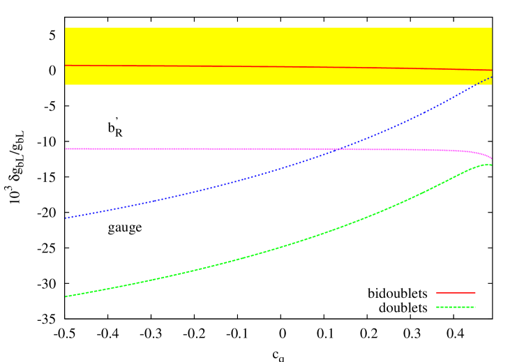
Figure 1: Contribution to $\delta g_{b\,L}/g_{b\,L}$ from Eq. (24), labeled by “gauge”, the contribution due mixing with the lightest modes of $b^{\prime}_{R}$, and the sum of the two, for models based on $SU(2)_{R}$ doublets and for $\tilde{k}=ke^{-kL}=1.5$ TeV. The solid line gives $\delta g_{b\,L}/g_{b\,L}$ from Eq. (23) for models based on bidoublets of $SU(2)_{L}\times SU(2)_{R}$. It is assumed that the Higgs is localized on the IR brane. The band is the current $2\sigma$ bound.

In Fig. 1 we plot the minimum obtainable $\delta g_{b\,L}/g_{b\,L}$ as a function of $c_{q}$, the localization parameter of the $SU(2)_{L}$ doublet, assuming the Higgs is exactly localized on the IR brane. We include the contribution due to exchange of KK gauge bosons in the case that the LH bottom is a singlet of $SU(2)_{R}$ and $g_{L}=g_{R}$, given by Eq. (24), as well as the contribution due to the mixing with the lightest $b^{\prime}_{R}$ states. The gauge contribution depends only on $c_{q}$ and the KK scale $\tilde{k}=k\,e^{-kL}$. The contribution due to mixing depends on $c_{Q}$, the localization parameter for $t_{R}$, and only very slightly on $c_{q}$. In fact, since the top mass is given in terms of the zero-mode wavefunctions by

$$m_{\rm top} = \lambda_{4}\,f_{q^{(0)}_{L}}(L)f_{t^{(0)}_{R}}(L)\,v~{},$$ (28)

where $\lambda_{4}=\lambda_{5}/L$ and $\lambda_{5}$ is the 5D top Yukawa coupling, we can express the mixing between $b^{(0)}_{L}$ and $b^{\prime(1)}_{R}$ as

$$\frac{\lambda_{4}v^{2}}{m^{2}_{b^{\prime(1)}_{R}}}f_{q^{(0)}_{L}}(L)f_{b^{\prime(1)}_{R}}(L) = \frac{m_{\rm top}v}{m^{2}_{b^{\prime(1)}_{R}}}\frac{f_{b^{\prime(1)}_{R}}(L)}{f_{t^{(0)}_{R}}(L)}~{},$$ (29)

which depends only on $c_{Q}$. The $c_{Q}$ dependence enters both through the wavefunctions and the mass of the lightest $b^{\prime}_{R}$ state. The absolute value of this function reaches a minimum for $c_{Q}\approx 0$.

The curve marked as $b^{\prime}_{R}$ in Fig. 1 corresponds to the choice of $c_{Q}$ that minimizes the contribution to $\delta g_{b\,L}/g_{b\,L}$, and is almost constant as a function of $c_{q}$ (the slight $c_{q}$ dependence is due to the higher KK modes). We took $\tilde{k}=1.5~{}{\rm TeV}$, that corresponds to gauge boson masses of approximately $3.75~{}{\rm TeV}$. We thus see that $\delta g_{b\,L}/g_{b\,L}$ gives a rather model independent bound on scenarios where the RH top arises from a 5D $SU(2)_{R}$ doublet, and that the bounds are rather severe, most likely putting the gauge boson KK sates beyond the reach of upcoming collider experiments. For example, even for $c_{Q}\approx 0.5$, the constraint Eq. (22) leads to $\tilde{k}\begin{array}[]{c}\sim\vspace{-21pt}\\ >\end{array}3.5~{}{\rm TeV}$, or gauge boson KK masses starting at $8.75~{}{\rm TeV}$.

In Fig. 1, we also plot $\delta g_{b\,L}/g_{b\,L}$ in models where the SM doublets arise from 5D $SU(2)_{L}\times SU(2)_{R}$ bidoublets, for which the condition $T^{3}_{R}=T^{3}_{L}$ can be fulfilled for $b_{L}$. In this case there are either no states with the quantum numbers of the LH bottom in the multiplets that couple through the top Yukawa coupling, or they come in pairs whose effects cancel against each other (due to the symmetry exchanging $L$ with $R$). There can be states that mix with the LH bottom and give a non-vanishing contribution to $\delta g_{b\,L}/g_{b\,L}$, coming from the multiplet that gives rise to the RH bottom. However, these contributions can be easily suppressed through the bottom quark Yukawa coupling. Therefore, we only plot the contribution due to the exchange of gauge KK states, as given in Eq. (25). The anomalous couplings are easily within the experimental limits, which gives a strong motivation for including the mechanism of Ref. [8] to suppress contributions to $\delta g_{b\,L}/g_{b\,L}$. In the next sections we concentrate on further constraints on scenarios with $SU(2)_{L}\times SU(2)_{R}$ bidoublets.

3 $SU(2)_{L}\times SU(2)_{R}$ bidoublets and the $T$ parameter

The custodial $SU(2)$ symmetry, which is broken only by boundary conditions, ensures that the contribution to the T parameter due to fermion loops is finite. Nevertheless, the finite contributions involving the KK modes of the top quark impose significant constraints. In fact, we will see that making the top-bottom doublet part of a bidoublet of $SU(2)_{L}\times SU(2)_{R}$ implies a rather definite prediction for the 1-loop contributions to the T parameter. We concentrate here on the top sector since it gives the largest effects. Other one-loop contributions to T, due to gauge bosons and light fermions, are much smaller [7].

The cancellation of the contributions to $\delta g_{b\,L}/g_{b\,L}$ advocated in [8] requires that the LH bottom be part of a $SU(2)_{L}\times SU(2)_{R}$ bidoublet, with $T^{3}_{L}=T^{3}_{R}$, i.e. $T^{3}_{L}+T^{3}_{R}=-1$, which implies from Eq. (8) that the bidoublet $U(1)_{X}$ charge is fixed to $X=2/3$. Therefore, in addition to the top partner, the LH bottom is accompanied by a charge $2/3$ field, $\chi^{d}$, and a charge $5/3$ field, $\chi^{u}$. Writing the Higgs field as a bidoublet of $SU(2)_{L}\times SU(2)_{R}$, we see that to write a top Yukawa coupling, the top $SU(2)_{L}$ singlet must arise either from an $SU(2)_{R}$ singlet or an $SU(2)_{R}$ triplet, with charge $X=2/3$ [the bottom $SU(2)_{L}$ singlet then must come from an $SU(2)_{R}$ triplet with charge $X=2/3$]. In the latter case, the $P_{LR}$ parity that ensures the cancellation of $\delta g_{b\,L}/g_{b\,L}$ requires an additional $SU(2)_{L}$ triplet, with couplings related to those of the $SU(2)_{R}$ triplet. Thus, we have the following possible assignments:

$$\begin{array}[]{rclrcl}Q_{L}&=&\begin{pmatrix}\chi^{u}_{L}(-,+)&q^{t}_{L}(+,+)\\ \chi^{d}_{L}(-,+)&q^{b}_{L}(+,+)\end{pmatrix}~{},&&t_{R}(+,+)\end{array}~{},$$ (31)

or

$$\begin{array}[]{rclrclrcl}Q_{L}&=&\begin{pmatrix}\chi^{u}_{L}(-,+)&q^{t}_{L}(+,+)\\ \chi^{d}_{L}(-,+)&q^{b}_{L}(+,+)\end{pmatrix}~{},&&T_{1R}=\begin{pmatrix}\psi^{\prime}_{R}(-,+)\\ t^{\prime}_{R}(-,+)\\ b^{\prime}_{R}(-,+)\end{pmatrix}~{},&&T_{2R}=\begin{pmatrix}\psi^{\prime\prime}_{R}(-,+)\\ t_{R}(+,+)\\ b^{\prime\prime}_{R}(-,+)\end{pmatrix}\end{array}~{},$$ (33)

where, in the bidoublets, $SU(2)_{L}$ acts vertically and $SU(2)_{R}$ acts horizontally. $T_{1}$ and $T_{2}$ transform as $(3,1)$ and $(1,3)$, respectively, under $SU(2)_{L}\times SU(2)_{R}$. In Eq. (33), the parity assignments on $Q$ and $T_{2}$ are determined by the requirement that $SU(2)_{R}$ be preserved on the IR brane, together with the zero-mode spectrum. The parity of the state $b^{\prime}$ in $T_{1}$ is chosen to be identical to that of $b^{\prime\prime}$ in $T_{2}$ to avoid large contributions to $\delta g_{b\,L}/g_{b\,L}$ from mixing of the bottom with light bottom-like states.

We are interested in the contributions to the $T$ parameter arising from 1-loop diagrams involving the KK modes in the above cases. We concentrate on the assignments shown in Eq. (31), but at the end of the section we comment on the results in the case that the top quark arises from the multiplets in Eq. (33). There are also contributions due to the remaining multiplets needed to embed the SM, but these can be easily suppressed either by taking moderately small 5D Yukawa couplings in those sectors or by choosing their localization parameters such that the overlap of their zero-mode with the Higgs is exponentially suppressed. The latter occurs when the light fermion modes are localized close to the UV brane, as we have assumed in this work. In the top sector, however, accommodating the top mass imposes strong constraints on such contributions.

Since the sums over KK mode loops are finite due to the nonlocal breaking of the custodial $SU(2)$ symmetry, it is possible to compute $T$ by including only the lowest lying states. We compute it by numerically diagonalizing the mass matrix of KK modes, including the mixings induced by the Higgs vev, and calculating the self-energies for $W^{1}_{\mu}$ and $W^{3}_{\mu}$, via [16]

$$T = \frac{N_{c}}{16\pi s^{2}c^{2}m^{2}_{Z}}\times$$

$$\left\{\sum_{\alpha}\sum_{i}\left(V^{L}_{\alpha i}V^{L*}_{\alpha i}+V^{R}_{\alpha i}V^{R*}_{\alpha i}\right)\theta_{+}({\cal M}^{\alpha\alpha}_{u},{\cal M}^{ii})+2\,{\rm Re}\left(V^{L}_{\alpha i}V^{R\ast}_{\alpha i}\right)\theta_{-}({\cal M}^{\alpha\alpha}_{u},{\cal M}^{ii})\right.$$

$$\left.\hskip 14.22636pt\mbox{}-\sum_{\alpha}\sum^{\alpha-1}_{\beta}\left(U^{L}_{\alpha\beta}U^{L*}_{\alpha\beta}+U^{R}_{\alpha\beta}U^{R*}_{\alpha\beta}\right)\theta_{+}({\cal M}^{\alpha\alpha}_{u},{\cal M}^{\beta\beta}_{u})+2\,{\rm Re}\left(U^{L}_{\alpha\beta}U^{R\ast}_{\alpha\beta}\right)\theta_{-}({\cal M}^{\alpha\alpha}_{u},{\cal M}^{\beta\beta}_{u})\right\}~{},$$

where $N_{c}=3$ is the number of colors and

$$\theta_{+}(y_{1},y_{2}) = y^{2}_{1}+y^{2}_{2}-\frac{2y^{2}_{1}y^{2}_{2}}{y^{2}_{1}-y^{2}_{2}}\ln\frac{y^{2}_{1}}{y^{2}_{2}}~{},$$ (35)

$$\theta_{-}(y_{1},y_{2}) = 2y_{1}y_{2}\left(\frac{2y^{2}_{1}y^{2}_{2}}{y^{2}_{1}-y^{2}_{2}}\ln\frac{y^{2}_{1}}{y^{2}_{2}}-2\right)~{}.$$ (36)

${\cal M}_{u}$ is the diagonal matrix of charge $2/3$ states ($q^{t}$, $\chi^{d}$ and $t$), and ${\cal M}$ contains the (diagonal) masses for the remaining states that do not mix among themselves ($q^{b}$ and $\chi^{u}$). $V^{L}$ ($V^{R}$) is the matrix of couplings of LH (RH) fermion fields to $W^{1}_{\mu}$ in the mass eigenstate basis, and $U^{L}$ ($U^{R}$) is the corresponding matrix of couplings of the charge $2/3$ states to $W^{3}_{\mu}$. The matrices $U^{L,R}$ are hermitian and satisfy the relations

$$(U^{L,R})^{2} = V^{L,R}V^{L,R\dagger}~{},$$

$$U^{L}{\cal M}_{u}U^{R} = V^{L}{\cal M}V^{R\dagger}~{},$$ (37)

$${\cal M} = V^{L\dagger}{\cal M}_{u}V^{R}~{},$$

which can be used to show that the UV divergences associated with the 4D momentum integration cancel in the expression for $T$.

To obtain the contribution to the $T$ parameter due to the new physics, we need to subtract the SM model top quark contribution

$$T_{\rm top} = \frac{N_{c}m^{2}_{\rm top}}{16\pi s^{2}c^{2}m^{2}_{Z}}~{},$$ (38)

where $m_{\rm top}$ is the would-be zero-mode mass, obtained after diagonalization of the mass matrix. We have checked that the result converges fast with the number of KK modes.

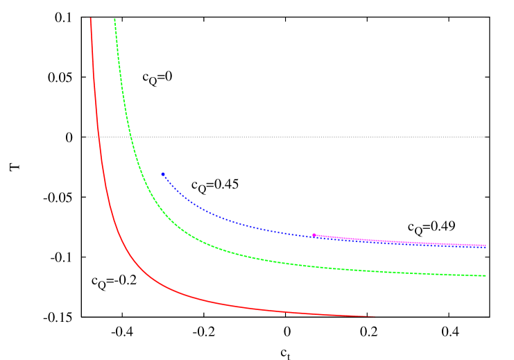
Figure 2: Contribution to the $T$ parameter involving the KK modes of Eq. (31), which couple to the Higgs through the top Yukawa coupling. We use $\tilde{k}=1.5~{}{\rm TeV}$ and $m_{\rm top}=167~{}{\rm GeV}$. The dots indicate the point beyond which the theory is strongly coupled at the scale of the first KK mode. It is assumed that the Higgs field is exactly localized on the IR brane.

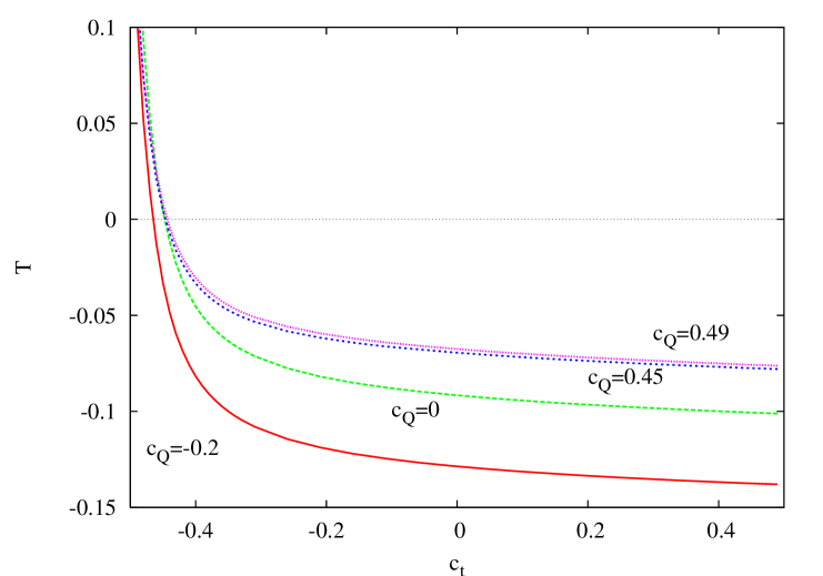
Figure 3: Contribution to the $T$ parameter involving the KK modes of Eq. (31), which couple to the Higgs through the top Yukawa coupling. We use $\tilde{k}=1.5~{}{\rm TeV}$ and $m_{\rm top}=167~{}{\rm GeV}$. It is assumed that the Higgs field has the profile of gauge-Higgs unification models, Eq. (51).

In Fig. 2 we show the $T$ parameter arising from the multiplets in Eq. (31), with the top quark contribution subtracted, as a function of $c_{t}$ and for several values of $c_{Q}$, the localization parameters of the singlet and bidoublet, respectively. It is assumed that the Higgs is localized on the IR brane. Fig. 3 shows the case where the Higgs is “maximally” delocalized [17], as would be the case in scenarios of gauge-Higgs unification (see section 4 below). There is also a contribution to $T$ coming from the gauge sector, as given in Eq. (20), which is not included in Figs. 2 or 3. It is independent of $c_{Q}$ and $c_{t}$, and is subdominant.

The figures exhibit the following features:

• $T$ becomes more negative as $c_{Q}$ decreases, which localizes the bidoublet zero-modes near the IR brane.

• As $c_{t}$ increases, which localizes $t_{R}$ near the IR brane, $T$ becomes negative.

• If we separate $t_{R}$ sufficiently from the IR brane, $T$ can become positive. However, in doing so one is forced to increase the 5D top Yukawa coupling to reproduce the top mass, eventually entering the strong coupling regime, i.e. the one-loop corrections are of the same order as the tree-level coupling. We have cut the curves when the theory is strongly coupled at the scale of the first KK mode. Thus, depending on the localization of the bidoublet, $c_{Q}$, $T$ may never reach positive values.

In fact, the negative contribution to the $T$ parameter is a direct consequence of the embedding of the SM $SU(2)_{L}$ doublets into bidoublets of $SU(2)_{L}\times SU(2)_{R}$. To clarify this point we derive approximate expressions in the case where $t$ is a singlet of $SU(2)_{R}$, as in Eq. (31). Given that the mixing masses are small compared to the scale of KK masses, it is justified to treat them perturbatively. Also, since the KK sums are convergent, we may keep only the first KK modes of the bidoublet and singlet. For clarity we consider separately the case with only the vector-like bidoublet KK modes, and the case with only the vector-like singlet KK modes included. The general (and more complicated) case can be understood from these simplified results.

Let us first consider the case that includes, in addition to the SM top and bottom, a single vector-like $SU(2)_{L}\times SU(2)_{R}$ bidoublet (in the scenarios at hand, the first KK excitations of the 5D bidoublet fields). We allow for the KK mass of the $\chi$’s to be different from the mass of the $q$’s, since they obey different boundary conditions. However, since we are treating the EW breaking vev perturbatively, we use common KK masses $M_{\chi}$ and $M_{q}$ for their upper and lower $SU(2)_{L}$ components. There are also EW breaking masses that mix the (zero-mode) singlet $t$ with the bidoublet components $q^{t}$ and $\chi^{d}$. These mixing masses, which we call $m_{q^{t},t}$ and $m_{\chi^{d},t}$ respectively, depend on the integral over the extra dimension of the Higgs zero-mode profile and the fermion wavefunctions (for the zero-mode of $t$ and the first KK modes of $q^{t}$ or $\chi^{d}$). With this notation, the lowest order contribution to the $T$ parameter takes the form

$$\Delta T=T_{\rm top}\frac{m^{2}_{\chi^{d},t}}{M^{2}_{q}}\left[-F_{1}\left(\frac{M^{2}_{q}}{M^{2}_{\chi}},\frac{m^{2}_{q^{t},t}}{m^{2}_{\chi^{d},t}},\frac{M^{2}_{\chi}}{m^{2}_{\rm top}}\right)+\frac{m^{2}_{\chi^{d},t}}{m^{2}_{\rm top}}F_{2}\left(\frac{M^{2}_{q}}{M^{2}_{\chi}},\frac{m^{2}_{q^{t},t}}{m^{2}_{\chi^{d},t}}\right)\right]~{},$$ (39)

where $T_{\rm top}$ is the SM contribution due to the top quark given in Eq. (38), and

$$F_{1}(r_{m},r_{\lambda},r_{\rm top}) = 2\left[\left(r_{m}-r_{\lambda}\right)\left(2\ln r_{\rm top}-3\right)-2r_{\lambda}\ln r_{m}\right]~{},$$ (40)

$$F_{2}(r_{m},r_{\lambda}) = \frac{4}{3(r_{m}-1)^{3}}\left\{-3r_{m}r_{\lambda}(r^{2}_{m}+1)\ln r_{m}\right.$$ (41)

$$\left.\mbox{+}(r_{m}-1)[r^{2}_{\lambda}+r^{3}_{m}+r^{2}_{m}(r^{2}_{\lambda}+3r_{\lambda}-2)-r_{m}(2r^{2}_{\lambda}-3r_{\lambda}-1)]\right\}~{}.$$

The functions $F_{1,2}$ are complicated functions of their arguments. However, the boundary conditions Eqs. (31) imply that $M_{\chi}<M_{q}$ and $m_{\chi^{d},t}>m_{q^{t},t}$. Therefore, we concentrate in the region $r_{m}\geq 1$ and $0\leq r_{\lambda}\leq 1$. In this region, both $F_{1}$ and $F_{2}$ are positive. Furthermore, given that $m_{\rm top}<M_{\chi}$, one also has $F_{2}\ll F_{1}$. In fact, for fixed $0\leq r_{\lambda}\leq 1$, the ratio $F_{2}/F_{1}$ is bounded by

$$\frac{1-r^{2}_{\lambda}}{6\ln r_{\rm top}-9/2}\leq\frac{F_{2}(r_{m},r_{\lambda})}{F_{1}(r_{m},r_{\lambda},r_{\rm top})}\leq\frac{1}{6\ln r_{\rm top}-9/2}~{},$$ (42)

where the lower value is attained for $r_{m}=1$ and the upper one for $r_{\lambda}/r_{m}\rightarrow\infty$. Therefore, in the region of interest, the second term in Eq. (39) is subdominant (unless the mixing mass $m_{\chi^{d},t}$ is much larger than $m_{\rm top}$) and the sign of $T$ is determined by the first term, which is logarithmically enhanced. The term associated with $F_{1}$ corresponds to the diagrams shown in Fig. 4. The logarithm corresponds to an infrared divergence regulated by the top mass. Therefore, we have taken $m_{\rm top}=167~{}{\rm GeV}$, the running top mass at the scale of the pole top mass in our numerical studies.

Figure 4: Diagrams that give the dominant contribution to the $T$ parameter when only vector-like bidoublets are present. When the $SU(2)_{L}$ singlet top quark is also an $SU(2)_{R}$ singlet as in Eq. (31), there are no diagrams contributing to $\Pi_{11}$. We show explicitly the relative minus sign between the isospin charges of $q^{t}$ and $\chi^{d}$. The top mass insertions in the zero-mode propagator are resummed to all orders. Each cross represents an insertion of the EW breaking mass mixing the singlet $t$ with $q^{t}_{n}$ or $\chi^{d}_{n}$.

For example, in the limit that $M_{\chi}\approx M_{q}$ and $m_{\chi^{d},t}\approx m_{q^{t},t}$, as is the case when the zero-modes in the bidoublet are not too close to the IR brane, if we write

$$M_{\chi}=(1-\eta_{m})M_{q}~{},\hskip 28.45274ptm_{\chi^{d},t}=(1+\eta_{\lambda})m_{q^{t},t}~{},$$ (43)

and work to first order in $\eta_{m}$ and $\eta_{\lambda}$, we obtain

$$\Delta T=-T_{\rm top}\frac{4m^{2}_{\chi^{d},t}}{M^{2}_{q}}\left[2(\eta_{m}+\eta_{\lambda})\ln\frac{M^{2}_{q}}{m^{2}_{\rm top}}-5\eta_{m}-3\eta_{\lambda}+{\cal O}\left(\frac{m^{2}_{\chi^{d},t}}{m^{2}_{\rm top}}\,\eta^{2}_{m},\frac{m^{2}_{\chi^{d},t}}{m^{2}_{\rm top}}\,\eta^{2}_{\lambda}\right)\right]~{}.$$ (44)

We see that in this limit the terms that scale like $m^{4}_{\chi^{d},t}$ are suppressed by order $\eta_{m}$ or $\eta_{\lambda}$, and are negligible unless the mixing $m_{\chi^{d},t}$ is sufficiently large compared to the top mass to overcome the degree of degeneracy parametrized by the $\eta^{\prime}s$. The boundary conditions on $q$ and $\chi$ imply that $\eta_{m},\eta_{\lambda}>0$ ($\chi^{d}$ is lighter and couples more strongly to the Higgs than $q^{t}$). Thus, we see that if the logarithm is sufficiently large ($M_{q}\begin{array}[]{c}\sim\vspace{-21pt}\\ >\end{array}3.5m_{\rm top}$), $\Delta T$ is negative.

A different limit is obtained when the zero-modes in the bidoublet are localized close to the IR brane. In this case one has $M_{\chi}\ll M_{q}$ and the expression for $\Delta T$ reduces to

$$\Delta T=-T_{\rm top}\frac{4m^{2}_{\chi^{d},t}}{M^{2}_{\chi}}\left[\ln\frac{M^{2}_{\chi}}{m^{2}_{\rm top}}-\frac{3}{2}-\frac{m^{2}_{\chi^{d},t}}{3m^{2}_{\rm top}}+{\cal O}\left(\frac{M^{2}_{\chi}}{M^{2}_{q}}\right)\right]~{}.$$ (45)

In fact, in the limit $c_{Q}<-1/2$, $\chi$ becomes ultralight and its contribution tends to cancel the positive top quark contribution to the T parameter. Our analytic expressions assumed $M_{\chi}\gg m_{\rm top}$ and therefore do not apply in this limit. However, the formulas we use in the numerical studies, Eq. (3), do not suffer from this restriction. We conclude that in the present class of scenarios the contribution to the $T$ parameter of the vector-like bidoublets is always negative.

We turn now to the case where only the first KK mode of the $SU(2)_{L}$ singlet $t$, with a KK mass $M_{t}$, is retained. There is an EW breaking mass that mixes the vector-like singlet with the zero mode in $q^{t}$, which we call $m_{q^{t}_{0},t}$. In this case we obtain the simple result

$$\Delta T=T_{\rm top}\frac{2m^{2}_{q^{t}_{0},t}}{M^{2}_{t}}\left(\ln\frac{M^{2}_{t}}{m^{2}_{\rm top}}-1+\frac{m^{2}_{q^{t}_{0},t}}{2m^{2}_{\rm top}}\right)~{},$$ (46)

which is positive for $M_{t}\gg m_{\rm top}$. This contribution is in competition with that of the bidoublets and explains the positive values of $T$ in the case that the singlet zero-mode is localized away from the IR brane (smaller values of $c_{t}$ in Figs. 2 and 3).

We may now explain the qualitative features exhibited in the figures:

• The singlet KK mass, $M_{t}$, reaches a minimum for $c_{t}=-1/2$ (the conformal point for a RH zero-mode) and increases approximately linearly with $c_{t}$ away from that point. For fixed $c_{Q}$ the positive contribution due to the singlet, Eq. (46) is maximized near $c_{t}=-1/2$ where $M_{t}$ is smallest, and is suppressed as $M_{t}$ increases with $c_{t}$.

• The rapid increase observed as $c_{t}\rightarrow-1/2$ is due to the increased value of the 5D top Yukawa coupling, as determined by the top mass, $m_{\rm top}$. This enhances the effects due to mixing via the Higgs vev [e.g., the second term in Eq. (39)].

• The KK bidoublets become more degenerate as $c_{Q}$ moves in the positive direction, so their negative contribution to T becomes smaller [see Eq. (44)]. As $c_{Q}$ approaches $-1/2$, the negative contribution due to the light mode $\chi^{d}$ becomes more important (solid curve in Fig. 2).

The quantitative behavior also depends on the EW breaking masses that mix the first KK modes of the bidoublets and the singlet, that were not included in our analytic expressions above. However, Fig. 2 includes these effects exactly, as well as the effects due to higher KK modes (which are negligibly small).

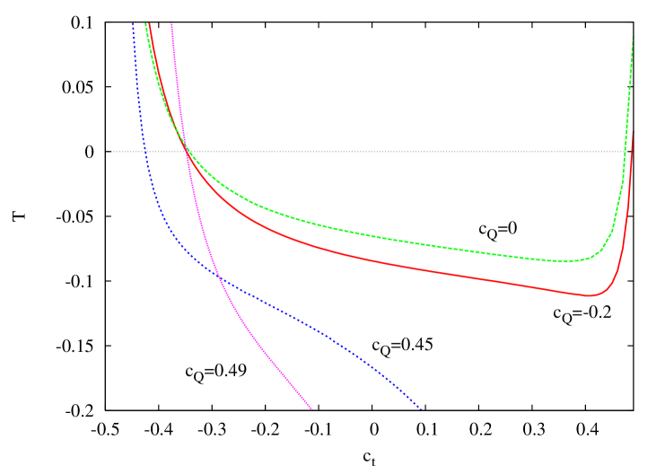
Figure 5: Contribution to the $T$ parameter involving the KK modes of the bidoublets and triplets which couple to the Higgs through the top Yukawa coupling, for the parity and quantum number assignments given in Eq. (33), We use $\tilde{k}=1.5~{}{\rm TeV}$ and $m_{\rm top}=167~{}{\rm GeV}$. It is assumed that the Higgs has the profile of gauge-Higgs unification models, Eq. (51).

For the cases that include triplets, as in Eq. (33), Eq. (3) has to be generalized to include the mixing within states of charge $5/3$, $2/3$ or $-1/3$. We show the $T$ parameter for this case in Fig. 5. The new ingredient is the presence of states, not part of a bidoublet, with parity assignments $(+,-)$ or $(-,+)$. This may lead to additional light states [18], and correspondingly important contributions to the $T$ parameter, depending on the value of $c_{t}$ (the discrete parity $P_{LR}$ implies that both triplets, $T_{1}$ and $T_{2}$, are controlled by the same localization parameter, which we call again $c_{t}$). For the parity assignments of the triplets in Eq. (33), that were motivated by the $SU(2)_{R}\times P_{LR}$ symmetry protecting $T$ and $\delta g_{b\,L}/g_{b\,L}$, the triplet states become light as $c_{t}\rightarrow 1/2$ (the RH zero mode is localized near the IR brane, and the first KK mode obeying $(-,+)$ boundary conditions for its RH components becomes light). These give a positive contribution to the $T$ parameter that explains the upward turn in the curves as $c_{t}\rightarrow 1/2$. In particular, the $T$ parameter can be positive in this region. Away from this region the triplet states are not particularly light and the behavior is similar to what was found for the assignments of Eq. (31): $T$ is dominated by a negative contribution due to the bidoublets, except near $c_{t}\sim-1/2$ (the conformal point for RH modes) where a large 5D Yukawa coupling enhances the mixing effects and the importance of various positive contributions (see the second term in Eq. (39), for example).

Thus, we see that the mechanism suggested in [8] to control the anomalous couplings of the bottom to the $Z$ implies a sizable negative contribution to the $T$ parameter in large regions of parameter space. There are, however, regions where $T$ can be positive. Given the positive $S$ parameter discussed in section 2.1, and that under these circumstances the EW data prefer positive values of the $T$ parameter, we conclude that the favored region has $c_{Q}$ not too close to $1/2$ and $c_{t}$ somewhere around $-0.4$ to $-0.5$ [or also around $0.5$ for models based on the assignment (33)].  We postpone a more detailed discussion of the EW constraints to the next section, where very similar bounds are found in the context of gauge-Higgs unification models. We will see that gauge bosons with KK masses around $3~{}{\rm TeV}$ are allowed. The most important lesson of this section is that the contribution to $T$ can be sufficiently important to select rather well-defined regions of parameter space, in this case the localization of the top quark multiplets in models based on $SU(2)_{L}\times SU(2)_{R}\times P_{LR}.$

Let us finish this section by mentioning that vector-like quarks as the ones present in these models also contribute to the $S$ parameter at one loop. Such a contribution is always positive and much less dependent on the parameters of the model. It is given by

$$S = \frac{N_{c}}{4\pi}\sum_{\alpha,\beta}\left[\left(U^{\dagger\alpha\beta}_{L}Y_{L}^{\beta\alpha}+U^{\dagger\alpha\beta}_{R}Y_{R}^{\beta\alpha}\right)\bar{\chi}_{+}(\mathcal{M}^{\mathrm{all}}_{\alpha\alpha},\mathcal{M}^{\mathrm{all}}_{\beta\beta})\right.$$ (47)

$$\hskip 105.2751pt\left.\mbox{}+\left(U^{\dagger\alpha\beta}_{L}Y_{R}^{\beta\alpha}+U^{\dagger\alpha\beta}_{R}Y_{L}^{\beta\alpha}\right)\bar{\chi}_{-}(\mathcal{M}^{\mathrm{all}}_{\alpha\alpha},\mathcal{M}^{\mathrm{all}}_{\beta\beta})\right]~{},$$

where

$$\bar{\chi}_{+}(y_{1},y_{2}) = \frac{5(y_{1}^{4}+y_{2}^{4})-22y_{1}^{2}y_{2}^{2}}{9(y_{1}^{2}-y_{2}^{2})^{2}}+\frac{3y_{1}^{2}y_{2}^{2}(y_{1}^{2}+y_{2}^{2})-(y_{1}^{6}+y_{2}^{6})}{3(y_{1}^{2}-y_{2}^{2})^{3}}\ln\left(\frac{y_{1}^{2}}{y_{2}^{2}}\right)-\frac{2}{3}\ln\left(\frac{y_{1}y_{2}}{\mu^{2}}\right)~{},$$

$$\bar{\chi}_{-}(y_{1},y_{2}) = \frac{y_{1}y_{2}}{(y_{1}^{2}-y_{2}^{2})^{3}}\left[y_{1}^{4}-y_{2}^{4}-2y_{1}^{2}y_{2}^{2}\ln\left(\frac{y_{1}^{2}}{y_{2}^{2}}\right)\right]~{}.$$ (48)

We assume that there are no exactly massless fermions in the theory. These would lead to IR divergences that need to be carefully subtracted. In the above, $\mu$ is an arbitrary scale that cancels out as a consequence of ${\rm Tr}[U^{\dagger}_{L}Y_{L}+U^{\dagger}_{R}Y_{R}]=0$, where $Y_{L,R}$ is the matrix of left- and right-handed hypercharge couplings in the mass eigenstate basis, while $U_{L,R}$ is the corresponding matrix of couplings to $W^{3}_{\mu}$. Note that in Eq. (47) we have put all fermion masses in a single (diagonal) matrix $\mathcal{M}^{\mathrm{all}}$. To obtain the contribution due to the new physics one needs to subtract the SM part. For example, the one due to the top-bottom system is

$$S_{\rm t,b}=-\frac{1}{6\pi}\left[\ln\left(\frac{m_{\rm top}^{2}}{m_{\rm bottom}^{2}}\right)-3\right]~{}.$$ (49)

We will include the phenomenological impact of this contribution to $S$ in the analysis of the next section.

4 Gauge-Higgs Unification

The models based on $SU(2)_{L}\times SU(2)_{R}\times U(1)_{X}$ discussed in the previous sections can be naturally embedded into $SO(5)\times U(1)_{X}$. The analysis of subsection 2.1 applies to this case by simply taking $g_{L}=g_{R}$. The additional gauge fields have the quantum numbers of the SM Higgs under $SU(2)_{L}\times SU(2)_{R}$ and offer the interesting possibility that the Higgs be part of a higher dimensional gauge field. This can help address the little hierarchy problem present in RS scenarios based on a fundamental scalar Higgs field. Imposing $(+,+)$ boundary conditions on the fifth component of the gauge fields in $SO(5)/SU(2)_{L}\times SU(2)_{R}$ allows one to identify the SM Higgs with their zero-mode components. One finds that these zero-modes have a nontrivial profile along the extra dimension

$$A^{\hat{a}}_{5}(x,y) = A^{\hat{a}(0)}_{5}(x)f_{H}(y)+\cdots$$ (50)

where $\hat{a}$ labels the generators of $SO(5)/SU(2)_{L}\times SU(2)_{R}$, and

$$f_{H}(y)=\left(\frac{2k}{e^{2kL}-1}\right)^{1/2}\,e^{2ky}~{}.$$ (51)

The Higgs field corresponds to the $SU(2)_{L}\times SU(2)_{R}$ bidoublet contained in the adjoint representation of $SO(5)$.

Regarding the fermion sector, the bidoublet plus singlet system of Eq. (31) fits into the fundamental representation of $SO(5)$,

$$5 \sim (2,2)\oplus 1~{},$$ (52)

while the system of a bidoublet and triplets of Eq. (33) fits into the 10-dimensional representation of $SO(5)$,

$$10 \sim (2,2)\oplus(3,1)\oplus(1,3)~{}.$$ (53)

Therefore, no fermions with quantum numbers different to those already encountered in the $SU(2)_{L}\times SU(2)_{R}$ theory studied in the previous sections are necessary. The results for the fermion loop contributions to the $T$ parameter can then be understood from the physics already discussed, with a couple of restrictions:

• A single bulk mass parameter controls simultaneously the localization of the bidoublet and singlet (or triplets) in a given $SO(5)$ multiplet.

• The Yukawa couplings are no longer free parameters, but are related to observed gauge couplings.

The SM fermions can be embedded in various ways into the above 5-dimensional $SO(5)$ structure. An economical way to do it is to let the SM singlet and doublet components of, say, the up-type sector arise from a single $SO(5)$ multiplet. That is, let the multiplets in Eqs. (31) or (33) come from the same $SO(5)$ multiplet:

$$\begin{array}[]{rclrclrcl}\xi^{5}&=&Q&\oplus&u\end{array}~{},$$ (55)

or

$$\begin{array}[]{rclrclrcl}\xi^{10}&=&Q&\oplus&T_{1}&\oplus&T_{2}\end{array}~{}.$$ (57)

In either case, the down-type sector must be assigned to a different $10$ of $SO(5)$. In these scenarios the up-type Yukawa couplings arise directly from the bulk gauge interactions, while the down-type Yukawa couplings can arise from mixing effects such as those discussed below.

It is instructive to consider the expression for the top Yukawa coupling in these cases. When both the LH and RH components of the top quark come from a $5$ of $SO(5)$, one finds

$$\lambda^{5}_{\rm top}=\frac{g_{4}}{\sqrt{2}}\left[\frac{(\frac{1}{4}-c^{2})2kLe^{2kL}}{(1-e^{(1-2c)kL})(1-e^{(1+2c)kL})}\right]^{1/2}~{},$$ (58)

where the factor of $1/\sqrt{2}$ arises from the normalization of the Higgs field. The factor in parenthesis arises from the integral over the extra dimension of the Higgs wavefunction, Eq. (51), times the fermion zero-mode wavefunctions ($c$ is the dimensionless mass parameter that controls the localization of the zero-modes). This factor reaches a maximum at $c=0$, and is exponentially suppressed for $|c|>1/2$. Taking $g_{4}\approx 0.65$, a running top quark mass of $167~{}{\rm GeV}$ is obtained for $|c|\approx 0.42$. For $c=0.42$, we can directly read the associated contribution to the $T$ parameter from Fig. 3 by setting $c_{1}=c_{2}=0.42$. For $\tilde{k}=1.5~{}{\rm TeV}$, which corresponds to gauge KK masses starting at $3.75~{}{\rm TeV}$, this gives $\Delta T\approx-0.08$. For $c=-0.42$ one finds $\Delta T\approx-0.25$.

If the top quark comes from a decouplet, one finds instead

$$\lambda^{10}_{\rm top}=\frac{1}{2\sqrt{2}}\lambda^{5}_{\rm top}~{}.$$ (59)

The factor of $1/2$ is an $SO(5)$ group theory factor, while the $1/\sqrt{2}$ comes from the normalization of the isospin-$0$ component of the $SU(2)_{R}$ triplet. For $c=0$, the maximum obtainable top mass is about $110~{}{\rm GeV}$, so that this scenario is ruled out.

A different possibility is to assign an independent $SO(5)$ multiplet for each SM model fermion. In this case, the gauge coupling, which is diagonal in flavor space, does not induce masses for the zero-modes. However, localized mass terms that mix different $SO(5)$ multiplets can generate the fermion masses and mixing angles, once the Higgs field gets a vev. Since the Higgs field is localized near the IR brane, see Eq. (51), only masses localized on the IR brane can be effective, and we may restrict ourselves to such cases. These masses preserve $SU(2)_{L}\times SU(2)_{R}$, so one may have localized masses that we call $\hat{M}_{Q}$ for the bidoublets, $\hat{M}_{u}$ for the singlets, and $\hat{M}_{T_{1}}$ and $\hat{M}_{T_{2}}$ for the triplets. Due to the localization, these “mass parameters” are dimensionless.

We are mainly interested in the fermion loop contributions to the $T$ parameter, thus we restrict ourselves again to the top quark sector (the contributions due to the other quark and lepton fields can be made negligibly small). A priori there are several ways of assigning the LH and RH top quark components to the $5$ and $10$ representations of $SO(5)$. However, due to the group theory factors associated with the 10-dimensional representation of $SO(5)$ it is impossible to accommodate the observed top mass unless the $SU(2)_{L}$ singlet top comes from a $5$. The $SU(2)_{L}$ doublet components can arise either from a $5$ or a $10$ of $SO(5)$. Therefore, in the top quark sector, only the bidoublet and singlet localized masses ($\hat{M}_{Q}$ and $\hat{M}_{u}$) are relevant.

The localized masses also affect the spectrum of KK modes and have the important consequence that they make the light states even lighter. Based on this observation we see that

• The bidoublet localized mass, $\hat{M}_{Q}$, by pushing the $\chi$ states to lower masses, has the effect of enhancing the negative contributions to the $T$ parameter discussed in section 3.

• The localized mass $\hat{M}_{u}$ can also generate light states in the singlet towers, which in general enhances their positive contributions to the $T$ parameter.

We find that whenever the bidoublet mass, $\hat{M}_{Q}$, is appreciable, the negative contributions to the $T$ parameter are very important. In fact, if the top mass is generated only from $\hat{M}_{Q}$, $T$ is negative for all $c_{1}$ and $c_{2}$, the localization parameters for the two $SO(5)$ multiplets that generate the top quark [12].

Given the restrictions imposed by the top quark mass, and in order to obtain positive values of $T$, we consider the case with only quintuplets of $SO(5)$, and choose the parities so that bidoublet mixing masses are forbidden:

$$\begin{array}[]{rcl}\xi_{1L}&\sim&\begin{array}[]{rclrcl}Q_{1L}&=&\begin{pmatrix}\chi^{u}_{1L}(-,+)&q^{u}_{L}(+,+)\\ \chi^{d}_{1L}(-,+)&q^{d}_{L}(+,+)\end{pmatrix}&\oplus&u^{\prime}_{L}(-,+)\end{array}~{},\\[15.00002pt] \xi_{2R}&\sim&\begin{array}[]{rclrcl}Q_{2R}&=&\begin{pmatrix}\chi^{u}_{2R}(+,-)&q^{\prime u}_{R}(+,-)\\ \chi^{d}_{2R}(+,-)&q^{\prime d}_{R}(+,-)\end{pmatrix}&\oplus&u_{R}(+,+)\end{array}~{},\end{array}$$ (64)

where, under $SU(2)_{L}\times SU(2)_{R}$, $Q_{i}\sim(2,2)$ for $i=1,2$, and $u$ and $u^{\prime}$ are singlets under this symmetry. All multiplets are taken to have charge $X=2/3$. The parities of $Q_{1}$ and $u$ are fixed by the unbroken $SU(2)_{R}$ symmetry on the IR brane, and by the low-energy content. The parities of $Q_{2}$ are chosen so the bidoublets cannot mix through IR brane localized masses, and the parity of $u^{\prime}$ is then fixed so a singlet mixing mass, that generates the top quark mass, can be written:

$$\delta(L-y)\left[\hat{M}_{u}\bar{u}^{\prime}_{L}u_{R}+{\rm h.c.}\right]~{}.$$ (65)

The parities of the remaining chiralities are opposite to the ones shown in Eq. (64).

This system is relatively simple to analyze. There are three fundamental parameters, $c_{1}$, $c_{2}$ and $\hat{M}_{u}$. Given $c_{1}$ and $c_{2}$, the top mass fixes $\hat{M}_{u}$. The top Yukawa coupling is given by

$$\lambda_{\rm top} \approx \frac{g_{4}}{\sqrt{2}}\hat{M}_{u}\left[\frac{(\frac{1}{2}-c_{1})(\frac{1}{2}+c_{2})2kLe^{2(1+c_{2}-c_{1})kL}}{(1-e^{(1-2c_{1})kL})(1-e^{(1+2c_{2})kL})}\right]^{1/2}$$ (66)

$$\quad\quad\quad\quad\mbox{}\times\left[1+\hat{M}_{u}^{2}\;e^{2(c_{2}-c_{1})kL}\;\frac{(\frac{1}{2}+c_{2})(1-e^{(1+2c_{1})kL})}{(\frac{1}{2}+c_{1})(1-e^{(1+2c_{2})kL})}\right]^{-1/2},$$

In the limit of small $\hat{M}_{u}$, the top Yukawa coupling is given by

$$\lambda_{\rm top}\approx\frac{g_{4}}{\sqrt{2}}\hat{M}_{u}\left[\frac{(\frac{1}{2}-c_{1})(\frac{1}{2}+c_{2})2kLe^{2(1+c_{2}-c_{1})kL}}{(1-e^{(1-2c_{1})kL})(1-e^{(1+2c_{2})kL})}\right]^{1/2}~{},$$ (67)

while for $\hat{M}_{u}\gg 1$ the singlet zero-mode lives in $\xi_{1}$, and the top Yukawa coupling reduces to Eq. (58) with $c=c_{1}$. In particular, it becomes independent of $c_{2}$. For given $c_{1,2}$, this last limit corresponds to the maximum achievable top Yukawa coupling. If $|c_{1}|$ is too large, it may be impossible to accommodate a large enough Yukawa coupling (for example, for $m_{\rm top}=167~{}{\rm GeV}$, one needs $|c_{1}|\begin{array}[]{c}\,\sim\vspace{-21pt}\\ <\end{array}0.42$, although mixing with light KK states can change this.) Therefore, the system contains two free parameters $c_{1}$ and $c_{2}$, where $|c_{1}|$ cannot be too close to $1/2$ in order to generate a sufficiently large top Yukawa coupling.

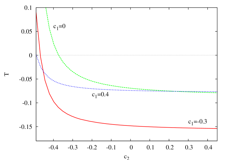
Figure 6: Contribution to the $T$ parameter involving the KK modes of Eq. (64), which couple to the Higgs through the top Yukawa coupling. We use $\tilde{k}=1.5~{}{\rm TeV}$ and $m_{\rm top}=167~{}{\rm GeV}$.

In Fig. 6 we plot the $T$ parameter as a function of $c_{2}$ for several values of $c_{1}$. We see that the situation is qualitatively similar to the case without gauge-Higgs unification presented in Fig 3, with $T$ negative for most values of $c_{2}$, and a rapid increase as $c_{2}$ approaches $-1/2$.

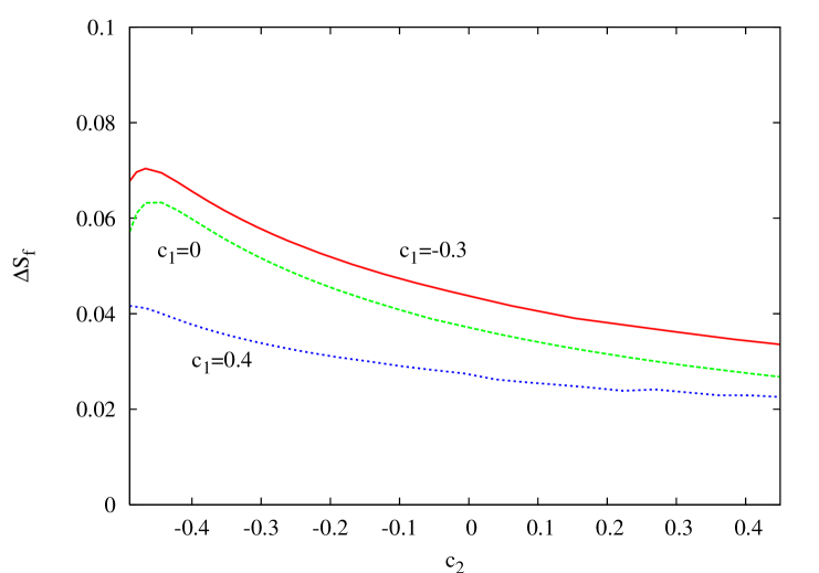
Figure 7: Contribution to the $S$ parameter involving the KK modes of Eq. (64), which couple to the Higgs through the top Yukawa coupling. We use $\tilde{k}=1.2~{}{\rm TeV}$ and $m_{\rm top}=167~{}{\rm GeV}$.

Given a positive $S$ parameter, and for small values of $U$, as is the case when the first two families are localized near the UV brane, the EW data prefer a positive value of $T$. We see in Fig. 6 that this restricts $c_{2}$ to be in the vicinity of $-0.4$ to $-0.5$, where $T$ crosses through zero. Thus, the most important constraints in the previous scenario come from the $T$ and $S$ parameters discussed in section 2.1, plus the extra contribution from the loops of fermion KK modes, Eq. (47). With the first two families near the UV brane (localization parameters for LH zero-modes, $c\begin{array}[]{c}\sim\vspace{-21pt}\\ >\end{array}0.55$ or so), the prediction for $S$ is

$$S\approx 9\,\frac{v^{2}}{\tilde{k}^{2}}+\Delta S_{f}~{},$$ (68)

where $\tilde{k}=ke^{-kL}$, and $\Delta S_{f}$ is the contribution from the fermion loops given in Eq. (47). In Fig. 7 we show $\Delta S_{f}$ as a function of $c_{2}$ for several values of $c_{1}$. We see that, as we said, it is positive and much less dependent on the parameters of the model.

For a light Higgs with $m_{H}\simeq 115~{}{\rm GeV}$ (recall that gauge-Higgs unification models typically predict a light Higgs), a $2\sigma$ bound on $S\begin{array}[]{c}\,\sim\vspace{-21pt}\\ <\end{array}0.3$ appears [20]. In order to be consistent with the $2\sigma$ $S$-$T$ bounds for the largest allowed values of $S$, a positive contribution of $T\approx 0.3$ is also required. The bound on $S$ leads to a lower bound $\tilde{k}\approx 1.2~{}{\rm TeV}$ (this includes a contribution $\Delta S_{f}\approx+0.06$), which corresponds to KK gauge boson masses of $M_{KK}\approx 2.5\,\tilde{k}\approx 3~{}{\rm TeV}$. In turn, the positive contribution to $T$ can arise from the 1-loop effects associated with the top sector discussed above, for specific values of the bulk mass parameters. For example, taking $c_{1}=0$, this can be obtained for $c_{2}=-0.468$. The top mass fixes $\hat{M}_{u}\approx 2.91$. The gauge contributions to the $T$ and $U$ parameters of Eq. (20) are negligible ($\Delta T_{\rm gauge}\approx-0.006$ and $\Delta U_{\rm gauge}\approx 0.005$).

For the above values of parameters, one also finds $\delta g_{b\,L}/g_{b\,L}\approx 0.8\times 10^{-3}$, arising from the gauge contribution in Eq. (25). There are also potentially important loop-level contributions to $\delta g_{b\,L}/g_{b\,L}$, involving the sector of fermion KK modes that mix with the top. In fact, in order to obtain a positive $T$ parameter this mixing needs to be relatively large. We have estimated this contribution using the results of [29], and obtained $\delta g^{\rm loop}_{b\,L}/g_{b\,L}\approx-5\times 10^{-3}$. The net value of $\delta g_{b\,L}/g_{b\,L}$ falls outside the range given in Eq. (22). A naive estimation, using only $R_{b}$, would seem to push the lower bound $\tilde{k}\approx 1.5$ TeV. A more careful analysis requires a global fit to all EW observables that is currently underway [12].

We conclude that there are rather well defined regions of parameter space that pass all current bounds from precision measurements with relatively light, and probably accessible at the LHC, gauge boson KK excitations. In fact, one typically finds fermion KK excitations, with masses below 1 TeV, that should give clear signals at the LHC, as we discuss next.

5 Phenomenology

We have seen in the previous sections how the $SU(2)$ custodial symmetry plus the $L\leftrightarrow R$ discrete symmetry allow for Randall-Sundrum models with KK excitations of the gauge bosons as low as $M_{KK}\sim 3$ TeV, mainly constrained by the $S$ parameter. In order to avoid large negative contributions to the $T$ parameter at the loop level, a very well defined pattern emerges, with the RH top quark not so strongly localized near the IR brane ($c_{2}\sim-0.4$ to $-0.5$, $-0.5$ being the conformal point for a RH fermion). We will focus on the gauge-Higgs unification model discussed in the previous section, with the quantum numbers and parities as in Eq. (64), and will outline the differences for other models at the end. The net positive contribution to the $T$ parameter in this case comes from a large positive contribution from a vector-like $SU(2)_{L}$ singlet that compensates a relatively large negative contribution from a light bidoublet ($c_{2}\sim-1/2$ localizes a LH zero mode near the IR brane, and the LH components of $Q_{2}$, that obey $(-,+)$ boundary conditions develop a light mode). Furthermore, the singlet is lighter than one would have expected from its localization parameter $c_{2}$ due to the effect of the localized mass $\hat{M}_{u}$. As an illustration, for the choice of parameters satisfying the EW constraints discussed above, one finds for the states with charges $5/3$ and $-1/3$, that do not mix through the Higgs vev:

$$M_{\chi^{u}_{2}}=M_{q^{\prime d}} \approx 470~{}{\rm GeV}~{}.$$ (69)

The lightest charge $2/3$ states, coming from $Q_{2}$, are split due to EW symmetry breaking effects. In fact, only one linear combination of $\chi^{d}_{2}$ and $q^{\prime u}$ mixes with the singlets. We call $q_{1}$ the linear combination that does not feel the Higgs vev. We call the two remaining states $q_{2}$ and $u_{2}$ (for a small Higgs vev, $q_{2}$ would be mostly an $SU(2)_{L}$ doublet while $u_{2}$ would be mostly an $SU(2)_{L}$ singlet). Their masses are

$$M_{q_{1}}\approx 470~{}{\rm GeV}~{},\hskip 28.45274ptM_{q_{2}}\approx 495~{}{\rm GeV}~{},\hskip 28.45274ptM_{u_{2}}\approx 742~{}{\rm GeV}~{}.$$ (70)

The mixing between the top quark and the latter mode is about $\sim 32\%$. There are additional fermion states starting at about $1.9~{}{\rm TeV}$.

Light vector-like quarks that mix strongly with the top have two main phenomenological effects. First, anomalous couplings of the SM quarks to the $Z$ and $W$ bosons [21] are induced due to mixing. For instance, in the numerical example we are considering the LH top coupling to the $Z$ and the $Wt_{L}b_{L}$ coupling are reduced by

$$\delta g_{Ztt}^{L}/g_{Ztt}^{L}\sim-0.2~{},\quad\delta g_{Wtb}^{L}/g_{Wtb}^{L}\sim-0.07~{},$$ (71)

The $Wt_{L}b_{L}$ coupling has not been directly measured yet. Early studies for single top production at the Tevatron [22] show that it may be measured with a precision of about 10 % for a total integrated luminosity of order 8 fb^-1. At the LHC, this coupling is expected to be measured to a $\sim 5$–$10\%$ precision [23]. Apart from the effect of the mixing with the fermion KK modes, there is an extra effect due to the mixing of the $Z$ with the gauge KK modes, similar to the one we discussed for the bottom couplings in section 2.1. Actually, the mechanism that protects the bottom quark coupling from corrections cannot simultaneously protect the top couplings [8]. Eq. (23) applies equally well to the top quark where we now have $T^{3}_{R}=-T^{3}_{L}=1(0)$ for the LH (RH) top quark chirality. This results in a very small modification of the RH coupling (recall that the one loop contribution to the $T$ parameter requires the RH top to leave not so close to the IR brane) whereas the LH coupling is modified by a factor

$$\delta g^{L(\mathrm{gauge})}_{Ztt}/g^{L}_{Ztt}\sim-0.04~{},$$ (72)

whereas the $Wt_{L}b_{L}$ coupling receives a correction

$$\delta g^{L(\mathrm{gauge})}_{Wtb}/g^{L}_{Wtb}\sim-0.015~{}.$$ (73)

As we see, this effect is smaller than the one coming from mixing with fermion KK modes. Apart from modifications of the diagonal top couplings, Flavor Changing Neutral Couplings (FCNC) are also generated both through mixing with vector-like quarks and due to the different top quark couplings in the gauge eigenstate basis that get mixed in the physical basis. These effects depend on the mixing with the first two families that we have not considered in detail here. The latter effect has been recently discussed in [24] with the result that FCNC possibly observable at the LHC can be generated. Recall, however, that due to the constraints associated with the $T$ parameter it is the LH top that is localized closer to the IR brane, and therefore it receives the largest modifications to its couplings. The authors of Ref. [24], instead, assumed that the largest effects appear in the RH sector.

Another phenomenological implication of light vector-like fermions is of course the possibility of direct production at colliders. The two relevant modes that are light and mix with the top are, in the gauge eigenstate basis, a bidoublet that is an equal admixture of a quark with isospin $+1/2$ and isospin $-1/2$ (and therefore its effects due to mixing are typically suppressed) and a singlet that mixes strongly with the top. Thus, as a first approximation we will consider the phenomenology of just the singlet. A more detailed analysis of the collider phenomenology of these and other fermion KK modes will be presented elsewhere [12].

Vector-like singlets of charge $2/3$ can be pair or singly produced at colliders. Pair production is quite independent of the heavy quark mixing with the top but the cross section dies off very quickly with the mass of the heavy quark. For instance, the production cross section of a 500 GeV quark at the Tevatron collider is about 1 fb [25], while it increases to values of a few pb at the LHC. Such small cross sections at the Tevatron imply that searches for these quarks, decaying mainly into third generation states, become quite challenging [25, 26]. Searches become much more promising at the LHC. A recent study [27] shows that a 500 GeV (1 TeV) vector-like quark singlet can be discovered at the LHC with an integrated luminosity of $\sim 1.2$ fb^-1 ($\sim 90$ fb^-1) thus rendering the signatures of our model easily observable.

Single production is not suppressed as much by the mass of the heavy quark but depends on the details of the mixing with the top-bottom sector. A comparison with the ATLAS study of little Higgs models [28] shows that a vector-like singlet with the parameters of our numerical example is well within LHC reach in single production. In particular the $T\to Wb$ channel looks particularly promising in the discovery of a quark with mass of order $750$ GeV and a $\sim 32\%$ mixing with the top. Furthermore, the mass of the singlet is typically light enough to make pair production competitive with single production.

We have thus seen that realistic models of gauge-Higgs unification with gauge KK excitations with masses as low as $3$ TeV can be constructed. Generic predictions of these models include deviations of the $Wtb$ coupling sufficiently large to be observed with the $\sim 5$–$10\%$ accuracy achievable at the LHC, as well as vector-like quarks light enough to be produced at the LHC, both in pairs and together with SM quarks. Alternative choices of quantum numbers and parities, but still compatible with EW precision observables, can have slightly different features regarding the spectrum of bidoublets, but light and strongly mixed vector-like singlets remain as a solid prediction of the models. If we relax the gauge-Higgs unification condition and allow for a fundamental Higgs as in sections 2 and 3, then vector-like singlets do not need to be that light. However, they still need to mix very strongly with the top to compensate for the negative contribution of bidoublets to the $T$ parameter. This typically results in a scenario with somewhat light vector-like bidoublets, with masses $M_{\chi}\sim 1$ TeV, and heavy vector-like singlets, with masses $M_{t}\sim 2.5$ TeV, which will be more challenging for the LHC. However, due to the strong mixing, large corrections to the top gauge couplings, in the $\sim 10-20\%$ range, and therefore observable at the LHC, are expected in these models.

6 Conclusions

The Randall-Sundrum scenario with gauge and fermion fields propagating in the bulk offers an attractive solution to the hierarchy problem, an understanding of the observed fermion hierarchies by extra-dimensional localization effects, and a natural suppression of dangerous flavor changing processes. A generic feature of these scenarios is that the third generation is quite different from the first two: by being closer to the IR brane the top quark avoids an exponential suppression in its mass, in contrast with the first two generation quarks and leptons, and can naturally be as heavy as the EW scale. One can then generically expect important deviations from the SM in this sector, most notably anomalous couplings to the $Z$ gauge boson, and contributions to the Peskin-Takeuchi $T$ parameter. The first two generations can also give important contributions to the $S$ parameter. These constraints tend to put the gauge boson KK excitations beyond the reach of the LHC, unless these states are lighter and more weakly coupled than expected, for example due to the presence of moderately large IR brane kinetic terms.

In the absence of brane localized terms, an $SU(2)_{L}\times SU(2)_{R}$ bulk gauge symmetry together with a discrete symmetry exchanging $L$ with $R$ [8] seem to be essential in bringing the contributions to the $T$ parameter, and the anomalous contributions to the $Z\bar{b}_{L}b_{L}$ vertex, under control. These symmetries, being broken non-locally by boundary conditions, imply that such effects are calculable. We have seen that they can still place important constraints on these models. A detailed calculation shows that the 1-loop contributions to the $T$ parameter are in general sizable. Furthermore, we have shown that the existence of $SU(2)_{L}\times SU(2)_{R}$ bidoublets, an essential ingredient in these scenarios, gives a negative contribution to the $T$ parameter. Contributions coming from singlets or triplets can compensate such effects, but the conspiracy occurs in rather well defined regions of parameter space. The $S$-$T$ constraints, in particular, very directly constrain the location of the third generation multiplets. In this regions, however, KK gauge excitations as light as $3~{}{\rm TeV}$ are allowed, thus providing the first example of RS scenarios with negligible brane localized terms, that are consistent with all EW precision data and with gauge boson KK states accessible at the LHC.

We also studied the EW constraints in models in which, in addition to the above structure, the Higgs arises from an extra-dimensional gauge field, thus alleviating the little hierarchy problem associated with a 5D scalar field. These scenarios contain further theoretical relations due to the embedding of the field content into larger gauge multiplets, as well as due to the fact that the Yukawa couplings are related to SM gauge couplings. In spite of these restrictions, we find that the EW measurements set bounds on the gauge boson KK masses of the order of 3 TeV, similar to those found in the absence of the gauge-Higgs unification assumption. An important difference, however, is that the required multiplet structure, together with the constraints on the location of the third family, typically lead to light vector-like fermionic excitations. Quite generically, a light $SU(2)_{L}$ singlet, that mixes with the top quark, is expected. Furthermore, it is likely that additional light $SU(2)_{L}$ doublet states, some of them with exotic charges, are present. All these states can easily have masses in the $500-800~{}{\rm GeV}$ range, and should be observable at the LHC, both by direct (single or pair) production and by their effect through mixing on the anomalous couplings of the top. Further fermionic excitations starting as low as $1-2~{}{\rm TeV}$ are also generically expected. All of these should provide interesting discovery signals and warrant a more detailed study of the associated phenomenology [12].

Acknowledgements
 
We would like to thank T. Tait for valuable conversations and collaboration at early stages of this work. We would also like to thank K. Agashe, J. Hubisz, B. Lillie and A. Pomarol for useful discussions and comments. Work at ANL is supported in part by the US DOE, Div. of HEP, Contract W-31-109-ENG-38. Fermilab is operated by Universities Research Association Inc. under contract no. DE-AC02-76CH03000 with the DOE. E.P. was supported by DOE under contract DE-FG02-92ER-40699.

References

- [1] L. Randall and R. Sundrum, Phys. Rev. Lett. 83, 3370 (1999) [arXiv:hep-ph/9905221].
- [2] M. E. Peskin and T. Takeuchi, Phys. Rev. D 46, 381 (1992).
- [3] S. J. Huber and Q. Shafi, Phys. Rev. D 63, 045010 (2001) [arXiv:hep-ph/0005286]; S. J. Huber, C. A. Lee and Q. Shafi, Phys. Lett. B 531, 112 (2002) [arXiv:hep-ph/0111465]; C. Csaki, J. Erlich and J. Terning, Phys. Rev. D 66, 064021 (2002) [arXiv:hep-ph/0203034]; J. L. Hewett, F. J. Petriello and T. G. Rizzo, JHEP 0209, 030 (2002) [arXiv:hep-ph/0203091].
- [4] M. Carena, E. Pontón, T. M. P. Tait and C. E. M. Wagner, Phys. Rev. D 67, 096006 (2003) [arXiv:hep-ph/0212307]; H. Davoudiasl, J. L. Hewett and T. G. Rizzo, Phys. Rev. D 68, 045002 (2003) [arXiv:hep-ph/0212279].
- [5] M. Carena, A. Delgado, E. Pontón, T. M. P. Tait and C. E. M. Wagner, Phys. Rev. D 68, 035010 (2003) [arXiv:hep-ph/0305188].
- [6] M. Carena, A. Delgado, E. Pontón, T. M. P. Tait and C. E. M. Wagner, Phys. Rev. D 71, 015010 (2005) [arXiv:hep-ph/0410344].
- [7] K. Agashe, A. Delgado, M. J. May and R. Sundrum, JHEP 0308, 050 (2003) [arXiv:hep-ph/0308036].
- [8] K. Agashe, R. Contino, L. Da Rold and A. Pomarol, arXiv:hep-ph/0605341.
- [9] N. S. Manton, Nucl. Phys. B 158, 141 (1979); Y. Hosotani, Phys. Lett. B 126, 309 (1983); H. Hatanaka, T. Inami and C. S. Lim, Mod. Phys. Lett. A 13, 2601 (1998) [arXiv:hep-th/9805067]; I. Antoniadis, K. Benakli and M. Quiros, New J. Phys. 3, 20 (2001) [arXiv:hep-th/0108005]; M. Kubo, C. S. Lim and H. Yamashita, Mod. Phys. Lett. A 17, 2249 (2002) [arXiv:hep-ph/0111327]; G. von Gersdorff, N. Irges and M. Quiros, Nucl. Phys. B 635, 127 (2002) [arXiv:hep-th/0204223]; C. Csaki, C. Grojean and H. Murayama, Phys. Rev. D 67, 085012 (2003) [arXiv:hep-ph/0210133]; N. Haba, M. Harada, Y. Hosotani and Y. Kawamura, Nucl. Phys. B 657, 169 (2003) [Erratum-ibid. B 669, 381 (2003)] [arXiv:hep-ph/0212035]; C. A. Scrucca, M. Serone and L. Silvestrini, Nucl. Phys. B 669, 128 (2003) [arXiv:hep-ph/0304220]; C. A. Scrucca, M. Serone, L. Silvestrini and A. Wulzer, JHEP 0402, 049 (2004) [arXiv:hep-th/0312267]; N. Haba, Y. Hosotani, Y. Kawamura and T. Yamashita, Phys. Rev. D 70, 015010 (2004) [arXiv:hep-ph/0401183]; C. Biggio and M. Quiros, Nucl. Phys. B 703, 199 (2004) [arXiv:hep-ph/0407348]; Y. Hosotani, S. Noda and K. Takenaga, Phys. Lett. B 607, 276 (2005) [arXiv:hep-ph/0410193]; G. Cacciapaglia, C. Csaki and S. C. Park, JHEP 0603, 099 (2006) [arXiv:hep-ph/0510366]; G. Panico, M. Serone and A. Wulzer, Nucl. Phys. B 739, 186 (2006) [arXiv:hep-ph/0510373]; G. Panico, M. Serone and A. Wulzer, arXiv:hep-ph/0605292.
- [10] K. Agashe, R. Contino and A. Pomarol, Nucl. Phys. B 719, 165 (2005) [arXiv:hep-ph/0412089];
- [11] S. J. Huber, arXiv:hep-ph/0211056; S. J. Huber, Nucl. Phys. B 666 (2003) 269 [arXiv:hep-ph/0303183]. K. Agashe, G. Perez and A. Soni, arXiv:hep-ph/0406101; arXiv:hep-ph/0408134.
- [12] M. Carena, E. Pontón, J. Santiago and C. E. M. Wagner, in preparation
- [13] H. E. Haber and H. E. Logan, Phys. Rev. D 62, 015011 (2000) [arXiv:hep-ph/9909335].
- [14] D. Choudhury, T. M. P. Tait and C. E. M. Wagner, Phys. Rev. D 65, 053002 (2002) [arXiv:hep-ph/0109097].
- [15] K. Agashe and R. Contino, Nucl. Phys. B 742, 59 (2006) [arXiv:hep-ph/0510164].
- [16] L. Lavoura and J. P. Silva, Phys. Rev. D 47, 2046 (1993).
- [17] H. Davoudiasl, B. Lillie and T. G. Rizzo, arXiv:hep-ph/0508279.
- [18] K. Agashe and G. Servant, “Baryon number in warped GUTs: Model building and (dark matter related) JCAP 0502, 002 (2005) [arXiv:hep-ph/0411254].
- [19] J. Hirn and V. Sanz, arXiv:hep-ph/0606086.
- [20] [ALEPH Collaboration], Phys. Rept. 427, 257 (2006) [arXiv:hep-ex/0509008].
- [21] F. del Aguila, M. Perez-Victoria and J. Santiago, JHEP 0009, 011 (2000) [arXiv:hep-ph/0007316]; F. del Aguila and J. Santiago, JHEP 0203, 010 (2002) [arXiv:hep-ph/0111047]; J. A. Aguilar-Saavedra, Phys. Rev. D 67, 035003 (2003) [Erratum-ibid. D 69, 099901 (2004)] [arXiv:hep-ph/0210112].
- [22] D. Amidei et al. [TeV-2000 Study Group], SLAC-REPRINT-1996-085
- [23] G. Altarelli and M. L. Mangano, CERN-2000-004
- [24] K. Agashe, G. Perez and A. Soni, arXiv:hep-ph/0606293.
- [25] T. C. Andre and J. L. Rosner, Phys. Rev. D 69, 035009 (2004) [arXiv:hep-ph/0309254].
- [26] D. E. Morrissey and C. E. M. Wagner, Phys. Rev. D 69, 053001 (2004) [arXiv:hep-ph/0308001].
- [27] J. A. Aguilar-Saavedra, Phys. Lett. B 625, 234 (2005) [Erratum-ibid. B 633, 792 (2006)] [arXiv:hep-ph/0506187]; J. A. Aguilar-Saavedra, PoS TOP2006, 003 (2006) [arXiv:hep-ph/0603199].
- [28] D. Costanzo, ATL-PHYS-2004-004; G. Azuelos et al., Eur. Phys. J. C 39S2, 13 (2005) [arXiv:hep-ph/0402037].
- [29] P. Bamert, C. P. Burgess, J. M. Cline, D. London and E. Nardi, Phys. Rev. D 54, 4275 (1996) [arXiv:hep-ph/9602438].