Mass Uncertainties of $f_{0}(600)$ and $f_{0}(1370)$ and their Effects on Determination of the Quark and Glueball Admixtures of the $I=0$ Scalar Mesons

Abstract

Within a nonlinear chiral Lagrangian framework the correlations between the quark and glueball admixtures of the isosinglet scalar mesons below 2 GeV and the current large uncertainties on the mass of the $f_{0}(600)$ and the $f_{0}(1370)$ are studied. The framework is formulated in terms of two scalar meson nonets (a two-quark nonet and a four-quark nonet) together with a scalar glueball. It is shown that while some properties of these states are sensitive to the mass of $f_{0}(600)$ and $f_{0}(1370)$, several relatively robust conclusions can be made: The $f_{0}(600)$, the $f_{0}(980)$, and the $f_{0}(1370)$ are admixtures of two and four quark components, with $f_{0}(600)$ being dominantly a non-strange four-quark state, and $f_{0}(980)$ and $f_{0}(1370)$ having a dominant two-quark component. Similarly, the $f_{0}(1500)$ and the $f_{0}(1710)$ have considerable two and four quark admixtures, but in addition have a large glueball component. For each state, a detailed analysis providing the numerical estimates of all components is given. It is also shown that this framework clearly favors the experimental values: $m^{\rm exp.}[f_{0}(600)]<700$ MeV and $m^{\rm exp.}[f_{0}(1370)]$ = 1300$-$1450 MeV. Moreover, an overall fit to the available data shows a reciprocal substructure for the $f_{0}(600)$ and the $f_{0}(1370)$, and a linear correlation between their masses of the form $m[f_{0}(1370)]=0.29\,m[f_{0}(600)]+1.22$ GeV. The scalar glueball mass of 1.5$-$1.7 GeV is found in this analysis.

I Introduction

Exploring the properties of the scalar mesons is known to be a non trivial task in low energy QCD. This is due to issues such as their large decay widths and overlap with the background, as well as having several decay channels over a tight energy range PDG . Particularly, the case of $I=0$ states is even more complex due to their various mixings, for example, among two and four quark states and scalar glueballs. Below 1 GeV, the well-established experimental states are PDG : the $f_{0}(980)$ [$I=0$] and the $a_{0}(980)$ [$I=1$], together with states that have uncertain properties: the $f_{0}(600)$ or $\sigma$ [$I=0$] with a mass of 400$-$1200 MeV, and a decay width of 600$-$1000 MeV, and the $K_{0}^{*}(800)$ or $\kappa$ [$I=1/2$] which is not yet listed but cautiously discussed in PDG. The existence of the $K_{0}^{*}(800)$ has been confirmed in some theoretical models, while has been disputed in some other approaches. In the range of 1$-$2 GeV, the listed scalar states are PDG : $K_{0}^{*}(1430)$ [$I=1/2$]; $a_{0}(1450)$ [$I=1$]; and $f_{0}(1370)$, $f_{0}(1500)$, $f_{0}(1710)$ [$I=0$]. The isodoublet and isotriplet states, are generally believed to be closer to $q{\bar{q}}$ objects, even though some of their properties significantly deviate from such a description. Among the heavier isosinglet states, the $f_{0}(1370)$ has the largest experimental uncertainty PDG on its mass (1200$-$1500 MeV) and decay width (200$-$500 MeV), and other states in the energy range of around 1.5 GeV (or above) seem to contain a large glue component and maybe good candidates for the lowest scalar glueball state.

A simple quark-antiquark description is known to fail for the lowest-lying scalar states, and that has made them the focus of intense investigation for a long time. Several foundational scenarios for their substructures have been considered, including MIT bag model Jaf , $K{\bar{K}}$ molecule Isg and unitarized quark model Tor , and many theoretical frameworks for the properties of the scalars have been developed, including, among others, chiral Lagrangian of refs. San ; BFSS1 ; BFSS2 ; Far ; pieta ; Mec ; LsM ; 02_BHS ; Higgs ; e3p ; 04_F1 ; 04_F2 ; 05_FJS , upon which the present investigation is based. Many recent works Eli ; 00_CK ; 02_CT ; 02_TKM ; 04_TKM ; 04_NR ; 05_GGF ; 05_GGLF ; 05_VVFS ; 05_BNNB ; 05_N ; 06_MPPR have investigated different aspects of the scalar mesons, particularly, their family connections and possible description in terms of meson nonet(s), which proved a comparison with this work.

Various ways of grouping the scalars together have been considered in the literature. For example, in some approaches, the properties of the scalars above 1 GeV (independent of the states below 1 GeV) are investigated, whereas other works have only focused on the states below 1 GeV. There are also works that have investigated several possibilities for grouping together some of the states above 1 GeV with those below 1 GeV.

In addition to various ways that the physical states may be grouped together, different bases out of quark-antiquark, four quark, and glueball have been considered for their internal structure. For example, in a number of investigations the $I=0$ states above 1 GeV are studied within a framework which incorporates quark-antiquark and glueball components. However, in lack of a complete framework for understanding the properties of the scalar mesons it seems more objective to develop general frameworks in which, a priori, no specific substructure for the scalars is assumed, and instead, all possible components (quark-antiquark, four-quark, and glueball) are considered. The framework of the present work considers all such components for the $I=0$ states, and studies the five listed $I=0$ states below 2 GeV PDG .

Besides the generality of the framework, there are supportive indications that the lowest and the next-to-lowest lying scalar states have admixtures of quark-antiquark and four-quark components. For example, it is shown in Mec that the $a_{0}(1450)$ and the $K_{0}^{*}(1430)$ have a considerable two and four quark admixtures, which provides a basis for explaining the mass spectrum and the partial decay widths of the $I=1/2$ and $I=1$ scalars [$K_{0}^{*}(800),a_{0}(980),K_{0}^{*}(1430)$ and $a_{0}(1450)$]. It then raises the question that if the $I=1/2$ and $I=1$ scalars below 2 GeV are admixtures of two and four quark components, why should not the $I=0$ states be blurred with such a mixing complexity? Answering this question is the main motivation of this paper, and we will see that this framework shows that there is a substantial admixture of the two and the four quark components for the $I=0$ scalars below 2 GeV.

Motivated by the importance of the mixing for the $I=1/2$ and $I=1$ in this framework, the case of the $I=0$ states was initially studied in 04_F1 ; 04_F2 in which mixing with a scalar glueball is also included. In 04_F1 the parameter space of the $I=0$ Lagrangian, which is already constrained by the properties of the $I=1/2$ and $I=1$ states in ref. Mec , is studied using the mass spectrum and several two-pseudoscalar decay widths and decay ratios of the $I=0$ states. The present work extends the work of 04_F1 by investigating in detail the effect of the mass uncertainties of the $f_{0}(600)$ and $f_{0}(1370)$ on the components of the $I=0$ states below 2 GeV. It also provides an insight into the likelihood of the mass of $f_{0}(600)$ and $f_{0}(1370)$ within their experimental values PDG in ranges 400-1200 MeV and 1200-1500 MeV, respectively. In addition a linear correlation between these two masses is predicted by the model.

Specifically, we will numerically analyze the mass spectrum and perform an inverse problem: knowing the mass of the physical states (or in the case of the $f_{0}(600)$ and the $f_{0}(1370)$ a wide experimental range for their masses) we search for the parameter space of the Lagrangian (which is formulated in terms of a two quark nonet and a four quark nonet) and find solutions that can reproduce these masses. Once the parameter space is determined it provides information about the properties of the two nonets. The results are summarized in Fig.1. We will show how the present model describes the $I=0$ scalar states in terms of a four-quark nonet $N$ which lies in the range of 0.83-1.24 GeV, together with a two-quark nonet $N^{\prime}$ in the 1.24-1.38 GeV range, and a scalar glueball that this model predicts in the range of 1.5-1.7 GeV (figure 1). The mass range of the two quark scalar nonet $N^{\prime}$ is qualitatively consistent with the expected range of 1.2 GeV from spectroscopy of $p$-wave mesons. We will see that this analysis shows that, similar to the case of $I=1/2$ and $I=1$ scalar mesons, the $I=0$ scalars have a significant admixtures of two and four quark components, and in addition the $f_{0}(1500)$ and the $f_{0}(1710)$ have a dominant glueball content. The dominant component(s) of each state is summarized in Fig. 1.

The underlying framework of the present work has been previously applied in analyzing numerous low-energy processes that involve scalar mesons, and consistent pictures have emerged. The existence of the $f_{0}(600)$ (or $\sigma$) and the $K_{0}^{*}(800)$ (or $\kappa$) and their properties have been investigated in refs. San ; BFSS1 . The lowest-lying nonet of scalars and a four-quark interpretation of these states is studied in BFSS2 and applied to $\pi\eta$ scattering in pieta and several decays such as $\eta^{\prime}\rightarrow\eta\pi\pi$ Far and $\eta\rightarrow 3\pi$ e3p and radiative $\phi$ decays 02_BHS . In addition to ref. Mec , the mixing between a two quark and a four quark nonets is also investigated in LsM and 05_FJS .

We describe the theoretical framework in Sec. 1, followed by the numerical results in Sec.2, and a short summary in Sec. 3.

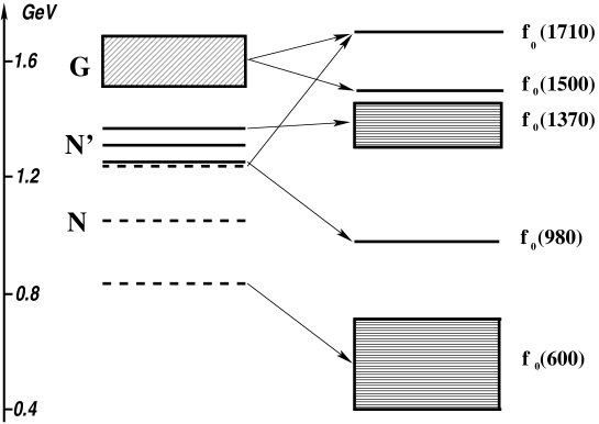
Figure 1: Prediction of the present model for the formation of the $I=0$ scalar states below 2 GeV. On the right, the physical states are shown, with the solid lines representing the experimentally well established masses, and the height of the two boxes representing the prediction of the present model for the uncertainties of the mass of $f_{0}(600)$ and $f_{0}(1370)$, which are approximately in ranges 0.4 - 0.7 GeV and 1.3 - 1.45 GeV, respectively. On the left, the “bare” states are shown, with the dashed lines representing the four-quark nonet $N$, the solid lines representing the two-quark nonet $N^{\prime}$ and the box representing the scalar glueball. The mass of the bare states in the two nonets (from bottom to top) are: $m({\bar{u}}{\bar{d}}ud)$ = 0.83 GeV, $m({\bar{d}}{\bar{s}}ud)$ = 1.06 GeV, $m({\bar{s}}{\bar{d}}ds+{\bar{s}}{\bar{u}}us)/\sqrt{2})=m({\bar{u}}u+{\bar{d}}d)/\sqrt{2})$ = 1.24 GeV, $m({\bar{u}}s)$ = 1.31 GeV and $m({\bar{s}}s)$ = 1.38 GeV. The uncertainty of the glueball mass (shown by the height of the box, approximately between 1.5 GeV to 1.7 GeV) is due to the uncertainty of the mass of $f_{0}(600)$ and $f_{0}(1370)$. The arrows show the dominant component(s) of each physical state. More details are given in Figs. 7 and 8.

II Theoretical Framework

II.1 Mixing Mechanism for I=1/2 and I=1 Scalar States

In ref. Mec the properties of the $I=1/2$ and $I=1$ scalar mesons, $\kappa(900)$, $K_{0}^{*}(1430)$, $a_{0}(980)$ and $a_{0}(1450)$, in a nonlinear chiral Lagrangian framework is studied in detail. In this approach, a ${\bar{q}}{\bar{q}}qq$ nonet $N$ mixes with a ${\bar{q}}q$ nonet $N^{\prime}$ and provides a description of the mass spectrum and decay widths of these scalars. The $K_{0}^{*}(1430)$ and the $a_{0}(1450)$, are generally believed to be good candidates for a ${\bar{q}}q$ nonet PDG , but some of their properties do not quite follow this scenario. For example, in a $q{\bar{q}}$ nonet, isotriplet is expected to be lighter than the isodoublet, but for these two states PDG :

$$m\left[a_{0}(1450)\right]=1474\pm 19\hskip 5.69046pt{\rm MeV}>m\left[K_{0}^{*}(1430)\right]=1412\pm 6\hskip 5.69046pt{\rm MeV}$$ (1)

Also their decay ratios given in PDG PDG do not follow a pattern expected from an SU(3) symmetry (given in parenthesis):

$${{\Gamma\left[a_{0}^{total}\right]}\over{\Gamma\left[K_{0}^{*}\rightarrow\pi K\right]}} = 0.92\pm 0.12\hskip 5.69046pt(1.51)$$

$$\hskip 5.69046pt{{\Gamma\left[a_{0}\rightarrow K{\bar{K}}\right]}\over{\Gamma\left[a_{0}\rightarrow\pi\eta\right]}} = 0.88\pm 0.23\hskip 5.69046pt(0.55)$$

$$\hskip 5.69046pt{{\Gamma\left[a_{0}\rightarrow\pi\eta^{\prime}\right]}\over{\Gamma\left[a_{0}\rightarrow\pi\eta\right]}} = 0.35\pm 0.16\hskip 5.69046pt(0.16)$$ (2)

These properties of the $K_{0}^{*}(1430)$ and the $a_{0}(1450)$ are naturally explained by the mixing mechanism of ref. Mec . The general mass terms for the $I=1/2$ and the $I=1$ states can be written as

$${\cal L}_{mass}^{I=1/2,1}=-a{\rm Tr}(NN)-b{\rm Tr}(NN{\cal M})-a^{\prime}{\rm Tr}(N^{\prime}N^{\prime})-b^{\prime}{\rm Tr}(N^{\prime}N^{\prime}{\cal M})$$ (3)

where ${\cal M}={\rm diag}(1,1,x)$ with $x$ being the ratio of the strange to non-strange quark masses, and $a,b,a^{\prime}$ and $b^{\prime}$ are unknown parameters fixed by the unmixed or “bare” masses (denoted below by subscript “0”):

$$\begin{array}[]{cclcccl}m^{2}[a_{0}]&=&2(a+b)&&m^{2}[a^{\prime}_{0}]&=&2(a^{\prime}+b^{\prime})\\ m^{2}[K_{0}]&=&2a+(1+x)b&&m^{2}[K^{\prime}_{0}]&=&2a^{\prime}+(1+x)b^{\prime}\end{array}$$ (4)

As $N$ is a four-quark nonet and $N^{\prime}$ a two-quark nonet, we expect:

$$m^{2}[K_{0}]<m^{2}[a_{0}]\leq m^{2}[a^{\prime}_{0}]<m^{2}[K^{\prime}_{0}]$$ (5)

In fact, this is how we tag $N$ and $N^{\prime}$ to a four-quark and a two-quark nonet, respectively. Introducing a general mixing

$${\cal L}_{mix}^{I=1/2,1}=-\gamma{\rm Tr}\left(NN^{\prime}\right)$$ (6)

it is shown in Mec that for $0.51<\gamma<0.62\hskip 5.69046pt{\rm GeV^{2}}$, it is possible to recover the physical masses such that the “bare” masses have the expected ordering of (5). In this mechanism, the “bare” isotriplet states split more than the isodoublets, and consequently, the physical isovector state $a_{0}(1450)$ becomes heavier than the isodoublet state $K_{0}^{*}(1430)$ in agreement with the observed experimental values in (1). The light isovector and isodoublet states are the $a_{0}(980)$ and the $K_{0}^{*}(800)$. With the physical masses $m[a_{0}(980)]=0.9835$ GeV, $m[K_{0}^{*}(800)]=0.875$ GeV, $m[a_{0}(1450)]=1.455$ GeV and $m[K_{0}(1430)]=1.435$ GeV, the best values of mixing parameter $\gamma$ and the “bare” masses are found in Mec

$$m_{a_{0}}=m_{a^{\prime}_{0}}=1.24\hskip 2.84544pt{\rm GeV},\hskip 5.69046ptm_{K_{0}}=1.06\hskip 2.84544pt{\rm GeV},\hskip 5.69046ptm_{K^{\prime}_{0}}=1.31\hskip 2.84544pt{\rm GeV},\hskip 5.69046pt\gamma=0.58\hskip 2.84544pt{\rm GeV^{2}}$$ (7)

These parameters are then used to study the decay widths of the $I=1/2$ and $I=1$ states Mec . A general Lagrangian describing the coupling of the two nonets $N$ and $N^{\prime}$ to two-pseudoscalar particles are introduced and the unknown Lagrangian parameters are found by fits to various decay widths.

In summary, the work of ref. Mec clearly shows that properties of the lowest and the next-to-lowest $I=1/2$ and $I=1$ scalar states can be described by a mixing between a quark-antiquark nonet and a four quark nonet. It is concluded that the $I=1$ states are close to maximal mixing (i.e. $a_{0}(980)$ and $a_{0}(1450)$ are approximately made of 50% quark-antiquark and 50% four-quark components), and the $I=1/2$ states have a similar structure with $K_{0}^{*}(800)$ made of approximately 74% of four-quark and 26% quark-antiquark, and the reverse structure for the $K_{0}^{*}(1430)$. Now if the lowest and the next-to-lowest $I=1/2$ and $I=1$ states have a substantial mixing of quark-antiquark and four-quark components, then it seems necessary to investigate a similar scenario for the $I=0$ scalars, which, in addition, can have a glueball component as well. In other words, if the lowest and the next-to-lowest scalars are going to be grouped together, then all components of quark-antiquark, four-quark and glueball for the $I=0$ states should be taken into account. The case of $I=0$ states will be discussed in next section.

II.2 Isosinglet States

The $I=0$ scalars have been investigated in many recent works, including the general approach with two and four quark components as well as a glueball component of refs. 04_F1 ; 04_F2 . Within the framework of ref. Mec , an initial analysis is given in 04_F1 in which the mass and the decay Lagrangian for the $I=0$ scalar mesons are studied in some details. The general mass terms for nonets $N$ and $N^{\prime}$, and a scalar glueball $G$ can be written as:

$${\cal L}_{mass}^{I=0} = {\cal L}_{mass}^{I=1/2,1}-c{\rm Tr}(N){\rm Tr}(N)-d{\rm Tr}(N){\rm Tr}(N{\cal M})$$ (8)

$$-c^{\prime}{\rm Tr}(N^{\prime}){\rm Tr}(N^{\prime})-d^{\prime}{\rm Tr}(N^{\prime}){\rm Tr}(N^{\prime}{\cal M})-gG^{2}$$

The unknown parameters $c$ and $d$ induce “internal” mixing between the two $I=0$ flavor combinations [$(N_{1}^{1}+N_{2}^{2})/\sqrt{2}$ and $N_{3}^{3}$] of nonet $N$. Similarly, $c^{\prime}$ and $d^{\prime}$ play the same role in nonet $N^{\prime}$. Parameters $c,d,c^{\prime}$ and $d^{\prime}$ do not contribute to the mass spectrum of the $I=1/2$ and $I=1$ states. The last term represents the glueball mass term. The term ${\cal L}_{mass}^{I=1/2,1}$ is imported from Eq. (3) together with its parameters from Eq. (7).

The mixing between $N$ and $N^{\prime}$, and the mixing of these two nonets with the scalar glueball $G$ can be written as

$${\cal L}_{mix}^{I=0}={\cal L}_{mix}^{I=1/2,1}-\rho{\rm Tr}(N){\rm Tr}(N^{\prime})-eG{\rm Tr}\left(N\right)-fG{\rm Tr}\left(N^{\prime}\right)$$ (9)

where the first term is given in (6) with $\gamma$ from (7). The second term does not contribute to the $I=1/2,1$ mixing, and in special limit of $\rho\to-\gamma$:

$$-\gamma{\rm Tr}(NN^{\prime})-\rho{\rm Tr}(N){\rm Tr}(N^{\prime})=\gamma\epsilon^{abc}\epsilon_{ade}N^{d}_{b}{N^{\prime}}^{e}_{c}$$ (10)

which is more consistent with the OZI rule than the individual $\gamma$ and $\rho$ terms and is studied in 02_TKM . Here we do not restrict the mixing to this particular combination, and instead, take $\rho$ as a a priori unknown free parameter. Terms with unknown couplings $e$ and $f$ describe mixing with the scalar glueball $G$. As a result, the five isosinglets below 2 GeV, become a mixture of five different flavor combinations, and their masses can be organized as

$${\cal L}_{mass}^{I=0}+{\cal L}_{mix}^{I=0}=-{1\over 2}{\tilde{\bf F}}_{0}{\bf M}^{2}{\bf F}_{0}=-{1\over 2}{\tilde{\bf F}}{\bf M}_{diag.}^{2}{\bf F}$$ (11)

with

$${\bf F}_{0}=\begin{array}[]{l}\left(\begin{array}[]{c}N_{3}^{3}\\ (N_{1}^{1}+N_{2}^{2})/\sqrt{2}\\ {N^{\prime}}_{3}^{3}\\ ({N^{\prime}}_{1}^{1}+{N^{\prime}}_{2}^{2})/\sqrt{2}\\ G\end{array}\right)\par\end{array}=\begin{array}[]{l}\left(\begin{array}[]{c}{\bar{u}}{\bar{d}}ud\\ ({\bar{s}}{\bar{d}}ds+{\bar{s}}{\bar{u}}us)/\sqrt{2}\\ {\bar{s}}s\\ ({\bar{u}}u+{\bar{d}}d)/\sqrt{2}\\ G\end{array}\right)\par\end{array}=\begin{array}[]{l}\left(\begin{array}[]{l}f_{0}^{NS}\\ f_{0}^{S}\\ {f^{\prime}}_{0}^{S}\\ {f^{\prime}}_{0}^{NS}\\ G\end{array}\right)\end{array}$$ (12)

where the superscript $NS$ and $S$ respectively represent the non-strange and strange combinations. ${\bf F}$ contains the physical fields

$${\bf F}=\begin{array}[]{c}\left(\begin{array}[]{c}\sigma(550)\\ f_{0}(980)\\ f_{0}(1370)\\ f_{0}(1500)\\ f_{0}(1710)\end{array}\right)=K^{-1}{\bf F}_{0}\end{array}$$ (13)

where $K^{-1}$ is the transformation matrix. The mass squared matrix is

$${\bf M}^{2}=\left[\begin{array}[]{ccccc}2m_{K_{0}}^{2}-m_{a_{0}}^{2}+2(c+dx)&\sqrt{2}[2c+(1+x)d]&\gamma+\rho&\sqrt{2}\rho&e\\ \sqrt{2}[2c+(1+x)d]&m_{a_{0}}^{2}+4(c+d)&\sqrt{2}\rho&\gamma+2\rho&\sqrt{2}e\\ \gamma+\rho&\sqrt{2}\rho&2m_{K^{\prime}_{0}}^{2}-m_{a^{\prime}_{0}}^{2}+2(c^{\prime}+d^{\prime}x)&\sqrt{2}[2c^{\prime}+(1+x)d^{\prime}]&f\\ \sqrt{2}\rho&\gamma+2\rho&\sqrt{2}[2c^{\prime}+(1+x)d^{\prime}]&m_{a^{\prime}_{0}}^{2}+4(c^{\prime}+d^{\prime})&\sqrt{2}f\\ e&\sqrt{2}e&f&\sqrt{2}f&2g\end{array}\right]$$ (14)

in which the value of the unmixed $I=1/2,1$ masses, and the mixing parameter $\gamma$ are substituted in from (7). We see that there are eight unknown parameters in (14) which are $c$, $d$, $c^{\prime}$, $d^{\prime}$, $g$, $\rho$, $e$ and $f$. We will use numerical analysis to search this eight dimensional parameter space for the best values that give closest agreement with experimentally known masses. Particularly, we will study in detail the effect of the large uncertainties on the mass of the $f_{0}(600)$ and $f_{0}(1370)$ on the resulting parameters.

III Matching the Theoretical Prediction to Experimental Data

To determine the eight unknown Lagrangian parameters ($c,c^{\prime},d,d^{\prime},e,f,g$ and $\rho$), we input the experimental masses of the scalar states. Out of the five isosignlet states, three have a well established experimental mass PDG :

$$\begin{array}[]{r c l}m^{\rm exp.}[f_{0}(980)]&=&980\pm 10\,{\rm MeV}\\ m^{\rm exp.}[f_{0}(1500)]&=&1507\pm 5\,{\rm MeV}\\ m^{\rm exp.}[f_{0}(1710)]&=&1713\pm 6\,{\rm MeV}\end{array}$$ (15)

However, the experimental mass of the $f_{0}(600)$ and the $f_{0}(1370)$ have very large uncertainties PDG :

$$m^{\rm exp.}[f_{0}(600)] = 400\rightarrow 1200\,\,{\rm MeV}$$

$$m^{\rm exp.}[f_{0}(1370)] = 1200\rightarrow 1500\,\,{\rm MeV}$$ (16)

We search for the eight Lagrangian parameters (which in turn determine the mass matrix (14)) such that three of the resulting eigenvalues match their central experimental values in (15), and the other two masses fall somewhere in the experimental ranges in (16). This means that out of the five eigenvalues of (14), three (eigenvalues 2, 4 and 5) should match the fixed target values in (15), but two (eigenvalues 1 and 3) have no fixed target values and instead can be match to any values in (16). Therefore, to include all possibilities for the experimental ranges in (16), we numerically scan the $m^{\rm exp.}[f_{0}(600)]$$-$$m^{\rm exp.}[f_{0}(1370)]$ plane over the allowed ranges, and at each point we fit for the eight Lagrangian parameters such that the three theoretically calculated eigenvalues (2, 4 and 5) match the fixed target masses in (15), and the other two eigenvalues (1 and 3) match the variable target masses at the chosen point in this plane. At a given point in the $m^{\rm exp.}[f_{0}(600)]$$-$$m^{\rm exp.}[f_{0}(1370)]$ plane, we measure the goodness of the fit by the smallness of the quantity

$$\chi\left(m^{\rm exp.}[f_{0}(600)],m^{\rm exp.}[f_{0}(1370)]\right)=\sum_{i}{{|m^{\rm theo.}_{i}-m^{\rm exp.}_{i}|}\over m^{\rm exp.}_{i}}$$ (17)

where $i=1\cdots 5$ correspond to the five $I=0$ states in ascending order (for example $m^{\rm exp.}_{1}$ = $m^{\rm exp.}[f_{0}(600)]$, $\cdots$). The value of $\chi\times 100$ gives the overall percent difference between theory and experiment. The total of 14,641 eight-parameter fits were performed over the target points in the $m^{\rm exp.}[f_{0}(600)]$$-$$m^{\rm exp.}[f_{0}(1370)]$ plane (the overall completion of the numerical analysis of this article required several months of computation time on a XEON dual-processor workstation). This procedure creates a three dimensional graph of $\chi$ as a function of $m^{\rm exp.}[f_{0}(600)]$ and $m^{\rm exp.}[f_{0}(1370)]$. The overall result of the fits for the experimentally allowed range of masses are given in Fig. 2, in which the projection of $\chi$ onto the $\chi-m^{\rm exp.}[f_{0}(600)]$ plane and onto the $\chi-m^{\rm exp}[f_{0}(1370)]$ plane are shown. We can easily see that the experimental mass of $f_{0}(600)$ above 700 MeV, and the experimental mass of $f_{0}(1370)$ outside the range of 1300 to 1450 MeV are not favored by this model.

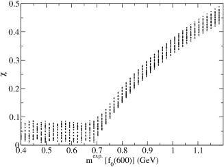
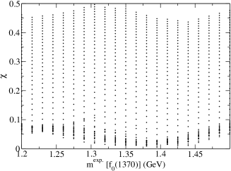
Figure 2: Projection of $\chi$ onto the $\chi-m^{\rm exp.}[f_{0}(600)]$ plane, and onto the $\chi-m^{\rm exp.}[f_{0}(1370)]$ plane. The left figure shows that values of $m^{\rm exp.}[f_{0}(600)]>$ 700 MeV result in a significant disagreement between theory and experiment. The right figure shows that $m^{\rm exp.}[f_{0}(1370)]$ outside of the range 1300-1450 MeV is not favored by the model.

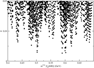
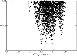
Figure 3: Projection of $\chi$ onto the $\chi-m^{\rm exp.}[f_{0}(600)]$ plane, and onto the $\chi-m^{\rm exp.}[f_{0}(1370)]$ plane. The left figure shows a series of local minima in $\chi$ with the lowest values in the range 500 MeV $\leq m^{\rm exp.}[f_{0}(600)]\leq$ 600 MeV. The right figure shows that the present model predicts that $m^{\rm exp.}[f_{0}(1370)]$ is confined within a smaller range of 1300 MeV to 1450 MeV.

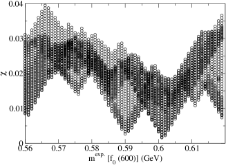
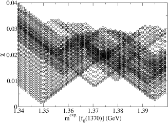
Figure 4: Projection of $\chi$ onto the $\chi-m^{\rm exp.}[f_{0}(600)]$ plane, and onto the $\chi-m^{\rm exp.}[f_{0}(1370)]$ plane. $\chi$ exhibits a series of local minima.

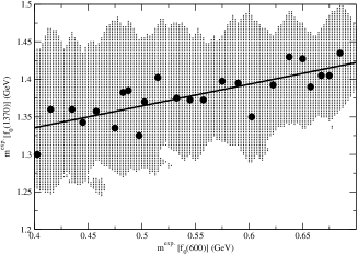
Figure 5: Projection of $\chi$ onto the $m^{\rm exp.}[f_{0}(600)]$$-$$m^{\rm exp.}[f_{0}(1370)]$ plane. In the gray region there is an overall disagreement of less than 5% between theory and experiment. The circles represent points on this plane at which $\chi$ has a local minimum and $\chi<0.02$. The solid line captures the trend of these local minima with equation: $m[f_{0}(1370)]=0.29\,m[f_{0}(600)]+1.22$ GeV.

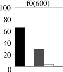
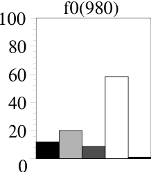
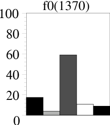
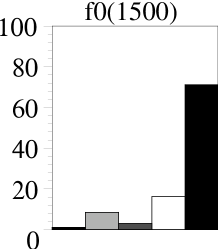
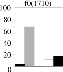
Figure 6: Percentage of the quark and glueball components of the scalar states for values of $m[f_{0}(600)]$ = 558 MeV and $m[f_{0}(1370)]$ = 1373 MeV. In each figure, the columns from left to right respectively represent the percentage of: ${\bar{u}}{\bar{d}}ud$ (black), $({\bar{s}}{\bar{d}}ds+{\bar{s}}{\bar{u}}us)/\sqrt{2}$ (light gray), ${\bar{s}}s$ (dark gray), $({\bar{u}}u+{\bar{d}}d)/\sqrt{2}$ (white), and glueball (black).

More refined numerical analysis narrows down the favored regions to the ranges shown in Fig. 3. We see that the lowest value of $\chi$ occurs within the ranges:

$$m^{\rm exp.}[f_{0}(600)] = 500\rightarrow 600\,{\rm MeV}$$

$$m^{\rm exp.}[f_{0}(1370)] = 1350\rightarrow 1400\,{\rm MeV}$$ (18)

In this region, $\chi$ exhibits a series of local minima, also shown in a more refined numerical work in Fig. 4. Although $\chi$ has its lowest values in the regions given in (18) we see that it only increases by approximately 0.01 outside of this region and can be comparable to the theoretical uncertainties of this framework. Therefore, for a more conservative estimate we take into account all local minima with $\chi<0.02$. This confines the experimental masses to the ranges:

$$m^{\rm exp.}[f_{0}(600)] = 400\rightarrow 700\,{\rm MeV}$$

$$m^{\rm exp.}[f_{0}(1370)] = 1300\rightarrow 1450\,{\rm MeV}$$ (19)

The local minima of $\chi$ in this range are shown in Fig. 5 in which the projection of $\chi$ onto the $m^{\rm exp.}[f_{0}(600)]$$-$$m^{\rm exp.}[f_{0}(1370)]$ plane is given. In the gray region, there is an overall disagreement of less than 5% between theory and experiment. The local minima (with $\chi<0.02$) are shown with dots, together with a linear fit that shows the correlation between the mass of the $f_{0}(600)$ and the $f_{0}(1370)$:

$$m[f_{0}(1370)]=0.29\,m[f_{0}(600)]+1.22\,\,{\rm GeV}$$ (20)

At all local minima (with $\chi<0.02$), a detailed numerical analysis is performed and the eight Lagrangian parameters are determined. The large uncertainties on $m[f_{0}(600)]$ and $m[f_{0}(1370)]$ do not allow an accurate determination of these parameters. In this work we study the correlation between these uncertainties and determination of the Lagrangian parameters. For orientation, let us first begin by investigating the central values of

$$m^{\rm exp.}[f_{0}(600)] = 558\,\,{\rm MeV}$$

$$m^{\rm exp.}[f_{0}(1370)] = 1373\,\,{\rm MeV}$$ (21)

It is important to also notice that the central value of $m[f_{0}(600)]$ = 558 MeV is exactly what was first found in San in applying the nonlinear chiral Lagrangian of this work to $\pi\pi$ scattering. At the particular point of (21), the result of the fit is given in Table 1, and is consistent with the initial investigation of this model in ref. 04_F1 in which the effect of the mixing parameter $\rho$ is only studied at several discrete points. The result given in Table 1 supplements the work of 04_F1 by treating $\rho$ as a general free parameter. The rotation matrix is

$$K^{-1}=\left[\begin{array}[]{ccccc}0.812&-0.065&-0.542&-0.183&0.101\\ 0.346&-0.447&0.294&0.764&-0.106\\ 0.418&0.198&0.768&-0.328&0.299\\ -0.106&0.292&-0.174&0.403&0.844\\ 0.190&0.820&-0.006&0.338&-0.422\end{array}\right]$$ (22)

and in turn determines the quark and glueball components of each physical state as presented in Fig. 6. Several general observations can be made in Fig. 6. Clearly, the $f_{0}(600)$ is dominantly a non-strange four-quark state with a substantial ${\bar{s}}s$ component. On the other hand the dominant structure of the $f_{0}(1370)$ seems to be the reverse of the $f_{0}(600)$. The $f_{0}(980)$ seems to have a dominant non-strange two-quark component with a significant strange four-quark component. The $f_{0}(1500)$ appears to have a dominant glueball component with some minor two and four quark admixtures. The dominant component of the $f_{0}(1710)$ seems to be a strange four-quark state followed by a glueball component.

Lagrangian Parameters	Fitted Values (GeV2)
$c$	2.32 $\times 10^{-1}$
$d$	$-9.11\times 10^{-3}$
$c^{\prime}$	$-4.29\times 10^{-3}$
$d^{\prime}$	$-1.25\times 10^{-2}$
$g$	1.16
$\rho$	$2.87\times 10^{-2}$
$e$	$-2.13\times 10^{-1}$
$f$	$6.10\times 10^{-2}$

Table 1: Fitted values of the Lagrangian parameters for $m[f_{0}(600)]$ = 558 MeV and $m[f_{0}(1370)]$ = 1373 MeV.

The scalar glueball mass can be calculated from the fit in Table 1:

$$m_{G}=\sqrt{2\,\,g}=1.52\,\,{\rm GeV}\\$$ (23)

which is in a range expected from Lattice QCD Lattice .

Next we will examine the effect of deviation from the central values of $m[f_{0}(600)]$ and $m[f_{0}(1370)]$ on the predictions given in Fig. 6. We will find that the average properties of the $f_{0}(600)$, $f_{0}(980)$ and $f_{0}(1370)$ remain close to those given in Fig. 6, but some of the properties of the $f_{0}(1500)$ and $f_{0}(1710)$ are sensitive to such deviations.

To investigate the effect of the mass uncertainties of the $f_{0}(600)$ and $f_{0}(1370)$, we perform 8-parameter fits at each of the local minima of Fig. 5, and determine the variation of the Lagrangian parameters around the values in Table 1. The results are summarized in Table 2. We see that practically the Lagrangian parameters are quite sensitive to the mass of the $f_{0}(600)$ and $f_{0}(1370)$. The only exception is parameter $g$ which determines the glueball mass:

$$m_{G}=\sqrt{2\,\,g}=1.5\rightarrow 1.7\,\,{\rm GeV}$$ (24)

Lagrangian Parameters	Average (GeV2)	Variation (GeV2)
$c$	$1.71\times 10^{-1}$	($0.37\rightarrow 2.60)\times 10^{-1}$
$d$	$-7.32\times 10^{-3}$	($-14.44\rightarrow-2.63)\times 10^{-3}$
$c^{\prime}$	$-2.87\times 10^{-3}$	($-5.32\rightarrow-0.64)\times 10^{-3}$
$d^{\prime}$	$-0.97\times 10^{-2}$	($-1.41\rightarrow-0.27)\times 10^{-2}$
$g$	1.24	1.15 $\rightarrow$ 1.44
$\rho$	$4.7\times 10^{-2}$	($1.31\rightarrow 9.14)\times 10^{-2}$
$e$	$-2.10\times 10^{-1}$	($-3.02\rightarrow-1.76)\times 10^{-1}$
$f$	$3.74\times 10^{-2}$	($1.15\rightarrow 11.40)\times 10^{-2}$

Table 2: The effect of the uncertainties of $m^{\rm exp.}[f_{0}(600)]$ and $m^{\rm exp.}[f_{0}(1370)]$ on the Lagrangian parameters. The averaged value of the parameters (second column) is compared with their (asymmetric) range of variation (third column). Only parameter $g$ (which determines the glueball mass) is relatively insensitive to $m^{\rm exp.}[f_{0}(600)]$ and $m^{\rm exp.}[f_{0}(1370)]$.

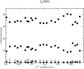
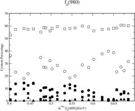
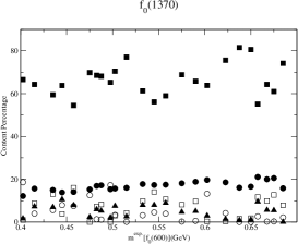
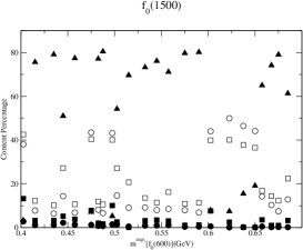
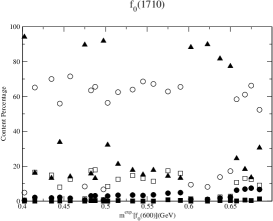
Figure 7: Percentage of quark and glueball components of the scalar states vs $m^{\rm exp.}[f_{0}(600)]$: ${\bar{u}}{\bar{d}}ud$ (filled circles), $({\bar{s}}{\bar{d}}ds+{\bar{s}}{\bar{u}}us)/\sqrt{2}$ (empty circles), ${\bar{s}}s$ (filled squares), $({\bar{u}}u+{\bar{d}}d)/\sqrt{2}$ (empty squares), and glueball (filled triangles).

At the local minima of Fig. 5, we compute the rotation matrix $K^{-1}$ (defined in Eq. (13)) which maps the quark and glueball bases to the physical bases. The results show that $K^{-1}$ is less sensitive to the mass of the $f_{0}(600)$ and $f_{0}(1370)$. For each scalar state, the quark and glueball components versus $m^{\rm exp.}[f_{0}(600)]$ are given in Fig. 7, and the averaged components together with their variations are given in Fig. 8. Although the $m^{\rm exp.}[f_{0}(600)]$ is still over a wide range of 400 to 700 MeV, we see in Fig. 7 that some of the components of the physical state are qualitatively stable: The admixtures of $f_{0}(600)$, $f_{0}(980)$ and $f_{0}(1370)$, as well as some of the components of the $f_{0}(1500)$ and $f_{0}(1710)$ are within a relatively small range of variation. We see that the $f_{0}(600)$ has a dominant ${\bar{u}}{\bar{d}}ud$ component and some ${\bar{s}}s$ content, and has almost the reverse structure of the $f_{0}(1370)$; the $f_{0}(980)$ is dominantly a two quark non-strange state $({\bar{u}}u+{\bar{d}}d)$ with a significant strange four-quark content $({\bar{s}}{\bar{d}}ds+{\bar{s}}{\bar{u}}us)$. Although sensitive to the mass of the $f_{0}(600)$ and $f_{0}(1370)$, we see that the $f_{0}(1500)$ contains a dominant glueball content with some strange four-quark and non-strange two-qurak admixtures; and the $f_{0}(1710)$ is a dominant strange four-quark state with a comparable glueball component.

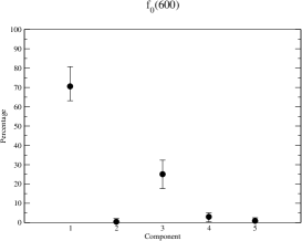
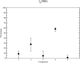
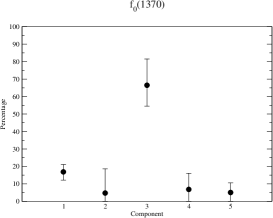
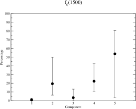
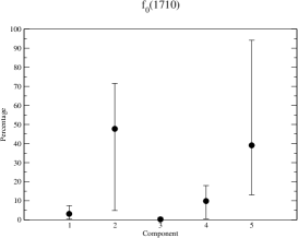
Figure 8: The effects of the mass uncertainties of the $f_{0}(600)$ and $f_{0}(1370)$ on the percentage of the quark and glueball components of the scalar states. Components 1 to 5 respectively represent ${\bar{u}}{\bar{d}}ud$, $({\bar{s}}{\bar{d}}ds+{\bar{s}}{\bar{u}}us)/\sqrt{2}$, ${\bar{s}}s$, $({\bar{u}}u+{\bar{d}}d)/\sqrt{2}$, and glueball. The dots represent the averaged values of each component and the error bars reflect the uncertainties of $m^{\exp.}[f_{0}(600)]$ and $m^{\rm exp.}[f_{0}(1370)]$. The figures show that the components of the $f_{0}(600)$, $f_{0}(980)$ and $f_{0}(1370)$ are not very sensitive to these experimental uncertainties, but some of the components of the $f_{0}(1500)$ and $f_{0}(1710)$ (such as their glueball component) are significantly affected by such uncertainties.

IV Summary and Conclusion

We studied the $I=0$ scalar mesons below 2 GeV using a nonlinear chiral Lagrangian which is constrained by the mass and the decay properties of the $I=1/2$ and $I=1$ scalar meson below 2 GeV [$K_{0}^{*}(800)$, $K_{0}^{*}(1430)$, $a_{0}(980)$ and $a_{0}(1450)$]. This framework provides an efficient approach for predicting the quark and glueball content of the scalar mesons. The main obstacle for a complete prediction is the lack an accurate experimental input for the mass of $f_{0}(600)$ and $f_{0}(1370)$. Nevertheless, we showed that several relatively robust conclusions can be made. We showed that the $f_{0}(600)$, the $f_{0}(980)$ and the $f_{0}(1370)$ have a substantial admixture of two and four-quark components with a negligible glueball component. The present model predicts that the $f_{0}(600)$ is dominantly a non-strange four-quark state; the $f_{0}(980)$ has a dominant non-strange two-quark component; and the $f_{0}(1370)$ has significant ${\bar{s}}s$ admixture. We also showed that this model predicts that the $f_{0}(1500)$ and the $f_{0}(1710)$ have a considerable two and four quark admixtures, together with a dominant glueball component. The current large uncertainties on the mass of $f_{0}(600)$ and $f_{0}(1370)$ do not allow an exact determination of the glueball components of the $f_{0}(1500)$ and the $f_{0}(1710)$, but it is qualitatively clear that the glueball components of these two states are quite large. In addition the present model predicts that the glueball mass is in the range 1.5$-$1.7 GeV (Eq.(24)).

The main theoretical improvement of the model involves inclusion of higher order mixing terms among nonets $N$ and $N^{\prime}$ and the scalar glueball:

$${\rm Tr}\left({\cal M}NN^{\prime}\right)+{\rm Tr}\left({\cal M}N^{\prime}N\right)\hskip 8.5359pt,\hskip 8.5359pt{\rm Tr}({\cal M}N){\rm Tr}(N^{\prime})\hskip 8.5359pt,\hskip 8.5359pt{\rm Tr}({\cal M}N^{\prime}){\rm Tr}(N)\hskip 8.5359pt,\hskip 8.5359pte^{\prime}G{\rm Tr}\left({\cal M}N\right)\hskip 8.5359pt,\hskip 8.5359ptf^{\prime}G{\rm Tr}\left({\cal M}N^{\prime}\right)$$ (25)

However, these terms both mix the quarks and glueballs as well as break SU(3) symmetry, and therefore are of a more complex nature compared to the terms used in this investigation (Eqs. (6) and (9)). Investigation of such higher order mixing terms will be left for future works. It is also important to note that the results presented here are not sensitive to the choice of $\gamma$ which determines the mixing among the $I=1/2$ and $I=1$ mixings in Eq. (6). This is shown in Fig. 9 in which the components of all $I=0$ states are plotted versus $\gamma^{2}$ and show that they are relatively stable. Also in Fig. 10 the bare masses are plotted versus $\gamma^{2}$ in which we see that the expected ordering (i.e. the lowest-lying four-quark nonet $N$ underlies a heavier two-quark nonet $N^{\prime}$ and a glueball) which is examined in ref. Mec using the properties of the $I=1/2$ and $I=1$ scalar states, is not sensitive to the choice of mixing parameter $\gamma$, providing further support for the plausibility of the leading mixing terms considered in the present investigation.

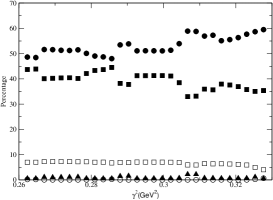
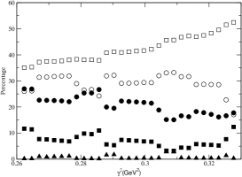
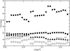
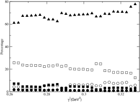
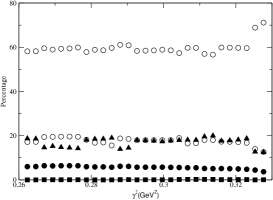
Figure 9: Percentage of quark and glueball components of the scalar states vs $\gamma^{2}$: ${\bar{u}}{\bar{d}}ud$ (filled circles), $({\bar{s}}{\bar{d}}ds+{\bar{s}}{\bar{u}}us)/\sqrt{2}$ (empty circles), ${\bar{s}}s$ (filled squares), $({\bar{u}}u+{\bar{d}}d)/\sqrt{2}$ (empty squares), and glueball (filled triangles). The figures show that the components are not very sensitive to the mixing parameter $\gamma$.

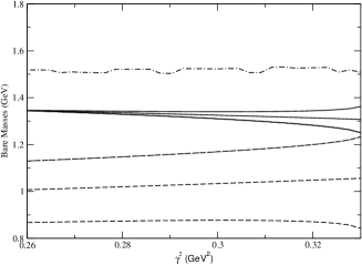
Figure 10: Dependence of the bare masses on $\gamma^{2}$. The four-quark scalar nonet (dashed lines) lies below the quark-antiquark scalar nonet (solid lines) and a scalar glueball (dotted-dashed line).

References

- (1) Particle Data Group, Phys. Lett. B 592 1 (2004).
- (2) R.L. Jaffe, Phys. Rev. D 15, 267 (1977).
- (3) J. Weinstein and N. Isgur, Phys. Rev. D 41, 2236 (1990).
- (4) N.A. Törnqvist, Z. Phys. C 68, 647 (1995); E. van Beveren et al, Z. Phys. C 30, 615 (1986).
- (5) F.Sannino and J. Schechter, Phys. Rev. D 52, 96 (1995); M. Harada, F. Sannino and J. Schechter, Phys. Rev. D 54, 1991 (1996); Phys . Rev. Lett. 78, 1603 (1997).
- (6) D. Black, A.H. Fariborz, F. Sannino and J. Schechter, Phys. Rev. D 58, 054012 (1998).
- (7) D. Black, A.H. Fariborz, F. Sannino and J. Schechter, Phys. Rev. D 59, 074026 (1999).
- (8) A.H. Fariborz and J. Schechter, Phys. Rev. D 60, 034002 (1999).
- (9) D. Black, A.H. Fariborz and J. Schechter, Phys. Rev. D 61, 074030 (2000).
- (10) D. Black, A.H. Fariborz and J. Schechter, Phys. Rev. D 61, 074001 (2000).
- (11) D. Black, A.H. Fariborz, S. Moussa, S. Nasri and J. Schechter, Phys. Rev. D 64, 014031 (2001).
- (12) D. Black, M. Harada and J. Shechter, Phys. Rev. Lett. 88, 181603 (2002); Phys. Rev. D 73,054017 (2006).
- (13) A. Abdel-Rahim, D. Black, A.H. Fariborz, S. Nasri and J. Schechter, Phys. Rev. D 68, 013008 (2003).
- (14) A. Abdel-Rahim, D. Black, A.H. Fariborz, J. Schechter, Phys. Rev. D 67, 054001 (2003).
- (15) A. H. Fariborz, Int. J. Mod. Phys. A 19, 2095 (2004).
- (16) A. H. Fariborz, Int. J. Mod. Phys. A 19, 5417 (2004).
- (17) A.H. Fariborz, R. Jora and J. Schechter, Phys. Rev. D 72, 034001 (2005).
- (18) V. Elias, A.H. Fariborz, Fang Shi and T.G. Steele, Nucl. Phys. A 633, 279 (1998); Fang Shi, T.G. Steele, V. Elias, K.B. Sprague, Ying Xue and A.H. Fariborz, Nucl. Phys. A 671, 416 (2000).
- (19) F.E. Close and A. Kirk, Phys. Lett. B 483, 345 (2000).
- (20) F. Close and N. Tornqvist, J. Phys. G. 28, 249 (2002).
- (21) T. Teshima, I. Kitamura and N. Morisita, J. Phys. G. 28, 1391 (2002).
- (22) T. Teshima, I. Kitamura and N. Morisita, J. Phys. G. 30, 663 (2004).
- (23) M. Napsuciale and S. Rodriguez, Phys. Rev. D 70, 094043 (2004).
- (24) F. Giacosa, T. Gutsche, A. Faessler, Phys. Rev. C 71, 025202 (2005).
- (25) F. Giacosa, Th. Gutsche, V.E. Lyubovitskij, A. Faessler, Phys. Lett. B 622, 277 (2005).
- (26) J. Vijande, A. Valcarce, F. Fernandez, B. Silvestre-Brac, Phys. Rev. D 72, 034025 (2005).
- (27) T.V. Brito, F.S. Navarra, M. Nielsen, M.E. Bracco, Phys. Lett. B 608, 69 (2005).
- (28) S. Narison, hep-ph/0512256.
- (29) L. Maiani, F. Piccinini, A.D. Polosa, V. Riquer, hep-ph/0604018.
-
(30)
N. Ishii, H. Suganuma and H. Matsufuru, Phys. Rev. D66, 014507
(2002);
Xi-Yan Fang, Ping Hui, Qi-Zhou Chen and D. Schutte, Phys. Rev. D65, 114505 (2002);
C.J. Morningstar and M. Peardon, Phys. Rev. D60, 034509 (1999).
J. Sexton, A. Vaccarino and D. Weingarten, Phy. Rev. Lett. 75, 4563 (1995);
G. Bali et al., Phys. Lett. B309, 378 (1993).