A numerical approach to the double real radiation part of $e^{+}e^{-}\to 3$ jets at NNLO

Abstract

We report on the sector decomposition approach to the double real emission part of $e^{+}e^{-}\to 3$ jets at NNLO.

1 INTRODUCTION

Precision measurements at high energy colliders in the recent past led to stringent tests of the Standard Model and important bounds on New Physics. Measurements of jet rates and shape observables in $e^{+}e^{-}$ annihilation are of particular importance, as they allow for a precise determination of the strong coupling constant $\alpha_{s}$. At hadron colliders, a cross section involving $n$ jets is proportional to $\alpha_{s}^{n}$ at leading order, such that an accurate knowledge of $\alpha_{s}$ will be important at the LHC, where many interesting processes contain jets in the final state.

A determination of $\alpha_{s}$ from jet rates and shape observables is described e.g. in [1], where one can see that for LEP measurements, the experimental uncertainty is smaller than the theoretical one, which is based on resummed next-to-leading order (NLO) calculations. As the theoretical error is dominated by scale uncertainties, an NNLO calculation will considerably improve this situation. A future International Linear Collider will allow for precision measurements at the per-mille level, which offer the possibility of a determination of $\alpha_{s}$ with unprecedented accuracy, provided that theoretical predictions at NNLO are available.

2 COMPUTATIONAL METHODS

The calculation of $e^{+}e^{-}\to 3$ jets at order $\alpha_{s}^{3}$ requires the calculation of virtual two-loop corrections combined with a $1\to 3$ parton phase space, one-loop corrections combined with a $1\to 4$ parton phase space where one parton can become soft and/or collinear (“unresolved”), and the tree level matrix element squared for $1\to 5$ partons where up to two partons can become unresolved. The unresolved particles lead to a complicated infrared singularity structure which manifests itself in $1/\epsilon$ poles upon phase space integration. These singularities have to be subtracted and cancelled with the ones from the virtual contributions before a Monte Carlo program can be constructed. To achieve this task, two different approaches have been followed, one relying on the manual construction of an analytical subtraction scheme [2, 3, 4, 5, 6, 7, 8], the other one relying on sector decomposition [9, 10, 11, 12, 13, 14, 15, 16, 17, 18, 19, 20, 21]. The main features of the methods based on the explicit construction of a subtraction scheme are the following: The subtraction terms are integrated analytically over the unresolved phase space, such that the pole coefficients are obtained in analytic form. This requires appropriate phase space factorisation and subtraction terms which are simple enough to be integrated analytically in $D=4-2\epsilon$ dimensions. This method naturally leads to a close to minimal number of subtraction terms, and allows insights into the infrared structure of QCD.

In the sector decomposition approach, the poles are isolated by an automated algebraic procedure acting in parameter space, and the pole coefficients are integrated numerically. The advantages of this approach reside in the fact that the extraction of the infrared poles is done by the computer, and that the subtraction terms can be very complicated as they are integrated only numerically. On the other hand, the algorithm which isolates the poles increases the number of original functions, thus producing rather large expressions.

The application of sector decomposition to real radiation at NNLO first has been presented in [12, 13], and the combination of the sector decomposition approach with a measurement function first has been proposed in [14]. A number of NNLO results based on this method have been obtained meanwhile [13, 14, 15, 16, 17, 18, 19, 20]. Its application to the double real radiation part of $e^{+}e^{-}\to 3$ jets at order $\alpha_{s}^{3}$ [21] is particularly challenging due to the high number of massless particles in the final state, which leads to a very complicated infrared singularity structure.

3 SECTOR DECOMPOSITION

The wide range of applicability of sector decomposition goes back to the fact that it acts in parameter space by a simple mechanism. The parameters can be Feynman parameters in the case of multi-loop integrals, or phase space integration variables, or a combination of both. In the following, the working mechanism of sector decomposition will be outlined only briefly for the example of phase space integrals, details can be found in [11, 15, 18, 21].

The phase space integral of a matrix element squared, combined with some measurement function ${\cal J}$ defining a physical observable, typically contains “overlapping” structures like

$$\int{\rm d}s_{13}\,{\rm d}s_{23}\,\,s_{13}^{-1-\epsilon}\,\,\frac{{\cal J}(s_{13},s_{23})}{s_{13}+s_{23}}$$

$$\sim \int_{0}^{1}dx\,dy\,x^{-1-\epsilon}\,\frac{{\cal J}(x,y)}{x+y}\;,$$

where only the dependence on two of the integration variables is shown for pedagogical simplicity. In order to extract the poles in $1/\epsilon$, the singularities for $x,y\to 0$ need to be factorised. Sector decomposition is a way to achieve the factorisation of this type of entangled singularities in an algorithmic way: First the integration region is split into sectors where the variables $x$ and $y$ are ordered by multiplying with unity in the form $[\underbrace{\Theta(x-y)}_{(a)}+\underbrace{\Theta(y-x)}_{(b)}]$. Then the integration domain is remapped to the unit cube: after the substitutions $y=x\,t$ in sector (a) and $x=y\,t$ in sector (b), one has

$$I = \int_{0}^{1}dx\,x^{-1-\epsilon}\int_{0}^{1}dt\,(1+t)^{-1}{\cal J}(x,x\,t)$$

$$+ \int_{0}^{1}dy\,y^{-1-\epsilon}\int_{0}^{1}dt\,t^{-1-\epsilon}\,(1+t)^{-1}{\cal J}(y\,t,y)$$

where the singularities are now factorised. For more complicated functions, several iterations of this procedure may be necessary, but it is easily implemented into an automated subroutine. Once all singularities are factored out, they can be subtracted using identities like

$$\int_{0}^{1}dx\int_{0}^{1}dy\,x^{-1-\kappa\epsilon}f(x,y)=$$

$$-\frac{1}{\kappa\epsilon}\,\int_{0}^{1}dy\,f(0,y)$$

$$+\int_{0}^{1}dx\int_{0}^{1}dy\,x^{-\kappa\epsilon}\,\frac{f(x,y)-f(0,y)}{x}\;,$$

where we recognise the form of plus distributions. The result can subsequently be expanded in $\epsilon$, such that a Laurent series in $\epsilon$ is obtained, where the pole coefficients are sums of finite parameter integrals which can be evaluated numerically.

For the numerical evaluation it has to be assured that no integrable singularities are crossed which spoil the numerical convergence. In the double real radiation part of $e^{+}e^{-}\to 3$ jets, singularities which are located in the interior of the integration region do indeed occur. However, it is always possible to remap them to endpoint singularites by a convenient variable transformation. After such a remapping, they are amenable to sector decomposition.

4 APPLICATION TO $e^{+}e^{-}\to 3$ JETS AT NNLO

In order to calculate the double real radiation part of $e^{+}e^{-}\to 3$ jets at NNLO, sector decomposition is applied to extract the poles appearing in massless $1\to 5$ particle integrals. As a simple example, let us consider the 5-particle cut of the ladder graph shown in fig. 1.

Sector decomposition leads to [21]

$$T_{1\to 5} = -C_{F}^{3}\left(\frac{\alpha_{s}}{4\pi}\right)^{3}\,T_{1\to 2}\left\{\frac{0.16662}{\epsilon^{3}}\right.$$ (3)

$$\left.+\frac{1}{\epsilon^{2}}\,[1.4993-0.4999\,\log{\left(\frac{q^{2}}{\mu^{2}}\right)}]\right.$$

$$\left.+\frac{1}{\epsilon}\,[5.5959-4.4978\,\log{\left(\frac{q^{2}}{\mu^{2}}\right)}\right.$$

$$+\left.0.7498\,\log^{2}{\left(\frac{q^{2}}{\mu^{2}}\right)}]\,+\,\mbox{finite}\right\}\;,$$

where the numerical accuracy is better than 1%. The correctness of the result can be checked by exploiting the fact that the sum over all cuts of a given (UV renormalised) diagram must be infrared finite. This is shown diagrammatically in fig. 2. After UV renormalisation, we obtain the condition

$$T_{1\to 5}+z_{1}\,T_{1\to 4}+z_{2}\,T_{1\to 3}+z_{3}\,T_{1\to 2}=\mbox{finite}\;,$$ (4)

where $T_{1\to i}$ denotes the diagram with $i$ cut lines.

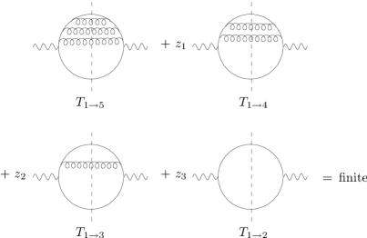
Figure 2: Cancellation of IR divergences in the sum over all cuts of the renormalised graph

The renormalisation constants $z_{i}$ (in Feynman gauge) are given by [15, 21]

$$z_{1} = C_{F}\frac{\alpha_{s}}{4\pi}\,\frac{1}{\epsilon}\,,\,z_{2}=C_{F}^{2}\left(\frac{\alpha_{s}}{4\pi}\right)^{2}\,\left(\frac{1}{2\epsilon^{2}}-\frac{1}{4\epsilon}\right)$$

$$z_{3} = C_{F}^{3}\left(\frac{\alpha_{s}}{4\pi}\right)^{3}\,\left(\frac{1}{6\epsilon^{3}}-\frac{1}{4\epsilon^{2}}+\frac{1}{6\epsilon}\right)\;.$$ (5)

The expressions in eq. (4) for $i<5$ combine to

$$z_{1}\,T_{1\to 4}+z_{2}\,T_{1\to 3}+z_{3}\,T_{1\to 2}=$$

$$C_{F}^{3}\left(\frac{\alpha_{s}}{4\pi}\right)^{3}\,T_{1\to 2}\left\{\frac{1}{6\epsilon^{3}}+\frac{1}{2\epsilon^{2}}\,[3-\log{\left(\frac{q^{2}}{\mu^{2}}\right)}]\right.$$

$$+\frac{1}{\epsilon}\,[5.61-\frac{9}{2}\log{\left(\frac{q^{2}}{\mu^{2}}\right)}+\frac{3}{4}\log^{2}{\left(\frac{q^{2}}{\mu^{2}}\right)}]$$

$$+\left.\,\mbox{finite}\right\}\;.$$ (6)

We can see that the poles in (6) are exactly cancelled by the 5-parton contribution (3) within the numerical precision.

4.1 Differential results

Although the sector decomposition approach is considered to be a “numerical method”, as the pole coefficients are only calculated numerically, the isolation of the poles is an algebraic procedure, leading to a set of finite functions for each pole coefficient as well as for the finite part. These finite functions are written to a Fortran program and evaluated numerically using Monte Carlo techniques. In order to obtain results which are differential in a certain physical observable, any (infrared safe) measurement function can be included at the level of the final Monte Carlo program, which means that the subtractions and expansions in $\epsilon$ do not have to be redone each time a different observable is considered. Further, the measurement function does not have to be an analytic function, but can be a subroutine acting on the four-momenta of the final state particles, as it is typically the case for a jet clustering routine. The reason why such a maximal flexibility is possible resides in the fact that the program described in [21] has the architecture of a partonic event generator. This requires to keep track of the mappings of the original phase space variables to the variables used in each sector, i.e. each endpoint of the iterated decompsition tree. These mappings will be different for each sector (cf. the arguments of the function ${\cal J}$ in the first and second line of eq. (3)), but keeping this information allows to express the energies and angles of the final state particles in terms of the sector variables and thus to reconstruct the fully differential information on the final state. In this procedure, function evaluations in sectors which do not pass the kinematical requirements imposed by the measurement function are unavoidable. Having to deal with a large number of sectors, this can lead to a serious drop in efficiency of the Monte Carlo program. Therefore, in order to construct a program which produces results within a reasonable time scale, it is crucial to keep the number of sectors low. This can be achieved by (a) using optimised phase space parametrisations for each topology, (b) using information on physical limits in the decomposition algorithm.

Optimising the phase space parametrisations means the following: The matrix element squared can be divided into a certain number of topologies, which are defined by a certain set of denominators (which will be combinations of Mandelstam invariants, see e.g. eq. (3)). In a given phase space parametrisation, some of the invariants will naturally be in a factorised form, but such a form cannot be achieved for all invariants simultaneously. An optimised parametrisation is one where the number of non-factorising invariants in the denominator is kept minimal. Therefore one has to choose different parametrisations for each topology, resp. for each class of topologies with the same factorisation properties.

Using information on physical limits exploits the fact that in most cases of physical relevance, the measurement function is such that it would prevent certain poles from arising at all if it were included in the $\epsilon$-expansion. For example, poles associated with a 2-jet configuration, where 3 of the 5 final state particles become theoretically unresolved, will be killed by a 3-jet measurement function. It would therefore be desirable to suppress the terms associated with such configurations already at the level of the $\epsilon$-expansion, in order to avoid an unnecessarily large number of terms associated with the isolation of these poles. On the other hand, we would like to keep the flexibility to include any measurement function only at the stage of the final Monte Carlo program. Focusing on the process $e^{+}e^{-}\to 3$ jets, this dilemma has been solved by including some “preselection rules” in the $\epsilon$-expansion which reject configurations which will surely be 2-jet configurations. In the example shown here, this can be achieved by introducing a cut parameter $y^{\rm th}$ – which must be smaller than any possible experimental resolution parameter $y^{\rm cut}$ – for the variable $s_{1345}$, as $s_{1345}\to 0$ always corresponds to a 2-jet configuration. In this way, one can reduce the size of the expressions considerably without loosing the flexibility to specify different jet algorithms later.

To illustrate the action of the jet function, 3–, 4– and 5–jet rates using the JADE algorithm [22] are shown in Fig. 3, based on the toy matrix element built from the graphs shown in Fig. 2.

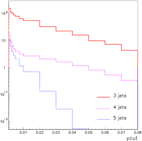
Figure 3: 3–, 4– and 5–jet rates at order $\alpha_{s}^{3}$ for the toy matrix element

As a more complex example, the double real radiation part of a non-planar topology (see fig. 4) also has been calculated.

In this case, square-root terms in the denominator are unavoidable, which implies that the expressions produced by the sector decomposition will be larger due to the presence of more non-factorising denominators. The virtual corrections to this topology have not yet been included.

Note that the results shown in figs. 3 and 4 are unphysical, as they do not contain all contributions to form a gauge invariant quantity. The purpose of these figures is merely to demonstrate the action of the jet function and thus the power of the method to produce differential results.

The CPU time is ${\cal O}(2h)$ for a precision better than 1%. Note that all topologies can be calculated in parallel, such that the CPU time for the full double real radiation part will be of the order of the one needed for the most complicated topology.

What remains to be done, besides the inclusion of the remaining topologies, is the combination with the one-loop plus single real and the two-loop virtual corrections. How to proceed efficiently by combining sector decomposition with analytical results is sketched in [17, 23].

5 SUMMARY AND OUTLOOK

The method based on sector decomposition to calculate $e^{+}e^{-}\to 3$ jets at NNLO has the advantage that the isolation of the infrared poles is done by an automated routine and that it does not require the analytical integration of subtraction terms. However, the method produces large expressions, which is an issue for a process like $e^{+}e^{-}\to 3$ jets at NNLO where the matrix element to start with is already large. It has been described how to limit the proliferation of terms in the course of sector decomposition, and differential results have been shown for a subpart of the process.

The inclusion of massive particles within this method is certainly more straightforward than in analytical approaches. In fact, as the masses act as infrared regulators, the number of decompositions will be less and therefore the produced expressions should be smaller than in massless cases.

References

- [1] S. Bethke, hep-ex/0606035.
- [2] D. A. Kosower, Phys. Rev. D67, 116003 (2003).
- [3] S. Weinzierl, JHEP 03, 062 (2003) and hep-ph/0606008.
- [4] A. Gehrmann-De Ridder, T. Gehrmann, and E. W. N. Glover, Nucl. Phys. B691, 195 (2004).
- [5] W. B. Kilgore, Phys. Rev. D70, 031501 (2004).
- [6] S. Frixione and M. Grazzini, JHEP 06, 010 (2005).
- [7] G. Somogyi, Z. Trocsanyi, and V. Del Duca, JHEP 06, 024 (2005).
- [8] A. Gehrmann-De Ridder, T. Gehrmann, and E. W. N. Glover, JHEP 09, 056 (2005).
- [9] K. Hepp, Commun. Math. Phys. 2, 301 (1966).
- [10] M. Roth and A. Denner, Nucl. Phys. B479, 495 (1996).
- [11] T. Binoth and G. Heinrich, Nucl. Phys. B585, 741 (2000).
- [12] G. Heinrich, Nucl. Phys. Proc. Suppl. 116, 368 (2003).
- [13] A. Gehrmann-De Ridder, T. Gehrmann, and G. Heinrich, Nucl. Phys. B682, 265 (2004).
- [14] C. Anastasiou, K. Melnikov, and F. Petriello, Phys. Rev. D69, 076010 (2004).
- [15] T. Binoth and G. Heinrich, Nucl. Phys. B693, 134 (2004).
- [16] C. Anastasiou, K. Melnikov, and F. Petriello, Phys. Rev. Lett. 93, 032002 (2004).
- [17] G. Heinrich, Nucl. Phys. Proc. Suppl. 135, 290 (2004).
- [18] C. Anastasiou, K. Melnikov, and F. Petriello, Nucl. Phys. B724, 197 (2005).
- [19] C. Anastasiou, K. Melnikov, and F. Petriello, hep-ph/0505069.
- [20] K. Melnikov and F. Petriello, hep-ph/0603182.
- [21] G. Heinrich, hep-ph/0601062.
- [22] JADE collaboration, S. Bethke et al., Phys. Lett. B213, 235 (1988).
- [23] G. Heinrich, Nucl. Phys. Proc. Suppl. 157 (2006) 43.