Fractional Analytic Perturbation Theory in Minkowski space and application to Higgs boson decay into a $b\bar{b}$ pair

Abstract

We work out and discuss the Minkowski version of Fractional Analytic Perturbation Theory (MFAPT) for QCD observables, recently developed and presented by us for the Euclidean region. The original analytic approach to QCD, initiated by Shirkov and Solovtsov, is summarized and relations to other proposals to achieve an analytic strong coupling are pointed out. The developed framework is applied to the Higgs boson decay into a $b\bar{b}$ pair, using recent results for the massless correlator of two quark scalar currents in the $\overline{\text{MS}\vphantom{{}^{1}}}$ scheme. We present calculations for the decay width within MFAPT including those non-power-series contributions that correspond to the ${\cal O}\left(\alpha_{s}^{3}\right)$-terms, taking also into account evolution effects of the running coupling and the $b$-quark-mass renormalization. Comparisons with previous results within standard QCD perturbation theory are performed and the differences are pointed out. The interplay between effects originating from the analyticity requirement and the analytic continuation from the spacelike to the timelike region and those due to the evolution of the heavy-quark mass is addressed, highlighting the differences from the conventional QCD perturbation theory.

I Introduction

QCD perturbation theory in the spacelike (Euclidean) domain is based on a power-series expansion in terms of the running (effective) coupling $\alpha_{s}(Q^{2})$, ($Q^{2}=-q^{2}>0$), which in one-loop order reads

$$\alpha_{s}(Q^{2})=\frac{4\pi}{b_{0}}~{}a(L)=\frac{4\pi}{b_{0}}~{}\frac{1}{L}~{}$$ (1)

with $\displaystyle~{}b_{0}=11-\frac{2}{3}N_{f}$,  $L=\ln(Q^{2}/\Lambda^{2})$, where $\Lambda^{2}\equiv\Lambda_{\text{QCD}}^{2}$, and with the “normalized” coupling $a(L)$ satisfying the renormalization-group equation

$$\frac{da(L)}{dL}=-a^{2}\left(1+c_{1}a+c_{2}a^{2}\ldots\right)\,.$$ (2)

Here $c_{1}=b_{1}/b_{0}^{2}$ and $c_{2}=b_{2}/b_{0}^{3}$ are auxiliary expansion parameters (see Appendix A and also Section III in Ref. BMS05 ). The one-loop solution of this equation suffers from an artificial singularity at $L=0$, called the Landau pole. This prevents the application of perturbative QCD in the low-momentum spacelike regime with the effect that hadronic quantities, calculated at the partonic level in terms of a power-series expansion in the running coupling, are not well defined. Besides, from the theoretical point of view, such ghost singularities contradict causality rendering a spectral Källén–Lehmann representation meaningless. On the other hand, in the timelike, Minkowski, region ($q^{2}>0$) the definition of the running coupling turns out to be difficult. The origin of the problem is that the QCD perturbative expansion cannot be defined in a direct way in this domain.

Many efforts have been made since the early days of QCD to define an appropriate coupling parameter in Minkowski space in order to describe crucial timelike processes like the $e^{+}e^{-}$ annihilation into hadrons, quarkonium and $\tau$-lepton decays into hadrons, etc. Most of these attempts—see, for instance, PR81 ; PRR83 ; Mar88 —were based on the analytic continuation of the strong coupling from the deep Euclidean region, where perturbative QCD calculations are safely performed, to the Minkowski space, where physical measurements are carried out. Over the years, it became clear that in the infrared (IR), the strong coupling may reach a stable fixed point and cease to increase. This behavior would imply that color forces may saturate at this low-momentum scale meaning that gluons decouple from quarks because they “see” them as a whole, i.e., in a quasi colorless configuration. Cornwal Cor82 studied, within a vortex-condensate formalism, the formation of a mass gap, or effective gluon mass, that prevents the strong coupling becoming infinite at the Landau pole. Similar attempts were undertaken by other authors in subsequent years PP79 ; GHN93 ; MS92 using different techniques, but basing their arguments on the gluon acquiring an effective mass that works like an IR regulator in the low-momentum region. It was shown in Ste99 that this version of the IR-protected strong coupling can be related to the Sudakov factor for the non-emission of soft gluons, in the sense that gluons with wavelengths above some characteristic (nonperturbative) length scale, cannot resolve individual quarks because these segregate into a colorless mock-hadron state.

In separate parallel developments, Radyushkin Rad82 , and Krasnikov and Pivovarov KP82 have obtained analytic expressions for the one-loop running coupling (and its powers) directly in Minkowski space using an integral transformation from the spacelike to the timelike regime reverse to that for the Adler $D$-function (for more details, we refer the interested reader to Shi00 ; BRS00 ; Shi01 ). This sort of analytic coupling in the timelike region was rediscovered in the context of the resummation of fermion bubbles by Beneke and Braun BB95 and also by Ball, Beneke, and Braun in BBB95 , the latter work in connection with techniques and applications to the $\tau$ hadronic width.

A systematic approach, termed Analytic Perturbation Theory (APT), has emerged in the last decade from studies initiated by Shirkov and Solovtsov SS96 ; SS97 . The main quantity of this framework is the spectral density with the aid of which an analytic running coupling is defined in the Euclidean region using a spectral representation. The same spectral density can be used to define the running coupling in the timelike region having recourse to the dispersion relation for the Adler function MS97 ; MiSol97 . These integral transformations, called $\hat{R}$ and $\hat{D}$ operations (see next section), coincide with those invented in Rad82 ; KP82 and provide the possibility to define simultaneously an analytic running coupling in both the Euclidean and the Minkowski space. Meanwhile this analytic approach has been extended beyond the one-loop level MiSol97 ; SS98 and important techniques for numerical calculations have been developed Mag99 ; Mag00 ; KM01 ; Mag03u ; KM03 ; Mag05 . The approach has already been applied to the calculation of several hadronic quantities, important examples being the inclusive decay of a $\tau$-lepton into hadrons JS95-349 ; MSS97 ; MSSY00 , the momentum-scale and scheme dependence of the Bjorken MSS98 and the Gross–Llewellyn Smith sum rule MSS98GLS , $\Upsilon$ decays into hadrons SZ05 , etc. Moreover, it has been extended to processes, like the $\gamma^{*}\gamma\to\pi$ transition form factor SSK99 ; SSK00 and the pion’s electromagnetic form factor at the next-to-leading order (NLO) of QCD perturbation theory SSK99 ; SSK00 ; BPSS04 , processes that contain more than a single perturbative scale, accounting also for Sudakov suppression.

Overall, this analytic approach (see for some review SS99 ; Shi00 ; SS06 ) does provide a quite reliable description of hadronic quantities in QCD, though there is also criticism GIZ01 and alternative proposals and views of how to avert singularities in the running coupling Piv91a ; LeDiPi92 ; DMW96 ; Dok98 ; CMNT96 ; Gru97 ; GGK98 ; Magn00 ; BRS00 ; Piv01 ; GKP01 ; Nes03 ; Ale05 ; CV06 ; Rac06 —in particular concerning the deep IR region $Q^{2}\leq\Lambda^{2}$, where eventually the presence of a non-vanishing hadronic mass may become important NP04 . It also suffers severe limitations in concept and application to processes beyond the leading order (LO) of QCD perturbation theory because it assumes that the only quantities that have to be analytic in the complex $Q^{2}$ plane are the running coupling and its integer powers. But it was shown in DR81 ; BT87 ; Mul98 ; MNP99a ; MNP01a ; MMP02 that typical three-point functions, like the electromagnetic or pion-photon transition form factor, at the NLO level of perturbative QCD, and beyond, contain typical logarithms depending on an additional scale that serves as a factorization or evolution scale. These logarithms, though not affecting the Landau singularity, do contribute to the spectral density. This has led Karanikas and Stefanis (KS) KS01 ; Ste02 to extend the concept of analyticity (the dispersion relations) from the level of the coupling and its powers to the level of QCD hadronic amplitudes as a whole. This generalized encompassing version of the analyticity requirement demands that all terms that may contribute to the spectral density, i.e., affect the discontinuity across the cut along the negative real axis $-\infty<Q^{2}<0$, must be included into the “analytization” procedure. The implementation of the KS analyticity postulate entails the extension of the original APT to non-integer (fractional) powers of the running coupling, which, in particular, encompasses the logarithms of the factorization (evolution) scale just mentioned.

In this context it is worth emphasizing that fractional powers of the strong coupling were considered implicitly in BKM01 . The systematic development of the Fractional Analytic Perturbation Theory (FAPT) for QCD in the Euclidean space was recently carried out in BMS05 (see also SBKM06 for a brief introduction) and was applied in BKS05 to the factorized part of the pion’s electromagnetic form factor that epitomizes three-point functions in perturbative QCD. The pivotal advantage of this scheme is the diminished sensitivity of the perturbative result on the factorization scale that parallels the strong renormalization-scheme independence, already established within APT at the NLO level with respect to the same observable, in the exhaustive in-depth analysis of BPSS04 (an abridged version of which is given in SBMPS04 —see also Ste04mon ; AB04pg ; AB04ca ). The aim of the present investigation is to extend this analytic framework to the Minkowski space twining the two regions, spacelike and timelike, for any real index and any argument of the couplings and creating a new calculational paradigm for applications to hadronic observables in QCD perturbation theory. The formal discussion of the main characteristics of FAPT in Minkowski space (for which we use the abbreviation MFAPT) is carried out for two- and three-loop running-coupling parameters, investigating also the convergence properties of this type of expansion. To assess the consequences of MFAPT for observables and elaborate on its advantages in detail, it is best to study a quantity at a high-loop order of perturbation theory. To this end, we consider the correlator of two scalar bottom-quark currents, whose imaginary part $R_{\text{S}}(s)$ is directly proportional to the decay width of a scalar Higgs boson to a bottom-antibottom pair. Considerable progress has been achieved with respect to this quantity during the last few years mainly thanks to the efforts of Chetyrkin and collaborators Che96 ; ChKS97 ; BCK05 . In the present investigation we will provide estimates for $R_{\text{S}}(s)$ within multiloop MFAPT, using exclusively the $\overline{\text{MS}\vphantom{{}^{1}}}$ scheme, and compare them with previous various results within conventional perturbative QCD up to the order ${\cal O}\left(\alpha_{s}^{4}\right)$. The evolution effects due to the running of the strong coupling and the heavy-quark mass will be calculated up to three loops, borrowing the corresponding four-loop expansion coefficient for the Adler function from BCK05 . We emphasize in this context that our investigation is mainly meant to expose the conceptual advantages of the method, rather than to be used as a phenomenological tool for this quantity.

The paper is organized as follows. In Sec. II we provide a mini review of the main features of APT, starting with the Euclidean region and completing the section with a discussion of the Minkowski domain. Though this material is mostly based on previously published works, its presentation here for any real coupling power is new and has not appeared before in the literature. Section III is devoted to the generalization and extension of FAPT BMS05 to timelike momenta, giving rise to MFAPT. In this section we present our main theoretical results and provide the reader with explicit (but approximate) two-loop expressions for the analytic powers of the timelike coupling. Similar formal expressions for any (higher) loop can be derived along these lines, with the three-loop case being outlined in Appendices A, B, and C). We close the discussion by giving analysis of the convergence properties of the perturbative expansion within our analytic scheme. Section IV contains an application of our framework on the correlator of two scalar currents of $b$-quarks and the Higgs boson decay into a bottom–antibottom pair, presenting estimates for the width (actually for the quantity $R_{\text{S}}$) of this process for different orders of the perturbative expansion, as specified above, and comparing our results with those obtained with the standard perturbative QCD expansion. Emphasis is put on the inherent advantage of our method to include into the analytic Minkowski couplings the crucial contributions stemming from the resummed $\pi^{2}$ terms owing to the analytic continuation. Our conclusions are drawn in Sec. V, where we also compile the benchmarks of FAPT in both the Euclidean and the Minkowski region. Important technical details are collected in four appendices.

II Conceptual essentials of Analytic Perturbation Theory

Here we introduce the main theoretical elements of APT, basing our considerations on Shi98 ; SS99 , the aim being to provide a comprehensive mini-review of the subject and equip the reader with all knowledge necessary for the extension to fractional powers in Minkowski space in Sec. III. As mentioned in the Introduction, the initial motivation to invent new couplings was the desire to interrelate the Adler $D$-function,

$$D(Q^{2},\mu^{2})=\sum_{n}d_{n}(Q^{2}/\mu^{2})~{}a^{n}(\mu^{2})\stackrel{{\scriptstyle\mu^{2}=Q^{2}}}{{\longrightarrow}}D(Q^{2})=\sum_{n}~{}d_{n}~{}a^{n}(Q^{2})\,,$$ (3)

calculable in the Euclidean domain, and the quantity $\displaystyle R_{e^{+}e^{-}}=\frac{\sigma(e^{+}e^{-}\to\text{hadrons})}{\sigma(e^{+}e^{-}\to\mu^{+}\mu^{-})}$,

$$R(s,\mu^{2})=\sum_{m}r_{m}(s/\mu^{2})~{}a^{m}(\mu^{2})\stackrel{{\scriptstyle\mu^{2}=s}}{{\longrightarrow}}R(s)=\sum_{m}~{}r_{m}~{}a^{m}(s)\ ,$$ (4)

which is measured in the Minkowski region. Both quantities are considered in standard QCD perturbation theory, demanding that the couplings satisfy the renormalization-group (RG) equation. In minimal-subtraction renormalization schemes the coefficients $d_{n}=d_{n}(1),~{}r_{m}=r_{m}(1)$, entering, respectively, the r.h.s. of Eqs. (3) and (4), are numerical constants. The functions $D$ and $R$ can be related to each other via a dispersion relation without any reference to perturbation theory. However, employing a perturbative expansion on the l.h.s. of Eqs. (3) and (4), one obtains, in fact, a relation between the powers of $\ln(s/\mu^{2})$ and $\ln(Q^{2}/\mu^{2})$ in the coefficients $r_{m}(s/\mu^{2})$ and $d_{n}(Q^{2}/\mu^{2})$, while the powers of $\alpha_{s}(\mu^{2})$ reveal themselves as numerical parameters. Upon setting $\mu^{2}=Q^{2}$ on the r.h.s. of Eq. (3) (or $\mu^{2}=s$ in Eq. (4)), the coefficients $d_{n}$ (analogously $r_{n}$) become constants, whereas the coupling powers $\alpha^{n}_{s}(Q^{2})$ (equivalently, $\alpha^{m}_{s}(s)$) are part of the integral transformations (see below). But, if these coupling parameters are the standard running ones, then this connection fails at any loop order because of the Landau singularity in the Euclidean space. Questions arise whether analytic versions of both types of couplings may exist for which the above expressions could be connected. We shall see in the next step how this goal can, indeed, be achieved using non-power-series (functional) expansions within APT SS97 ; MS97 ; MiSol97 ; Shi98 ; SS99 ; SS06 ; Shi00b ; Shi00 ; Shi01 .

The analytic images of the powers of the normalized running coupling, cf. Eq. (1), in the Euclidean space can be defined by the formal linear operation $\textbf{A}_{\text{E}}$:

$$\textbf{A}_{\text{E}}\left[a^{n}_{(l)}\right] = {\cal A}^{(l)}_{n}\text{~{}~{}~{}with~{}~{}~{}}{\cal A}^{(l)}_{n}(Q^{2})\equiv\int_{0}^{\infty}\!\frac{\rho^{(l)}_{n}(\sigma)}{\sigma+Q^{2}}\,d\sigma\,,$$ (5)

where the spectral density is defined as

$$\rho^{(l)}_{n}(\sigma)\equiv\frac{1}{\pi}\,\textbf{Im}\,\big{[}a^{n}_{(l)}(-\sigma)\big{]}\,.$$ (6)

The power (index) $n$ denotes here only integer values, whereas the loop order is indicated by $l$ in parenthesis. We will show later that these relations are valid also for fractional powers (indices) $\nu$.

Analogously, the analytic images of the normalized running coupling in Minkowski space are defined by means of another linear operation, $\textbf{A}_{\text{M}}$, viz.,

$$\textbf{A}_{\text{M}}\left[a^{n}_{(l)}\right]={\mathfrak{A}}^{(l)}_{n}\text{~{}~{}~{}with~{}~{}~{}}{\mathfrak{A}}^{(l)}_{n}(s)\equiv\int_{s}^{\infty}\!\frac{\rho^{(l)}_{n}(\sigma)}{\sigma}\,d\sigma\,.$$ (7)

These “analytization” operations can be represented by the following two integral transformations:

• $\hat{D}$ from the timelike region to the spacelike region

  $$\hat{D}\big{[}{\mathfrak{A}}^{(l)}_{n}\big{]} = {\cal A}^{(l)}_{n}\text{~{}~{}~{}with~{}~{}~{}}{\cal A}^{(l)}_{n}(Q^{2})\equiv Q^{2}\int_{0}^{\infty}\!\frac{{\mathfrak{A}}^{(l)}_{n}(\sigma)}{\big{(}\sigma+Q^{2}\big{)}^{2}}\,d\sigma$$ (8)

  and

• $\hat{R}$ for the inverse transformation (adopting the terminology of Shirkov, see, for instance, Shi00 ; Shi01 ; Shi05 )

  $$\hat{R}\big{[}{\cal A}^{(l)}_{n}\big{]} = {\mathfrak{A}}^{(l)}_{n}\text{~{}~{}~{}with~{}~{}~{}}{\mathfrak{A}}^{(l)}_{n}(s)\equiv\frac{1}{2\pi i}\int_{-s-i\varepsilon}^{-s+i\varepsilon}\!\frac{{\cal A}^{(l)}_{n}(\sigma)}{\sigma}\,d\sigma\,,$$ (9)

where the last integral is evaluated along the contour shown in Fig. 1.

Figure 1: Integration contour for the $\hat{R}$-operation in Eq. (9).

Note that these operations are connected to each other by the relation

$$\hat{D}\hat{R}=\hat{R}\hat{D}=1\,,$$ (10)

valid for the whole set $\big{\{}{\cal A}_{n},{\mathfrak{A}}_{n}\big{\}}$ and at any loop order.

The operations $\textbf{A}_{\text{E}}$ and $\textbf{A}_{\text{M}}$, which define, respectively, the analytic running couplings in the Euclidean (spacelike) and in the Minkowski (timelike) region are displayed graphically in Fig. 2. The logic of “analytization” enables a similar outcome with respect to the expansion of QCD amplitudes (depending on a single momentum scale $Q^{2}$) and their continuation from the Euclidean to the Minkowski space. As an example, consider the Adler function $D$ on the r.h.s. of Eq. (3), which is expanded in terms of $\alpha^{n}_{s}(Q^{2})$. The operation $\textbf{A}_{\text{E}}$, applied to $D(Q^{2})$ along the right arrow in Fig. 2(a), maps it on a non-power-series expansion Shi98 ; Shi00 in the Euclidean region, termed ${\cal D}_{\text{A}}$, i.e.,

$$D(Q^{2})=\sum_{n}\,d_{n}\,a_{(l)}^{n}(Q^{2})\,\Rightarrow\textbf{A}_{\text{E}}\left[D\right]\equiv{\cal D}_{\text{A}}\text{~{}~{}~{}~{}~{}with~{}~{}~{}~{}~{}}{\cal D}_{\text{A}}(Q^{2})=\sum_{n}\,d_{n}\,{\cal A}^{(l)}_{n}(Q^{2})\,.$$ (11)

   

Figure 2: Implementation of analyticity in APT (a) and in FAPT (b) and (c). The index $n$ in APT is restricted to integer values only, while in FAPT $\nu$ can assume any real value, enabling the “analytization” of expressions like those shown in (c) and presented in Appendix C.

Subsequently, one can apply the $\hat{R}$ operation, given by Eq. (9) (bottom line in Fig. 2(a)), to obtain the quantity $R$ in the Minkowski region:

$$\hat{R}\left[{\cal D}_{\text{A}}\right]\equiv{\cal R}\text{~{}~{}~{}~{}~{}with~{}~{}~{}~{}~{}}{\cal R}(s)=\sum_{n}\,d_{n}\,{\mathfrak{A}}_{n}(s)\,.$$ (12)

On the other hand, the same expression for ${\cal R}(s)$ (in Minkowski space) can be obtained following the left arrow in Fig. 2(a) by making use of the $\textbf{A}_{\text{M}}$ operation. This leads to the same analytic image of $R(s)$:

$$D(Q^{2})=\sum_{n}\,d_{n}\,a_{(l)}^{n}(Q^{2})\,\Rightarrow\textbf{A}_{\text{M}}\left[D\right]={\cal R}\text{~{}~{}~{}~{}~{}with~{}~{}~{}~{}~{}}{\cal R}(s)=\sum_{n}\,d_{n}\,{\mathfrak{A}}_{n}(s)\,.$$ (13)

The generalized concept of imposing analyticity to the QCD amplitude as a whole KS01 ; Ste02 , allows us to perform the “analytization” of any fractional (real) power of the coupling and—even more important—invoke the “analytization” concept on more complicated expressions that contain products of powers of the strong coupling times logarithms of a second perturbative scale, like the factorization or evolution scale—see for an illustration part (c) of Fig. 2 and for details Appendix C. Then, all of the previous results, exposed via Eqs. (5)–(10), can be generalized to hold for any fractional index (power) $\nu$, giving rise to the vector spaces $\big{\{}{\cal A}_{\nu}\big{\}},\big{\{}{\mathfrak{A}}_{\nu}\big{\}}$ that possess the property of index differentiation.

Let us now turn our attention to the spectral density. At the one-loop level, we can derive by a straightforward calculation, based on Eqs. (1) and (6), a closed-form expression for the spectral density; namely,

$$\rho_{\nu}^{(1)}(\sigma)=\frac{1}{\pi}\,\frac{\sin(\nu~{}\varphi_{\sigma})}{\left[\pi^{2}+L^{2}_{\sigma}\right]^{\nu/2}}\,,\quad\varphi_{\sigma}=\arccos\left(\frac{L_{\sigma}}{\sqrt{L^{2}_{\sigma}+\pi^{2}}}\right)\,,\quad L_{\sigma}=\ln\left(\sigma/\Lambda^{2}\right)\,.$$ (14)

Then, the one-loop couplings ${\cal A}^{(1)}_{1}$ and ${\mathfrak{A}}^{(1)}_{1}$ can be derived by substituting $\rho_{1}^{(1)}$ into Eqs. (5) and (7) to get SS97

$${\cal A}^{(1)}_{1}(Q^{2}) = \frac{1}{L}-\frac{1}{e^{L}-1}\,,$$ (15)

and MiSol97

$${\mathfrak{A}}^{(1)}_{1}(s) = \frac{1}{\pi}\,\arccos\left(\frac{L_{s}}{\sqrt{L_{s}^{2}+\pi^{2}}}\right)$$ (16)

with

$$L\,=\,\ln\left(Q^{2}/\Lambda^{2}\right)\,,\qquad L_{s}\,=\,\ln\left(s/\Lambda^{2}\right)\,.$$ (17)

From these equations we infer that “analytization” ($\textbf{A}_{\text{E}}$) in the Euclidean case amounts to the subtraction (at the one-loop level) of the Landau pole, whereas in the Minkowski space the analogous operation ($\textbf{A}_{\text{M}}$) means summation of $\pi^{2}$-terms in all orders of the expansion. To generate two-loop expressions for the analytic couplings, one can make use of the Lambert function, as shown by Magradze in Mag99 . Still higher loops can be obtained via an approximate form of the spectral density and numerical integration Shi98 . It follows from this summarized exposition that the difficulties encountered with ghost singularities in the Euclidean strong coupling can be eliminated on account of causality (“spectrality” Shi98 ) and RG invariance. Hence, from the point of view of the analytic approach, the Landau pole remover (and analogously the compensation of singularities in higher loops) is not introduced by hand but ensues naturally as a corollary within the formalism without appealing to any nonperturbative physics as the origin of power corrections. Nevertheless, one may include into the spectral density power corrections of the form $\left(M^{2}/Q^{2}\right)^{n}$, with $M$ being, for example, a constituent quark mass, in an attempt to incorporate this way some nonperturbative effects. Such “analytization” approaches, following, however, different incentives, have been proposed in CV06 ; Ale05 .

III Minkowski version of Fractional Analytic Perturbation Theory

Before studying the detailed procedure of the analytic continuation to Minkowski space, let us first make some important remarks about the strategy on how to generalize the approach in order to include non-integer (fractional) indices $\nu$. Appealing to our detailed discussion in BMS05 , we note that it is not obvious how the direct way for the analytic continuation of the coupling powers in terms of Eq. (5) can provide explicit analytic expressions. Therefore, to achieve this goal we have used instead in BMS05 another method, based on the Laplace representation, which will be exposed in the next subsection. However, the situation in Minkowski space is different because of the absence of ghost singularities. In that case it turns out to be possible to employ the dispersion-relation techniques (cf. Eq. (7)) in order to obtain analytic expressions in the timelike regime that are valid for any real index $\nu$. Indeed, using Eq. (14), we find in one-loop order

$${\mathfrak{A}}^{(1)}_{\nu}(s) = \int_{s}^{\infty}\frac{d\sigma}{\sigma}\,\rho^{(1)}_{\nu}(\sigma)=\frac{1}{\pi}\,\int_{L_{s}}^{\infty}\!\!dL\,\frac{\sin\left[\nu\arccos\left(L/\sqrt{(L^{2}+\pi^{2})}\right)\right]}{\left(\pi^{2}+L^{2}\right)^{\nu/2}}\,.$$ (18)

This integral can be evaluated explicitly and provides the result

$${\mathfrak{A}}^{(1)}_{\nu}(s) = \frac{\sin\left[(\nu-1)\arccos\left(L_{s}/\sqrt{(L_{s}^{2}+\pi^{2})}\right)\right]}{\pi\,(\nu-1)\,\left(L_{s}^{2}+\pi^{2}\right)^{(\nu-1)/2}}$$ (19)

that is completely determined by elementary functions BMS05 ; SBKM06 . Taking the limit $\nu\to 1$ in the above equation, one readily obtains Eq. (16) for ${\mathfrak{A}}^{(1)}_{1}$, while taking $\nu=0$ one finds ${\mathfrak{A}}^{(1)}_{0}=1$.

Let us consider now the spectral density $\rho_{\nu}^{(l)}(\sigma)$ beyond the leading-order approximation. At the $l$-loop level, $\rho_{\nu}^{(l)}(\sigma)$ can always be presented in the same form as for the leading-order one, given by Eq. (14), i.e.,

$$\rho_{\nu}^{(l)}(\sigma)=\frac{1}{\pi}\,\textbf{Im}\,\big{[}a^{\nu}_{(l)}(-\sigma)\big{]}=\frac{\sin[\nu\,\varphi_{(l)}(\sigma)]}{\pi\,\left(R_{(l)}(\sigma)\right)^{\nu}}$$ (20)

keeping, however, in mind that the phase $\varphi_{(l)}$ and the radial part $R_{(l)}$ acquire now a multi-loop content. Suffice it to mention here that an explicit two-loop expression for the spectral density is derived in Appendix B, notably, Eq. (104). In the same appendix we show that this expression, though approximate, is very close to the exact, but numerical, one. To be more specific, one should, strictly speaking, deal with the imaginary part of the appropriate branch of the Lambert function $W_{-1}$ (see Mag99 ) owing to the fact that the exact solution of the two-loop RG equation (given in Appendix A by Eqs. (85) and (87)) can be expressed in terms of this function. To complete the exposed procedure, one should substitute the displayed spectral density into Eq. (7) and perform the integration. Recently, Magradze Mag00 ; Mag05 has published closed-form expressions for ${\mathfrak{A}}_{1}^{(2)}$, ${\mathfrak{A}}_{2}^{(2)}$ at the two-loop level by means of the $W_{1}$ Lambert function. The dark side of this latter procedure is that it does not lend itself to an analytic evaluation of explicit expressions for ${\mathfrak{A}}_{\nu}^{(2)}(L_{s})$ for fractional indices, but yields (after integration) only numerical values. Beyond the two-loop level, explicit results are difficult to obtain. Numerical values of the quantities ${\cal A}_{n}$ and ${\mathfrak{A}}_{n}$ for $n=1,2,3$ at the three-loop level were given by Kourashev and Magradze in KM01 . Very recently, Shirkov and Zayakin SZ05 have constructed a simple one-parameter model to emulate the first three ($n=1,2,3$) analytic couplings at the three-loop level, both in the Euclidean and the Minkowski region, that claims an acceptable accuracy for practical purposes.

III.1 Simultaneous derivation of FAPT in the Euclidean and Minkowski regions at the one-loop level

In this subsection, we consider timelike and spacelike couplings in mutual comparison, exclusively in the one-loop approximation, omitting for this reason the loop label $(l)$. The generalization to higher loops will be presented in Subsection III.3. Let us start the derivation of the (M)FAPT analytic couplings $\{{\cal A}_{\nu}(k),{\mathfrak{A}}_{\nu}(k)\}$ with $k$ being a logarithm of a momentum (or energy) scale by employing the Laplace-representation approach of BMS05 . It is useful to recall at this point that the initial sets $\{{\cal A}_{n}\}$, $\{{\mathfrak{A}}_{n}\}$ have been constructed for integer values of the index and constitute vector spaces BMS05 . Being able to create the elements ${\cal A}_{\nu}$, ${\mathfrak{A}}_{\nu}$ for any real $\nu$, one can complete the vector spaces $\{{\cal A}_{\nu}\}$, $\{{\mathfrak{A}}_{\nu}\}$, making it possible to apply other linear operations to these spaces, e.g., differentiation with respect to the index $\nu$.

It is important to appreciate that the generalization of all APT couplings to fractional (real) values can be performed within a single mould. To this end, we apply a differential-type RG-equation, like (2), and, following Shi98 ; BMS05 , we first write

$$\left(\begin{array}[]{l}a^{n}(k)\\ {\cal A}_{n}(k)\\ {\mathfrak{A}}_{n}(k)\end{array}\right)=\frac{1}{(n-1)!}\left(-\frac{d}{dk}\right)^{n-1}\left(\begin{array}[]{l}a^{1}(k)\\ {\cal A}_{1}(k)\\ {\mathfrak{A}}_{1}(k)\end{array}\right)\,,$$ (21)

where the evaluation of the couplings $a^{n}$ (standard, $n$: power) and ${\cal A}_{n}$ (analytic, $n$: index) in the spacelike region proceeds with $k=L\equiv\ln(Q^{2}/\Lambda^{2})$, while their counterparts in the timelike region, ${\mathfrak{A}}_{n}$, are calculated with the aid of $k=L_{s}\equiv\ln(s/\Lambda^{2})$.

To facilitate the transition to fractional index values, it is instrumental to employ the Laplace representation of both types of couplings—the analytic, ${\cal A}_{n}(l),~{}{\mathfrak{A}}_{n}(l)$, and the conventional ones, $a^{n}(L)$,—and define for $k>0$

$$\left(\begin{array}[]{l}a^{n}(k)\\ {\cal A}_{n}(k)\\ {\mathfrak{A}}_{n}(k)\end{array}\right)=\int_{0}^{\infty}e^{-kt}\left(\begin{array}[]{l}\tilde{a}_{n}(t)\\ \tilde{{\cal A}}_{n}(t)\\ \tilde{\mathfrak{A}}_{n}(t)\end{array}\right)dt\,=\int_{0}^{\infty}e^{-kt}\frac{t^{n-1}}{\Gamma(n)}\left(\begin{array}[]{l}\tilde{a}_{1}(t)\\ \tilde{{\cal A}}_{1}(t)\\ \tilde{\mathfrak{A}}_{1}(t)\end{array}\right)dt\,.$$ (22)

To derive the last equation, we have used in Eq. (21) the one-loop RG equation. The key element in converting the APT couplings to the set $\{{\cal A}_{n}(k),~{}{\mathfrak{A}}_{n}(k)\}$, valid for any index $\nu$, is the relation

$$\left(\begin{array}[]{l}\tilde{a}_{\nu}(t)\\ \tilde{{\cal A}}_{\nu}(t)\\ \tilde{\mathfrak{A}}_{\nu}(t)\end{array}\right)\stackrel{{\scriptstyle\text{def}}}{{=}}\frac{t^{\nu-1}}{\Gamma(\nu)}\left(\begin{array}[]{l}\tilde{a}_{1}(t)\\ \tilde{{\cal A}}_{1}(t)\\ \tilde{\mathfrak{A}}_{1}(t)\end{array}\right)$$ (23)

that generalizes Eq. (22). From this, it is evident that $\tilde{a}_{1}(t)=1$. The explicit expression for $\tilde{{\cal A}}_{1}(t)$—worked out before in BMS05 —and that for the timelike coupling $\tilde{\mathfrak{A}}_{1}(t)$ can be written as follows

$$\left(\begin{array}[]{l}\vphantom{{}^{\big{|}}}\tilde{a}_{1}(t)\\ \vphantom{{}^{\big{|}}}\tilde{{\cal A}}_{1}(t)\\ \vphantom{{}^{\big{|}}}\tilde{\mathfrak{A}}_{1}(t)\end{array}\right)=\frac{t^{\nu-1}}{\Gamma(\nu)}\left(\begin{array}[]{l}\vphantom{{}^{\big{|}}}1\\ \vphantom{{}^{\big{|}}}1-\sum_{m=1}^{\infty}\delta(t-m)\\ \displaystyle\vphantom{{}^{\big{|}}}\sin(\pi t)/(\pi t)\end{array}\right)\,.$$ (24)

Note that the first term in the Euclidean analytic coupling (second line in the above equations) stems from the usual QCD term $1/L$, whereas the $\delta$-function term is related to the Landau-pole remover (second term in Eq. (15)). To reveal the particular features of the Laplace-conjugate images of these couplings, we show them graphically in Fig. 3. One sees from this figure that the Laplace conjugate of the conventional (normalized) coupling corresponds to a straight line at unity, while the analogous expression for the Euclidean coupling is represented by a Dirac comb (blue line) and the Minkowski one is a smooth and oscillating function (red line) dying out with $t$.

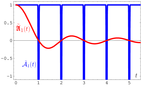
Figure 3: Illustration of the Laplace images of the one-loop analytic couplings in the Euclidean $(\tilde{{\cal A}}_{1}(t))$ and in the Minkowski space $(\tilde{\mathfrak{A}}_{1}(t))$.

Though we have initially assumed that $k>0$ and $\nu>0$, these Laplace conjugates generate, in turn, the following images that can be analytically extended to any real $\nu,~{}L$, and $L_{\sigma}$ (we display again the loop label ($l=1$) explicitly for the sake of comparison later on)

$$a^{\nu}_{(1)} = \frac{1}{L^{\nu}}\,,$$ (25)

$${\cal A}^{(1)}_{\nu}(L) = \frac{1}{L^{\nu}}-\frac{F(e^{-L},1-\nu)}{\Gamma(\nu)}\,,$$ (26)

$${\mathfrak{A}}^{(1)}_{\nu}(L_{s}) = \frac{\sin\left[(\nu-1)\arccos\left(L_{s}/\sqrt{(L_{s}^{2}+\pi^{2})}\right)\right]}{\pi\,(\nu-1)\left(L_{s}^{2}+\pi^{2}\right)^{(\nu-1)/2}}\,,$$ (27)

where the Dirac comb gives rise to the transcendental Lerch function, $F(z,\nu)$ BE53 , that serves as a Landau-pole remover for any $\nu$, and the oscillating curve amounts to elementary functions, confirming the result given in Eq. (19). The last expression is a new result of the present analysis and has been derived by taking recourse to the last entry of Eq. (24). It is worth emphasizing that ${\cal A}^{(1)}_{\nu}(L)$ and ${\mathfrak{A}}^{(1)}_{\nu}(L_{s})$ are entire functions of their corresponding arguments.

III.2 Properties of timelike vs. spacelike couplings for any real index $\nu$

1. From inspection of the relations (8), (9), and recalling that asymptotically as $L\to\infty$ both analytic couplings, ${\cal A}_{\nu}(L)$ and ${\mathfrak{A}}_{\nu}(L_{s})$, tend to the same standard coupling $a^{\nu}(L)$, one may ask about the mutual behavior of these couplings for finite values of their arguments. Despite the asymptotic symmetry of the couplings, for finite arguments this symmetry is distorted MS97 ; MiSol97 , albeit the couplings are equal at the origin, i.e., for $Q^{2}=s\to 0$, or equivalently, $L=L_{s}\to-\infty$. This “distorting-mirror” effect MS97 ; MiSol97 is an interesting property of the analytic couplings and was originally established for integer powers of the coupling. It is symbolically expressed through the operation

$${\cal A}^{(l)}_{\nu}(Q^{2})=\hat{D}\big{[}{\mathfrak{A}}^{(l)}_{\nu}(s)\big{]}$$ (28)

(see Eq. (8)), which we now generalize to be valid for any real index $\nu$. Its content may become evident from the following expressions for $L=L_{s}=0$:

$${\mathfrak{A}}_{\nu}(0)=\frac{\sin\left[(\nu-1)\pi/2\right]}{(\nu-1)\,\pi^{\nu}}: {\mathfrak{A}}_{1}(0)=\frac{1}{2},~{}{\mathfrak{A}}_{2}(0)=\frac{1}{\pi^{2}},~{}{\mathfrak{A}}_{3}(0)=0,~{}{\mathfrak{A}}_{4}(0)=-\frac{1}{3\pi^{4}},~{}~{}~{}~{}$$ (30)

$$\displaystyle{\mathfrak{A}}_{\frac{1}{2}}(0)=\frac{\sqrt{2}}{\pi^{1/2}},~{}~{}~{}{\mathfrak{A}}_{\frac{5}{2}}(0)=\frac{\sqrt{2}}{3\pi^{5/2}},~{}{\mathfrak{A}}_{\frac{7}{2}}(0)=-\frac{\sqrt{2}}{5\pi^{7/2}}$$

$${\cal A}_{\nu}(0)=-\frac{\zeta(1-\nu)}{\Gamma(\nu)}: {\cal A}_{1}(0)=\frac{1}{2},~{}{\cal A}_{2}(0)=\frac{1}{12},~{}{\cal A}_{3}(0)=0,~{}{\cal A}_{4}(0)=-\frac{1}{720}\,$$ (32)

$$\displaystyle{\cal A}_{\frac{1}{2}}(0)=\frac{-\zeta(\frac{1}{2})}{\pi^{1/2}},~{}{\cal A}_{\frac{5}{2}}(0)=\frac{\zeta(\frac{5}{2})}{4\pi^{5/2}},{\cal A}_{\frac{7}{2}}(0)=-\frac{\zeta(\frac{7}{2})}{8\pi^{7/2}},$$

where $\zeta(\nu)$ is the Riemann $\zeta$ function. These couplings are interrelated by the equation

$${\cal A}_{\nu}(0)=\left[\frac{(\nu-1)\,\zeta(\nu)}{2^{\,\nu-1}}\right]{\mathfrak{A}}_{\nu}(0)$$ (33)

with the coefficient in the bracket providing a quantitative measure for the magnitude of the distortion for any $\nu\in\mathbb{R}$. For a graphic illustration of the “distorted mirror symmetry” effect, we refer the interested reader to MS97 ; Shi01 ; Shi05 .

2. As we have shown in BMS05 for the Euclidean couplings, the parameters ${\cal A}_{-\nu}$ play the role of the “inverse powers” of ${\cal A}_{1}$ that may be considered as the images of $a_{s}^{-\nu}$. This property extends also to the Minkowski region, so that the set $\big{\{}{\cal A}_{-\nu},{\mathfrak{A}}_{-\nu}\big{\}}$ corresponds to analytic images of $a^{-\nu}$ in the Euclidean and the Minkowski space, respectively, for arbitrary $\nu$ values. This allows us to demonstrate the “distorted mirror” effect in analytic form as follows

$$\begin{array}[]{llll}{\mathfrak{A}}_{0}(L_{s})=1\,,&{\mathfrak{A}}_{-1}(L_{s})=L_{s}\,,&{\mathfrak{A}}_{-2}(L_{s})=L_{s}^{2}-\pi^{2}/3\,,&{\mathfrak{A}}_{-3}(L_{s})=L_{s}(L_{s}^{2}-\pi^{2})\,,\ldots\\ {\cal A}_{0}(L)=1\,,&{\cal A}_{-1}(L)=L\,,&{\cal A}_{-2}(L)=L^{2}\,,&{\cal A}_{-3}(L)=L^{3}\,,\ldots\end{array}$$ (36)

Note that the expressions for ${\mathfrak{A}}_{-n}$, given by Eq. (36), can be linked to ${\cal A}_{-n}$, in analogy to (28), by means of the transformation

$${\cal A}_{-n}(Q^{2})=\hat{D}\big{[}{\mathfrak{A}}_{-n}(s)\big{]}\,.$$ (37)

[See Eq. (19) in ChKS97 for an earlier implicit derivation of these expressions, employing transformation (8) in terms of the powers of $L_{s}$ (or in terms of ${\mathfrak{A}}_{-n}(s)$ in our notation)]. A useful all-order formula to analytically continue logarithms under the $\hat{D}$ transformation (see item 3 in Appendix B) has been presented in BKM01 .

   

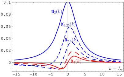
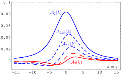
Figure 4: Comparison of the Minkowski (left panel) and the Euclidean (right panel) analytic couplings, ${\mathfrak{A}}_{\nu}(k=L_{s})$ and ${\cal A}_{\nu}(k=L)$, respectively, for incremental changes of the index $\nu$ in the range 2 to 3.

3. Moreover, the analytic couplings in both regions $(Q^{2},s)$, or equivalently, $(L,~{}L_{s})$, have the following symmetry (respectively, asymptotic) properties:

$$\begin{array}[]{lll}{\mathfrak{A}}_{m}(L_{s})=(-1)^{m}{\mathfrak{A}}_{m}(-L_{s})\,,&{\cal A}_{m}(L)=(-1)^{m}{\cal A}_{m}(-L)&~{}\text{for}~{}m\geq 2\,,\ m\in\mathbb{N}\,;\\ {\mathfrak{A}}_{m}(-\infty)={\cal A}_{m}(-\infty)=\delta_{m,1}\,,&{\mathfrak{A}}_{m}(\infty)={\cal A}_{m}(\infty)=0&~{}\text{for}~{}m\in\mathbb{N}\,.\end{array}$$ (40)

To reveal the details of behavior of the generalized analytic couplings ${\mathfrak{A}}_{\nu}(L_{s})$ and ${\cal A}_{\nu}(L)$ and make the above statements more transparent, we illustrate them in Fig. 4 in terms of two graphics, which display the rate of change of these functions with respect to the index $\nu$ and the argument $L$. Inspection of this figure in conjunction with Eq. (40) provides also information about how the zeros of the couplings occur.

III.3 Extension to higher loops and convergence of FAPT in the Minkowski vs. the Euclidean region

The last topic of this section is to extend our results to higher loops and to discuss the convergence properties of FAPT in the timelike region. In the following exposition, we shall employ, for the sake of simplicity, a special notation for the derivatives with respect to the index $\nu\in\mathbb{R}$ of the non-power expansion and define

$${\cal D}^{k}\,{{\cal A}_{\nu}\choose{\mathfrak{A}}_{\nu}}\equiv\frac{d^{k}}{d\nu^{k}}\,{{\cal A}_{\nu}\choose{\mathfrak{A}}_{\nu}}\,.$$ (41)

In our previous paper BMS05 we have obtained an expansion of the two-loop analytic coupling ${\cal A}_{\nu}^{(2)}(L)$ in terms of the one-loop analytic coupling ${\cal A}_{\nu}^{(1)}(L)$ (see Eq. (3.29) in BMS05 ). Due to the linearity of this expression in ${\cal A}_{\nu}^{(1)}(L)$, we can immediately rewrite it for timelike couplings—see Appendix C, Eqs. (114a), (114b)—by virtue of Eq. (113) to obtain the two-loop result

$${\mathfrak{A}}_{1}^{(2)}={\mathfrak{A}}_{1}^{(1)}+c_{1}\nu{\cal D}{\mathfrak{A}}_{\nu=2}^{(1)} + c_{1}^{2}\left[{\cal D}^{2}+{\cal D}-1\right]{\mathfrak{A}}_{\nu=3}^{(1)}$$ (42)

$$+ c_{1}^{3}\left[{\cal D}^{3}+\frac{5}{2}{\cal D}^{2}-2{\cal D}-\frac{1}{2}\right]{\mathfrak{A}}_{\nu=4}^{(1)}+{\cal O}\left({\cal D}^{4}{\mathfrak{A}}_{\nu=5}^{(1)}\right)\,,~{}~{}~{}$$

where we employed the auxiliary expansion parameter $c_{1}=b_{1}/b_{0}^{2}$.

Next, we test the quality of the two-loop expansion of the analytic-coupling images of $a_{(2)}$ and $\left(a_{(2)}\right)^{2}$ in the Minkowski region in comparison with the Euclidean one (refraining from displaying the latter because it is completely analogous—see Appendix C). In doing so, we define the following quantities for $\nu=1$ and $\nu=2$:

• NNLO, i.e., retaining terms up to order $c_{1}^{2}$

  $$\Delta_{3}\left({\mathfrak{A}}_{1}\right) = \frac{{\mathfrak{A}}_{1}^{(1)}+c_{1}\,{\cal D}\,{\mathfrak{A}}_{\nu=2}^{(1)}+c_{1}^{2}\,\left({\cal D}^{2}+{\cal D}-1\right)\,{\mathfrak{A}}_{\nu=3}^{(1)}}{{\mathfrak{A}}_{1}^{(2)}}\,-\,1\,;$$ (43)

• N³LO, i.e., retaining terms up to order $c_{1}^{3}$

  $$\Delta_{4}\left({\mathfrak{A}}_{1}\right) = \Delta_{3}\left({\mathfrak{A}}_{1}\right)+\frac{c_{1}^{3}\left({\cal D}^{3}+\frac{5}{2}\,{\cal D}^{2}\,-2\,{\cal D}\,-\frac{1}{2}\right){\mathfrak{A}}_{\nu=4}^{(1)}}{{\mathfrak{A}}_{1}^{(2)}}\,;$$ (44)

• N⁴LO, i.e., retaining terms up to order $c_{1}^{4}$ (cf. Eq. (47c))

  $${\mathfrak{A}}_{2}^{(2);\text{MFAPT}} = {\mathfrak{A}}_{2}^{(1)}+2\,c_{1}\,{\cal D}\,{\mathfrak{A}}_{\nu=3}^{(1)}+c_{1}^{2}\,\left(3\,{\cal D}^{2}+2\,{\cal D}-2\right)\,{\mathfrak{A}}_{\nu=4}^{(1)}$$

  $$~{}~{}~{}~{}~{}+c_{1}^{3}\,\left(4\,{\cal D}^{3}+7\,{\cal D}^{2}\,-6\,{\cal D}\,-1\right)\,{\mathfrak{A}}_{\nu=5}^{(1)}$$

  $$~{}~{}~{}~{}~{}+c_{1}^{4}\left(5{\cal D}^{4}+\frac{47}{3}{\cal D}^{3}-8{\cal D}^{2}-11{\cal D}+\frac{10}{3}\right){\mathfrak{A}}_{\nu=6}^{(1)}~{}~{}~{}$$ (45)

with analogous expressions for $\Delta_{3}\left({\cal A}_{\nu}\right)$ and $\Delta_{4}\left({\cal A}_{\nu}\right)$, obtained by using the evident substitution ${\mathfrak{A}}\rightarrow{\cal A}$.

   

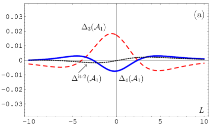
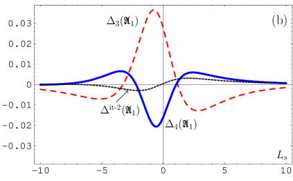
Figure 5: (a): The dashed red line corresponds to $\Delta_{3}({\cal A}_{1})$, whereas the solid blue line represents $\Delta_{4}({\cal A}_{1})$. (b): The dashed red line denotes $\Delta_{3}({\mathfrak{A}}_{1})$ and the solid blue line $\Delta_{4}({\mathfrak{A}}_{1})$. The dotted black line indicates $\Delta^{\text{it-2}}({\cal A}_{1})$ (left panel) and $\Delta^{\text{it-2}}({\mathfrak{A}}_{1})$ (right panel).

Figure 5 illustrates the convergence quality of the FAPT expansion in the spacelike and the timelike regions in terms of the quantities $\Delta_{n}$, defined above, that encapsulate the deviation of our approximations from the exact results. In addition, we consider the auxiliary quantity $\Delta^{\text{it}-2}$ (dotted black line) for the spacelike ($L$) and the timelike ($L_{s}$) regions, defined by the respective expressions

$$\Delta^{\text{it}-2}({\cal A}_{\nu})=\frac{{\cal A}_{\nu}^{(2)\text{it}-2}-{\cal A}_{\nu}^{(2)}}{{\cal A}_{\nu}^{(2)}}\,;\quad\Delta^{\text{it}-2}({\mathfrak{A}}_{\nu})=\frac{{\mathfrak{A}}_{\nu}^{(2)\text{it}-2}-{\mathfrak{A}}_{\nu}^{(2)}}{{\mathfrak{A}}_{\nu}^{(2)}}\,,$$ (46)

which, as one sees, result from replacing the exact spectral density (cf. (105)) by its second iteration (details are relegated to Appendix B).

From Fig. 5 one observes that the convergence of ${\cal A}_{1}^{(2)}$ and ${\mathfrak{A}}_{1}^{(2)}$ at the N³LO of the expansion in the auxiliary parameter $c_{1}$ is sufficiently accurate. In the Euclidean case (left panel), the errors—defined by $\Delta_{3}^{\text{FAPT}}\left({\cal A}_{1}\right)$, (dashed red line) and $\Delta_{4}^{\text{FAPT}}\left({\cal A}_{1}\right)$ (solid blue line)—induced by the non-power-series expansion are by a factor of two less than those in the Minkowski case (right panel): $\Delta_{3}^{\text{MFAPT}}\left({\mathfrak{A}}_{1}\right)$ (dashed red line) and $\Delta_{4}^{\text{MFAPT}}\left({\mathfrak{A}}_{1}\right)$ (solid blue line). The largest error results around $L=L_{s}=0$, but already for $|L|>2$ the uncertainty is less than a few per mil, rendering the convergence of the expansion highly reliable. Deriving the two-loop explicit expression

$${\mathfrak{A}}_{\nu}^{(2)} = {\mathfrak{A}}_{\nu}^{(1)}+c_{1}\,\nu\,{\cal D}\,{\mathfrak{A}}_{\nu+1}^{(1)}+c_{1}^{2}\,\nu\left[\frac{\nu+1}{2!}\,{\cal D}^{2}\,+\,{\cal D}\,-\,1\right]{\mathfrak{A}}_{\nu+2}^{(1)}~{}~{}~{}$$ (47a)

$$+ c_{1}^{3}\,\nu\left[\frac{(\nu+1)(\nu+2)}{3!}\,{\cal D}^{3}\,+\,\frac{2\,\nu+3}{2}\,{\cal D}^{2}+\,(1+\nu){\cal D}\,-\,\frac{1}{2}\right]{\mathfrak{A}}_{\nu+3}^{(1)}~{}~{}~{}$$ (47c)

$$+ c_{1}^{4}\,\nu\left[\frac{(\nu+1)(\nu+2)(\nu+3)}{4!}\,{\cal D}^{4}\,+\frac{3\,\nu^{2}+12\,\nu+11}{6}\,{\cal D}^{3}-\frac{\nu^{2}+2\,\nu}{2}\,{\cal D}^{2}\right.$$

$$\left.~{}~{}~{}~{}~{}~{}~{}-\frac{3\,\nu+5}{2}\,{\cal D}\,+\frac{3\,\nu+4}{6}\right]{\mathfrak{A}}_{\nu+4}^{(1)}+{\cal O}\left({\cal D}^{5}\,{\mathfrak{A}}_{\nu+5}^{(1)}\right)\,,$$

that is extended to the three-loop order of the running coupling in Appendix C (Eqs. (114a) to (114c)), a similar quality of convergence can be established for any desired fractional value of the index $\nu$.

   

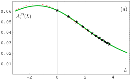
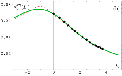
Figure 6: (a): The dashed red line corresponds to ${\cal A}_{2}^{(2);\text{FAPT}}(L)$, computed analytically via Eqs. (114a)–(114c) (for $c_{2}=0$), whereas the solid green line represents the exact expression for ${\cal A}_{2}^{(2)}(L)$, cf. Eqs. (5) and (105). (b): The dashed red line denotes ${\mathfrak{A}}_{2}^{(2);\text{MFAPT}}(L_{s})$, computed analytically via Eq. (45), whereas the solid green line represents the exact result for ${\mathfrak{A}}_{2}^{(2)}(L_{s})$, given by Eq. (108). On both panels, we also indicate by ★ the results of Magradze, presented in KM03 ; Mag03u .

In Figure 6 we show the results of the exact and the approximate calculation of ${\cal A}_{2}^{(2);\text{FAPT}}(L)$ and ${\mathfrak{A}}_{2}^{(2);\text{MFAPT}}(L_{s})$. This figure also includes the results (denoted by the symbol ★) obtained before by Magradze Mag03u . One observes that the agreement between his numerical estimates and our more elaborated calculations is excellent. We take the opportunity to remark that our opposite statements in BMS05 , notably Figure 4, were incorrect owing to an error in our code. This bug has now been eliminated, so that Magradze’s numerical results are fully supported by our calculation of the exact expressions for both analytic images ${\cal A}_{2}^{(2)}$ and ${\mathfrak{A}}_{2}^{(2)}$.

In concluding this section, it is worth listing the advantages of our calculation: (i) a good convergence of the non-power-series expansion, (ii) full control over the region in $L_{s}$ (correspondingly $L$), in which the maximum uncertainty occurs, making possible systematic improvements, and (iii) and most important for practical applications, a considerably reduced uncertainty level of the expansion in the physically interesting region, say, beyond $1$ GeV, (which corresponds to $L=2$) of only a few per mil.

IV Scalar correlator and Higgs boson decay into hadrons in MFAPT

To bring out the contrast with the original APT and effect the advantages and the utility of the (M)FAPT machinery with regard to the conventional perturbative expansion, we consider in this section the decay width of the Higgs boson into a bottom-antibottom pair, $\Gamma(\text{H}\to b\bar{b})$, using a multi-loop approximation. We stress in this context again that, though there are no ghost singularities in the Minkowski space owing to the strong coupling, the analytic continuation from the spacelike to the timelike region entails so-called ‘kinematical’ $\pi^{2}$ terms (see, for instance, BCK05 ) that can amount to pretty large contributions as the order of the perturbative expansion increases. Hence, even at high energies, relevant for the Higgs decay, the inclusion of these terms to all orders of the perturbative expansion is mandatory, albeit a difficult task. It is exactly this issue that singles out the utility of MFAPT because within such a perturbative approach, the analytic couplings contain all the aforementioned $\pi^{2}$ terms inherently by construction.

Our calculation of $\Gamma(\text{H}\to b\bar{b})$ via $R_{\text{S}}$ will be carried out in the $\overline{\text{MS}\vphantom{{}^{1}}}$ scheme and will include the evolution of both the coupling and the $b$-quark mass. Special attention will be given below to the origin of the $\alpha_{s}$ corrections in order to distinguish between the loop expansion and the loop evolution. In the following, we will compare our results with those obtained in the $\overline{\text{MS}\vphantom{{}^{1}}}$ scheme in Refs. Che96 ; ChKS97 ; BKM01 ; BCK05 , where the notation $\displaystyle a_{s}=\alpha_{s}/\pi$ (called “couplant”) was extensively used. For the sake of a better presentation of our results in comparison with the existing ones, just mentioned, it is useful to introduce the following abbreviation

$$\left[\left(a_{s}(s)\right)^{\nu}\right]_{\text{an}}={\mathfrak{a}}_{\nu}^{(l)}(s)\equiv\left(\frac{4}{b_{0}}\right)^{\nu}\,{\mathfrak{A}}_{\nu}^{(l)}(s)\,.$$ (48)

IV.1 Standard perturbation-theory analysis of $\mathbf{R}_{\text{S}}$

The Higgs-boson decay into a bottom-antibottom pair can be expressed in QCD by means of the correlator

$$\Pi(Q^{2})=(4\pi)^{2}i\int dxe^{iqx}\langle 0|\;T[\;J^{\text{S}}_{b}(x)J^{\text{S}}_{b}(0)\,]\;|0\rangle$$

of two quark scalar (S) currents in terms of the discontinuity of its imaginary part Djo05 , i.e., $R_{\text{S}}(s)=\textbf{Im}\,\Pi(-s-i\epsilon)/{(2\pi\,s)}$, so that the width reads

$$\Gamma(\text{H}\to b\bar{b})=\frac{G_{F}}{4\sqrt{2}\pi}M_{\text{H}}m_{b}^{2}(M_{\text{H}})R_{\text{S}}(s=M_{\text{H}}^{2})\,.$$ (49)

Above, $Q^{2}=-q^{2}$ and $J^{\text{S}}_{b}=\bar{\Psi}_{b}\Psi_{b}$ is the scalar current for bottom quarks with mass $m_{b}$, coupled to the scalar Higgs boson with mass $M_{\text{H}}$. Direct multi-loop calculations are usually performed in the Euclidean (spacelike) region for the corresponding Adler function $D_{\text{S}}$ Che96 ; BCK05 ; BKM01 , where QCD perturbation theory works. Hence, we write

$$\widetilde{D}_{\text{S}}(Q^{2};\mu^{2}) = 3\,m_{b}^{2}(Q^{2})\left[1+\sum_{n\geq 1}d_{n}(Q^{2}/\mu^{2})~{}a_{s}^{n}(\mu^{2})\right]\,,$$ (50)

using, as announced above, the notation $\displaystyle a_{s}={\alpha_{s}/\pi}$. Connecting to our discussion in Sec. II below Eq. (4), and adjusting to the scalar case, we now write the results of the ‘standard machinery’ (see, for instance, ChKS97 ):

$$\widetilde{R}_{\text{S}}(s)\equiv\widetilde{R}_{\text{S}}(s,s)=3m^{2}_{b}(s)\left[1+\sum_{n\geq 1}r_{n}~{}a_{s}^{n}(s)\right]\,.$$ (51)

The coefficients $r_{n}$ contain characteristic ‘$\pi^{2}$ terms’ due to the (integral) transformation $\hat{R}$ of the powers of the logarithms appearing in $\widetilde{D}_{\text{S}}$ (cf. Eq. (50)), as it was discussed in the beginning of Sec. II. Recall that in the case of $\widetilde{R}_{\text{S}}(s)$, these logarithms stem from two different sources: one is the running of $\alpha_{s}$ in $\widetilde{D}_{\text{S}}$, in analogy to Eq. (4), the other is related to the evolution of $m_{b}^{2}(Q^{2})$. Therefore, the coefficients $r_{n}$ in (51) appear to be related to a) the coefficients $d_{n}$ in (3), the latter being directly calculable in the Euclidean space, and b) to a combination of the mass anomalous dimension $\gamma_{i}$ and the $\beta$-function coefficients $b_{j}$, multiplied by ‘$\pi^{2}$ powers’ BKM01 ; Che96 ; ChKS97 . It turns out that the influence of these $\pi^{2}$ terms can be substantial, as the following quite recent result, derived in BCK05 , demonstrates:

$$\left[{3m_{b}^{2}}\right]^{-1}\widetilde{R}_{\text{S}} = 1+5.667\,a_{s}+a_{s}^{2}\left[51.57-\underline{15.63}-N_{f}\left({1.907}-\underline{0.548}\right)\right]$$ (52)

$$~{}\,+a_{s}^{3}\left[648.7-\underline{484.6}-N_{f}\left(63.74-\underline{37.97}\right)+N_{f}^{2}\left(0.929-\underline{0.67}\right)\right]$$

$$~{}\,+a_{s}^{4}\left[9470.8-\underline{9431.4}-N_{f}\left(1454.3-\underline{1233.4}\right)\right.$$

$$~{}~{}~{}~{}~{}~{}~{}~{}~{}~{}\left.+N_{f}^{2}\left(54.78-\underline{45.10}\right)-N_{f}^{3}\left(0.454-\underline{0.433}\right)\right]\,.$$

For emphasis, we have underlined the contributions of those $\pi^{2}$ terms which originate from the analytic continuation. As one can readily verify, the total amount of these terms is of the order of the original coefficients $d_{n}$, in particular, as regards the coefficient $d_{4}$. This makes it apparent that such terms have to be taken into account in all orders of the perturbative expansion. We stress that this is exactly the advantage provided by the analytic machinery, developed here and in BMS05 , and this conceptual advantage arises naturally without any additional optimization procedure. Indeed, in FAPT we do not need to expand the renormalization factors into a truncated series of logarithms; instead we can transform them ‘as a whole’ by means of the $\textbf{A}_{\text{M}}$-operation.

To complete the presentation of the standard analysis, let us display the final result at the ${\cal O}(a_{s}^{4})$, taken from Ref. BCK05 :

$$\left[{3m_{b}^{2}}\right]^{-1}\widetilde{R}_{\text{S}} = 1+5.6668\,a_{s}+29.147\,a_{s}^{2}+41.758\,a_{s}^{3}-825.7\,a_{s}^{4}$$ (53)

$$= 1+0.2075+0.0391+0.0020-0.00148\,.$$ (54)

Note that in Eq. (54) $a_{s}=a_{s}(M_{\text{H}}^{2})=0.0366$ is chosen, which corresponds to the Higgs boson mass $M_{\text{H}}=120$ GeV.

IV.2 FAPT analysis of $\widetilde{R}_{\text{S}}$

We turn now our attention to effects related to the renormalization of the bottom-quark mass. For the running mass $m_{(l)}(Q^{2})$, in the $l$-loop approximation, one has the following general solution of the RG equation

$$m_{(l)}^{2}(Q^{2}) = m_{(l)}^{2}(\mu^{2})\,\exp\left[2\int_{a_{s}(\mu^{2})/4}^{a_{s}(Q^{2})/4}\frac{\gamma_{m}(x)}{\beta(x)}\,dx\right]$$ (55)

$$= m_{(l)}^{2}(\mu^{2})\,\frac{\left[a_{s}(Q^{2})\right]^{\nu_{0}}f_{(l)}(a_{s}(Q^{2}))}{\left[a_{s}(\mu^{2})\right]^{\nu_{0}}f_{(l)}(a_{s}(\mu^{2}))}\,,$$ (56)

where

$$\nu_{0}=2\frac{\,\gamma_{0}}{b_{0}}$$ (57)

and the function $f_{(l)}(a_{s})$, given by

$$f_{(l)}(a_{s})=\exp\left[2\int_{0}^{a_{s}/4}\left(\frac{\gamma_{m}^{(l)}(x)}{\beta^{(l)}(x)}-\frac{\gamma_{0}\,x}{b_{0}\,x^{2}}\right)\,dx\right]\,,$$ (58)

accumulates the effects of the second- and higher-loop evolution of $m_{(l)}^{2}(Q^{2})$ with $Q^{2}$. In the one-loop approximation ($l=1$), $f_{(l)}(a_{s})$ is set by definition equal to unity. On the other hand, for $l=2$ and $l=3$ we obtain

$$f_{(2)}(a_{s})=\left[1+\delta_{1}\,a_{s}\right]^{\nu_{1}}\quad\text{with~{}~{}~{}}\delta_{1}=\frac{b_{1}}{4b_{0}}=\frac{c_{1}b_{0}}{4}\,,~{}\nu_{1}=2\left(\frac{\gamma_{1}}{b_{1}}-\frac{\gamma_{0}}{b_{0}}\right)$$ (59)

and

$$f_{(3)}(a_{s})=\left[1+\delta_{1}\,a_{s}+\delta_{2}\,a_{s}^{2}\right]^{\nu_{20}}\exp\left[\nu_{21}\,\arccos\left(\frac{1+\delta_{1}\,a_{s}/2}{\sqrt{1+\delta_{1}\,a_{s}+\delta_{2}\,a_{s}^{2}}}\right)\right]$$ (60a)

with

$$\delta_{2}=\frac{b_{2}}{16b_{0}}\,,~{}\nu_{20}=\left(\frac{\gamma_{2}}{b_{2}}-\frac{\gamma_{0}}{b_{0}}\right)\,,~{}\nu_{21}=\frac{-2\,b_{1}}{\sqrt{4b_{2}b_{0}-b_{1}^{2}}}\left(\frac{\gamma_{2}}{b_{2}}-2\frac{\gamma_{1}}{b_{1}}+\frac{\gamma_{0}}{b_{0}}\right)\,.$$ (60b)

Introducing the RG-invariant quantity $\hat{m}_{(l)}$, see, e.g., BKM01 ; KKP00 ,

$$\hat{m}_{(l)} = m_{(l)}(\mu^{2})\left\{\left[a_{s}(\mu^{2})\right]^{\nu_{0}}f_{(l)}(a_{s}(\mu^{2}))\right\}^{-1/2}\,,$$ (61)

one can rewrite Eq. (56) in the form

$$m_{(l)}^{2}(Q^{2}) = \hat{m}_{(l)}^{2}\left[a_{s}(Q^{2})\right]^{\nu_{0}}f_{(l)}(a_{s}(Q^{2}))\,,$$ (62)

where the expansion of $f_{(l)}(x)$ at the three-loop order is given by

$$f_{(l)}(a_{s}) = 1+a_{s}\,\frac{b_{1}}{2b_{0}}\left(\frac{\gamma_{1}}{b_{1}}-\frac{\gamma_{0}}{b_{0}}\right)+a_{s}^{2}\,\frac{b_{1}^{2}}{16\,b_{0}^{2}}\left[\frac{\gamma_{0}}{b_{0}}-\frac{\gamma_{1}}{b_{1}}+2\,\left(\frac{\gamma_{0}}{b_{0}}-\frac{\gamma_{1}}{b_{1}}\right)^{2}+\frac{b_{0}b_{2}}{b_{1}^{2}}\left(\frac{\gamma_{2}}{b_{2}}-\frac{\gamma_{0}}{b_{0}}\right)\right]$$ (63)

$$+ O\left(a_{s}^{3}\right)\,,$$

which is in one-to-one correspondence with Eq. (15) found by Chetyrkin in Che97 . [Note, however, that Chetyrkin expands instead the expression $\sqrt{f_{(l)}(x)}\equiv c(x)$ and uses different normalizations; viz., $\bar{\beta}_{n}=b_{n}/(4^{n}b_{0})$ and $\bar{\gamma}_{n}=\gamma_{n}/(4^{n}b_{0})$.] Keeping in mind the main purpose of our task, namely, the sequential “analytization” of $D$, we rewrite the RG Eq. (62) in the form of a power series to get

$$m_{(l)}^{2}(Q^{2}) = \hat{m}_{(l)}^{2}\,\left(a_{s}(Q^{2})\right)^{\nu_{0}}\left[1+\sum_{m\geq 1}^{\infty}e^{(l)}_{m}\,\left(a_{s}(Q^{2})\right)^{m}\right]\,,$$ (64)

where the coefficients $e^{(l)}_{m}$ depend implicitly on the RG parameters via Eq. (58). For the simplest case of a two-loop running, they can be written down explicitly:

$$e^{(2)}_{m} = \frac{\Gamma(\nu_{1}+1)\,}{\Gamma(m+1)\Gamma(\nu_{1}-m+1)}(\delta_{1})^{m}\,.$$ (65)

Substituting Eq. (64) for $m_{(l)}^{2}(Q^{2})$ into $\widetilde{D}_{\text{S}}(Q^{2})\equiv\widetilde{D}_{\text{S}}(Q^{2};Q^{2})$ in Eq. (50), one finds

$$\left[3\,\hat{m}_{b}^{2}\right]_{(l)}^{-1}\,\widetilde{D}^{(l)}_{\text{S}}(Q^{2})=\left(a^{(l)}_{s}(Q^{2})\right)^{\nu_{0}}+\sum_{n\geq 1}^{l}d_{n}\,\left(a^{(l)}_{s}(Q^{2})\right)^{n+\nu_{0}}+\sum_{m\geq 1}^{\infty}\Delta^{(l)}_{m}\,\left(a^{(l)}_{s}(Q^{2})\right)^{m+\nu_{0}}$$ (66)

with

$$\Delta^{(l)}_{m} = e_{m}^{(l)}+\sum_{k\geq 1}^{\textbf{min}[l,m-1]}d_{k}\,e_{m-k}^{(l)}\,.$$ (67)

The effects of mass evolution of the higher orders are collected in the third term on the RHS of Eq. (66) and have been purportedly separated from the original series expansion of $D$ (truncated at $n=l$), the latter being represented by the second term on the RHS of Eq. (66). In practice, for $Q\geq 2$ GeV, i.e., for $\alpha_{s}\leq 0.4$, the truncation at $m=l+4$ of the summation (64) produces a truncation error smaller than $0.01\%$.

To obtain $\widetilde{R}_{\text{S}}^{\text{MFAPT}}$, we recall the action of the $\textbf{A}_{\text{M}}$ operation in FAPT, as described in Sec. II, and consider the map of the quantity $\widetilde{D}_{\text{S}}^{(l)}(Q^{2})$ in Eq. (66) onto the Minkowski region. Following the “analytization” procedure illustrated in Fig. 2, we then obtain

$$\widetilde{R}_{\text{S}}^{(l)\text{MFAPT}}=\textbf{A}_{\text{M}}[D^{(l)}_{\text{S}}]=3\,\hat{m}_{(l)}^{2}\,\left[{\mathfrak{a}}_{\nu_{0}}^{(l)}+\sum_{n\geq 1}^{l}d_{n}{\mathfrak{a}}_{n+\nu_{0}}^{(l)}+\sum_{m\geq 1}\Delta_{m}^{(l)}{\mathfrak{a}}_{m+\nu_{0}}^{(l)}\right]\,,$$ (68)

where the superscript $l$ denotes the loop order of the evolution and fixes at the same time the order of the perturbative expansion of the $D_{S}$-function. The above expression contains, by means of the coefficients $\Delta_{n}^{(l)}~{}(~{}e^{(l)}_{k})$ and the couplings ${\mathfrak{a}}_{n+\nu_{0}}^{(l)}$, all RG terms contributing to this order, while the resummed $\pi^{2}$ terms are integral parts of the analytic couplings by construction.

IV.3 Comparison of different perturbative approaches to obtain $\widetilde{R}_{\text{S}}$

We list below the results obtained for the quantity $\widetilde{R}_{\text{S}}$ using different methods.

• Broadhurst, Kataev, and Maxwell (BKM) BKM01 utilized within the so-called “naive non-Abelianization” (NNA) approach an optimized power-series expansion, based on the “contour integration” technique, to compute $\widetilde{R}_{\text{S}}$. Their estimate, with one-loop running of $a_{s}$ and setting $a_{s}^{(l=1)}\equiv a_{s}$, reads (see Section 3.3 in BKM01 )

  $$\widetilde{R}_{\text{S}}^{(l=1)\text{BKM}} = 3\,\hat{m}^{2}_{(l=1)}\left(a_{s}\right)^{\nu_{0}}\left[A_{0}^{\text{BKM}}(a_{s})+\sum_{n\geq 1}d_{n}\,A_{n}^{\text{BKM}}(a_{s})\right],$$ (69)

  $${A}^{\text{BKM}}_{n}(a_{s}) = \frac{4}{b_{0}\,\pi\,\delta_{n}}{\left[1+\left(\frac{b_{0}\,\pi\,a_{s}}{4}\right)^{2}\right]}^{-\delta_{n}/2}\left(a_{s}\right)^{n-1}{\sin}\left({\delta}_{n}\arctan\left(\frac{b_{0}\,\pi\,a_{s}}{4}\right)\right),~{}~{}~{}~{}~{}~{}~{}$$ (70)

  $${\delta}_{n} = n+\nu_{0}-1\,.$$ (71)

  These new couplings ${A}^{\text{BKM}}_{n}(a_{s})$ and the whole result are closely related to our analytic approach at the one-loop level, as we will show shortly.

• Baikov, Chetyrkin, and Kühn (BChK) BCK05 have derived within the standard perturbative QCD at the ${\cal O}(a_{s}^{4})$, c.f. Eq. (52)), the following expression:

  $$\widetilde{R}_{\text{S}}^{(l=4)\text{BChK}} = 3\bar{m}^{2}(s)^{(l=4)}\left[1+\sum_{n\geq 1}^{4}r_{n}\left(a_{s}^{(l=4)}\right)^{n}\right]\,.$$ (72)

• Consider now the MFAPT equation (68) and recast it in the form

  $$\widetilde{R}_{\text{S}}^{(l)\text{MFAPT}}\! = \!3\,\hat{m}_{(l)}^{2}\left[{\mathfrak{a}}_{\nu_{0}}^{(l)}+\sum_{n\geq 1}^{l}d_{n}\,{\mathfrak{a}}_{n+\nu_{0}}^{(l)}+\sum_{m\geq 1}^{l+4}\Delta_{m}^{(l)}\,{\mathfrak{a}}_{m+\nu_{0}}^{(l)}\right]$$ (73)

  $$= \!3\,\hat{m}_{(l)}^{2}\left[{\mathfrak{a}}_{\nu_{0}}^{(l)}+\sum_{n\geq 1}^{l}d_{n}\left({\mathfrak{a}}_{n+\nu_{0}}^{(l)}+\sum_{m\geq 1}^{4}e_{m}^{(l)}\,{\mathfrak{a}}_{n+m+\nu_{0}}^{(l)}\right)+\sum_{m\geq 1}^{4}e_{m}^{(l)}{\mathfrak{a}}_{m+\nu_{0}}^{(l)}\right]\!,~{}~{}~{}~{}~{}~{}~{}~{}$$ (74)

  where we have truncated the “evolution series” at $m=l+4$, adopting the empirical recipe discussed after Eq. (67). Pay attention that the terms ${\mathfrak{a}}_{m+\nu_{0}}^{(l)}$ contain—by means of the index $\nu_{0}$—all $\gamma_{0}$ and $b_{0}$ terms, and also all $\pi^{2}$ terms, while the contributions of the higher-loop RG-dependent parts are accumulated in the coefficients $\Delta_{m}^{(l)}$—see Eqs. (62), (63) and also (66), (67)—in terms of the RG-parameters $\gamma_{i}$ and $b_{j}$.

Equation (73) can be considered as a generalization of the BKM “contour-improved” expansion in Eqs. (69)–(71). To see this, one should reduce the above expression to the one-loop case, by setting $\Delta_{m}^{(l)}\to 0$ and ${\mathfrak{a}}_{\nu}^{(l)}\to{\mathfrak{a}}_{\nu}^{(1)}$, with the aim to reproduce the “contour-improved” effective coupling in Eq. (69). In fact, taking into account the explicit expression (19) for ${\mathfrak{a}}_{\nu}^{(1)}$, one can readily find the relation

$${\mathfrak{a}}_{n+\nu_{0}}^{(1)}=\left(\frac{4}{b_{0}}\right)^{n+\nu_{0}}\,{\mathfrak{A}}_{n+\nu_{0}}^{(1)}=\left(a_{s}\right)^{\nu_{0}}A_{n}(a_{s})$$ (75)

recalling (70) and (71). This relation establishes the equivalence between the “contour-improved” effective coupling and the timelike analytic coupling ${\mathfrak{a}}_{\nu}^{(1)}$ in the one-loop approximation of MFAPT. The only difference between $\widetilde{R}_{\text{S}}^{(l=1)\text{BKM}}$ and $\widetilde{R}_{\text{S}}^{(l=1)\text{MFAPT}}$ stems from the summation in Eq. (69), which extends to all known $d_{n}$-coefficients, i.e., also to those up to $n=4$.

In Fig. 7, we display the final results for the quantity $\widetilde{R}_{\text{S}}^{(l)\text{MFAPT}}$ in Eq.(73) vs. the Higgs mass $M_{\text{H}}$ evaluating it for the cases of two ($l=2)$ and three ($l=3$) loops, with the goal to illustrate the effects of the “analytization” procedure in comparison with the standard approach. The solid blue line in both panels of this figure shows the prediction obtained with MFAPT and a fixed number of active flavors $N_{f}=5$. One appreciates that this curve lies only slightly (about $2\%$ for $l=3$) above the standard result $\widetilde{R}_{\text{S}}^{(l=4)\text{BChK}}$, illustrated by the dashed red line. This is mainly due to the somewhat larger values of the perturbative coefficients $d_{n}$ within MFAPT relative to the standard ones, $r_{n}$. At the same time, the dotted green line, which corresponds to $\widetilde{R}_{\text{S}}^{(l=1)\text{BKM}}$, Eq. (4.22), turns out to lie lower than the BChK prediction by about 7 to 8%. Note that if one sets $\Lambda_{N_{f}=5}=221$ MeV, as dictated by the one-loop perturbative QCD analysis of the DIS data KPS02 , then the BKM curve, corresponding to this value, will end up to lie higher than the BHhK prediction by 8%.

  

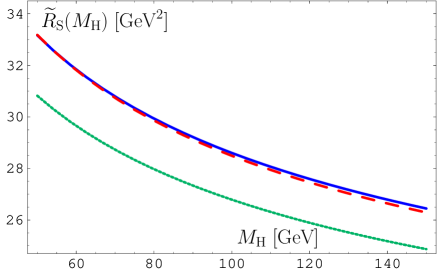
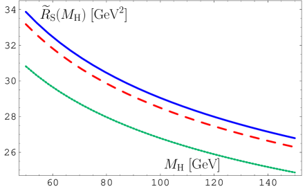
Figure 7: Illustration of the calculation of the perturbative series of the quantity $\widetilde{R}_{\text{S}}(M^{2}_{\text{H}})$ in different approaches within the $\overline{\text{MS}\vphantom{{}^{1}}}$ scheme: standard perturbative QCD ChKS97 ; BCK05 at the loop level $l=4$ (dashed red line, $\Lambda_{N_{f}=5}=231$ MeV); BKM estimates, by taking into account the $O(\left(a_{s}\right)^{\nu_{0}}A_{4}(a_{s}))$-terms, BKM01 (dotted green line, $\Lambda_{N_{f}=5}=111$ MeV); and finally MFAPT from (74) for $N_{f}=5$ (solid blue line), displayed for $l=2$ (left panel, $\Lambda_{N_{f}=5}=263$ MeV) and $l=3$ (right panel, $\Lambda_{N_{f}=5}=261$ MeV). All $\Lambda_{N_{f}=5}$ scales are defined in such a way as to reproduce the corresponding couplings with the value 0.120 at $s=m_{Z}^{2}$.

Table 1: Comparison of the perturbative-series convergence in terms of the associated perturbative orders, using for the Higgs boson mass the value $M_{\text{H}}=120$ GeV and employing different expansions within the $\overline{\text{MS}\vphantom{{}^{1}}}$ scheme: (i) Standard perturbative QCD ChKS97 ; BCK05 , (ii) BKM BKM01 , and (iii) MFAPT at the two- and the three-loop level of evolution with the number of flavors fixed to $N_{f}=5$ and $s=\left[120~{}\text{GeV}\right]^{2}$.

Expansion approach used	$\widetilde{R}_{\text{S}}(s)$	$O(1)$	$O(a_{s})$	$O(a_{s}^{2})$	$O(a_{s}^{3})$	$O(a_{s}^{4})$
standard QCD BCK05	27.44 GeV2	80.2%	16.6%	3.1%	0.2%	$-0.1$%
MFAPT	$\widetilde{R}_{\text{S}}(s)$	$O({\mathfrak{a}}_{\nu_{0}}^{(l)})$	$O({\mathfrak{a}}_{1+\nu_{0}}^{(l)})$	$O({\mathfrak{a}}_{2+\nu_{0}}^{(l)})$	$O({\mathfrak{a}}_{3+\nu_{0}}^{(l)})$	$O({\mathfrak{a}}_{4+\nu_{0}}^{(l)})$
BKM BKM01 (MFAPT for $l=1$)	31.89 GeV2	74.5%	17.7%	5.3%	1.8%	0.7%
MFAPT for $l=2$, this work	27.59 GeV2	79.5%	16.2%	4.3%
MFAPT for $l=3$, this work	28.07 GeV2	78.5%	16.1%	4.2%	1.2%

In Table 1 we show for the quantity $\widetilde{R}_{\text{S}}(s)$ a comparison of the perturbative series evaluated in different expansion approaches, discussed in the literature and in this work. One may conclude that the standard perturbation-theory series and MFAPT show a similar behavior, starting with the two-loop running. Because the coefficients $d_{n}$ of MFAPT are larger than the standard ones, $r_{n}$, due to the subtraction of the $\pi^{2}$ terms in the latter, the fixed-order MFAPT result for the quantity $\widetilde{R}_{\text{S}}(s)$ appears to be slightly larger than that of the standard perturbative QCD approach. However, the coupling parameters of MFAPT, ${\mathfrak{a}}_{\nu}$, contain the resummed contribution of an infinite series of $\pi^{2}$-terms that renders them ultimately smaller (for the same value of $\Lambda_{\text{QCD}}$) than the corresponding powers of the standard coupling, as it can be seen from Table 2.

Table 2: Comparison of the combined evolution effects on the ratio of MFAPT to the standard perturbation theory for the three-loop evolution case and fixing the number of flavors to $N_{f}=5$. For the sake of completeness, we also show the ratios of the associated perturbative coefficients $d_{n}$ and $r_{n}$ and the approximate relative weights $\displaystyle\omega_{n}=r_{n}E_{n+\nu_{0}}^{(3)}/\sum_{i=0,...,3}r_{i}E_{i+\nu_{0}}^{(3)}$ of the corresponding contributions.

	$n=0$	$n=1$	$n=2$	$n=3$
$\displaystyle\big{[}{\cal E}_{n+\nu_{0}}^{(3)}\vphantom{{}^{\big{|}}}/{E_{n+\nu_{0}}^{(3)}}\big{]}_{s=(120~{}\text{GeV})^{2}}$	1.00	0.98	0.95	0.91
$d_{n}/r_{n}\vphantom{{}_{|}}$	1.00	1.00	1.44	8.46
relative weight $\omega_{n}\vphantom{{}_{|}}$	0.801	0.166	0.031	0.002

In order to demonstrate the combined effect of evolving the coefficients and the heavy quark mass at different orders of the perturbative expansion, we define the following factors for, respectively, the standard perturbation theory (PT) and for MFAPT:

$$E_{\nu}^{(l)}(s) = \left(a_{s}(s)\right)^{\nu}+\sum_{m\geq 1}^{4}e_{n}^{(l)}\left(a_{s}(s)\right)^{m+\nu}\,;$$ (76)

$${\cal E}^{(l)}_{\nu}(s) = {\mathfrak{a}}_{\nu}(s)+\sum_{m\geq 1}^{4}e_{n}^{(l)}{\mathfrak{a}}_{m+\nu}(s)\,.$$ (77)

Then Eqs. (72) and (74) can be rewritten as

$$\widetilde{R}_{\text{S}}^{(l)\text{PT}}=3\,\hat{m}_{(l)}^{2}\,\left[E_{\nu_{0}}^{(l)}(s)+\sum_{n\geq 1}^{l}r_{n}E_{n+\nu_{0}}^{(l)}(s)\right]\!;$$ (78)

$$\widetilde{R}_{\text{S}}^{(l)\text{MFAPT}}=3\,\hat{m}_{(l)}^{2}\,\left[{\cal E}_{\nu_{0}}^{(l)}(s)+\sum_{n\geq 1}^{l}d_{n}{\cal E}_{n+\nu_{0}}^{(l)}(s)\right]\,.$$ (79)

In order to understand the effect of “analytization”, we compare the values of ${\cal E}_{n+\nu_{0}}^{(l)}(s)$ with those of $E_{n+\nu_{0}}^{(l)}(s)$, and display their ratio in Table 2. Using the entries of this Table, one can easily estimate the relative enhancement of $\widetilde{R}_{\text{S}}^{(3)\text{MFAPT}}$ with respect to $\widetilde{R}_{\text{S}}^{(3)\text{PT}}$:

$$\frac{\widetilde{R}_{\text{S}}^{(3)\text{MFAPT}}}{\widetilde{R}_{\text{S}}^{(3)\text{PT}}}=\sum_{n\geq 0}^{3}\omega_{n}\,\frac{d_{n}}{r_{n}}\,\frac{{\cal E}_{n+\nu_{0}}^{(3)}(s)}{E_{n+\nu_{0}}^{(3)}(s)}=0.801+0.163+0.042+0.015=1.021\,,$$ (80)

$$\mbox{where}~{}\displaystyle\omega_{n}=r_{n}E_{n+\nu_{0}}^{(3)}/\sum_{i=0,\ldots,3}r_{i}E_{i+\nu_{0}}^{(3)}.$$ (81)

From this equation in conjunction with the values of $\omega_{n}$ (presented in Table 2), we see that the largest enhancement is provided for $n=3$ due to $d_{n}/r_{n}=8.46$, amounting to a $1.5\%$ contribution to $\widetilde{R}_{\text{S}}^{(3)\text{MFAPT}}$ out of $2.1\%$ in total. Evolution, which potentially could reduce this enhancement, because of the inclusion into the analytic coupling of the resummed $\pi^{2}$ terms, notably, ${\cal E}_{n+\nu_{0}}^{(3)}/{E_{n+\nu_{0}}^{(3)}}=0.91$, is too small to counterbalance it.

V Summary and Conclusions

This report has focused on the implementation of analyticity of QCD amplitudes both in the Euclidean and in the Minkowski space, the theoretical basis being provided by dispersion relations (to ensure causality) in conjunction with the renormalization group. The goal of the work was to elevate Analytic Perturbation Theory—initiated by Shirkov and Solovtsov SS97 —to a calculational paradigm for perturbative QCD applications, capable of providing singularity-free expressions for any real power of the strong coupling. Following the rationale that all quantities that may contribute to the spectral density should be included into the “analytization” procedure KS01 ; Ste02 , we have expanded the previously developed Fractional Analytic Perturbation Theory BMS05 from the spacelike to the timelike region.

The core issues of the investigation can be summarized as follows, starting with the benchmarks of the analytic couplings ${\cal A}_{\nu}^{(l)}(L)$ (spacelike) and ${\mathfrak{A}}_{\nu}^{(l)}(L_{s})$ (timelike) of (M)FAPT for an arbitrary real index $\nu$:

• $\left\{{\cal A}_{\nu}^{(l)}(L),{\mathfrak{A}}_{\nu}^{(l)}(L_{s})\right\}$ is analytic in $L$ (respectively, $L_{s}$) and also in the index $\nu\in\mathbb{Z}$; for $l=1$, see Eqs. (26) and (27); for $l=2$, see Sec. III C and also Mag05 (for integer indices). This implies the existence of any index derivative $\displaystyle\frac{d^{m}}{d\nu^{m}}\,\left\{{\cal A}_{\nu}^{(l)}(L),{\mathfrak{A}}_{\nu}^{(l)}(L_{s})\right\}$.

• ${\cal A}_{m}^{(l)}(-\infty)={\mathfrak{A}}_{m}^{(l)}(-\infty)=\delta_{1,m}$ for $m\in\mathbb{N}$ Shi98 and ${\cal A}_{\nu}^{(l)}(-\infty)={\mathfrak{A}}_{\nu}^{(l)}(-\infty)=0$ for $\nu>1$. This implies the existence of a universal IR fixed point.

• ${\mathfrak{A}}_{\nu}^{(l)}(L_{s}\to\infty)\to{\cal A}_{\nu}^{(l)}(L\to\infty)\to a^{\nu}_{(l)}(L\to\infty)$ have the correct UV asymptotics, dictated by the asymptotic freedom of QCD.

• The effect of the “distorted-mirror symmetry” with respect to $L$ and $L_{s}$, is exhibited analytically in terms of ${\cal A}^{(l)}_{\nu}(L)$ and ${\mathfrak{A}}^{(l)}_{\nu}(L_{s})$ for any real $\nu$.

• The “analytization” of expressions, like ${\cal L}_{\nu,m}^{(l)}(L)=\textbf{A}_{\text{E}}\left[\left(a_{(l)}(L)\right)^{\nu}L^{m}\right]$, ${\cal L}_{\nu,m}^{(l)}(L_{s})=\textbf{A}_{\text{M}}\left[\left(a_{(l)}(L)\right)^{\nu}L^{m}\right]$, which amount to ‘evolution logarithmic factors’ in $l$-order QCD perturbation theory, typical examples being logarithms of the factorization scale (appearing beyond the leading-order expansion), and significantly affecting the precision of perturbative calculations, becomes possible. Moreover, the insensitivity to the choice of the factorization scale BKS05 and a diminished dependence on the adopted renormalization scheme and scale setting has been achieved BPSS04 .

The following topics have been given particular attention:

1. We have presented a brief historical review of the “analytization” technology from early attempts in QED up to the most recent developments in QCD perturbation theory and phenomenology (Introduction), highlighting the strategy for resolving the conflict with analyticity in $Q^{2}$ of QCD “observables” in the perturbative regime.

2. In sections II and III we have worked out in detail the theoretical framework to deal with analytic versions of the strong coupling and its powers for any fractional (real) power, encompassing the spacelike and also the timelike region.

3. We have given closed-form expressions for the analytic-coupling images at the one-loop level both in the Euclidean, as well as in the Minkowski space. We have also provided explicit but approximate expressions at the two-loop level, which show excellent agreement with the exact but numerical results in terms of the Lambert function, found before by Magradze Mag03u —see Fig. 6. Three-loop (approximate) results have also been included and the fast convergence of the non-power-series expansion has been proved.

4. The major characteristics (advantages) of this machinery, studied in Sec. III, are: (i) a reduced uncertainty level of only a few per mil in a wide range of momentum (or energy) values, starting just above $1$ GeV, (ii) the high quality of the non-power-series expansion, evidenced by providing trustworthy analytic expressions for the strong coupling and its powers at the one, two- and three-loop level that are singularity free in the spacelike region and resum the $\pi^{2}$ terms (induced by analytic continuation) to all orders in the timelike domain.

5. The relevance of the developed framework for practical purposes in the Minkowski space has been effected in Sec. IV by applying it to the decay of a scalar Higgs boson to a $b\bar{b}$ pair, this task serving as a Proof-of-the-Concept-calculation. Specifically, we estimated the quantity $R_{\text{S}}$ at the four-loop level of the perturbative expansion (i.e., up to the coefficient $d_{3}$), having recourse to the coefficients and anomalous dimensions calculated by Chetyrkin and collaborators in Che96 ; ChKS97 . The main advantage of MFAPT here is that the coupling parameters ${\mathfrak{A}}_{\nu}$ inherently include the resummed contribution of an infinite series of those $\pi^{2}$-terms originating from the analytic continuation from the Euclidean to the Minkowski space. Technically, we could have also included the next correction, associated with the coefficient $d_{4}$, but this would be not worth the effort, given that the expected contribution would be about $0.5\%$.

In conclusion, we think that the analytic approach to QCD perturbation theory in the form advocated here has indeed been rather successful both in the spacelike and in the timelike region for the particular processes we have discussed in this work and elsewhere BMS05 ; BKS05 ; BPSS04 . The developed full-fledged machinery may improve our understanding of key issues of QCD reactions from the poorly understood low-momentum (spacelike) domain, where the Landau singularities are a serious obstacle in standard perturbative QCD (based on power-series expansions) up to the high-energy (timelike) region of several GeV. In conjunction with high-loop calculations in the latter case, the $\pi^{2}$ terms, entailed by analytic continuation, can significantly change the result in higher orders. A greater challenge, however, is to include into the approach gluon resummation and power corrections analytically, beyond the attempts in KS01 and BMS05 , with the aim to unravel the analytic structure of the involved amplitudes in the whole momentum (energy) range. Work in this direction is currently in progress.

Appendix A Two-loop renormalization-group solutions for the coupling

1. The expansion of the $\beta$-function is given by the RHS of the equation

$$\frac{d}{dL}\left(\frac{\alpha_{s}}{4\pi}\right)=\beta\left(\frac{\alpha_{s}}{4\pi}\right)=-b_{0}\left(\frac{\alpha_{s}}{4\pi}\right)^{2}-b_{1}\left(\frac{\alpha_{s}}{4\pi}\right)^{3}-b_{2}\left(\frac{\alpha_{s}}{4\pi}\right)^{4}\,-\ldots\,,$$ (82)

where $L=\ln(\mu^{2}/\Lambda^{2})$ and

$$b_{0} = \frac{11}{3}\,C_{\text{A}}-\frac{4}{3}\,T_{\text{R}}N_{f}\,;\qquad b_{1}=\frac{34}{3}\,C_{\text{A}}^{2}-\left(4C_{\text{F}}+\frac{20}{3}\,C_{\text{A}}\right)T_{\text{R}}N_{f};$$

$$b_{2} = \frac{2857}{54}C_{\text{A}}^{3}+2C_{\text{F}}^{2}T_{\text{R}}N_{f}-\frac{205}{9}C_{\text{F}}C_{\text{A}}T_{\text{R}}N_{f}-\frac{1415}{27}C_{\text{A}}^{2}T_{\text{R}}N_{f}+\frac{44}{9}C_{\text{F}}(T_{\text{R}}N_{f})^{2}$$ (83)

$$+\frac{158}{27}C_{\text{A}}(T_{\text{R}}N_{f})^{2}\,,$$

with $C_{\text{F}}=\left(N_{\text{c}}^{2}-1\right)/2N_{\text{c}}=4/3$, $C_{\text{A}}=N_{\text{c}}=3$, $T_{\text{R}}=1/2$, and $N_{f}$ denoting the number of active flavors. The corresponding three-loop RG equation for the coupling $a=b_{0}\,\alpha/(4\pi)$ is

$$\frac{da_{(3)}}{dL}=-a_{(3)}^{2}\left[1+c_{1}\,a_{(3)}+c_{2}\,a_{(3)}^{2}\right]\text{~{}~{}with~{}}c_{1}\equiv\frac{b_{1}}{b_{0}^{2}},~{}c_{2}\equiv\frac{b_{2}}{b_{0}^{3}}\,.$$ (84)

The solution of this RG equation at the two-loop level ($c_{2}=0$) assumes the form

$$\frac{1}{a_{(2)}}+c_{1}\ln\left[\frac{a_{(2)}}{1+c_{1}a_{(2)}}\right]=L\,.$$ (85)

The exact solution of Eq. (85) can be expressed in terms of the Lambert function $W(z)$, CGHJK96 (see also Mag99 ; Mag00 ) defined by

$$z=W(z)\,e^{W(z)}\,.$$ (86)

This solution has the form

$$a_{(2)}(L)=-\frac{1}{c_{1}}\frac{1}{1+W_{-1}(z(L))}\,,$$ (87)

where $z(L)=\left(1/c_{1}\right)\exp\left(-1+i\pi-L/c_{1}\right)$ and the branches of the multivalued function $W$ are denoted by $W_{k}$, $k=0,\pm 1,\ldots$. A review of the properties of this special function can be found in CGHJK96 ; see also Mag99 for a special emphasis on the problem considered here.

2. The expansion of the solution of Eq. (84), i.e., $a_{(3)}(L)$, in terms of $a=1/L$, while retaining terms of order $a^{4}$, yields

$$a_{(3)} = a+a^{2}\,c_{1}\,\ln a_{(1)}+a^{3}\,\left[c_{1}^{2}\,\left(\ln^{2}a+\ln a-1\right)+c_{2}\right]$$ (88)

$$~{}~{}+a^{4}\,\left[c_{1}^{3}\,\left(\ln^{3}a+\frac{5}{2}\ln^{2}a-2~{}\ln a-\frac{1}{2}\right)+3c_{2}c_{1}\ln a\right]$$

$$~{}~{}+{\cal O}\left(a^{5}\ln^{4}a\right)\,.$$

For any power $\nu$ of the coupling we have the final three-loop expression

$$\left(a_{(3)}\right)^{\nu} = a^{\nu}+c_{1}\nu\,a^{\nu+1}\ln a+\left[c_{1}^{2}\left(\frac{\nu+1}{2\,!}\,\ln^{2}a+\ln a-1\right)+c_{2}\right]\nu\,a^{\nu+2}$$ (89)

$$+ c_{1}^{3}\nu\,a^{\nu+3}\left[\frac{(\nu+1)(\nu+2)}{3!}\,\ln^{3}a+\frac{2\,\nu+3}{2}\,\ln^{2}a-(\nu+1)\,\ln a-\frac{1}{2}\right]$$

$$+ c_{1}c_{2}\nu(\nu+2)\,a^{\nu+3}\ln a$$

$$+ c_{1}^{4}\nu\,a^{\nu+4}\left[\frac{(\nu+1)(\nu+2)(\nu+3)}{4!}\,\ln^{4}a+\frac{3\,\nu^{2}+12\,\nu+11}{6}\,\ln^{3}a\right.$$

$$~{}~{}~{}~{}~{}~{}~{}~{}~{}~{}~{}\left.-\frac{\nu^{2}+2\,\nu}{2}\,\ln^{2}a-\frac{3\,\nu+5}{2}\,\ln a+\frac{3\,\nu+4}{6}\right]$$

$$+ c_{2}\nu\,a^{\nu+4}\left[(\nu+4)c_{2}\,\frac{3\nu+7}{6}+c_{1}^{2}\,(\nu+2)\,\left(\frac{\nu+3}{2}\,\ln^{2}a+\ln a-1\right)\right]$$

$$+ {\cal O}\left(a^{\nu+5}\ln^{5}a\right)\,.$$

Note that the two-loop expansion can be immediately obtained from Eq. (89) by setting $c_{2}=0$.

3. For completeness, we also present here the expansion of the product $\left[a_{(2)}\right]^{\nu}L$ in terms of $a$ that can be obtained (in the two-loop approximation) from Eq. (85) :

$$\left(a_{(2)}\right)^{\nu}L=\left(a_{(2)}\right)^{\nu-1}+\left(a_{(2)}\right)^{\nu}c_{1}\,\ln\left(\frac{a_{(2)}}{1+c_{1}a_{(2)}}\right)\,.$$ (90)

Expanding the logarithmic term $\ln\left(1+c_{1}a_{(2)}\right)$, while retaining terms of order $a_{(2)}^{\nu-1}$, $a_{(2)}^{\nu}\ln(a_{(2)})$, $a_{(2)}^{\nu+1}$, $a_{(2)}^{\nu+2}$, we get

$$\left(a_{(2)}\right)^{\nu}L = \left(a_{(2)}\right)^{\nu-1}+c_{1}\,\left(a_{(2)}\right)^{\nu}\ln a_{(2)}-c_{1}^{2}\,a_{(2)}^{\nu+1}+\frac{c_{1}^{3}}{2}\,a_{(2)}^{\nu+2}+{\cal O}\left(a_{(2)}^{\nu+3}\right)$$ (91)

and, finally, expanding the coupling $a_{(2)}$ in terms of $a=a_{(1)}$,

$$\left(a_{(2)}\right)^{\nu}L = a^{\nu-1}+c_{1}\,\nu\,a^{\nu}\,\ln a+c_{1}^{2}\,\nu~{}a^{\nu+1}\left[\frac{\nu+1}{2}\,\ln^{2}(a)+\ln(a)-1\right]$$ (92)

$$~{}~{}~{}~{}~{}\,+\ {\cal O}\left(a^{\nu+3}\,\ln^{3}a\right)$$

in accordance with Eq. (89). An analogous expression can be constructed for the three-loop case:

$$\left(a_{(3)}\right)^{\nu}L = a^{\nu-1}+c_{1}\nu\,a^{\nu}\ln a+\left[c_{1}^{2}\left(\frac{\nu+1}{2\,!}\,\ln^{2}a+\ln a-1\right)+c_{2}\right]\nu\,a^{\nu+1}$$ (93)

$$+ c_{1}^{3}\nu\,a^{\nu+2}\left[\frac{(\nu+1)(\nu+2)}{3!}\,\ln^{3}a+\frac{2\,\nu+3}{2}\,\ln^{2}a-(\nu+1)\,\ln a-\frac{1}{2}\right]$$

$$+ c_{1}c_{2}\nu(\nu+2)\,a^{\nu+2}\ln a$$

$$+ c_{1}^{4}\nu\,a^{\nu+3}\left[\frac{(\nu+1)(\nu+2)(\nu+3)}{4!}\,\ln^{4}a+\frac{3\,\nu^{2}+12\,\nu+11}{6}\,\ln^{3}a\right.$$

$$~{}~{}~{}~{}~{}~{}~{}~{}~{}~{}~{}\left.-\frac{\nu^{2}+2\,\nu}{2}\,\ln^{2}a-\frac{3\,\nu+5}{2}\,\ln a+\frac{3\,\nu+4}{6}\right]$$

$$+ c_{2}\nu\,a^{\nu+3}\left[(\nu+4)c_{2}\,\frac{3\nu+7}{6}+c_{1}^{2}\,(\nu+2)\,\left(\frac{\nu+3}{2}\,\ln^{2}a+\ln a-1\right)\right]$$

$$+ {\cal O}\left(a^{\nu+4}\ln^{5}a\right)\,.$$

4. We consider here the solution of the renormalization-group equation in the so-called Pade-modification of the three-loop approximation in QCD KM01 ; KM03 , where the $\beta$-function of Eq. (82) is given by

$$\beta_{(3\text{-P})}\left(\frac{\alpha_{s}}{4\pi}\right)=-b_{0}\left(\frac{\alpha_{s}}{4\pi}\right)^{2}\left[1+\frac{b_{1}\left(\alpha_{s}/(4\pi)\right)}{b_{0}\left(1-b_{2}\alpha_{s}/(4b_{1}\pi)\right)}\right]\,.$$ (94)

The corresponding three-loop RG equation (84) is modified to read

$$\frac{da_{(3\text{-P})}}{dL}=-a_{(3\text{-P})}^{2}\left[1+\frac{c_{1}\,a_{(3\text{-P})}}{1-(c_{2}/c_{1})\,a_{(3\text{-P})}}\right]\,.$$ (95)

The solution of this RG equation assumes the form

$$\frac{1}{a_{(3\text{-P})}}+c_{1}\ln\left[\frac{a_{(3\text{-P})}}{1+\left(c_{1}-c_{2}/c_{1}\right)a_{(3\text{-P})}}\right]=L\,,$$ (96)

which is very similar to Eq. (85). For this reason, the exact solution of Eq. (96) can also be given in terms of the Lambert function $W(z)$. The solution is

$$a_{(3\text{-P})}(L)=-\frac{1}{c_{1}}\,\frac{1}{1-c_{2}/c_{1}^{2}+W_{-1}\big{(}z^{(3\text{-P})}(L)\big{)}}\,,$$ (97)

where $z^{(3\text{-P})}(L)=\left(1/c_{1}\right)\exp\left[-1+i\pi+c_{2}/c_{1}^{2}-L/c_{1}\right]$. The relative accuracy of this solution, as compared with the original Eq. (84) solved numerically, is better than 1% for $L\geq 7$ (and better than $0.5\%$ for $L\geq 9$).

Appendix B Spectral density at higher-loop level

1. We consider here the spectral density $\rho_{\nu}(\sigma)$ beyond the one-loop approximation. At the $l$-loop level, $\rho_{\nu}^{(l)}(\sigma)$ can always be presented in the same form as for the leading order, given in Eq. (14), i.e.,

$$\rho_{\nu}^{(l)}(\sigma)=\frac{1}{\pi}\,\textbf{Im}\,\big{[}a^{\nu}_{(l)}(-\sigma)\big{]}=\frac{1}{\pi}\,\frac{\sin[\nu~{}\varphi_{(l)}(\sigma)]}{\left(R_{(l)}(\sigma)\right)^{\nu}},$$ (98)

where now the phase $\varphi_{(l)}$ and the radial part $R_{(l)}$ have a multi-loop content. At the two-loop level, one has to consider the imaginary part of the Lambert function $W_{-1}$ (cf. Eq. (87)); see later discussion. We consider first the known second-order iterative solution of Eq. (85) that provides us, with sufficient accuracy, the following result:

$$\frac{1}{a_{(2)}(L)}\to\frac{1}{a_{(2)}^{\text{it-2}}(L)}=L+c_{1}\ln\left[L+c_{1}+c_{1}\ln\left(L+c_{1}\right)\right]\,.$$ (99)

For the approximate solution $a_{(2)}^{\text{it-2}}$, we have

$$R_{(2)}^{\text{it-2}}(\sigma) = \sqrt{\left[L_{\sigma}+c_{1}\ln R(\sigma)\right]^{2}+\left[\pi+c_{1}\arccos\left(\frac{L_{\sigma}+c_{1}+c_{1}\ln r(\sigma)}{R(\sigma)}\right)\right]^{2}}\,,$$ (100)

$$\varphi_{(2)}^{\text{it-2}}(\sigma) = \arccos\left(\frac{L_{\sigma}+c_{1}\ln R(\sigma)}{R_{(2)}^{\text{it-2}}(\sigma)}\right)\,,$$ (101)

where

$$R(\sigma) = \sqrt{\left[L_{\sigma}+c_{1}+c_{1}\ln r(\sigma)\right]^{2}+\left[\pi+c_{1}\phi(\sigma)\right]^{2}}\,,$$ (102)

$$r(\sigma) = \sqrt{\left[L_{\sigma}+c_{1}\right]^{2}+\pi^{2}};~{}~{}~{}\phi(\sigma)\ =\ \arccos\left(\frac{L_{\sigma}+c_{1}}{r(\sigma)}\right)$$ (103)

with $L_{\sigma}=\ln\left(\sigma/\Lambda^{2}\right)$. The spectral density

$$\rho_{\nu=1}^{(l=2)\text{it-2}}(\sigma)=\frac{1}{\pi}\,\frac{\sin\left(\varphi_{(2)}^{\text{it-2}}(\sigma)\right)}{R_{(2)}^{\text{it-2}}(\sigma)},$$ (104)

with the phase $\varphi_{(2)}^{\text{it-2}}(\sigma)$ and the radial part $R_{(2)}^{\text{it-2}}(\sigma)$ from Eqs. (100)–(103), appears to be very close to the exact, but numerical result for $\rho^{\text{(2)}}_{1}(\sigma)$, based on the Lambert function $W_{-1}$—see, e.g., SS99 .

   

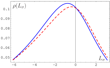
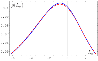
Figure 8: The dashed red line corresponds on the left panel to the first running-coupling iteration, entering the spectral density, $\rho^{\text{(2)-it-1}}_{1}(L_{\sigma})$, see Eqs. (B12)–(B14) in BMS05 , and, on the right panel, to the second running-coupling iteration, $\rho^{\text{(2)-it-2}}_{\nu=1}(L_{\sigma})$, while the solid blue line on both panels corresponds to the exact spectral density $\rho^{(2)}_{1}(L_{\sigma})$, see Eq. (105). For the sake of a better comparison, the displayed region of $L_{\sigma}$ is chosen in the vicinity of the maximum difference of these two curves.

Specifically, one can use the symbolic program Mathematica, or Maple 7, which both recognize the Lambert function, to carry out these integrations using the spectral density Mag05

$$\rho^{(2)}_{m}(\sigma)=\frac{1}{\pi}\,\textbf{Im}\left[\frac{-1}{c_{1}\,\left(1+W_{-1}(z_{\sigma})\right)}\right]^{m},$$ (105)

where $z_{\sigma}=c_{1}^{-1}\exp\left(\displaystyle-L_{\sigma}/c_{1}-1+i\pi\right)$. We present the approximate expression $\rho^{\text{(2)it-2}}_{1}(L_{\sigma})$ (dashed red line) in comparison with the exact expression $\rho^{(2)}_{1}(L_{\sigma})$ (solid blue line) in Fig. 8.

2. It is worth noting here that explicit expressions for the analytic images of the integer powers of the couplings in the Minkowski region

$${\mathfrak{A}}_{n}^{(2)}\left(L_{s}\right) = \int_{L_{s}}^{\infty}\!\!\rho^{(2)}_{n}(\sigma)dL_{\sigma}$$ (106)

have been obtained before by Magradze Mag05 , using the properties of the Lambert function; notably,

$${\mathfrak{A}}_{1}^{(2)}\left(L_{s}\right) = 1-\frac{1}{\pi}\,\textbf{Im}\,\left[\ln{W_{1}(z_{s})}\right]\,;$$ (107)

$${\mathfrak{A}}_{2}^{(2)}\left[L_{s}\right] = \frac{1}{c_{1}\pi}\,\textbf{Im}\,\left[\ln\left(\frac{W_{1}\left(z_{s}\right)}{1+W_{1}\left(z_{s}\right)}\right)\right]\,;$$ (108)

$${\mathfrak{A}}_{n+2}^{(2)}\left(L_{s}\right) = -\,\frac{1}{c_{1}}\,\left[{\mathfrak{A}}_{n+1}^{(2)}\left(L_{s}\right)+{1\over n}\,\frac{\mathrm{d}\phantom{L_{s}\!\!\!}}{\mathrm{d}L_{s}\!}\ {\mathfrak{A}}_{n}^{(2)}\left(L_{s}\right)\right]\,\text{~{}for~{}}n\geq 1\,.$$ (109)

3. For the Pade-modification of the three-loop approximation the corresponding spectral densities are defined through Eq. (97)

$$\rho^{(3\text{-P})}_{m}(\sigma)=\frac{1}{\pi}\,\textbf{Im}\left[\frac{-1}{c_{1}\,\left(1-c_{2}/c_{1}^{2}+W_{-1}\big{(}z^{(3\text{-P})}(L_{\sigma})\big{)}\right)}\right]^{m}\,.$$ (110)

The following explicit expression for the analytic image of the coupling in the Minkowski region

$${\mathfrak{A}}_{1}^{(3\text{-P})}\left(L_{s}\right)=\frac{1}{\pi}\left\{\pi-\frac{c_{1}^{2}}{c_{1}^{2}-c_{2}}\,\textbf{Im}\left[\ln{W_{1}\left(z_{s}\right)\vphantom{\frac{c_{2}}{c_{1}^{2}}}}\right]+\frac{c_{2}}{c_{1}^{2}-c_{2}}\,\textbf{Im}\left[\ln\left(1-\frac{c_{2}}{c_{1}^{2}}+W_{1}\left(z_{s}\right)\right)\right]\right\}~{}~{}~{}~{}$$ (111)

with $z_{s}=z^{(3\text{-P})}(L_{s})$ has been obtained before by Magradze Mag00 . The relative accuracy of this solution, as compared with the numerical integration of the original, non-Pade-modified, spectral density $\rho^{(3)}_{1}(\sigma)$ is better than $0.25\%$ for $L\geq 2$.

4. A useful formula to relate arbitrary powers of logarithms by means of the dispersion relation (8) has been presented in BKM01 ; viz.,

$$Q^{2}\int_{0}^{\infty}{ds\over(s+Q^{2})^{2}}\left({\mu^{2}\over s}\right)^{\delta}={\pi\delta\over\sin(\pi\delta)}\left({\mu^{2}\over Q^{2}}\right)^{\delta}\,.$$ (112)

Appendix C “Analytization” of powers of the coupling multiplied by logarithms

1. Here we derive the “analytization” of powers, $\left(a_{(2)}\right)^{\nu}$, and more complicated expressions that contain powers of the running coupling multiplied by logarithms, making use of the property

$$\left[a^{\nu}\ln(a)\right]_{\text{an}} \equiv \left[\frac{d}{d\nu}a^{\nu}\right]_{\text{an}}\,\stackrel{{\scriptstyle def}}{{=}}\,\frac{d}{d\nu}\,{\cal A}_{\nu}\,=\,{\cal D}\,{\cal A}_{\nu}\,,$$ (113)

supplemented by Eqs. (88) and (89). In this way we obtain ($c_{1}\equiv b_{1}/b_{0}^{2},~{}c_{2}\equiv b_{2}/b_{0}^{3}$)

$${{\cal A}_{\nu}^{(3)}\choose{\mathfrak{A}}_{\nu}^{(3)}}={{\cal A}_{\nu}^{(1)}\choose{\mathfrak{A}}_{\nu}^{(1)}}+c_{1}\,\nu\,{\cal D}\,{{\cal A}_{\nu+1}^{(1)}\choose{\mathfrak{A}}_{\nu+1}^{(1)}}+\nu\left[c_{1}^{2}\,\left(\frac{\nu+1}{2!}\,{\cal D}^{2}+{\cal D}-1\right)+c_{2}\right]{{\cal A}_{\nu+2}^{(1)}\choose{\mathfrak{A}}_{\nu+2}^{(1)}}~{}~{}~{}~{}~{}~{}~{}~{}$$ (114a)

$$+\,c_{1}\nu\left\{c_{1}^{2}\left[\frac{(\nu+1)(\nu+2)}{3!}\,{\cal D}^{3}+\frac{2\,\nu+3}{2}\,{\cal D}^{2}+(\nu+1)\,{\cal D}-\frac{1}{2}\right]+c_{2}(\nu+2)\,{\cal D}\right\}{{\cal A}_{\nu+3}^{(1)}\choose{\mathfrak{A}}_{\nu+3}^{(1)}}~{}~{}~{}~{}~{}$$ (114b)

$$+\nu\left\{c_{1}^{4}\left[\frac{(\nu+1)(\nu+2)(\nu+3)}{4!}\,{\cal D}^{4}+\frac{3\,\nu^{2}+12\,\nu+11}{6}\,{\cal D}^{3}-\frac{\nu^{2}+2\,\nu}{2}\,{\cal D}^{2}-\frac{3\,\nu+5}{2}\,{\cal D}\right.\right.~{}~{}~{}~{}~{}~{}\$$

$$\left.\left.+\frac{3\,\nu+4}{6}\right]+\,c_{1}^{2}c_{2}\,(\nu+2)\left[\frac{\nu+3}{2}\,{\cal D}^{2}+{\cal D}-1\right]+c_{2}^{2}\,\frac{(\nu+4)(3\nu+7)}{6}\right\}{{\cal A}_{\nu+4}^{(1)}\choose{\mathfrak{A}}_{\nu+4}^{(1)}}~{}~{}~{}~{}~{}$$ (114c)

$$+\,{\cal O}\left({\cal D}^{5}\,{{\cal A}_{\nu+4}^{(1)}\choose{\mathfrak{A}}_{\nu+5}^{(1)}}\right)\,.~{}~{}~{}~{}~{}~{}~{}~{}~{}~{}~{}~{}~{}~{}~{}~{}~{}~{}~{}~{}~{}~{}~{}~{}~{}~{}~{}~{}~{}~{}~{}~{}~{}~{}~{}~{}~{}~{}~{}~{}~{}~{}~{}~{}~{}~{}~{}~{}~{}~{}~{}~{}~{}~{}~{}~{}~{}~{}~{}~{}~{}~{}~{}~{}~{}~{}~{}~{}~{}~{}~{}~{}~{}~{}~{}~{}$$

2. The images of the coupling accompanied by logarithms of the momentum, i.e., $\left(a_{(2)}\right)^{\nu}L$, in accordance with Eq. (91), are

$${{\cal L}_{\nu}\choose{\mathfrak{L}}_{\nu}}\equiv{\textbf{A}_{\text{E}}\choose\textbf{A}_{\text{M}}}\left[\left(a_{(2)}\right)^{\nu}L\right] = {{\cal A}_{\nu-1}^{(2)}\choose{\mathfrak{A}}_{\nu-1}^{(2)}}+c_{1}\,{\cal D}\,{{\cal A}_{\nu}^{(2)}\choose{\mathfrak{A}}_{\nu}^{(2)}}-c_{1}^{2}\,{{\cal A}_{\nu+1}^{(2)}\choose{\mathfrak{A}}_{\nu+1}^{(2)}}+\frac{c_{1}^{3}}{2}\,{{\cal A}_{\nu+2}^{(2)}\choose{\mathfrak{A}}_{\nu+2}^{(2)}}$$ (115)

$$+ {\cal O}\left({\cal A}_{\nu+3}^{(2)}\right)\,.$$

Following Eq. (93), this leads to

$${{\cal L}_{\nu}^{(3)}\choose{\mathfrak{L}}_{\nu}^{(3)}}={{\cal A}_{\nu-1}^{(1)}\choose{\mathfrak{A}}_{\nu-1}^{(1)}}+c_{1}\,\nu~{}{\cal D}\,{{\cal A}_{\nu}^{(1)}\choose{\mathfrak{A}}_{\nu}^{(1)}}+\nu\left[c_{1}^{2}\,\left(\frac{\nu+1}{2!}\,{\cal D}^{2}+{\cal D}-1\right)+c_{2}\right]{{\cal A}_{\nu+1}^{(1)}\choose{\mathfrak{A}}_{\nu+1}^{(1)}}~{}~{}~{}~{}~{}~{}~{}~{}~{}$$

$$+\,c_{1}\,\nu\left\{c_{1}^{2}\left[\frac{(\nu+1)(\nu+2)}{3!}\,{\cal D}^{3}+\frac{2\,\nu+3}{2}\,{\cal D}^{2}+(\nu+1)\,{\cal D}-\frac{1}{2}\right]+c_{2}(\nu+2)\,{\cal D}\right\}{{\cal A}_{\nu+2}^{(1)}\choose{\mathfrak{A}}_{\nu+2}^{(1)}}$$

$$+\,{\cal O}\left({\cal D}^{3}{{\cal A}_{\nu+3}^{(1)}\choose{\mathfrak{A}}_{\nu+3}^{(1)}}\right)\,.~{}~{}~{}~{}~{}~{}~{}~{}~{}~{}~{}~{}~{}~{}~{}~{}~{}~{}~{}~{}~{}~{}~{}~{}~{}~{}~{}~{}~{}~{}~{}~{}~{}~{}~{}~{}~{}~{}~{}~{}~{}~{}~{}~{}~{}~{}~{}~{}~{}~{}~{}~{}~{}~{}~{}~{}~{}~{}~{}~{}~{}~{}~{}~{}~{}~{}~{}~{}~{}~{}~{}~{}~{}~{}~{}~{}~{}~{}~{}~{}~{}~{}~{}$$ (116)

Appendix D Representation of the D-function

1. The first three coefficients $d_{1},d_{2},d_{3}$ for the $D_{\text{S}}$ function of two scalar quark currents,

$$D_{\text{S}}(Q^{2}) = 3\,m_{b}^{2}(Q^{2})\left[1+\sum_{n>0}d_{n}\left({\alpha_{s}(Q^{2})\over\pi}\right)^{n}\right]\,,$$ (117)

have been calculated in Che96 and read

$$d_{1} = C_{\text{F}}\left[\frac{17}{4}\right]\,,$$ (118a)

$$d_{2} = C_{\text{F}}^{2}\left[\frac{691}{64}-\frac{9}{4}\,\zeta(3)\right]+\,C_{\text{F}}\,C_{\text{A}}\left[\frac{893}{64}-\frac{31}{8}\,\zeta(3)\right]+\,T_{\text{R}}\,N_{f}\,C_{\text{F}}\left[-\frac{65}{16}+\zeta(3)\right]\,,~{}~{}$$ (118b)

$$d_{3} = C_{\text{F}}^{3}\left[\frac{23443}{768}-\frac{239}{16}\,\zeta(3)+\frac{45}{8}\,\zeta(5)\right]+\,C_{\text{F}}^{2}\,C_{\text{A}}\left[\frac{13153}{192}-\frac{1089}{32}\,\zeta(3)+\frac{145}{16}\,\zeta(5)\right]$$ (118c)

$$+ C_{\text{F}}\,C_{\text{A}}^{2}\left[\frac{3894493}{62208}-\frac{2329}{96}\,\zeta(3)+\frac{25}{48}\,\zeta(5)\right]$$

$$+ T_{\text{R}}\,N_{f}\,C_{\text{F}}^{2}\left[-\frac{88}{3}+\frac{65}{4}\,\zeta(3)+\frac{3}{4}\,\zeta(4)-5\,\zeta(5)\right]$$

$$+ T_{\text{R}}\,N_{f}\,C_{\text{F}}\,C_{\text{A}}\left[-\frac{33475}{972}+\frac{22}{3}\,\zeta(3)-\frac{3}{4}\,\zeta(4)+\frac{5}{6}\,\zeta(5)\right]$$

$$+ T_{\text{R}}^{2}\,N_{f}^{2}\,C_{\text{F}}\left[\frac{15511}{3888}-\zeta(3)\right]\,.$$

The result for $$d_{4}$$ was obtained quite recently in BCK05 ,

$$d_{4} = N_{f}^{3}\left[-\frac{520771}{559872}+\frac{65}{432}\,\zeta(3)+\frac{1}{144}\,\zeta(4)+\frac{5}{18}\,\zeta(5)\right]$$ (118d)

$$+ N_{f}^{2}\left[\frac{220313525}{2239488}-\frac{11875}{432}\,\zeta(3)+\frac{5}{6}\,\zeta^{2}(3)+\frac{25}{96}\,\zeta(4)-\frac{5015}{432}\,\zeta(5)\right]$$

$$+ N_{f}\left[-\frac{1045811915}{373248}+\frac{5747185}{5184}\,\zeta(3)-\frac{955}{16}\,\zeta^{2}(3)-\frac{9131}{576}\,\zeta(4)+\frac{41215}{432}\,\zeta(5)\right.$$

$$\phantom{N_{f}^{0}}\left.~{}+\frac{2875}{288}\,\zeta(6)+\frac{665}{72}\,\zeta(7)\right]$$

$$+ N_{f}^{0}\left[\frac{10811054729}{497664}-\frac{3887351}{324}\,\zeta(3)+\frac{458425}{432}\,\zeta^{2}(3)+\frac{265}{18}\,\zeta(4)+\frac{373975}{432}\,\zeta(5)\right.$$

$$\phantom{N_{f}^{0}}\left.~{}-\frac{1375}{32}\,\zeta(6)-\frac{178045}{768}\,\zeta(7)\right]\,.$$

2. The coefficients $\gamma_{i}$ determine the expansion of the quark-mass anomalous dimension in analogous manner as Eq. (82) does with respect to the expansion of the $\beta$-function; viz.,

$$\frac{d}{dL}\ln\left(m(L)\right)=-\sum_{i\geq 0}\gamma_{i}\left(\frac{\alpha_{s}(L)}{4\pi}\right)^{i+1},$$ (119)

with the following expressions, see Che97 ,

$$\gamma_{0} = 3C_{\text{F}}\,;$$ (120)

$$\gamma_{1} = \bigg{[}\frac{202}{3}-\frac{20}{9}\,N_{f}\bigg{]}\,;$$ (121)

$$\gamma_{2} = \bigg{[}1249-\bigg{(}\frac{2216}{27}+\frac{160}{3}\zeta(3)\bigg{)}\,N_{f}-\frac{140}{81}\,N_{f}^{2}\bigg{]}\,;$$ (122)

$$\gamma_{3} = \bigg{[}\frac{4603055}{162}+\frac{135680}{27}\zeta(3)-8800\zeta(5)$$ (123)

$${}-\bigg{(}\frac{91723}{27}+\frac{34192}{9}\zeta(3)-880\zeta(4)-\frac{18400}{9}\zeta(5)\bigg{)}\,N_{f}$$

$${}+\bigg{(}\frac{5242}{243}+\frac{800}{9}\zeta(5)-\frac{160}{3}\zeta(4)\bigg{)}\,N_{f}^{2}-\bigg{(}\frac{332}{243}-\frac{64}{27}\zeta(3)\bigg{)}\,N_{f}^{3}\bigg{]}\,,$$

where $\zeta(\nu)$ denotes the Riemann $\zeta$ function.

References

• (1) A. P. Bakulev, S. V. Mikhailov, and N. G. Stefanis, Phys. Rev. D72, 074014 (2005); Phys. Rev. D72, 119908(E) (2005).
• (2) M. R. Pennington and G. G. Ross, Phys. Lett. B102, 167 (1981).
• (3) M. R. Pennington, R. G. Roberts, and G. G. Ross, Nucl. Phys. B242, 69 (1984).
• (4) R. Marshall, Z. Phys. C43, 595 (1989).
• (5) J. M. Cornwall, Phys. Rev. D26, 1453 (1982).
• (6) G. Parisi and R. Petronzio, Nucl. Phys. B154, 427 (1979).
• (7) M. B. Gay Ducati, F. Halzen, and A. A. Natale, Phys. Rev. D48, 2324 (1993).
• (8) A. C. Mattingly and P. M. Stevenson, Phys. Rev. Lett. 69, 1320 (1992).
• (9) N. G. Stefanis, Eur. Phys. J. direct C7, 1 (1999) [hep-ph/9911375].
• (10) A. V. Radyushkin, Dubna Preprint JINR-E2-82-159, Feb 1982; JINR Rapid Commun. 4[78], 96 (1996) [hep-ph/9907228].
• (11) N. V. Krasnikov and A. A. Pivovarov, Phys. Lett. B116, 168 (1982).
• (12) D. V. Shirkov, Theor. Math. Phys. 127, 409 (2001).
• (13) A. P. Bakulev, A. V. Radyushkin, and N. G. Stefanis, Phys. Rev. D62, 113001 (2000).
• (14) D. V. Shirkov, Eur. Phys. J. C22, 331 (2001).
• (15) M. Beneke and V. M. Braun, Phys. Lett. B348, 513 (1995).
• (16) P. Ball, M. Beneke, and V. M. Braun, Nucl. Phys. B452, 563 (1995).
• (17) D. V. Shirkov and I. L. Solovtsov, JINR Rapid Commun. 2[76], 5 (1996).
• (18) D. V. Shirkov and I. L. Solovtsov, Phys. Rev. Lett. 79, 1209 (1997).
• (19) K. A. Milton and I. L. Solovtsov, Phys. Rev. D55, 5295 (1997).
• (20) K. A. Milton and O. P. Solovtsova, Phys. Rev. D57, 5402 (1998).
• (21) I. L. Solovtsov and D. V. Shirkov, Phys. Lett. B442, 344 (1998).
• (22) B. A. Magradze, Int. J. Mod. Phys. A15, 2715 (2000).
• (23) B. A. Magradze, Dubna preprint E2-2000-222, 2000 [hep-ph/0010070] (unpublished).
• (24) D. S. Kourashev and B. A. Magradze, Preprint RMI-2001-18, 2001 [hep-ph/0104142] (unpublished).
• (25) B. A. Magradze, Preprint RMI-2003-55, 2003 [hep-ph/0305020] (unpublished).
• (26) D. S. Kourashev and B. A. Magradze, Theor. Math. Phys. 135, 531 (2003) [Teor. Mat. Fiz. 135, 95 (2003)].
• (27) B. A. Magradze, Few Body Syst. 40, 71 (2006).
• (28) H. F. Jones and I. L. Solovtsov, Phys. Lett. B349, 519 (1995).
• (29) K. A. Milton, I. L. Solovtsov, and O. P. Solovtsova, Phys. Lett. B415, 104 (1997).
• (30) K. A. Milton, I. L. Solovtsov, O. P. Solovtsova, and V. I. Yasnov, Eur. Phys. J. C14, 495 (2000).
• (31) K. A. Milton, I. L. Solovtsov, and O. P. Solovtsova, Phys. Lett. B439, 421 (1998).
• (32) K. A. Milton, I. L. Solovtsov, and O. P. Solovtsova, Phys. Rev. D60, 016001 (1999).
• (33) D. V. Shirkov and A. V. Zayakin, hep-ph/0512325 (unpublished).
• (34) N. G. Stefanis, W. Schroers, and H.-C. Kim, Phys. Lett. B449, 299 (1999).
• (35) N. G. Stefanis, W. Schroers, and H.-C. Kim, Eur. Phys. J. C18, 137 (2000).
• (36) A. P. Bakulev, K. Passek-Kumerički, W. Schroers, and N. G. Stefanis, Phys. Rev. D70, 033014 (2004); A. P. Bakulev, K. Passek-Kumerički, W. Schroers, and N. G. Stefanis, Phys. Rev. D70, 079906(E) (2004).
• (37) I. L. Solovtsov and D. V. Shirkov, Theor. Math. Phys. 120, 1220 (1999).
• (38) D. V. Shirkov and I. L. Solovtsov, hep-ph/0611229.
• (39) B. V. Geshkenbein, B. L. Ioffe, and K. N. Zyablyuk, Phys. Rev. D64, 093009 (2001).
• (40) A. A. Pivovarov, Z. Phys. C53, 461 (1992).
• (41) F. Le Diberder and A. Pich, Phys. Lett. B289, 165 (1992).
• (42) Y. L. Dokshitzer, G. Marchesini, and B. R. Webber, Nucl. Phys. B469, 93 (1996).
• (43) Y. L. Dokshitzer, in 29th International Conference On High-Energy Physics (ICHEP 98), 23–29 Jul 1998, Vancouver, British Columbia, Canada, edited by A. Astbury, D. Axen, and J. Robinson (World Scientific, Singapore, (1999), Vol. 1, pp. 305–324 [hep-ph/9812252].
• (44) S. Catani, M. L. Mangano, P. Nason, and L. Trentadue, Nucl. Phys. B478, 273 (1996).
• (45) G. Grunberg, Preprint CPTH-S505-0597, 1997 [hep-ph/9705290] (unpublished).
• (46) E. Gardi, G. Grunberg, and M. Karliner, JHEP 07, 007 (1998).
• (47) L. Magnea, Nucl. Phys. B593, 269 (2001).
• (48) A. A. Pivovarov, Phys. Atom. Nucl. 66, 724 (2003).
• (49) S. Groote, J. G. Körner, and A. A. Pivovarov, Phys. Rev. D65, 036001 (2002).
• (50) A. V. Nesterenko, Int. J. Mod. Phys. A18, 5475 (2003).
• (51) A. I. Alekseev, Few-Body Syst. 40, 57 (2006).
• (52) G. Cvetič and C. Valenzuela, J. Phys. G32, L27 (2006).
• (53) P. A. Ra̧zka, Preprint IFT-16-2005, 2005 [hep-ph/0602085] (unpublished).
• (54) A. V. Nesterenko and J. Papavassiliou, Phys. Rev. D71, 016009 (2005).
• (55) F. M. Dittes and A. V. Radyushkin, Sov. J. Nucl. Phys. 34, 293 (1981) [Yad. Fiz. 34, 529 (1981)].
• (56) E. Braaten and S.-M. Tse, Phys. Rev. D35, 2255 (1987).
• (57) D. Müller, Phys. Rev. D59, 116003 (1999).
• (58) B. Melić, B. Nižić, and K. Passek, Phys. Rev. D60, 074004 (1999).
• (59) B. Melić, B. Nižić, and K. Passek, Phys. Rev. D65, 053020 (2002).
• (60) B. Melić, D. Müller, and K. Passek-Kumerički, Phys. Rev. D68, 014013 (2003).
• (61) A. I. Karanikas and N. G. Stefanis, Phys. Lett. B504, 225 (2001); A. I. Karanikas and N. G. Stefanis, Phys. Lett. B636, 330(E) (2006).
• (62) N. G. Stefanis, Lect. Notes Phys. 616, 153 (2003) [hep-ph/0203103].
• (63) D. J. Broadhurst, A. L. Kataev, and C. J. Maxwell, Nucl. Phys. B592, 247 (2001).
• (64) N. N. Bogolyubov, A. A. Logunov, and D. V. Shirkov, Soviet Physics JETP 37, 574 (1960).
• (65) R. Oehme, Phys. Lett. B252, 641 (1990).
• (66) N. G. Stefanis, A. P. Bakulev, A. I. Karanikas, and S. V. Mikhailov, plenary talk at 2nd Workshop on Hadron Structure and QCD: From Low to High Energy (HSQCD 2005), St. Petersburg, Russia, 20–24 Sep 2005, to be published in the proceedings [hep-ph/0601270].
• (67) A. P. Bakulev, A. I. Karanikas, and N. G. Stefanis, Phys. Rev. D72, 074015 (2005).
• (68) N. G. Stefanis et al., in First International Workshop “Hadron Structure and QCD (HSQCD 2004): From Low to High Energies”, Repino, St. Petersburg, Russia, 18–22 May 2004, edited by V. T. Kim and L. N. Lipatov (PNPI, Gatchina, St. Petersburg, 2004), pp. 238–245 [hep-ph/0409176].
• (69) N. G. Stefanis, Nucl. Phys. Proc. Suppl. 152, 245 (2006), invited talk given at 11th International Conference in Quantum ChromoDynamics (QCD 04), Montpellier, France, 5–9 Jul 2004.
• (70) A. P. Bakulev, in Proceedings of the 13th International Seminar Quarks’2004, Vol. 2, Pushkinogorie, Russia, May 24–30, 2004, edited by D. G. Levkov, V. A. Matveev, and V. A. Rubakov (INR RAS, Moscow, 2005), pp. 536–550 [hep-ph/0410134].
• (71) A. P. Bakulev, in QUARK CONFINEMENT AND THE HADRON SPECTRUM VI, 6th Conference on Quark Confinement and the Hadron Spectrum, QCHS 2004, Villasimius, Italy, 21–25 September 2004, AIP Conf. Proc. No. 756 (AIP, New York, 2005), pp. 342–344 [hep-ph/0412248].
• (72) K. G. Chetyrkin, Phys. Lett. B390, 309 (1997).
• (73) K. G. Chetyrkin, B. A. Kniehl, and A. Sirlin, Phys. Lett. B402, 359 (1997).
• (74) P. A. Baikov, K. G. Chetyrkin, and J. H. Kühn, Phys. Rev. Lett. 96, 012003 (2006).
• (75) D. V. Shirkov, Theor. Math. Phys. 119, 438 (1999).
• (76) D. V. Shirkov, Dubna preprint E2-2000-211, 2000 [hep-ph/0009106] (unpublished).
• (77) D. V. Shirkov, AIP Conf. Proc. 806, 97 (2006) [hep-ph/0510247].
• (78) H. Batemann and A. Erdelýi, Higher transcendental functions (Batemann Manuscript Project) (McGraw-Hill, New York, 1953).
• (79) A. Djouadi, Preprint LPT-ORSAY-05-17, 2005 [hep-ph/0503172] (unpublished).
• (80) J. G. Körner, F. Krajewski, and A. A. Pivovarov, Eur. Phys. J. C20, 259 (2001).
• (81) K. G. Chetyrkin, Phys. Lett. B404, 161 (1997).
• (82) A. L. Kataev, G. Parente, and A. V. Sidorov, Phys. Part. Nucl. 34, 20 (2003).
• (83) R. Corless et al., Advances in Computation Mathematics 5, 329 (1996).