Semi-inclusive hadronic $B$ decays in the endpoint region

Abstract

We consider in the soft-collinear effective theory semi-inclusive hadronic $B$ decays, $B\rightarrow XM$, in which an energetic light meson $M$ near the endpoint recoils against an inclusive jet $X$. We focus on a subset of decays where the spectator quark from the $B$ meson ends up in the jet. The branching ratios and direct CP asymmetries are computed to next-to-leading order accuracy in $\alpha_{s}$ and to leading order in $1/m_{b}$. The contribution of charming penguins is extensively discussed, and a method to extract it in semi-inclusive decays is suggested. Subleading $1/m_{b}$ corrections and $SU(3)$ breaking effects are discussed.

I Introduction

Semi-inclusive hadronic decays $B\to XM$ have received much less attention over the years in contrast to the widely studied exclusive two-body $B$ decays Cheng:2001nj ; Atwood:1997de ; Browder:1997yq ; Soni:2005jj ; Eilam:2002wu ; Kagan:1997qn ; He:1998se ; Kim:2002gv ; Calmet:1999ix . As we will show in this paper, semi-inclusive hadronic $B$ decays in the endpoint region, where $M$ is an isolated energetic meson and $X$ is a collinear jet of hadrons in the opposite direction, are theoretically simpler than the exclusive two-body $B$ decays in many respects, yet still address many of the questions that had been debated in the context of the two-body $B$ decays. Using the soft-collinear effective theory (SCET) Bauer:2000ew ; Bauer:2000yr ; Bauer:2001ct ; Bauer:2001yt predictions of semi-inclusive decays can be improved systematically and lead to the following advantages. Firstly, larger data samples can be included by considering inclusive jets with a variety of final-state particles forming the collinear jet. Secondly, as in exclusive $B$ decays Chay:2003ju ; Chay:2003zp , the four-quark operators in the weak Hamiltonian factorize at leading order in $1/m_{b}$ into a product of a heavy-to-light current and a collinear current, with no strong interactions between these two currents. Thirdly, the inclusive collinear jet is described by the jet function, which is obtained by matching the full theory onto $\mathrm{SCET}_{\mathrm{I}}$ at the scale $p_{X}^{2}\sim m_{b}\Lambda$ with $\Lambda\sim\Lambda_{\mathrm{QCD}}$. Since the same jet function appears at leading order in $B\to X_{s}\gamma$ or $B\to Xl\overline{\nu}$ inclusive decays, many of the hadronic uncertainties cancel by taking ratios. Finally, the contribution of charming penguins can be implemented systematically using the effective theory. Studying $B\rightarrow XM$ decays can thus offer a theoretical handle to probe nonperturbative effects of charming penguins.

In order to see these advantages clearly, we consider the decays $B\rightarrow XM$ in which the spectator quark of the $B$ meson goes to the inclusive jet. It is straightforward to treat other decay modes without this constraint work , but would involve more calculation including spectator interactions, and we do not discuss it further here. The decay rate for $B\to XM$ at leading order in $1/m_{b}$ can then be schematically written as

$$\frac{d\Gamma}{dE_{M}}\sim\big{(}|\mathcal{T}\otimes\phi_{M}|^{2}\big{)}\cdot\big{(}\mathcal{J}\otimes f\big{)},$$ (1)

where $\mathcal{T}$ is a collection of hard coefficients obtained in matching full QCD onto SCET_I and $\mathcal{J}$ is the discontinuity of the jet function describing the fluctuations of order $m_{b}\Lambda$ in the forward scattering amplitude of the heavy-to-light currents. $\phi_{M}$ and $f$ are the light-cone distribution amplitude (LCDA) for the light meson $M$ and the $B$-meson shape function, respectively. The $\otimes$ sign implies the appropriate convolution. The convolution $\mathcal{J}\otimes f$ in Eq. (1) is universal in the sense that the same convolution appears in $B\to X_{s}\gamma$ and $B\to X_{u}l\overline{\nu}$ decays Bauer:2000ew ; Bauer:2003pi . Therefore, if we take the ratios of the decay rates for $B\to XM$ and, say, the decay rate for $B\to X_{s}\gamma$, this convolution cancels out and the only surviving nonperturbative parameters are the LCDAs.

Another interesting but complicated problem common to two-body $B$ decays and $B\rightarrow XM$ decays in the endpoint region is the contribution of intermediate charming penguins, which can be of nonperturbative nature Ciuchini . There has been a disagreement on how to treat this contribution between the recent SCET analysis of the two-body $B$ decays Bauer:2004tj ; Williamson:2006hb and the approach of QCD factorization Beneke:1999br . The question is whether or not the long-distance effects of charming penguins are of leading order in $1/m_{b}$. Long-distance contributions arise when intermediate charm quarks lie in the non-relativistic QCD (NRQCD) regime with small relative velocity $v^{*}$. These contributions are of the form $\alpha_{s}(2m_{c})f(2m_{c}/m_{b})v^{*}$ Bauer:2005wb , where $f(2m_{c}/m_{b})$ is a factor which accounts for the phase space in which the charm quarks have small relative velocities. In QCD factorization Beneke:1999br ; Beneke:2004bn , the claim is that the phase space suppression near the threshold region is strong enough so that the nonperturbative contributions are subleading. On the other hand, Bauer et al. Bauer:2004tj ; Bauer:2005wb argue that since $2m_{c}/m_{b}$ is of order unity so is $f(2m_{c}/m_{b})$, and the nonperturbative contribution of charming penguins can be of leading order. In this paper, we suggest how to resolve the issue of charming penguins in $B\rightarrow XM$ decays. If the nonperturbative contributions of charming penguins are really suppressed, then the decay rates at leading order in $1/m_{b}$ are completely determined in terms of the perturbatively calculable hard kernels convoluted with LCDA, once normalized to the $B\to X_{s}\gamma$ rate. If nonperturbative charming penguins are not suppressed, they will show up experimentally as a sizable deviation from purely perturbative predictions, which we will discuss in detail.

The paper is organized as follows: In Section II we describe the kinematics for $B\rightarrow MX$ decays. In Section III, we set up the operator basis for the decays $B\rightarrow MX$ and compute the radiative corrections at next-to-leading order (NLO) to derive the renormalization group equations for the operators. In Section IV, we present a factorized form for the semi-inclusive $B$ decays in the endpoint region. Section V is devoted to the contribution of charming penguins, considering two possible scenarios in which the charm quark is regarded as either hard-collinear or heavy. The contribution of charming penguins in the heavy quark limit $m_{b},m_{c}\rightarrow\infty$ with $m_{c}/m_{b}$ fixed is considered in detail. In Section VI, we discuss the corrections to the leading order prediction, including $SU(3)$ breaking effects. In Section VII, we perform the phenomenological analysis of $B\rightarrow MX$ decays and predict the decay rates and CP asymmetries. The method to extract the effect of charming penguins is also discussed. We conclude in Section VIII. In Appendix A we present the Wilson coefficients for the operators at NLO in $\mathrm{SCET}_{\rm I}$. In Appendix B the detailed analysis of charming penguins in the heavy quark limit is discussed.

II Kinematics

Using SCET, solid predictions can be made for hadronic semi-inclusive $B\to MX$ decays in the endpoint region. In the rest frame of the $B$ meson, the outgoing energetic meson $M$ with $p_{M}^{2}\sim\Lambda^{2}$ moves in the $\overline{n}^{\mu}$ direction, while the inclusive hard-collinear jet with $p_{X}^{2}\sim\Lambda m_{b}$ is in the $n^{\mu}$ direction, where $n^{2}=\overline{n}^{2}=0$, $n\cdot\overline{n}=2$. We can choose the reference frame in which the transverse momentum of $M$ is zero. The momenta $p_{M}^{\mu}$ and $p_{X}^{\mu}$ can be written in terms of the light-cone coordinates $p^{\mu}=(\overline{n}\cdot p,n\cdot p,p_{\perp})$ as

$$p_{M} = \left(0,n\cdot p_{M},\vec{0}\right)+{\cal O}(\Lambda^{2}/m_{B}),$$

$$p_{X} = \left(m_{B},m_{B}-n\cdot p_{M},\vec{0}\right)+{\cal O}(\Lambda^{2}/m_{B}),$$ (2)

with $p_{B}^{\mu}=m_{B}v^{\mu}=p_{M}^{\mu}+p_{X}^{\mu}$, where $2v^{\mu}=n^{\mu}+\overline{n}^{\mu}$. We consider the endpoint region in which $m_{B}-n\cdot p_{M}\sim\Lambda$, so that $p_{X}^{2}\sim m_{B}\Lambda$.

At the quark level, the $b$ quark has momentum $p_{b}^{\mu}=m_{b}v^{\mu}+l^{\mu}$, where $l^{\mu}$ is the residual momentum of order $\Lambda_{\rm QCD}$. The $b$ quark decays to a quark–antiquark pair moving in the $\overline{n}$ direction which hadronizes into the meson $M$, and another quark with momentum $p_{J}^{\mu}$ moving in the $n$ direction, which combines with a spectator antiquark to form the outgoing jet $X$. The momentum $p_{J}^{\mu}$ can be written as (dropping terms of order $\Lambda^{2}/m_{b}$)

$$p_{J}^{\mu}=m_{b}v^{\mu}+l^{\mu}-p_{M}^{\mu}=m_{b}\frac{n^{\mu}}{2}+m_{b}(1-x_{M})\frac{\overline{n}^{\mu}}{2}+l^{\mu}=m_{b}\frac{n^{\mu}}{2}+k^{\mu},$$ (3)

where $x_{M}=n\cdot p_{M}/m_{b}=2E_{M}/m_{b}$. In the endpoint region, $1-x_{M}\sim\Lambda/m_{b}$. Since the invariant mass squared $p_{J}^{2}$ of the jet is time-like, the range of the residual momentum $k^{\mu}$ in $p_{J}^{\mu}$ is $0\leq n\cdot k\leq n\cdot p_{X}$. Since the residual momentum of the heavy quark $n\cdot l$ is smaller than $\overline{\Lambda}=m_{B}-m_{b}$, the region of $n\cdot l$, which has support for the $B$-meson shape function, is

$$-m_{b}(1-x_{M})\leq n\cdot l\leq\overline{\Lambda}.$$ (4)

III Matching and evolution in $\rm{SCET_{I}}$

We employ a two-step matching in computing and evolving the hard coefficients. First we construct the operators for the decays in $\rm{SCET_{I}}$ by integrating out degrees of freedom of order $m_{b}$. The Wilson coefficients of the operators are obtained by matching full QCD onto $\rm{SCET_{I}}$. The decay rates of the semi-inclusive $B$ decays are obtained from the forward scattering amplitude of the time-ordered product of the heavy-to-light currents, as shown in Fig. 1. In the next step, we match $\mathrm{SCET}_{\mathrm{I}}$ onto $\mathrm{SCET}_{\mathrm{II}}$ by integrating out the degrees of freedom with $p^{2}\sim m_{b}\Lambda$. As a result, the jet function is obtained, the discontinuity of which contributes to the semi-inclusive hadronic $B$ decay rates.

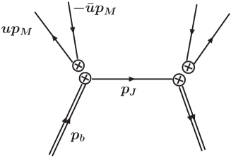
Figure 1: Tree-level diagram for the forward scattering of the heavy-to-light currents in $\rm{SCET_{I}}$ whose discontinuity gives the semi-inclusive hadronic $B$ decay rates in the endpoint region. The double lines denote a heavy quark, the intermediate line is the hard-collinear quark in the $n$ direction with $p_{J}^{2}=m_{b}^{2}(1-x_{M})$, while the upward collinear quarks move in the $\overline{n}$ direction.

The effective weak Hamiltonian in full QCD for hadronic $B$ decays is given as

$$H_{W}=\frac{G_{F}}{\sqrt{2}}\Biggl{[}\sum_{p=u,c}\lambda_{p}^{(q)}\Bigl{(}C_{1}O_{1}^{p}+C_{2}O_{2}^{p}\Bigr{)}-\lambda_{t}^{(q)}\Bigl{(}\sum_{i=3}^{10}C_{i}O_{i}+C_{g}O_{g}+C_{\gamma}O_{\gamma}\Bigr{)}\Biggr{]},$$ (5)

where the operators are

$$O_{1}^{p} =(\overline{p}b)_{V-A}(\overline{q}p)_{V-A},\qquad\qquad\qquad\quad O_{2}^{p} =(\overline{p}_{\beta}b_{\alpha})_{V-A}(\overline{q}_{\alpha}p_{\beta})_{V-A},$$ (6)

$$O_{3,5} =(\overline{q}b)_{V-A}\sum_{q^{\prime}}(\overline{q^{\prime}}q^{\prime})_{V\mp A}, O_{4,6} =(\overline{q}_{\beta}b_{\alpha})_{V-A}\sum_{q^{\prime}}(\overline{q^{\prime}}_{\alpha}q^{\prime}_{\beta})_{V\mp A},$$

$$O_{7,9} =(\overline{q}b)_{V-A}\sum_{q^{\prime}}\frac{3e_{q^{\prime}}}{2}(\overline{q^{\prime}}q^{\prime})_{V\pm A}, O_{8,10} =(\overline{q}_{\beta}b_{\alpha})_{V-A}\sum_{q^{\prime}}\frac{3e_{q^{\prime}}}{2}(\overline{q^{\prime}}_{\alpha}q^{\prime}_{\beta})_{V\pm A},$$

$$O_{\gamma} =-\frac{em_{b}}{8\pi^{2}}\overline{q}\sigma^{\mu\nu}F_{\mu\nu}(1+\gamma_{5})b, O_{g} =-\frac{gm_{b}}{8\pi^{2}}\overline{q}\sigma^{\mu\nu}G^{a}_{\mu\nu}T^{a}(1+\gamma_{5})b.$$

Here $\lambda_{p}^{(q)}=V_{pb}V_{pq}^{*}$ is the CKM factor and $V\pm A=\gamma^{\mu}(1\pm\gamma_{5})$. The summation over $q^{\prime}$ includes $u$, $d$, $s$, $c$ and $b$ quarks. Operators with $q=d$ ($q=s$) describe the $\Delta S=0$ ($\Delta S=1$) effective weak Hamiltonian.

The effective Hamiltonian in $\rm{SCET_{I}}$ at leading order (LO) in $1/m_{b}$ is (with charm quarks integrated out, nonperturbative charm contributions will be discussed in Section V) Chay:2003ju ; Bauer:2004tj

$$H_{I}=\frac{2G_{F}}{\sqrt{2}}\sum_{p=u,c}\lambda_{p}^{(q)}\sum_{i=1}^{6}\mathcal{C}_{i}^{p}\otimes{\cal O}_{i},$$ (7)

where the relevant four-quark operators are

$${\cal O}_{1} =\big{[}\overline{u}_{n}{\overline{n}}\!\!\!/P_{L}Y_{n}^{\dagger}b_{v}\big{]}\big{[}\overline{q}_{\overline{n}}{n}\!\!\!/P_{L}u_{\overline{n}}\big{]}_{u},\qquad\qquad {\cal O}_{2,3} =\big{[}\overline{q}_{n}{\overline{n}}\!\!\!/P_{L}Y_{n}^{\dagger}b_{v}\big{]}\big{[}\overline{u}_{\overline{n}}{n}\!\!\!/P_{L,R}u_{\overline{n}}\big{]}_{u},$$ (8)

$${\cal O}_{4} =\sum_{q^{\prime}}\big{[}\overline{q^{\prime}}_{n}{\overline{n}}\!\!\!/P_{L}Y_{n}^{\dagger}b_{v}\big{]}\big{[}\overline{q}_{\overline{n}}{n}\!\!\!/P_{L}q^{\prime}_{\overline{n}}\big{]}_{u}, {\cal O}_{5,6} =\sum_{q^{\prime}}\big{[}\overline{q}_{n}{\overline{n}}\!\!\!/P_{L}Y_{n}^{\dagger}b_{v}\big{]}\big{[}\overline{q^{\prime}}_{\overline{n}}{n}\!\!\!/P_{L,R}q^{\prime}_{\overline{n}}\big{]}_{u}.$$

The summation over $q^{\prime}$ includes $u$, $d$ and $s$ quarks and $P_{L,R}=(1\mp\gamma_{5})/2$. In Eq. (7), $\otimes$ denotes the convolution

$$\mathcal{C}_{i}^{p}\otimes{\cal O}_{i}=\int_{0}^{1}du~{}\mathcal{C}_{i}^{p}(u){\cal O}_{i}(u),$$ (9)

and the subscript $u$ in Eq. (8) refers to the variable in a $\delta$ function, which is defined as

$$\big{[}\overline{q}_{\overline{n}}{n}\!\!\!/P_{L}q_{\overline{n}}\big{]}_{u}\equiv\Bigl{[}\overline{q}_{\overline{n}}\;\delta\!\Big{(}u-\frac{n\cdot\mathcal{P}^{\dagger}}{2E_{M}}\Big{)}{n}\!\!\!/P_{L}q_{\overline{n}}\Bigr{]}.$$ (10)

The $q_{n}$ and $q_{\bar{n}}$ are the gauge-invariant quark fields

$$q_{n}=W_{n}^{\dagger}\xi_{n}^{(q)},\ q_{\bar{n}}=W_{\bar{n}}^{\dagger}\xi_{\bar{n}}^{(q)},$$ (11)

given in terms of the collinear fermion fields $\xi_{n}^{(q)}$, $\xi_{\bar{n}}^{(q)}$ of flavor $q$ and the collinear Wilson lines $W_{n}$, $W_{\bar{n}}$ in the $n$ and $\overline{n}$ directions, respectively. The ultrasoft (usoft) Wilson line in the $n$ direction, $Y_{n}$, is obtained after redefining the collinear fields to decouple collinear and usoft degrees of freedom Bauer:2001yt .

There are also color-octet operators corresponding to the operators in Eq. (7), e.g.,

$$\overline{\mathcal{O}}_{1}(u)=\big{[}\overline{u}_{n}Y_{n}^{\dagger}Y_{\overline{n}}{\overline{n}}\!\!\!/P_{L}T^{a}Y_{\overline{n}}^{\dagger}b_{v}\big{]}\big{[}\overline{q}_{\overline{n}}{n}\!\!\!/P_{L}T^{a}u_{\overline{n}}\big{]}_{u},$$ (12)

but the matrix elements of the octet operators between hadronic states vanish and are therefore not relevant here. The Wilson coefficients $\mathcal{C}_{i}^{p}(u)$ in Eq. (7) encode physics at the hard scale $m_{b}$ and are perturbatively calculable in powers of $\alpha_{s}(m_{b})$. They are known at NLO in $\alpha_{s}$ Beneke:1999br ; Chay:2003ju and are listed in Appendix A. Note that the Wilson coefficients $\mathcal{C}_{i}^{p}(u)$ exhibit nonzero strong phases at NLO from integrating out the intermediate on-shell quarks.

In matching $\rm{SCET_{I}}$ onto $\rm{SCET_{II}}$ at $\mu_{0}\sim\sqrt{m_{b}\Lambda}$, the operators in the Hamiltonian in Eq. (7) are first evolved down from $m_{b}$ to $\mu_{0}$ using the renormalization group (RG) equation in $\rm{SCET_{I}}$. The operators in Eq. (7) factor into a heavy-to-light current $J_{H}^{\mu}$ and a collinear current $J_{C}^{\mu}$ as

$${\cal O}(u,\mu)=\Bigl{[}\overline{q}_{n}\Gamma_{H}Y_{n}^{\dagger}b_{v}\Bigr{]}\Bigl{[}\overline{q}_{\overline{n}}\Gamma_{C}q_{\overline{n}}\Bigr{]}_{u}=J_{H}(\mu)\cdot J_{C}(u,\mu),$$ (13)

where $\Gamma_{H,C}$ are the Dirac structure in each current. There are no strong interactions between the two currents to all orders in $\alpha_{s}$ in $\rm{SCET_{I}}$. At order $\alpha_{s}$, the radiative corrections in Fig. 2 show explicitly that this is true. As a result, the operator $\cal O$ is multiplicatively renormalized, and there is no mixing between color-singlet and color-octet operators due to factorization.

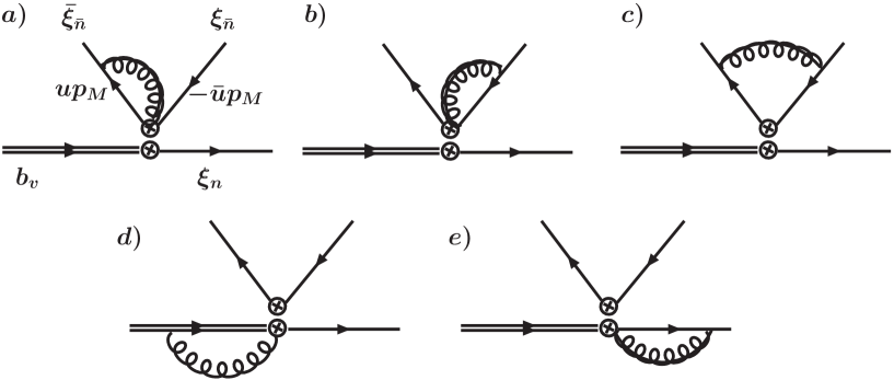
Figure 2: Feynman diagrams at order $\alpha_{s}$ for the four-quark operators in $\rm{SCET_{I}}$. Note that there is no strong interaction between the two currents.

The renormalized operator ${\cal O}_{R}$ and the bare operator ${\cal O}_{B}$ are related by

$${\cal O}_{R}(u,\mu)=\int dvZ^{-1}(u,v,\mu){\cal O}_{B}(v,\mu)=\int dvZ_{H}^{-1}(\mu)Z_{C}^{-1}(u,v,\mu){\cal O}_{B}(v,\mu),$$ (14)

where the counterterm $Z$ is a product of the counterterms $Z_{H}$ and $Z_{C}$ from the radiative corrections of $J_{H}^{\mu}$ and $J_{C}^{\mu}$. This leads to the RG equation

$$\begin{split}\mu\frac{d}{d\mu}{\cal O}(u,\mu)&=\Bigl{(}\mu\frac{d}{d\mu}J_{H}(\mu)\Bigr{)}J_{C}(u,\mu)+J_{H}(\mu)\mu\frac{d}{d\mu}J_{C}(u,\mu)\\ &=-\gamma_{H}J_{H}(\mu)J_{C}(u,\mu)-J_{H}(\mu)\int dv\gamma_{C}(u,v,\mu)J_{C}(v,\mu),\end{split}$$ (15)

whereas the RG equation for the Wilson coefficients is written as

$$\mu\frac{d}{d\mu}\mathcal{C}_{i}(u,\mu)=\int_{0}^{1}dv\Bigl{[}\gamma_{H}(\mu)\delta(u-v)+\gamma_{C}(v,u,\mu)\Bigr{]}\mathcal{C}_{i}(v,\mu).$$ (16)

At next-to-leading logarithm (NLL), the anomalous dimensions for $J_{H}$ and $J_{C}$ are given by

$$\gamma_{H}(\mu) = -\frac{\alpha_{s}C_{F}}{\pi}\ln\frac{\mu}{m_{b}}-\frac{\alpha_{s}C_{F}}{2\pi}\Bigl{(}\frac{5}{2}+\frac{\alpha_{s}}{\pi}B\ln\frac{\mu}{m_{b}}\Bigr{)},$$ (17)

$$\gamma_{C}(u,v,\mu) = -\frac{\alpha_{s}C_{F}}{2\pi}\Biggl{[}\frac{3}{2}\delta(u-v)+2\frac{u}{v}\Bigl{(}1+\frac{1}{(v-u)_{+}}\Bigr{)}\theta(v-u)+\Bigl{(}u,v\leftrightarrow\bar{u},\bar{v}\Bigr{)}\Biggl{]},$$ (18)

where $C_{F}=(N^{2}-1)/(2N)$ with $N$ the number of colors. The subscript ‘+’ denotes the plus distribution, and $\bar{u}=1-u$. The one-loop result for $\gamma_{H}$ in SCET was first obtained in Ref. Bauer:2000ew , while the part of the two-loop result containing $\alpha_{s}^{2}\ln(\mu/m_{b})$ needed at NLL accuracy has not yet been calculated in SCET. Extracting it from the full QCD calculation Korchemsky:1994jb , one gets $B=N(67/18-\pi^{2}/6)-5n_{f}/9$, where $n_{f}$ is the number of flavors. The one-loop result for $\gamma_{C}$ can be taken from the full QCD hard kernel calculations Lepage:1980fj ; Chernyak:1983ej , which agree with the determination in SCET Fleming:2004rk .

At one loop, Eq. (16) can be written as

$$\mu\frac{d}{d\mu}\mathcal{C}_{i}(u,\mu)=\left[\gamma_{H}(\mu)-3\frac{\alpha_{s}C_{F}}{2\pi}\right]\mathcal{C}_{i}(u,\mu)-\frac{\alpha_{s}C_{F}}{2\pi}\frac{1}{u\bar{u}}\int_{0}^{1}dvV(u,v)\mathcal{C}_{i}(v,\mu),$$ (19)

where $V(u,v)$ is the Brodsky-Lepage kernel Lepage:1980fj

$$V(u,v)=2\Bigl{[}\bar{u}v\Bigl{(}1+\frac{1}{(u-v)_{+}}\Bigr{)}\theta(u-v)+\Bigl{(}u,v\leftrightarrow\bar{u},\bar{v}\Bigr{)}\Bigr{]}.$$ (20)

The eigenfunctions of Eq. (19) are given by the Gegenbauer polynomials $C_{n}^{3/2}(2u-1)$, which satisfy

$$\int^{1}_{0}dvV(u,v)C_{n}^{3/2}(2v-1)=e_{n}u\bar{u}C_{n}^{3/2}(2u-1),$$ (21)

with the eigenvalues

$$e_{n}=-4+\frac{2}{(n+1)(n+2)}-4\sum_{k=2}^{n+1}\frac{1}{k},$$ (22)

since the four-quark operators in $\rm{SCET_{I}}$ are partially governed by the light-cone conformal symmetry with the highest weight of the conformal spin $j=2+n$ Braun:2003rp .

We can now expand the Wilson coefficients in terms of the Gegenbauer polynomials,

$$\mathcal{C}_{i}(u,\mu)=\sum_{n=0}C_{n}^{3/2}(2u-1)~{}A_{i}^{n}(\mu),$$ (23)

a virtue of which is that $A_{i}^{n}$ with different $n$ do not mix to one loop. The solution of the RG equations for $A_{i}^{n}$,

$$\mu\frac{d}{d\mu}A_{i}^{n}(\mu)=\Bigl{[}\gamma_{H}(\mu)-3\frac{\alpha_{s}C_{F}}{2\pi}-\frac{\alpha_{s}C_{F}}{2\pi}e_{n}\Bigr{]}A_{i}^{n}(\mu),$$ (24)

yield the Wilson coefficient at the scale $\mu$ to NLL order

$$\mathcal{C}_{i}(u,\mu)=\sum_{n}C_{n}^{3/2}(2u-1)~{}A_{i}^{n}(m_{b})\exp[I_{n}(\mu,m_{b})],$$ (25)

with

$$I_{n}(\mu,m_{b}) = \frac{4\pi}{\alpha_{s}(m_{b})}\frac{C_{F}}{\beta_{0}^{2}}\Bigl{[}1-\frac{1}{z}-\ln z\Bigr{]}+\frac{\beta_{1}}{\beta_{0}^{3}}C_{F}\Bigl{[}-1+z-\ln z+\frac{1}{2}\ln^{2}z\Bigr{]}$$ (26)

$$+ \frac{C_{F}}{\beta_{0}}\Bigr{(}\frac{11}{2}+e_{n}\Bigr{)}\ln z+\frac{2B}{\beta_{0}^{2}}C_{F}\Bigl{[}1-z+\ln z\Bigr{]},$$

where $z=\alpha_{s}(\mu)/\alpha_{s}(m_{b})$. The coefficients of the QCD $\beta$ function are $\beta_{0}=(11-2n_{f})/3$, and $\beta_{1}=34N^{2}/3-10Nn_{f}/3-2C_{F}n_{f}$. From the orthogonality of the Gegenbauer polynomials the coefficients $A_{i}^{n}(m_{b})$ are

$$A_{i}^{n}(m_{b})=\frac{4(2n+3)}{(n+1)(n+2)}\int^{1}_{0}du~{}u(1-u)\mathcal{C}_{i}(u,m_{b})C_{n}^{3/2}(2u-1).$$ (27)

At NLL, only LO values of the Wilson coefficients at $\mu=m_{b}$ are needed. Since these are independent of the momentum fraction $u$, we have $A_{i}^{n}(m_{b})=\mathcal{C}_{i,\mathrm{LO}}(m_{b})\delta_{n0}$.

IV Semi-inclusive decay rates

The decay amplitudes for $B\to XM$, in which a spectator quark of the $B$ meson ends up in the jet $X$, are schematically

$$\langle XM|H_{I}|B\rangle=\frac{2G_{F}}{\sqrt{2}}\int^{1}_{0}du~{}T_{M}^{(q)}(u,\mu)~{}\langle M|\big{[}\overline{q}^{\prime}_{\overline{n}}{n}\!\!\!/P_{L}q^{\prime\prime}_{\overline{n}}\big{]}_{u}|0\rangle\langle X|\overline{q}_{n}{\overline{n}}\!\!\!/P_{L}Y_{n}^{\dagger}b_{v}|B\rangle,$$ (28)

where the hard kernel $T_{M}^{(q)}$ is given by the sum of the products of the CKM factors $\lambda_{p}^{(q)}=V_{pb}V_{pq}^{*}$ and the Wilson coefficients $\mathcal{C}_{i}^{p}$. Here $q$ denotes the flavor of the outgoing quark in the heavy-to-light current. The matrix elements for the meson $M$ are related to the LCDA by

$$\langle P|\big{[}\overline{q}^{\prime}_{\overline{n}}{n}\!\!\!/\gamma_{5}q^{\prime\prime}_{\overline{n}}\big{]}_{u}|0\rangle = -2if_{P}E_{P}\phi_{P}(u,\mu),$$ (29)

$$\langle V_{L}|\big{[}\overline{q}^{\prime}_{\overline{n}}{n}\!\!\!/q^{\prime\prime}_{\overline{n}}\big{]}_{u}|0\rangle = 2if_{V}E_{V}\phi_{V}(u,\mu),$$ (30)

where $P$ and $V_{L}$ denote pseudo-scalar and longitudinal vector mesons respectively. Transversely polarized mesons, $V_{T}$, do not contribute at leading order, as in exclusive two-body $B$ decays (for charming penguins, see below). Thus the decay amplitude can be written as

$$\langle XM|H_{I}|B\rangle=i\frac{2G_{F}}{\sqrt{2}}f_{M}E_{M}\int^{1}_{0}du~{}\mathcal{T}_{M}^{(q)}(u,\mu)~{}\phi_{M}(u,\mu)\langle X|\overline{q}_{n}{\overline{n}}\!\!\!/P_{L}Y_{n}^{\dagger}b_{v}|B\rangle,$$ (31)

where the hard kernels $\mathcal{T}_{M}^{(q)}$ for various processes are listed in Table 1.

Mode ($\Delta S=1$)	$\mathcal{T}_{M}^{(s)}$	Mode ($\Delta S=0$)	$\mathcal{T}_{M}^{(d)}$
$K^{(*)-}X^{+}$	$\lambda_{p}^{(s)}(\mathcal{C}_{1}^{p}+\mathcal{C}_{4}^{p})$	$\pi^{-}X^{+}/\rho^{-}X^{+}$	$\lambda_{p}^{(d)}(\mathcal{C}_{1}^{p}+\mathcal{C}_{4}^{p})$
$\overline{K}^{(*)0}X^{-}$	$\lambda_{p}^{(s)}\mathcal{C}_{4}^{p}$	$K^{(*)0}X_{s}^{0}/X_{s}^{-}$	$\lambda_{p}^{(d)}\mathcal{C}_{4}^{p}$
$\phi X_{s}^{-}/\phi X_{s}^{0}$	$\lambda_{p}^{(s)}\mathcal{C}_{4}^{p}-\lambda_{t}^{(s)}(\mathcal{C}_{5}+\mathcal{C}_{6})$	$\phi X^{0}/\phi X^{-}$	$-\lambda_{t}^{(d)}(\mathcal{C}_{5}+\mathcal{C}_{6})$
$\pi^{0}X_{s\bar{s}}^{0}$	$\frac{1}{\sqrt{2}}(\lambda_{p}^{(s)}\mathcal{C}_{2}^{p}+\lambda_{t}^{(s)}\mathcal{C}_{3})$	$\pi^{0}X_{\bar{s}}^{0}$	$\frac{1}{\sqrt{2}}(\lambda_{p}^{(d)}\mathcal{C}_{2}^{p}+\lambda_{t}^{(d)}\mathcal{C}_{3}-\lambda_{p}^{(d)}\mathcal{C}_{4}^{p})$
$\rho^{0}X_{s\bar{s}}^{0}$	$\frac{1}{\sqrt{2}}(\lambda_{p}^{(s)}\mathcal{C}_{2}^{p}-\lambda_{t}^{(s)}\mathcal{C}_{3})$	$\rho^{0}X_{\bar{s}}^{0}$	$\frac{1}{\sqrt{2}}(\lambda_{p}^{(d)}\mathcal{C}_{2}^{p}-\lambda_{t}^{(d)}\mathcal{C}_{3}-\lambda_{p}^{(d)}\mathcal{C}_{4}^{p})$
$\omega X_{s\bar{s}}^{0}$	$\frac{\lambda_{p}^{(s)}}{\sqrt{2}}\mathcal{C}_{2}^{p}-\frac{\lambda_{t}^{(s)}}{\sqrt{2}}(\mathcal{C}_{3}+2\mathcal{C}_{5}+2\mathcal{C}_{6})$	$\omega X_{\bar{s}}^{0}$	$\frac{\lambda_{p}^{(d)}}{\sqrt{2}}(\mathcal{C}_{2}^{p}+\mathcal{C}_{4}^{p})-\frac{\lambda_{t}^{(d)}}{\sqrt{2}}(\mathcal{C}_{3}+2\mathcal{C}_{5}+2\mathcal{C}_{6})$
$K^{(*)-}X_{\bar{s}}^{+}$	$\lambda_{p}^{(s)}(\mathcal{C}_{1}^{p}+\mathcal{C}_{4}^{p})$	$\pi^{-}X_{\bar{s}}^{+}/\rho^{-}X_{\bar{s}}^{+}$	$\lambda_{p}^{(d)}(\mathcal{C}_{1}^{p}+\mathcal{C}_{4}^{p})$

Table 1: Hard kernels $\mathcal{T}_{M}^{(q)}$ for $\overline{B}^{0}/B^{-}\to XM$ (above horizontal line) and $\overline{B}^{0}_{s}\to XM$ decays (below horizontal line), where only the strangeness content of the inclusive jet is shown. The summation over $p=u,c$ is implied. The NLO Wilson coefficients $\mathcal{C}_{i}^{p}$ are given in Appendix A.

In order to obtain the decay rates for $B\to XM$

$$\frac{d\Gamma}{dE_{M}}=(2\pi)^{2}\frac{E_{M}^{3}G_{F}^{2}f_{\pi}^{2}}{m_{B}}\left|\int_{0}^{1}du\mathcal{T}_{M}^{(q)}\phi_{M}\right|^{2}\sum_{X}|\langle X|\overline{q}_{n}{\overline{n}}\!\!\!/P_{L}Y_{n}^{\dagger}b_{v}|B\rangle|^{2}\delta^{4}(p_{B}-p_{X}-p_{M}),$$ (32)

we use the optical theorem to relate the decay rate to the imaginary part of the forward scattering amplitude. We therefore consider the time-ordered product of the heavy-to-light currents

$$T(E_{M})=\frac{i}{m_{B}}\int d^{4}z~{}e^{-ip_{M}\cdot z}\langle B|\mathrm{T}J_{H}^{\dagger}(z)J_{H}(0)|B\rangle,$$ (33)

where $J_{H}(z)=e^{i(\tilde{p}-m_{b}v)\cdot z}~{}\overline{q}_{n}{\overline{n}}\!\!\!/P_{L}Y_{n}^{\dagger}b_{v}(z)$. Since there are no collinear particles in the $B$ meson, the time-ordered product of the collinear fields can be written as

$$\langle 0|\mathrm{T}q_{n}(z)\cdot\bar{q}_{n}(0)|0\rangle=i\frac{{n}\!\!\!/}{2}\delta({n\cdot z})\delta^{2}(z_{\perp})\int\frac{dn\cdot k}{2\pi}e^{-in\cdot k\overline{n}\cdot z/2}J_{P}(n\cdot k+i\epsilon),$$ (34)

which defines the jet function $J_{P}=J_{P}(n\cdot k)$ with the label momentum $P$. In $\rm{SCET_{II}}$, the remaining matrix elements are parameterized in terms of the $B$ meson shape function,

$$\begin{split}f(n\cdot l)&=\frac{1}{2}\int\frac{d\overline{n}\cdot z}{4\pi}e^{-in\cdot l\overline{n}\cdot z/2}\langle B_{v}|\Bigl{[}\overline{b}_{v}Y_{n}\Bigr{]}(\overline{n}\cdot z/2)\Bigl{[}Y_{n}^{\dagger}b_{v}\Bigr{]}(0)|B_{v}\rangle\\ &=\frac{1}{2}\langle B_{v}|\overline{b}_{v}Y_{n}\delta(n\cdot l-n\cdot i\partial)Y_{n}^{\dagger}b_{v}|B_{v}\rangle,\end{split}$$ (35)

and the time-ordered product in Eq. (33) can be written as

$$T(E_{M})=-2\int^{\overline{\Lambda}}_{-m_{b}(1-x_{M})}dn\cdot l~{}f(n\cdot l)~{}J_{P}\Bigl{(}m_{b}(1-x_{M})+n\cdot l+i\epsilon\Bigr{)},$$ (36)

with the limits on $n\cdot l$ included according to Eq. (4). Taking the discontinuity, we obtain

$$\frac{1}{\pi}\mathrm{Im}\,T(E_{M}) = 2\int^{\overline{\Lambda}}_{-m_{b}(1-x_{M})}dn\cdot l~{}f(n\cdot l)\Bigl{[}-\frac{1}{\pi}\mathrm{Im}J_{P}\Bigl{(}m_{b}(1-x_{M})+n\cdot l+i\epsilon\Bigr{)}\Bigr{]}$$

$$\equiv \frac{2}{m_{b}}\mathcal{S}(x_{M},\mu_{0}),$$

where the nonperturbative function $\mathcal{S}$ is defined as the convolution of the $B$ meson shape function and the imaginary part of the jet function.

Combining Eqs. (31) and (IV), the factorized differential decay rate for the $B\to XM$ is

$$\frac{d\Gamma}{dE_{M}}(B\to XM)=\frac{G_{F}^{2}}{8\pi}f_{M}^{2}m_{b}^{2}x_{M}^{3}\mathcal{S}(x_{M},\mu_{0})H_{M}^{(q)}(m_{b},\mu_{0}),$$ (38)

where $H_{M}^{(q)}$ is the convolution of the hard kernel and the LCDA,

$$H_{M}^{(q)}(m_{b},\mu_{0})=\Big{|}\int^{1}_{0}du\mathcal{T}_{M}^{(q)}(u,\mu_{0})\phi_{M}(u,\mu_{0})\Big{|}^{2}.$$ (39)

The information on the LCDA can in principle be extracted from experimental data on other hard processes, while $H_{M}^{(q)}$ can be computed in perturbation theory. It is worth mentioning that Eq. (38) is independent of $\mu_{0}$ and $\mu$. $\mathcal{S}(x_{M},\mu_{0})$ is the convolution of the imaginary part of the jet function, which is computed in matching between $\rm{SCET_{I}}$ and $\rm{SCET_{II}}$ at $\mu_{0}$ and evolves down to $\mu$, with the $B$-meson shape function, evaluated at $\mu$. The dependence on the low scale $\mu$ cancels between the two. In $H_{M}^{(q)}$, $\mathcal{T}_{M}^{(q)}$ evolves from $m_{b}$ to $\mu_{0}$, and the LCDA $\phi_{M}$, which is the matrix element of the collinear quark operators, are evaluated at $\mu_{0}$. The dependence on $\mu_{0}$ in $H_{M}^{(q)}$ will then cancel against $\mathrm{Im}J_{P}$. Therefore the decay rate is independent of $\mu_{0}$ and $\mu$.

We can compare our result with the differential decay rate for $\overline{B}\to X_{s}\gamma$ in the endpoint region at leading order Bauer:2000ew ; Bauer:2001yt ,

$$\frac{d\Gamma}{dE_{\gamma}}(\overline{B}\to X_{s}\gamma)=\frac{G_{F}^{2}m_{b}^{4}}{16\pi^{4}}x_{\gamma}^{3}\alpha H_{\gamma}(m_{b},\mu_{0})\mathcal{S}(x_{\gamma},\mu_{0}),$$ (40)

where $x_{\gamma}=2E_{\gamma}/m_{b}$, and $\alpha$ is the fine structure constant. $H_{\gamma}$ is the hard coefficient

$$H_{\gamma}(m_{b},\mu_{0})=|V_{tb}V^{*}_{ts}|^{2}|C_{\gamma}|^{2}|C_{1}+C_{2}|^{2},$$ (41)

with $C_{1}+C_{2}=1+O(\alpha_{s})$. Here we have used the operator basis suggested in Ref. Chay:2005ck for the Wilson coefficients, which is equivalent to the one in Ref. Bauer:2000yr . Note that $\mathcal{S}$, the convolution of the jet function and the $B$ meson shape function, appears exactly as in $B\rightarrow XM$. Therefore if we take the ratio of these two decays, this factor cancels out, reducing the theoretical uncertainty. In the $SU(3)$ limit, the ratio is given by

$$\Biggl{[}\frac{d\Gamma(B\to XM)}{dE_{M}}\Biggl{/}\frac{d\Gamma(B\to X_{s}\gamma)}{dE_{\gamma}}\Biggr{]}_{x_{M}=x_{\gamma}}=~{}\frac{2\pi^{3}f_{M}^{2}}{\alpha m_{b}^{2}}\frac{H_{M}^{(q)}(m_{b},\mu_{0})}{H_{\gamma}(m_{b},\mu_{0})},$$ (42)

which is only a function of the hard coefficients (with $H_{M}^{(q)}$ including the convolution with the LCDA). The ratio does not depend on detailed information about the $B$-meson shape function. If charming penguins are present, this result is modified as discussed in the next section.

V Charming Penguins

The size of the nonperturbative charming penguins in two-body $B$ decays has been debated recently. Semi-inclusive decays $B\to XM$ can lead to new insight. Unlike two-body $B$ decays, where additional nonperturbative parameters related to the $B\to M$ form factors enter the predictions, the only nonperturbative parameters in Eq. (42) are the LCDA. If there are experimental deviations from Eq. (42) that exceed the uncertainties from subleading corrections when we compare processes with and without charming penguins (such as $\overline{B}\rightarrow X^{0}\phi$), they would then unambiguously confirm the nonperturbative nature of the charm contribution.

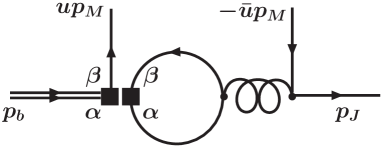
Figure 3: A typical charming penguin contribution, with charm quarks in the loop, and $\alpha$, $\beta$ are the color indices. The outgoing momenta $p$ and $p_{M}$ are $n$ and $\bar{n}$-collinear, respectively. Usoft interactions are not shown.

A typical charming penguin contribution is shown in Fig. 3. When the momentum transfer through the gluon is close to $4m_{c}^{2}$, the intermediate charm quark pair is almost on-shell and should be treated nonperturbatively, governed by usoft interactions. The long-distance contribution can be power counted as leading order in SCET Bauer:2005wb and cannot be disentangled from the bound state of the bottom quark. We can write the momentum of the charm quark pair as $2m_{c}v_{\bar{c}c}^{\mu}+k^{\mu}$, where $v_{\bar{c}c}^{\mu}$ is the velocity of the charm quark pair, and $k^{\mu}$ is the residual momentum of order $\Lambda_{\mathrm{QCD}}$. Note that $v_{\bar{c}c}^{\mu}$ is not the usual small velocity parameter $v^{*}$ in NRQCD. In the rest frame of the $B$ meson, we can write

$$2m_{c}v_{\bar{c}c}^{\mu}\sim\overline{n}\cdot p\frac{n^{\mu}}{2}+\bar{u}n\cdot p_{M}\frac{\overline{n}^{\mu}}{2},$$ (43)

where $v_{\bar{c}c}^{2}=1$. The momentum fraction of $\bar{u}$ of the antiquark in meson $M$ is given as

$$4r^{2}=\bar{u}x_{M},\qquad r\equiv m_{c}/m_{b},$$ (44)

where $\bar{u}=1-u$ and $x_{M}$ is close to 1 near the endpoint.

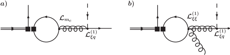
Figure 4: a) Nonperturbative penguins where charm quarks in the loop are treated as hard-collinear, with an insertion of $\mathcal{L}_{m_{c}}$ of order $\lambda^{0}$ in $\rm{SCET_{I}}$. b) one of the nonperturbative penguin contributions for massless quarks with the insertion of $\mathcal{L}_{\xi q}^{(1)}$ and $\mathcal{L}_{\xi\xi}^{(1)}$, each of which is suppressed by $\lambda$ in $\rm{SCET_{I}}$. Dashed line is an usoft quark, leading to additional endpoint suppression in forming a meson $M$.

There are two possible scenarios when we take appropriate limits of the charm quark mass compared to $m_{b}$. First, we can take the heavy quark limit $m_{b}\to\infty$ with $m_{c}\sim\sqrt{m_{b}\Lambda}$. In this case, $r^{2}$ is of order $\Lambda/m_{b}$ and the momentum of the charm pair, or the charm quark itself, becomes hard-collinear in the $n$ direction because $\bar{u}=4r^{2}/x_{M}$ is of order $\Lambda/m_{b}$. Therefore the outgoing antiquark with the momentum $\bar{u}p_{M}$ is an usoft quark, and the exchanged gluon has offshellness of order $\sqrt{m_{b}\Lambda}$. The long-distance charming penguin contribution, shown in Fig. 4 a), can be treated in the same way as that of the quarks with small mass, shown in Fig. 4 b). Since the usoft-collinear interaction is suppressed at least by $\lambda\sim\sqrt{\Lambda/m_{b}}$, the leading long-distance contribution is suppressed by $m_{c}/m_{b}$ at the operator level. In addition, the unbalanced endpoint configuration for the meson $M$ gives the endpoint suppression of order $\Lambda/m_{b}$. Therefore, the long-distance contribution in this limit is suppressed by $m_{c}\Lambda/m_{b}^{2}$. This power counting is in agreement with the expectation that the contribution of the charming penguin in this limit gives the same contribution as massless quarks, which is suppressed by $\Lambda^{2}/m_{b}^{2}$ Feldmann:2004mg . The reason why it is not of order $m_{q}\Lambda/m_{b}^{2}$ is because the quark mass insertion is replaced by the insertion of $\mathcal{L}_{\xi\xi}^{(1)}$.

The second scenario is to take the heavy quark limit $m_{b},~{}m_{c}\to\infty$ with fixed $r$, which is motivated by the fact that $\overline{u}=4r^{2}/x_{M}$ is near the central point experimentally. In this case, the power counting is different. The charm quark is regarded as a heavy quark and there is no endpoint suppression. The exchanged gluon in Fig. 3 has large offshellness $4m_{c}^{2}\sim m_{b}^{2}$, and is integrated out to obtain an operator of the form $[\bar{c}c]_{\mathrm{NR}}[\bar{\xi}_{\overline{n}}\xi_{n}]$. Here we suppress the Dirac structure and color indices, and the charm quark is treated as a heavy quark described by NRQCD. The nonperturbative charming penguin contribution is then obtained from the time-ordered product of this operator with the four-quark operators in the weak Hamiltonian of the form $[\bar{\xi}_{n}b_{v}][\bar{c}{c}]_{\mathrm{NR}}$. This leads to a contribution $\sim\alpha_{s}(2m_{c})v^{*}\mathcal{F}_{c\overline{c}}$ in agreement with Refs. Bauer:2005wb ; Bauer:2004tj , where the nonperturbative function $\mathcal{F}_{c\overline{c}}$ is comparable in size to the leading-order shape function $f$. Furthermore there is no endpoint suppression because the outgoing antiquark forming the meson $M$ is collinear with momentum fraction $\bar{u}=4r^{2}/x_{M}$, corresponding numerically to the the central region in the LCDA of the meson $M$.

We think that the second scenario is more plausible based on the actual value of $m_{c}/m_{b}$. As this is the more conservative of the two, we consider the nonperturbative charming penguins in the second scenario, which give larger contributions than the first scenario. As explained above, in the heavy quark limit $m_{b,c}\to\infty$ with $r$ fixed, the charming penguin can be of leading order, which can be expanded in powers of $\Lambda/m_{b,c}$ and $\alpha_{s}(2m_{c})$ in a consistent way. In this scheme, at leading order in $1/m_{b,c}$, the contribution is factorized into the $\overline{n}$-collinear part, the jet function, and a nonperturbative function. The derivation of the factorized form is presented in detail in Appendix B. At leading order in $\Lambda/m_{b,c}$, and to first order in $\alpha_{s}(2m_{c})$, the contribution of the charming penguin to the differential decay rate can be written as [see Eq. (107)]

$$\frac{d\Gamma_{\bar{c}c}(B\to X_{q}M)}{dE_{M}}=\frac{G_{F}^{2}}{8\pi}f_{M}^{2}m_{b}^{2}x_{M}^{3}\lambda_{c}^{(q)}\alpha_{s}(2m_{c})c_{q}^{BM}\phi_{M}\Bigr{(}u=1-\frac{4r^{2}}{x_{M}}\Bigr{)}\cdot 2\mathrm{Re}\mathcal{T}_{M}^{(q)*}{\cal F}_{c\overline{c}},$$ (45)

where $c_{q}^{BM}$ is defined in Appendix B and $\mathcal{T}_{M}^{(q)}$ is the hard kernel given in Table 1. Here $M=P,V_{L}$, while the contribution of $V_{T}$ is $1/m_{b,c}$ suppressed because of the spin flip. The function $\mathcal{F}_{c\overline{c}}$ does not depend on the outgoing meson $M$ or the jet $X$ because $\mathcal{F}_{c\overline{c}}$ is given by the nonperturbative effects arising only from the usoft interactions of the on-shell charm quark pair in the $B$ meson. Hence, up to the $B$ meson flavor, $\mathcal{F}_{c\overline{c}}$ is universal in all the decay modes where charm penguins contribute, and its size is experimentally measurable from various decay modes. In the isospin limit the $\mathcal{F}_{c\overline{c}}$ functions in $\overline{B}^{0}$ and $B^{-}$ decays are the same, and are equal to $\mathcal{F}_{c\overline{c}}$ in $B_{s}$ decays in the $SU(3)$ limit. Due to its nonperturbative nature it can, however, have a nonzero strong phase Bauer:2004tj .

In summary, the differential decay rate for the semi-inclusive decays at leading order in $1/m_{b}$, including the nonperturbative charming penguin at LO in $1/m_{c}$ and $\alpha_{s}(2m_{c})$, is

$$\frac{d\Gamma}{dE_{M}}(B\to X_{q}M) = \frac{G_{F}^{2}}{8\pi}f_{M}^{2}m_{b}^{2}x_{M}^{3}\Biggl{[}H_{M}^{(q)}(m_{b},\mu_{0})\mathcal{S}(x_{M},\mu_{0})$$

$$+\alpha_{s}(2m_{c})\lambda_{c}^{(q)}c_{q}^{BM}\phi_{M}\left(1-\frac{4r^{2}}{x_{M}}\right)2\mathrm{Re}\mathcal{T}_{M}^{(q)*}\mathcal{F}_{c\overline{c}}\Biggr{]}.$$

Phenomenological implications of this expression will be discussed in section VII.

VI Estimates of subleading corrections

To predict the branching ratios for $B\to XM$ more accurately, Eq. (V) can be systematically extended to higher orders in $1/m_{b}$ and $\alpha_{s}$. In this way one could also unambiguously determine whether a possible future discrepancy between experiment and predictions based on Eq. (42) is due to nonperturbative charming penguins or higher-order corrections. A full analysis of the higher-order corrections is beyond the scope of this paper, but we identify typical subleading corrections and estimate their size. The subleading corrections, suppressed by powers of $\Lambda/m_{b}$, are of two types: (i) corrections to the heavy-to-light current leading to the subleading $B$-meson shape functions, some of which are already well known from the analyses of $\overline{B}\to X_{s}\gamma$ and $\overline{B}\to X_{u}l\bar{\nu}$ inclusive decays Bauer:2001mh ; Leibovich:2002ys ; Bauer:2002yu ; Lee:2004ja ; Bosch:2004cb , and (ii) corrections to the $\overline{n}$-collinear currents forming the light meson $M$, which appear as the twist-3 LCDA and the $SU(3)$ breaking effects in the twist-2 LCDA.

Let us consider the corrections of the first type. The convolution $\mathcal{S}$ of the jet function and the $B$ meson shape function in Eq. (IV) can be expanded to higher orders in $1/m_{b}$ as

$$\mathcal{S}(x_{M})=\mathcal{S}^{(0)}(x_{M})+\Bigl{(}\mathcal{S}^{(1)}_{hl}(x_{M})+\mathcal{S}^{(1)}_{\overline{n}}(x_{M})\Bigr{)}+\cdots,$$ (47)

where $\mathcal{S}_{hl}^{(1)}$ is the subleading corrections to the heavy-to-light current and $\mathcal{S}_{\overline{n}}^{(1)}$ is the usoft corrections to the $\overline{n}$-collinear current. Using the results of Ref. Bosch:2004cb , the sum $\mathcal{S}^{(0)}+\mathcal{S}_{hl}^{(1)}$ can be related to the imaginary part of the time-ordered product, $W_{\mu\nu}$,

$$\frac{1}{m_{b}}\Bigl{(}\mathcal{S}^{(0)}+\mathcal{S}_{hl}^{(1)}\Bigr{)}=W_{\mu\nu}\frac{\overline{n}^{\mu}\overline{n}^{\nu}}{4},$$ (48)

where the factor $\overline{n}^{\mu}/2$ comes from the $\overline{n}$-collinear current $\langle\bar{\xi}_{\overline{n}}\gamma^{\mu}\xi_{\overline{n}}\rangle=\overline{n}^{\mu}\langle\bar{\xi}_{\overline{n}}{n}\!\!\!/\xi_{\overline{n}}\rangle/2$. Taking the ratio with respect to $\overline{B}\to X_{s}\gamma$ gives the difference

$$\mathcal{S}_{hl}^{(1)}-\mathcal{S}_{\gamma}^{(1)} = \Bigl{(}\mathcal{S}^{(0)}+\mathcal{S}_{hl}^{(1)}\Bigr{)}-\Bigl{(}\mathcal{S}^{(0)}+\mathcal{S}_{\gamma}^{(1)}\Bigr{)}$$

$$\sim 2\int dn\cdot l~{}v(n\cdot l)~{}\delta(m_{b}(1-x)+n\cdot l)=-\frac{2}{m_{b}^{2}}H_{2}(1-x),$$

where $x=x_{M}=x_{\gamma}$ is chosen. The subleading shape functions $v$ and $H_{2}$ are defined in Refs. Bosch:2004cb and Bauer:2001mh , respectively. In particular, $H_{2}$ is proportional to $\lambda_{2}=\langle\bar{B}_{v}|\bar{b}_{v}g_{s}\sigma_{\mu\nu}G^{\mu\nu}b_{v}|\bar{B}_{v}\rangle/12\sim 0.12\ \mathrm{GeV}^{2}.$ Taking a broad cut $E_{M}\geq 2.0$ GeV, this contribution should not exceed $10\%$ compared to the leading contribution, unless there is an enhancement in the coefficient.

The subleading correction $\mathcal{S}_{\overline{n}}^{(1)}$ comes from the usoft interactions with the $\overline{n}$-collinear currents, which lead to new subleading $B$ meson shape functions. The subleading operators obtained by inserting the usoft gauge-invariant term $Y_{\overline{n}}^{\dagger}i{D}\!\!\!\!/^{\perp}_{us}Y_{\overline{n}}$ are suppressed by $\lambda^{2}$ in $\rm{SCET_{I}}$, but they should be included in $\rm{SCET_{II}}$ because they are suppressed by $\Lambda/m_{b}$. The nonzero contributions come only from the color-octet four-quark operators

$$\begin{split}{\cal O}_{iA}^{(1)}(u)&=2\big{(}\bar{q}_{n}Y_{n}^{\dagger}Y_{\overline{n}}\gamma^{\mu}P_{L}T^{a}Y_{\overline{n}}^{\dagger}b_{v}\big{)}\cdot\Big{[}\bar{q^{\prime}}_{\overline{n}}\,\gamma_{\mu}\,P_{L,R}\,T^{a}\,Y_{\overline{n}}^{\dagger}i{D}\!\!\!\!/^{\perp}_{us}Y_{\overline{n}}\,\frac{1}{n\cdot{\cal P}}\,{n}\!\!\!/\,q^{\prime\prime}_{\overline{n}}\Big{]}_{u},\\ {\cal O}_{iB}^{(1)}(u)&=2\big{(}\bar{q}_{n}Y_{n}^{\dagger}Y_{\overline{n}}\gamma^{\mu}P_{L}T^{a}Y_{\overline{n}}^{\dagger}b_{v}\big{)}\cdot\Big{[}\bar{q^{\prime}}_{\overline{n}}\;{n}\!\!\!/\frac{1}{n\cdot{\cal P}^{\dagger}}Y_{\overline{n}}^{\dagger}i\overleftarrow{{D}\!\!\!\!/}^{\perp}_{us}Y_{\overline{n}}\,T^{a}\gamma_{\mu}\,P_{L,R}\,q^{\prime\prime}_{\overline{n}}\Big{]}_{u},\end{split}$$ (50)

where the flavor and chirality structure is the same as the corresponding leading operators ${\cal O}_{i}$ in Eq. (8). Because of reparameterization invariance Chay:2002vy ; Manohar:2002fd , the Wilson coefficients of ${\cal O}_{i,A}^{(1)}(u)+{\cal O}_{i,B}^{(1)}(u)$ are the same as those for the leading color-octet operators in Eq. (12), which are presented in Appendix A.

After some calculation, the matrix elements of these operators which do not vanish trivially from the flavor content are nonzero only for specific values of $i$ due to the helicity structure. They are given by

$$\langle{\cal O}_{i,A}^{(1)}(u)\rangle = \frac{if_{M}}{N}\frac{\phi_{M}(u)}{\overline{u}}\langle X_{q}|\overline{q}_{n}\Bigl{[}Y_{n}^{\dagger}i{D}\!\!\!\!/^{\perp}_{us}Y_{\overline{n}}\Bigr{]}P_{L}Y_{\overline{n}}^{\dagger}b_{v}|B\rangle,\ (i=1,2,4,5),$$ (51)

$$\langle{\cal O}_{i,B}^{(1)}(u)\rangle = (\delta_{VM}-\delta_{PM})\frac{if_{M}}{N}\frac{\phi_{M}(u)}{u}\langle X_{q}|\overline{q}_{n}Y_{n}^{\dagger}Y_{\overline{n}}\Bigl{[}Y_{\overline{n}}^{\dagger}i\overleftarrow{{D}\!\!\!\!/}^{\perp}_{us}\Bigr{]}P_{L}b_{v}|B\rangle,\ (i=3,6),$$

where $\delta_{PM}$, $\delta_{VM}$ are Kronecker deltas, and we use Eqs. (97) and (98) in Appendix B for the matrix elements of the collinear current. For the matrix elements of the heavy-to-light current, we need the time-ordered products with $J_{H}^{\dagger}$,

$$T_{A}^{(2)} = \frac{2i}{m_{b}m_{B}}\int d^{4}z~{}e^{-ip_{M}\cdot z}\langle B|\mathrm{T}J_{H}^{\dagger}(z)~{}\overline{q}_{n}\Bigl{[}Y_{n}^{\dagger}i{D}\!\!\!\!/^{\perp}_{us}Y_{\overline{n}}\Bigr{]}P_{L}Y_{\overline{n}}^{\dagger}b_{v}(0)|B\rangle,$$ (52)

$$T_{B}^{(2)} = \frac{2i}{m_{b}m_{B}}\int d^{4}z~{}e^{-ip_{M}\cdot z}\langle B|\mathrm{T}J_{H}^{\dagger}(z)~{}\overline{q}_{n}Y_{n}^{\dagger}Y_{\overline{n}}\Bigl{[}Y_{\overline{n}}^{\dagger}i\overleftarrow{{D}\!\!\!\!/}^{\perp}_{us}\Bigr{]}P_{L}b_{v}(0)|B\rangle.$$

They can be factorized into the jet function and subleading $B$-meson shape functions,

$$T_{A,B}^{(2)}=-2\int^{\overline{\Lambda}}_{-m_{b}(1-x_{M})}dn\cdot l~{}f^{(1)}_{A,B}(n\cdot l)~{}J_{P}\Bigl{(}m_{b}(1-x_{M})+n\cdot l+i\epsilon\Bigr{)},$$ (53)

where the subleading shape functions are defined as

$$f_{A}^{(1)}(n\cdot l) = \frac{1}{m_{b}}\langle B_{v}|\bar{b}_{v}Y_{n}\delta(n\cdot l-n\cdot i\partial)\frac{{\overline{n}}\!\!\!/{n}\!\!\!/}{4}\Bigl{[}Y_{n}^{\dagger}i{D}\!\!\!\!/^{\perp}_{us}Y_{\overline{n}}\Bigr{]}Y_{\overline{n}}^{\dagger}b_{v}|B_{v}\rangle,$$ (54)

$$f_{B}^{(1)}(n\cdot l) = \frac{1}{m_{b}}\langle B_{v}|\bar{b}_{v}Y_{n}\delta(n\cdot l-n\cdot i\partial)\frac{{\overline{n}}\!\!\!/{n}\!\!\!/}{4}Y_{n}^{\dagger}Y_{\overline{n}}\Bigl{[}Y_{\overline{n}}^{\dagger}i\overleftarrow{{D}\!\!\!\!/}^{\perp}_{us}\Bigr{]}b_{v}(0)|B_{v}\rangle.$$

The shape functions $f_{A,B}^{(1)}$ are different from the subleading shape functions appearing in $\overline{B}\to X_{s}\gamma$ and $\overline{B}\to X_{u}l\bar{\nu}$, due to the presence of $Y_{\overline{n}}^{(\dagger)}$, which cannot be neglected at subleading order. At present we cannot estimate their size, but there is no reason to expect a dramatic enhancement from the insertion of $Y_{\overline{n}}^{(\dagger)}$. However, these contributions can be numerically significant in the decays that are very small at LO in $1/m_{b}$. These are the color-suppressed $\Delta S=0$ tree decays $\overline{B}_{s}^{0}\to\{\pi^{0},\rho^{0},\omega\}X_{\bar{s}}^{0}$, the QCD penguin-dominated $\Delta S=0$ and $\Delta S=1$ decays $\overline{B}^{0}\to\phi X^{0},B^{-}\to\phi X^{-}$ and $\overline{B}_{s}^{0}\to\omega X_{s\bar{s}}^{0}$ and the $\lambda_{u}^{(s)}$ part of the amplitudes in $\overline{B}_{s}^{0}\to\{\pi^{0},\rho^{0}\}X_{s\bar{s}}^{0}$. For these decays, the Wilson coefficients of the LO operators convoluted with the asymptotic LCDA ($|\phi\otimes\mathcal{C}_{2}^{u}|\sim 0.08$ and $|\phi\otimes(\mathcal{C}_{5}+\mathcal{C}_{6})|\sim 0.005$) are much smaller than those for the color-octet operators ($|\phi\otimes\mathcal{C}_{2}^{u}|\sim 1.9$ and $|\phi\otimes(\bar{\mathcal{C}}_{5}+\bar{\mathcal{C}}_{6})|\sim 0.15$). The subleading contributions can thus be numerically large in spite of the $1/2N$ suppression. Note that this is not a sign of failure of the $1/m_{b}$ expansion, but due to the hierarchy of the Wilson coefficients.

There is another contribution shown in Fig. 5, from the time-ordered products of the $\overline{n}$-collinear currents and $\mathcal{L}_{\xi\xi}^{(1)}$,

$$\mathcal{L}_{\xi\xi}^{(1)}=\bar{\xi}_{\overline{n}}W_{\overline{n}}\Bigl{(}Y_{\overline{n}}^{\dagger}i{D}\!\!\!\!/_{us}^{\perp}Y_{\overline{n}}\Bigr{)}\frac{1}{n\cdot\mathcal{P}}W_{\overline{n}}^{\dagger}i{D}\!\!\!\!/_{\overline{n}}^{\perp}\frac{{\overline{n}}\!\!\!/}{2}\xi_{\overline{n}}+\bar{\xi}_{\overline{n}}i{D}\!\!\!\!/_{\overline{n}}^{\perp}\frac{{\overline{n}}\!\!\!/}{2}W_{\overline{n}}\frac{1}{n\cdot\mathcal{P}}\Bigl{(}Y_{\overline{n}}^{\dagger}i{D}\!\!\!\!/_{us}^{\perp}Y_{\overline{n}}\Bigr{)}\frac{{\overline{n}}\!\!\!/}{2}W_{\overline{n}}^{\dagger}\xi_{\overline{n}}.$$ (55)

The intermediate legs in Fig. 5 are hard-collinear and give a jet function of the form $1/\overline{n}\cdot k$. The relevant LCDA for $M$ are suppressed by $\Lambda/m_{b}$ due to the presence of $iD_{\overline{n}}^{\perp}$. But it is not known whether this process factorizes, and we leave a full analysis for future work.

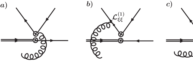
Figure 5: Subleading usoft interactions induced from the $\overline{n}$-collinear currents. In Diagrams b) and c), the dots denote the $\lambda$-suppressed interaction in $\mathcal{L}_{\xi\xi}^{(1)}$.

We now consider the contributions from the $(S-P)\times(S+P)$ four-quark operator. At leading order it matches onto $\overline{q^{\prime}}_{n}(1-\gamma_{5})b\cdot\overline{q}_{\overline{n}}(1+\gamma_{5})q_{\overline{n}}^{\prime}$, which vanishes because of spin symmetry. At subleading order it matches onto

$$\begin{split}{\cal O}^{(1)}_{S+P}=-2\sum_{q^{\prime}=u,d,s}&\big{(}\overline{q^{\prime}}_{n}\,{\overline{n}}\!\!\!/\,P_{R}Y_{n}^{\dagger}b_{v}\big{)}\Big{(}\overline{q}_{\overline{n}}\,P_{R}\frac{1}{n\cdot\mathcal{P}}W_{\overline{n}}^{\dagger}i{D}\!\!\!\!/_{\overline{n}}^{\perp}W_{\overline{n}}\,{n}\!\!\!/\,{q^{\prime}}_{\bar{n}}\Big{)}+\\ +&\big{(}\overline{q^{\prime}}_{n}\,{\overline{n}}\!\!\!/\,P_{R}Y_{n}^{\dagger}b_{v}\big{)}\Big{(}\overline{q}_{\overline{n}}\,{n}\!\!\!/\,\,W_{\overline{n}}^{\dagger}i\overleftarrow{{D}\!\!\!\!/}_{\overline{n}}^{\perp}W_{\overline{n}}\frac{1}{n\cdot\mathcal{P}^{\dagger}}P_{R}{q^{\prime}}_{\bar{n}}\Big{)},\end{split}$$ (56)

where for the heavy-to-light current we have used the relation ($2v^{\mu}=n^{\mu}+\overline{n}^{\mu}$)

$$2\overline{q}^{\prime}_{n}P_{L}Y_{n}^{\dagger}b_{v}=2\overline{q}^{\prime}_{n}P_{L}{v}\!\!\!/Y_{n}^{\dagger}b_{v}=\overline{q}^{\prime}_{n}{\overline{n}}\!\!\!/P_{R}Y_{n}^{\dagger}b_{v}.$$ (57)

In semi-inclusive $B$ decays, the amplitude from this operator factorizes using the twist-3 LCDA Hardmeier:2003ig . At order $1/m_{b}$ it contributes through the time-ordered product with the leading heavy-to-light current as

$$T_{S+P}=\frac{i}{m_{B}}\int d^{4}z~{}e^{-ip_{M}\cdot z}\langle B|\mathrm{T}J_{H}^{\dagger}(z)~{}\overline{q}_{n}^{\prime}{\overline{n}}\!\!\!/P_{R}Y_{\overline{n}}^{\dagger}b_{v}(0)|B\rangle.$$ (58)

This vanishes because

$$\langle B|\mathrm{T}J_{H}^{\dagger}(z)~{}\overline{q}_{n}{\overline{n}}\!\!\!/P_{R}Y_{\overline{n}}^{\dagger}b_{v}(0)|B\rangle\propto\langle B|\overline{b}_{v}Y_{n}(\tfrac{\overline{n}\cdot z}{2}){\overline{n}}\!\!\!/P_{L}\,{n}\!\!\!/\,{\overline{n}}\!\!\!/P_{R}Y_{\overline{n}}^{\dagger}b_{v}(0)|B\rangle=0.$$ (59)

Therefore the nonzero contribution comes from the time-ordered products of $\mathcal{O}_{S+P}^{(1)}$ with the subleading operators of $J_{H}^{\dagger}$, suppressed by $m_{q}/m_{b}$ Chay:2005ck , or from the time-ordered products of $\mathcal{O}_{S+P}^{(1)}$ with itself. Both are of order $1/m_{b}^{2}$, but the latter may not be numerically negligible. In the QCD factorization approach Beneke:1999br , the contributions corresponding to ${\cal O}^{(1)}_{S+P}$ lead to formally suppressed but numerically large “chirally enhanced” contributions. In SCET ${\cal O}^{(1)}_{S+P}$ is also formally suppressed, while its matrix elements remain unknown and could be numerically large. Because of this uncertainty, the decay rates and the CP asymmetries presented in the next section for modes with small tree-level amplitudes should be regarded only as a rough estimate.

Finally, we discuss the $SU(3)$ breaking corrections to Eq. (42). The $SU(3)$ breaking due to different light-quark flavors in the inclusive jet is suppressed by $m_{s}^{2}/m_{b}\Lambda$ Chay:2005ck and thus negligible, but the $SU(3)$ corrections due to the strangeness content of meson $M$ are not negligible. These are realized in SCET by inserting the strange quark mass term Leibovich:2003jd ; Rothstein:2003wh

$$\mathcal{L}_{m}=m_{s}~{}\overline{\xi}_{\bar{n}}\Biggl{[}i{D}\!\!\!\!/_{\overline{n}}^{\perp},\frac{1}{n\cdot iD_{\overline{n}}}\Biggr{]}\frac{{n}\!\!\!/}{2}\xi_{\bar{n}}$$ (60)

in the leading $\overline{n}$-collinear currents with the final-state $s$ quark in Fig. 6. It can be written as

$$A_{s}(u)=\frac{-i}{f_{M}E_{M}}\langle M|~{}\mathrm{T}~{}\big{[}\overline{s}_{\bar{n}}{n}\!\!\!/P_{L}q_{\bar{n}}(0)\big{]}_{u}\cdot i\int d^{4}z\mathcal{L}_{m}(z)~{}|0\rangle.$$ (61)

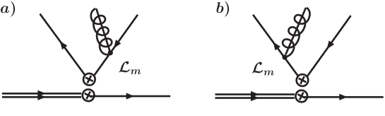
Figure 6: The insertion of the strange quark mass in the $\overline{n}$-collinear currents in $\rm{SCET_{II}}$. Diagrams a) and b) represent the possible strange quark mass insertions for the strange quark in Eq. (61) where the external particle is a strange quark.

For the final-state $\overline{s}$ quark, a hermitian conjugate of Eq. (61), $A_{\bar{s}}(u)$, is needed with $A_{\bar{s}}(u)=A_{s}(\bar{u})$. If $m_{s}$ is comparable to $iD_{\overline{n}}^{\perp}\sim\Lambda$, $\mathcal{L}_{m}$ is of leading order in $\rm{SCET_{II}}$, suppressed only by $m_{s}/\Lambda$.

The $SU(3)$ breaking affects meson decay constants and the LCDAs. One finds to leading order in $SU(3)$-breaking $\phi_{\bar{K}}(u)=\phi(u)+A_{s}(u)$, $\phi_{K}(u)=\phi(u)+A_{s}(\bar{u})$ and $\phi_{\eta}(u)=\phi(u)+2\big{(}A_{s}(u)+A_{s}(\bar{u})\big{)}/3$ for the LCDA of $K^{-}(\overline{K}^{0}),K^{+}(K^{0})$ and $\eta$, where $\phi(u)$ is the pion LCDA. Since $\int_{0}^{1}\phi_{M}(u)du=1=\int_{0}^{1}\phi(u)du$ one has a constraint

$$\int_{0}^{1}A_{s}(u)du=0.$$ (62)

It is also straightforward to check that these LCDA satisfy the relation Chen:2003fp $\phi_{\pi}(u,\mu)+3\phi_{\eta}(u,\mu)=2\Bigl{[}\phi_{K^{+}}(u,\mu)+\phi_{K^{-}}(u,\mu)\Bigl{]}=2\Bigl{[}\phi_{K^{0}}(u,\mu)+\phi_{\bar{K}^{0}}(u,\mu)\Bigl{]}.$ From power counting one expects the relative size of the $SU(3)$ breaking contribution to be of order $m_{s}/\Lambda\sim 20$%. Recent QCD sum rules predictions can be found in Refs. Khodjamirian:2003xk ; Ball:2006wn ; Ball:2004rg ; Ball:2004ye .

VII Phenomenology

In this section we collect the predictions for $B\to XM$ decay rates and direct CP asymmetries, defined as

$$A_{CP}=\frac{{d\Gamma(\overline{B}\to XM)}/{dE_{M}}-d\Gamma(B\to XM)/dE_{M}}{d\Gamma(\overline{B}\to XM)/dE_{M}+d\Gamma(B\to XM)/dE_{M}},$$ (63)

while treating the charming penguins as perturbative. Once the experimental data become available, one of the modes can be used to determine the nonperturbative charm contribution $\mathcal{F}_{c\overline{c}}$ and then modify the predictions according to Eq. (V). To reduce the hadronic uncertainty, we normalize the branching ratios of $\overline{B}^{0}\to XM$, $B^{-}\to XM$, and $\overline{B}_{s}^{0}\to XM$ to the decay rates $\overline{B}^{0}\to X_{s}^{0}\gamma$, $B^{-}\to X_{s}^{-}\gamma$, and $\overline{B}_{s}^{0}\to X_{s\bar{s}}^{0}\gamma$ in the endpoint region, respectively [See Eq. (42).] The only remaining nonperturbative input is then the light meson LCDAs. Expanding in terms of the Gegenbauer polynomials,

$$\phi_{M}(u,\mu)=6u\bar{u}\big{[}1+\sum_{n=1}^{\infty}a_{n}^{M}(\mu)C_{n}^{3/2}(2u-1)\big{]},$$ (64)

we truncate the series at $n=2$ and use isospin symmetry to set $a_{1}^{M}=0$ for mesons not containing a strange quark. We fix the remaining coefficients using the results from QCD sum rules, while conservatively doubling the errors quoted in the literature. This gives at $\mu=2$ GeV: $a_{1}^{K}=0.05\pm 0.05$, $a_{2}^{K}=0.23\pm 0.23$ Ball:2006wn , $a_{1}^{K^{*}}=0.08\pm 0.13$, Ball:2004rg , $a_{2}^{\pi}=0.09\pm 0.15$ Ball:2004ye , $a_{2}^{K^{*}}=0.07\pm 0.08$, $a_{2}^{\rho}=0.14\pm 0.15$, $a_{2}^{\phi}=0.\pm 0.15$ Ball:2004rg , while for the $\omega$ LCDA $a_{2}^{\omega}=0.\pm 0.2$ is used for lack of better information.

Mode	Br(Mode)/Br($B\to X_{s}\gamma$)	Exp. (2-body)	$A_{CP}$
$\overline{B}^{0}\to K^{-}X^{+}$	$0.16\pm 0.09\pm 0.05$	$>0.078$	$0.30\pm 0.16\pm 0.01$
$\overline{B}^{0}\to K^{*-}X^{+}$	$0.28\pm 0.16\pm 0.07$	$>0.026$	$0.31\pm 0.16\pm 0.02$
$\overline{B}^{0}\to\phi X_{s}^{0}$	$0.22\pm 0.13\pm 0.03$	$>0.034$	$0.0089\pm 0.0050\pm 0.0016$
$B^{-}\to\overline{K}^{0}X^{-}$	$0.20\pm 0.11\pm 0.06$	$>0.067$	$0.0097\pm 0.0048\pm 0.0006$
$B^{-}\to\overline{K}^{*0}X^{-}$	$0.34\pm 0.19\pm 0.08$	$>0.040$	$0.0084\pm 0.0046\pm 0.0019$
$B^{-}\to\phi X_{s}^{-}$	$0.22\pm 0.13\pm 0.03$	$>0.035$	$0.0089\pm 0.0050\pm 0.0016$
$\overline{B}_{s}^{0}\to\pi^{0}X_{s\bar{s}}^{0}$	$(1.0\pm 0.6\pm 0.2)\times 10^{-2}$	$-$	$-$
$\overline{B}_{s}^{0}\to K^{-}X_{\bar{s}}^{+}$	$0.16\pm 0.09\pm 0.05$	$-$	$0.30\pm 0.16\pm 0.01$
$\overline{B}_{s}^{0}\to\rho^{0}X_{s\bar{s}}^{0}$	$(2.4\pm 1.4\pm 0.5)\times 10^{-2}$	$-$	$-$
$\overline{B}_{s}^{0}\to\omega X_{s\bar{s}}^{0}$	$(2.8\pm 3.4\pm 0.7)\times 10^{-3}$	$-$	$-$
$\overline{B}_{s}^{0}\to K^{*-}X_{\bar{s}}^{+}$	$0.28\pm 0.16\pm 0.07$	$-$	$0.32\pm 0.16\pm 0.02$

Table 2: Predictions for decay rates and direct CP asymmetries for $\Delta S=1$ semi-inclusive hadronic decays are given in the second and fourth column, respectively. The first errors are an estimate of the $1/m_{b}$ corrections, while the second errors are due to errors on the Gegenbauer coefficients in the expansion of the LCDA. The third column gives lower bounds on inclusive decay rates obtained by summing over measured two-body decays and normalizing to $b\to s\gamma$ decay with $E_{\rm min}=2.0$ GeV ($90\%$ CL lower bounds are used).

Direct CP asymmetries in Eq. (63) are nonzero only in the presence of nonzero strong phases. These are generated by integrating out on-shell light quarks in a loop when matching full QCD to $\rm{SCET_{I}}$ at NLO in $\alpha_{s}$. We therefore use the NLO matching expressions for the Wilson coefficients $\mathcal{C}_{i}^{p}$ at $\mu=m_{b}$ even though the evolution to the hard-collinear scale $\mu_{0}\sim\sqrt{\Lambda m_{b}}$ is performed at NLL. Note that this running cancels to a large extent in the ratios of decay rates (only the running of $a_{n}^{M}(\mu),n\geq 1$ remains), giving in effect the Wilson coefficients with NLO accuracy at the hard-collinear scale $\mu_{0}$.

For definitiveness, we choose $\mu_{0}=2$ GeV for the hard-collinear scale, which corresponds to the experimental cut $p_{X}^{2}<(2{\rm\ GeV})^{2}$ on the inclusive jet invariant mass. The corresponding predictions are listed in Tables 2 and 3 for $\Delta S=1$ and $\Delta S=0$ decays respectively. The predicted partial decay widths $d\Gamma(B\rightarrow XM)/dE_{M}$ in principle depend on the light meson energy $E_{M}$. In the endpoint region the dependence on $x_{M}=2E_{M}/m_{B}=1+{(m_{M}^{2}-p_{X}^{2})}/{m_{B}^{2}}$ is, however, a subleading effect, so we set $x_{M}=1$ in Tables 2 and 3.

Mode	Br(Mode)/Br($B\to X_{s}\gamma$)	Exp. (2-body)	$A_{CP}$
$\overline{B}^{0}\to\pi^{-}X^{+}$	$0.67\pm 0.37\pm 0.14$	$>0.038$	$-0.040\pm 0.021\pm 0.004$
$\overline{B}^{0}\to K^{0}X_{s}^{0}$	$(9.1\pm 5.3\pm 3.1)\times 10^{-3}$	$>2.0\times 10^{-3}$	$-0.15\pm 0.11\pm 0.01$
$\overline{B}^{0}\to\phi X^{0}$	$(2.0\pm 2.0\pm 0.1)\times 10^{-4}$	$-$	$-$
$\overline{B}^{0}\to\rho^{-}X^{+}$	$1.76\pm 0.97\pm 0.35$	$>0.10$	$-0.039\pm 0.021\pm 0.004$
$\overline{B}^{0}\to K^{*0}X_{s}^{0}$	$(1.4\pm 0.8\pm 0.5)\times 10^{-2}$	$-$	$-0.17\pm 0.11\pm 0.03$
$B^{-}\to K^{0}X_{s}^{-}$	$(9.1\pm 5.3\pm 3.1)\times 10^{-3}$	$>2.5\times 10^{-3}$	$-0.15\pm 0.11\pm 0.01$
$B^{-}\to\phi X^{-}$	$(2.0\pm 2.0\pm 0.1)\times 10^{-4}$	$-$	$-$
$B^{-}\to K^{*0}X_{s}^{-}$	$(1.4\pm 0.8\pm 0.5)\times 10^{-2}$	$-$	$-0.17\pm 0.11\pm 0.03$
$\overline{B}_{s}^{0}\to\pi^{0}X_{\bar{s}}^{0}$	$(4.1\pm 4.1\pm 2.6)\times 10^{-3}$	$-$	$-$
$\overline{B}_{s}^{0}\to\pi^{-}X_{\bar{s}}^{+}$	$0.67\pm 0.37\pm 0.14$	$-$	$-0.040\pm 0.021\pm 0.004$
$\overline{B}_{s}^{0}\to\rho^{0}X_{\bar{s}}^{0}$	$(1.3\pm 1.3\pm 0.7)\times 10^{-2}$	$-$	$-$
$\overline{B}_{s}^{0}\to\rho^{-}X_{\bar{s}}^{+}$	$1.76\pm 0.97\pm 0.35$	$-$	$-0.039\pm 0.021\pm 0.004$
$\overline{B}_{s}^{0}\to\omega X_{\bar{s}}^{0}$	$(1.1\pm 1.1\pm 0.9)\times 10^{-2}$	$-$	$-$

Table 3: Predictions for decay widths and direct CP asymmetries of $\Delta S=0$ semi-inclusive hadronic decays. The first errors are an estimate of the $1/m_{b}$ corrections, while the second errors are due to errors on the Gegenbauer coefficients in the expansion of the LCDAs. The third column gives lower bounds on inclusive decay rates obtained by summing over measured two-body decays and normalizing to $b\to s\gamma$ decay with $E_{\rm min}=2.0$ GeV ($90\%$ CL lower bounds are used).

The two errors quoted in Tables 2 and 3 are an estimate of subleading corrections and the errors due to coefficients of the Gegenbauer expansion of LCDAs. Since the predictions are made to NLO in $\alpha_{s}(m_{b})$ but only to LO in $1/m_{b}$, the largest corrections are expected to arise from the $1/m_{b}$ terms. These are estimated by independently varying the magnitudes of the leading terms proportional to $\lambda_{u,c,t}^{(s),(d)}$ by 20% $\sim O(\Lambda/m_{b})$ and the strong phase by $5^{\circ}$. This latter variation estimates the error on the strong phase arising from the uncalculated $\alpha_{s}(m_{b})/m_{b}$ or $\alpha_{s}^{2}(m_{b})$ terms. A $100\%$ error is assigned to predictions for branching ratios in color-suppressed tree and QCD penguin-dominated $\Delta S=0$ decays where the $1/m_{b}$ corrections are sizable compared to the leading results due to the hierarchy of Wilson coefficients. No prediction on CP asymmetries is given for these modes or for the affected QCD penguin-dominated $\Delta S=1$ decays.

To understand better the relative sizes of different branching ratios, it is useful to split the amplitudes for the semi-inclusive decays according to the CKM elements. Using the unitarity of the CKM matrix $\lambda_{t}^{(q)}=-\lambda_{u}^{(q)}-\lambda_{c}^{(q)}$, the amplitude can be rewritten in terms of the “tree” amplitude $T_{B\to MX}$ and the “penguin” amplitude $P_{B\to MX}$ as

$$A(B\to MX)=\lambda_{u}^{(q)}T_{B\to MX}+\lambda_{c}^{(q)}P_{B\to MX},$$ (65)

with $q=d,s$ for $\Delta S=0,1$ decays respectively. The “tree” amplitudes receive contributions from $O_{1,2}^{u}$ in Eq. (6), the “penguin” amplitudes from $O_{1,2}^{c}$ (charming penguins), while the QCD and electroweak penguin operators contribute to both amplitudes. The combinations of the CKM elements exhibit the following hierarchy

$$\lambda_{c}^{(s)}\sim\lambda_{C}^{2},\quad\lambda_{u,c}^{(d)}\sim\lambda_{C}^{3},\quad\lambda_{u}^{(s)}\sim\lambda_{C}^{4},$$ (66)

where $\lambda_{C}=0.23$ is the Cabibbo angle. In $\Delta S=0$ decays, the two CKM factors in Eq. (65) are of comparable size. In $\Delta S=1$ decays, on the other hand, there is a hierarchy between the two terms in Eq. (65) since $|\lambda_{u}^{(s)}/\lambda_{c}^{(s)}|\sim\lambda_{C}^{2}$. To first order in this small ratio, the quantity

$$A_{CP}^{\Delta S=1}(B\to MX)=-2\mathrm{Im}\left(\frac{\lambda_{u}^{(s)}}{\lambda_{c}^{(s)}}\right)\mathrm{Im}\left(\frac{T_{B\to MX}}{P_{B\to MX}}\right),$$ (67)

with $-2\mathrm{Im}(\lambda_{u}^{(s)}/\lambda_{c}^{(s)})=0.037$, which sets a typical size of the CP asymmetries. The size of the direct CP asymmetries also crucially depends on the ratio of “tree” over “penguin” amplitudes, as can be seen in Table 2. This can be estimated from the sizes of the Wilson coefficients at $\mu=m_{b}$ (convoluted with the asymptotic form of LCDA) that are given in Table 4. The modes that receive contributions from the operator ${\cal O}_{1}^{u}$, $\overline{B}_{s}^{0}\to K^{(*)-}X_{\bar{s}}^{+}$ and $\overline{B}^{0}\to K^{(*)-}X^{+}$, have $T_{B\to MX}>P_{B\to MX}$ and thus have larger CP asymmetries. The rest of the modes listed in Table 2 do not receive these large tree contributions and thus have smaller CP asymmetries.

	$~{}~{}\mathcal{C}_{1}^{u}~{}~{}$	$~{}~{}\mathcal{C}_{2}^{u}~{}~{}$	$~{}~{}\mathcal{C}_{1}^{c}~{}~{}$	$~{}~{}\mathcal{C}_{2}^{c}~{}$	$~{}~{}\mathcal{C}_{3}~{}~{}$	$~{}~{}\mathcal{C}_{4}^{u}~{}~{}$	$~{}~{}\mathcal{C}_{4}^{c}~{}~{}$	$~{}~{}\mathcal{C}_{5}~{}~{}$	$~{}~{}\mathcal{C}_{6}~{}~{}$
Abs	$0.89$	$0.080$	$0.0011$	$0.012$	$0.00037$	$0.029$	$0.032$	$0.010$	$0.0061$
Arg	${0.9^{\circ}}$	${-99^{\circ}}$	${79^{\circ}}$	${181^{\circ}}$	${7.5^{\circ}}$	${-150^{\circ}}$	${-163^{\circ}}$	$14^{\circ}$	$-151^{\circ}$

Table 4: The magnitudes and strong phases of the Wilson coefficients at $\mu=m_{b}$ (using the notation $\mathcal{C}_{3,5,6}=\mathcal{C}^{u}_{3,5,6}=\mathcal{C}^{c}_{3,5,6}$) convoluted with the asymptotic form of the LCDA $\phi=6u\bar{u}$.

Note that the direct CP asymmetries are nonzero only if the two interfering amplitudes in Eq. (65) have different strong phases. In the $\Delta S=0$ decays $\overline{B}^{0}\to\phi X^{0}$ and $B^{-}\to\phi X^{-}$, the two amplitudes $T_{B\to MX},P_{B\to MX}$ are the same at LO in $1/m_{b}$ and the CP asymmetries vanish. This may change at higher orders, but no prediction for $A_{CP}$ for these modes is given in Table 3.

For color-suppressed two-body decays, the leading order tree amplitude in $\rm{SCET_{I}}$ comes from $O_{2}$. However, when matching onto $\rm{SCET_{II}}$, the hard-spectator contribution from $O_{1}$ can compete with the leading order term. For semi-inclusive decays considered in this paper, in which the spectator quark does not enter the outgoing meson $M$, there are no hard-spectator interactions. Thus, due to the hierarchy of the Wilson coefficients (using values in Table 4)

$$\Big{|}\int_{0}^{1}du\;6u\bar{u}\,\mathcal{C}_{2}^{u}(u)\Big{|}\sim 0.10\;\Big{|}\int_{0}^{1}du\;6u\bar{u}\,\mathcal{C}_{1}^{u}(u)\Big{|},$$ (68)

numerically Bauer:2004tj ; Williamson:2006hb , semi-inclusive tree amplitudes receiving contributions from ${\cal O}_{2}$ are smaller than the tree amplitudes due to ${\cal O}_{1}$. The color-suppressed tree decays are then more sensitive to $1/m_{b}$ corrections, as discussed in the previous section. These may be especially important for the decay $\overline{B}_{s}^{0}\to\omega X_{s}^{0}$ in which a cancellation between different contributions occurs for central values of input parameters. A strong dependence of the predictions on $a_{2\omega}$ is thus found with ${\rm Br}(\overline{B}_{s}^{0}\to\omega X_{\bar{s}}^{0})/{\rm Br}(\overline{B}_{s}^{0}\to\gamma X_{s}^{0})\in[0.003,0.027]$ for $a_{2\omega}\in[-0.3,0.3]$. Sizable $1/m_{b}$ corrections are expected in all the modes without the charming penguin contributions: $\overline{B}\rightarrow\phi X^{0}$, $B^{-}\rightarrow\phi X^{-}$, and $\overline{B}_{s}^{0}\rightarrow MX_{s\bar{s}}^{0}$ ($M=\pi^{0},\rho^{0},\omega$). These decay modes are a good experimental source to analyze the corrections at order $1/m_{b}$. A testing ground for the charming penguins are the processes in which the tree-level amplitudes are not suppressed, and there is a charming penguin. They correspond to processes with ${\cal C}_{1}^{p}$ and ${\cal C}_{4}^{p}$ in Table 1.

In Tables 2 and 3 we also give the experimental lower bounds on the predicted semi-inclusive branching ratios. These were obtained by summing over the already measured two-body decays and normalizing them to ${\rm Br}(b\to s\gamma)=(317\pm 23)\times 10^{-6}$ for ${E_{\gamma}>2.0~{}{\rm GeV}}$. The two-body channels for which only upper bounds are known were not used in the estimate, nor were the decays to more than two hadrons in the final state.

Experimentally, the semi-inclusive hadronic decays can be measured either by summing over exclusive decays or by performing a truly inclusive measurement where only the flavor and charge of the decaying $B$ meson and of the isolated energetic light meson $M$ are tagged. For these measurements a first step might be made by making an even more inclusive measurement where only the flavor, but not the charge of the initial $B$ meson is tagged. Theoretically simple predictions can be made for $B^{-}/\overline{B}^{0}\to K_{S,L}X_{s}$, $B^{-}/\overline{B}^{0}\to K^{*0}X_{s}$ and $B^{-}/\overline{B}^{0}\to\phi X_{s}$ decays, where $B^{-}/\overline{B}^{0}$ denotes a sum over the decay widths, $\Gamma(B^{-}\to MX)+\Gamma(\overline{B}^{0}\to MX)$. Using isospin symmetry, the following relations hold in the endpoint region due to factorization at leading order in $1/m_{b}$:

$${\rm Br}(B^{-}\to K_{S,L}X_{s}^{-}) ={\rm Br}(\overline{B}^{0}\to K_{S,L}X_{s}^{0}),\quad {\rm Br}(B^{-}\to K^{*0}X_{s}^{-}) ={\rm Br}(\overline{B}^{0}\to K^{*0}X_{s}^{0}),$$

$${\rm Br}(B^{-}\to\phi X_{s}^{-}) ={\rm Br}(\overline{B}^{0}\to\phi X_{s}^{0}), {\rm Br}(B^{-}\to\phi X^{-}) ={\rm Br}(\overline{B}^{0}\to\phi X^{0}),$$ (69)

so that

$$\begin{split}{\rm Br}(B^{-}/\overline{B}^{0}\to K_{S,L}X_{s})&=\frac{1}{2}{\rm Br}(B^{-}/\overline{B}^{0}\to K^{0}X_{s})=\frac{1}{4}{\rm Br}(B^{-}\to K^{0}X_{s}^{-}),\\ {\rm Br}(B^{-}/\overline{B}^{0}\to K^{*0}X_{s})&=\frac{1}{2}{\rm Br}(B^{-}\to K^{*0}X_{s}^{-}),\\ {\rm Br}(B^{-}/\overline{B}^{0}\to\phi X_{(s)})&=\frac{1}{2}{\rm Br}(B^{-}\to\phi X_{(s)}^{-}).\end{split}$$ (70)

For the direct CP asymmetries of these more inclusive modes, we find

$$\begin{split}A_{CP}(B^{-}/\overline{B}^{0}\to K_{S,L}X_{s})&=A_{CP}(B^{-}/\overline{B}^{0}\to K^{0}X_{s})=A_{CP}(B^{-}\to K^{0}X_{s}^{-}),\\ A_{CP}(B^{-}/\overline{B}^{0}\to K^{*0}X_{s})&=A_{CP}(B^{-}\to K^{*0}X_{s}^{-}),\\ A_{CP}(B^{-}/\overline{B}^{0}\to\phi X_{(s)})&=A_{CP}(B^{-}\to\phi X_{(s)}^{-}).\end{split}$$ (71)

and $A_{CP}(B^{-}/\overline{B}^{0}\to\phi X_{u+d+s})\simeq A_{CP}(B^{-}/\overline{B}^{0}\to\phi X_{s})$.

Furthermore, for $\overline{B}^{0}\to\phi X$ and $\overline{B}^{0}\to\overline{K}^{*0}X$ decays an even more inclusive measurement can be made, where the strangeness content of the inclusive jet need not be determined, simplifying the measurement. Since ${\rm Br}(B^{-}/\overline{B}^{0}\to\phi X_{s})\gg{\rm Br}(B^{-}/\overline{B}^{0}\to\phi X)$, the theoretical prediction for this inclusive measurement is ${\rm Br}(B^{-}/\overline{B}^{0}\to\phi X_{u+d+s})\simeq{\rm Br}(B^{-}/\overline{B}^{0}\to\phi X_{s})$ valid up to corrections at the percent level. A similar simplification occurs in $B^{-}/\overline{B}^{0}\to K^{*0}X_{s}$ decays, since the decays $B^{-}\to K^{*0}X^{-}$ and $\overline{B}^{0}\to K^{*0}X^{0}$ are absent. Therefore the strangeness of the inclusive jet is fixed automatically and need not be determined experimentally. An important part of the measurement is that the flavor of $K^{*0}$ is tagged from the decay $K^{*0}\to K^{+}\pi^{-}$. On the other hand in $B^{-}/\overline{B}^{0}\to K_{S,L}X_{s}$ decays, since there are contributions with the spectator quark ending up in $\overline{K}^{0}$ from $\overline{B}^{0}\to\overline{K}^{0}X^{0}$, the strangeness content of the inclusive jet should be determined from experiment.

VIII Conclusions

In the framework of SCET we have considered semi-inclusive, hadronic decays $B\to XM$ in the endpoint region, where the light meson $M$ and the inclusive jet $X$ with $p_{X}^{2}\sim\Lambda m_{b}$ are emitted back-to back. We have considered the decays in which the spectator quark does not enter into the meson $M$. In SCET the four-quark operators factorize, which allows for a systematic theoretical treatment. After matching the effective weak Hamiltonian in full QCD onto $\rm{SCET_{I}}$, the weak interaction four-quark operators factor into the heavy-to-light current and the $\overline{n}$-collinear current. The forward scattering amplitude of the heavy-to-light currents leads to a convolution $\mathcal{S}$ of the jet function with the $B$-meson shape function, while the matrix element of $\overline{n}$-collinear currents gives the LCDA for the meson $M$, leading to a factorized form for the decay rates. The two nonperturbative functions, the convolution $\mathcal{S}$ and the LCDA, are the only nonperturbative input in the predictions for $B\to XM$ decay rates at leading order in $1/m_{b}$. Furthermore, the same convolution $\mathcal{S}$ appears in $B\to X_{s}\gamma$ decay and drops out in the ratio of $B\to XM$ to the $B\to X_{s}\gamma$ rate and in the prediction for direct CP asymmetries.

This greatly reduces hadronic uncertainties, since the remaining nonperturbative input, the LCDA, is well described by its asymptotic form, corrections to which can be obtained from other experiments or from QCD sum rules. The Wilson coefficients can be perturbatively computed and are then evolved to the scale $\mu_{0}\sim\sqrt{\Lambda m_{b}}$ using the NLL expressions. In the ratios the multiplicative RG evolution factors almost cancel. The predictions for branching ratios and CP asymmetries are then given at NLO in $\alpha_{s}(m_{b})$ and at LO in $1/m_{b}$ and are collected in Tables 2 and 3. Numerical values are given in the limit of perturbative charming penguin due to a lack of experimental data, while the formalism used is extended to the case of nonperturbative charming penguins. To leading order in SCET, the charming penguin contribution factorizes and is given by a universal nonperturbative function ${\mathcal{F}}_{c\overline{c}}$ describing the usoft interactions between the on-shell charm pair and the bound state of the $b$ quark. In particular, ${\mathcal{F}}_{c\overline{c}}$ does not depend on the final meson $M$ or the flavor content of the inclusive jet, but only on the flavor of initial $B$ meson.

We have also estimated subleading corrections and identify potentially large subleading usoft contributions coming from the $\overline{n}$-collinear sector giving rise to color-octet operators. These contributions can be of appreciable size, compared with the leading contributions when the leading contributions are suppressed by Wilson coefficients. This, for instance, happens for color-suppressed tree decays and QCD penguin (not charming penguin) dominated decays. Other contributions such as the $(S-P)\otimes(S+P)$ operators that have been argued to be large in exclusive $B$ decays, on the other hand, vanish to first order in $1/m_{b}$, but are present at higher orders. Similarly, subleading corrections coming from the heavy-to-light sector and giving subleading $B$-meson shape functions largely cancel in the ratio with the rate $\overline{B}\to X_{s}\gamma$.

In conclusion, semi-inclusive hadronic $B$ decays are a good test field to clarify many hadronic uncertainties common to two-body exclusive $B$ decays and the inclusive $B$ decays at the endpoint. The factorized results provide us with a simplified view on the diverse channels of hadronic $B$ decays and enable us to consider them rigorously within the framework of SCET. By investigating decays without charming penguins, we can test whether the formalism is working. Then by looking at modes where the charming penguin can contribute, we can potentially see whether or not the charming penguin give a large contribution to the decays.

Appendix A The Wilson coefficients at NLO

The matching of the weak Hamiltonian in Eq. (7) from full QCD to $\rm{SCET_{I}}$ was calculated at NLO in $\alpha_{s}(m_{b})$ first in Refs. Beneke:1999br , and then in Ref. Chay:2003ju . For the detailed matching procedure in obtaining the Wilson coefficients, the reader is referred to Ref. Chay:2003ju . Here we translate the results to the basis choice of Eqs. (8) and (12). The Wilson coefficients for operators (8) are

$$\begin{split}&\mathcal{C}_{1,2}^{p}(v)=\delta_{up}\Bigl{[}C_{1,2}+\frac{C_{2,1}}{N}+\frac{\alpha_{s}C_{F}}{4\pi}\Bigl{(}C_{1,2}\mathcal{K}+\frac{C_{2,1}}{N}\mathcal{F}\Bigr{)}\Bigr{]}+\frac{3}{2}\Bigl{[}C_{10,9}+\frac{C_{9,10}}{N}+\\ &\qquad\qquad+\frac{\alpha_{s}C_{F}}{4\pi}\Bigl{(}C_{10,9}\mathcal{K}+\frac{C_{9,10}}{N}\mathcal{F}\Bigr{)}\Bigr{]},\end{split}$$ (72)

$$\mathcal{C}_{3}^{p}(v)=\frac{3}{2}\Bigl{[}C_{7}+\frac{C_{8}}{N}+\frac{\alpha_{s}C_{F}}{4\pi}\Bigl{(}C_{7}\mathcal{K}+\frac{C_{8}}{N}\tilde{\mathcal{F}}\Bigr{)}\Bigr{]},$$ (73)

$$\begin{split}&\mathcal{C}_{4,5}^{p}(v)=C_{4,3}+\frac{C_{3,4}}{N}+\frac{\alpha_{s}C_{F}}{4\pi}\Bigl{(}C_{4,3}\mathcal{K}+\frac{C_{3,4}}{N}\mathcal{F}\Bigr{)}-\frac{1}{2}\Bigl{[}C_{10,9}+\frac{C_{9,10}}{N}+\\ &\qquad\qquad+\frac{\alpha_{s}C_{F}}{4\pi}\Bigl{(}C_{10,9}\mathcal{K}+\frac{C_{9,10}}{N}\mathcal{F}\Bigr{)}\Bigr{]}+\frac{\alpha_{s}}{4\pi}\frac{C_{F}}{N}\big{\{}L_{p},0\big{\}},\end{split}$$ (74)

$$\begin{split}&\mathcal{C}_{6}^{p}(v)=C_{5}+\frac{C_{6}}{N}+\frac{\alpha_{s}C_{F}}{4\pi}\Bigl{(}C_{5}\mathcal{K}+\frac{C_{6}}{N}\tilde{\mathcal{F}}\Bigr{)}-\frac{1}{2}\Bigl{[}C_{7}+\frac{C_{8}}{N}+\frac{\alpha_{s}C_{F}}{4\pi}\Bigl{(}C_{7}\mathcal{K}+\frac{C_{8}}{N}\tilde{\mathcal{F}}\Bigr{)}\Bigr{]},\end{split}$$ (75)

with the shorthand notation $\mathcal{K}(v)=-6-{\pi^{2}}/{12}$ and

$$\begin{split}\mathcal{F}(v)=&-24-\frac{\pi^{2}}{12}-3i\pi+3\Bigl{(}1-\frac{v}{\bar{v}}\Bigr{)}\ln v+\Bigl{[}(1+2i\pi)\ln^{2}v-\frac{1-3v}{1-v}\ln v\\ &-2\ln^{2}v-2\mathrm{Li}_{2}(1-v)-(v\leftrightarrow\overline{v})\Bigr{]},\end{split}$$ (76)

$$\tilde{\mathcal{F}}(v)= \mathcal{F}(v)+6i\pi+24+3(\bar{v}-v)\Bigl{[}\frac{\ln\bar{v}}{v}-\frac{\ln v}{\bar{v}}\Bigr{]}.$$ (77)

The contribution of a fermion loop and the gluonic operator to $\mathcal{C}_{4}^{p}(v)$ is given as

$$\begin{split}L_{p}=&\frac{2}{3}\Bigl{(}C_{1}+2C_{3}+5C_{4}-C_{9}+\frac{C_{10}}{2}\Bigr{)}-\Bigl{(}C_{3}+3C_{4}+3C_{6}-\frac{C_{9}}{2}\Bigr{)}G(0)\\ &-\Bigl{(}C_{4}+C_{6}+C_{8}+C_{10}\Bigr{)}G(z_{c})-\Bigl{(}C_{3}+C_{4}+C_{6}-\frac{1}{2}\big{(}C_{8}+C_{9}+C_{10}\big{)}\Bigr{)}G(1)\\ &-\frac{2}{\overline{v}}\Bigl{(}C_{5}+C_{g}-\frac{1}{2}C_{7}\Bigr{)}-C_{1}\big{(}\delta_{up}G(0)+\delta_{cp}G(z_{c})\big{)},\end{split}$$ (78)

where $z_{f}=m_{f}^{2}/m_{b}^{2}$ and

$$G(z_{f},v)=-4\int^{1}_{0}dw~{}w(1-w)\ln\Bigl{[}z_{f}-w(1-w)\overline{v}-i\epsilon\Bigr{]}.$$ (79)

The Wilson coefficients for the octet operators in Eq. (12) are

$$\begin{split}&\overline{\mathcal{C}}_{1,2}^{p}(v)=\Big{(}2\delta_{up}C_{2,1}+3C_{9,10}\Big{)}\Bigl{[}1+\frac{\alpha_{s}}{4\pi}\big{(}C_{F}\mathcal{F}-N\mathcal{G}\big{)}\Bigr{]}+\Big{(}2\delta_{up}C_{1,2}+3C_{10,9}\Big{)}\frac{\alpha_{s}}{4\pi}\mathcal{H},\end{split}$$ (80)

$$\overline{\mathcal{C}}_{3}^{p}(v)=3C_{8}\Bigl{[}1+\frac{\alpha_{s}}{4\pi}\big{(}C_{F}\tilde{\mathcal{F}}-N\tilde{\mathcal{G}}\big{)}\Bigr{]}+3C_{7}\frac{\alpha_{s}}{4\pi}\tilde{\mathcal{H}},$$ (81)

$$\begin{split}&\overline{\mathcal{C}}_{4,5}^{p}(v)=\Big{(}2C_{3,4}-C_{9,10}\Big{)}\Bigl{[}1+\frac{\alpha_{s}}{4\pi}\big{(}C_{F}\mathcal{F}-N\mathcal{G}\big{)}\Bigr{]}+\Big{(}2C_{4,3}-C_{10,9}\Big{)}\frac{\alpha_{s}}{4\pi}\mathcal{H}\\ &\qquad\qquad-\frac{\alpha_{s}}{4\pi}\frac{C_{F}}{N}\big{\{}L_{p},0\big{\}},\end{split}$$ (82)

$$\begin{split}&\overline{\mathcal{C}}_{6}^{p}(v)=\Big{(}2C_{6}-C_{8}\Big{)}\Bigl{[}1+\frac{\alpha_{s}}{4\pi}\big{(}C_{F}\tilde{\mathcal{F}}-N\tilde{\mathcal{G}}\big{)}\Bigr{]}+\Big{(}2C_{5}-C_{7}\Big{)}\frac{\alpha_{s}}{4\pi}\tilde{\mathcal{H}},\end{split}$$ (83)

where

$$\mathcal{G}= \frac{1}{2}\Bigl{[}-10+\ln^{2}v-\frac{2}{v}\ln\overline{v}+\ln^{2}\overline{v}-2\mathrm{Li}_{2}\Bigl{(}-\frac{v}{\overline{v}}\Bigr{)}-\frac{7}{6}\pi^{2}-2i\pi\ln v\Bigr{]},$$ (84)

$$\mathcal{H}= \frac{1}{2}\Bigl{[}-18+(2-3v)\Bigl{(}\frac{\ln v}{\overline{v}}-\frac{\ln\overline{v}}{v}\Bigr{)}+2\mathrm{Li}_{2}\Bigl{(}-\frac{\overline{v}}{v}\Bigr{)}-2\mathrm{Li}_{2}\Bigl{(}-\frac{v}{\overline{v}}\Bigr{)}-3i\pi\Bigr{]},$$ (85)

$$\tilde{\mathcal{G}}= \frac{1}{2}\Bigl{[}2+\ln^{2}v-3\ln v+\frac{1-3v}{v}\ln\overline{v}+\ln^{2}\overline{v}-2\mathrm{Li}_{2}\Bigl{(}-\frac{v}{\overline{v}}\Bigr{)}-\frac{7}{6}\pi^{2}+i\pi(3-2\ln v)\Bigr{]},$$ (86)

$$\tilde{\mathcal{H}}= \frac{1}{2}\Bigl{[}6-(1-3v)\Bigl{(}\frac{\ln v}{\overline{v}}-\frac{\ln\overline{v}}{v}\Bigr{)}+2\mathrm{Li}_{2}\Bigl{(}-\frac{\overline{v}}{v}\Bigr{)}-2\mathrm{Li}_{2}\Bigl{(}-\frac{v}{\overline{v}}\Bigr{)}+3i\pi\Bigr{]}.$$ (87)

Appendix B Nonperturbative charming penguin in the heavy quark limit

In this Appendix we show that in the heavy quark limit, $m_{b},m_{c}\to\infty$ with $r=m_{c}/m_{b}$ fixed, the charming penguin contributions to the decay rates factorize in SCET into hard, jet, collinear, and soft parts at LO in $1/m_{c,b}$. A typical charming penguin contribution is shown in Fig. 3. When the momentum transfer in the gluon is close to $4m_{c}^{2}$, the intermediate charm quark pair is nearly on-shell and can have usoft interactions. In the $B$ meson rest frame, the velocity of the $b$ quark can be written as $v^{\mu}=(n^{\mu}+\overline{n}^{\mu})/2$ with $n^{\mu}=(1,0,0,1)$ and $\overline{n}^{\mu}=(1,0,0,-1)$. In this frame, the on-shell charm quark pair has momentum $2m_{c}v_{\bar{c}c}^{\mu}+k^{\mu}$, where $k^{\mu}\sim\Lambda$ is the residual momentum, while $v_{\bar{c}c}^{\mu}$ is the velocity of the charm quark pair with $v_{\bar{c}c}^{2}=1$. It is given by

$$v_{\bar{c}c}^{\mu}=\frac{1}{2r}\frac{n^{\mu}}{2}+\frac{\bar{u}x_{M}}{2r}\frac{\overline{n}^{\mu}}{2}=\beta\frac{n^{\mu}}{2}+\frac{1}{\beta}\frac{\overline{n}^{\mu}}{2},$$ (88)

where $4r^{2}=\bar{u}x_{M}$, with $x_{M}$ close to 1 and $\bar{u}=1-u$.

The charm quark pair annihilates into a gluon with off-shellness of order $4m_{c}^{2}\sim m_{b}^{2}$. Integrating out the intermediate off-shell gluon gives a four-quark operator at leading order in $1/m_{c}$

$${\cal O}_{c\bar{c}n\bar{n}}=\sum_{q}(\overline{q}_{n,\omega}\gamma^{\mu}T^{a}q_{\overline{n},\bar{\omega}_{1}})~{}(\overline{c}_{-v_{\bar{c}c}}\gamma_{\mu}T^{a}c_{v_{\bar{c}c}}),$$ (89)

where the charm quarks are treated as heavy. The collinear quark fields $q_{n}$ and $q_{\bar{n}}$ are defined as

$$\begin{split}q_{\overline{n},\bar{\omega}_{1}}&=\Bigl{[}\delta(\bar{\omega}_{1}-n\cdot\mathcal{P})W_{\overline{n}}^{\dagger}\xi^{q}_{\overline{n}}\Bigr{]},\qquad\overline{q}_{n,\omega}=\Bigl{[}\overline{\xi}_{n}^{q}W_{n}\delta(\omega-\overline{n}\cdot\mathcal{P}^{\dagger})\Bigr{]},\end{split}$$ (90)

where $W_{n}$ ($W_{\bar{n}}$) is the collinear Wilson line in the $n$ ($\overline{n}$) direction from integrating out off-shell heavy charm quarks. Note that these collinear Wilson lines are the same as those from the heavy $b$ quarks in Eq. (11). This is a manifestation of Type-III reparameterization invariance Chay:2002vy ; Manohar:2002fd , which states that the SCET Lagrangian and the collinear Wilson lines are invariant under $n_{\mu}\to n_{\mu}/\beta$ and $\overline{n}_{\mu}\to\beta\overline{n}_{\mu}$ with $\beta$ close to 1. For example, the collinear Wilson line $W_{n}$ is invariant under this transformation as

$$W_{n^{\prime}}\Biggl{(}\frac{\overline{n}^{\prime}\cdot A}{\overline{n}^{\prime}\cdot\mathcal{P}}\Biggr{)}=W_{n^{\prime}}\Biggl{(}\frac{\beta\overline{n}\cdot A}{\beta\overline{n}\cdot\mathcal{P}}\Biggr{)}=W_{n}\Biggl{(}\frac{\overline{n}\cdot A}{\overline{n}\cdot\mathcal{P}}\Biggr{)},$$ (91)

which also holds for $W_{\bar{n}}$. This corresponds to the Lorentz invariance under a boost with $\beta=m_{b}/(2m_{c})$ in the $z$ direction, corresponding to transforming to the $B$ meson rest frame. The usoft interactions can be decoupled from collinear interactions by introducing the usoft Wilson lines $Y_{n}$ and $Y_{\bar{n}}$ and redefining the collinear fields Bauer:2001yt . This gives

$${\cal O}_{c\bar{c}n\bar{n}}=\sum_{q}(\overline{q}_{n,\omega}\gamma^{\mu}T^{a}q_{\overline{n},\bar{\omega}_{1}})~{}(\overline{c}_{-v_{\bar{c}c}}Y_{\overline{n}}\gamma_{\mu}T^{a}Y_{n}^{\dagger}c_{v_{\bar{c}c}}),$$ (92)

where the collinear fields from now on will denote the redefined fields. The operator ${\cal O}_{c\bar{c}n\bar{n}}$ satisfies gauge invariance in SCET Bauer:2001yt ; Bauer:2003mg , and the subleading corrections to this operator will be of order $\Lambda/m_{c,b}$.

Let us next discuss the form of the nonperturbative charming penguin contributions that arise from the time ordered product of ${\cal O}_{c\bar{c}n\bar{n}}$ with the operators in the weak Hamiltonian. We work out the details for the operator $O_{1}^{c}=4(\bar{q}\gamma^{\nu}P_{L}c)(\bar{c}\gamma_{\nu}P_{L}b)$ ($q=d,s$) that matches onto the SCET operator

$${\cal O}_{qbc\bar{c}}(\bar{\omega}_{2})=4\Bigl{[}(\overline{q}_{\overline{n},\bar{\omega}_{2}})_{\beta}\gamma^{\nu}P_{L}(Y_{n}^{\dagger}b_{v})_{\alpha}\Bigr{]}\Bigl{[}(\overline{c}_{v_{\bar{c}c}}Y_{n}^{\dagger})_{\alpha}\gamma_{\nu}P_{L}(Y_{\overline{n}}^{\dagger}c_{-v_{\bar{c}c}})_{\beta}\Bigr{]},$$ (93)

where $\alpha$, $\beta$ are color indices. The treatment of other operators is similar. The matrix element for the contribution of weak operator $O_{1}^{c}$ in Fig. 3 is then

$$\begin{split}\langle MX|H_{W}^{c\bar{c}}|B\rangle&=\frac{G_{F}}{\sqrt{2}}\lambda_{c}^{(q)}~{}i\int d\omega d\bar{\omega}_{1}d\bar{\omega}_{2}\int d^{4}y\sum_{\tilde{p}_{n},\tilde{p}_{\bar{n}}}e^{i(-2m_{c}v_{\bar{c}c}+\tilde{p}_{n}-\tilde{p}_{\bar{n}})\cdot y}\\ &\times H_{c\overline{c}n\overline{n}}(\omega,\bar{\omega}_{1})H_{qbc\overline{c}}(\bar{\omega}_{2})\;\langle MX|\mathrm{T}{\cal O}_{c\bar{c}n\overline{n}}(\omega,\bar{\omega}_{1},y){\cal O}_{qbc\bar{c}}(\bar{\omega}_{2},0)|B\rangle,\end{split}$$ (94)

where $H_{c\overline{c}n\overline{n}}=-4\pi\alpha_{s}/(\omega\bar{\omega}_{1})$ and $H_{qbc\overline{c}}=1+{\cal O}(\alpha_{s})$ are the Wilson coefficients of the operators ${\cal O}_{c\bar{c}n\overline{n}}$ and ${\cal O}_{qbc\bar{c}}$ in Eqs. (92) and (93).

Using the factorization of $\overline{n}$-collinear quarks from usoft and $n$-collinear degrees of freedom the matrix element (94) can be rewritten as

$$\frac{G_{F}}{\sqrt{2}N}\lambda_{c}^{(q)}c_{q}^{BM}h_{M}\int^{1}_{0}du\,~{}\delta\Bigl{(}\bar{u}-\frac{4r^{2}}{x_{M}}\Bigr{)}\phi_{M}(u)H(u,x_{M})~{}\langle X|\mathcal{Q}_{c\bar{c}}|B\rangle,$$ (95)

where

$$\langle X|\mathcal{Q}_{c\bar{c}}|B\rangle = -4i\int d^{4}y\langle X|\mathrm{T}~{}\overline{q}_{n}(y)\gamma^{\mu}\Gamma_{M}\gamma^{\nu}P_{L}T^{a}(Y_{\overline{n}}^{\dagger}c_{-v_{\bar{c}c}})(0)$$ (96)

$$\times(\overline{c}_{-v_{\bar{c}c}}Y_{\overline{n}}\gamma_{\mu}T^{a}Y_{n}^{\dagger}c_{v_{\bar{c}c}})(y)(\bar{c}_{v_{\bar{c}c}}Y_{n}\gamma_{\nu}P_{L}Y_{n}^{\dagger}b_{v})(0)|B\rangle.$$

The delta function in (95) is obtained from the exponent of the label momenta in Eq. (94) using $\overline{n}\cdot p=m_{b}$, $n\cdot p_{M}=x_{M}m_{b}$. The hard kernel is $H(u,x_{M})=4\pi\alpha_{s}(2m_{c})C_{1}/(\bar{u}x_{M}m_{b}^{2})+{\cal O}(\alpha_{s}^{2})$. In obtaining (95) the relation

$$\langle M|(q_{\overline{n}})_{a}\big{[}\overline{q}_{\overline{n}}\;\delta\big{(}u-{n\cdot\mathcal{P}^{\dagger}}/{n\cdot p_{M}}\big{)}\big{]}_{b}|0\rangle=-h_{M}(\Gamma_{M})_{ab}~{}\phi_{M}(u)$$ (97)

was used, with $M=P,L,T$ denoting pseudoscalar, longitudinally, and transversely polarized vector mesons, respectively. The product $h_{M}\Gamma_{M}$ is

$$h_{M}\Gamma_{M}=\!\frac{n\cdot p_{M}}{8}\left\{\begin{array}[]{l}\displaystyle{i}f_{P}{{\overline{n}}\!\!\!/}\gamma_{5},\quad\;(M=P),\\ \displaystyle if_{V}{{\overline{n}}\!\!\!/},\qquad\;(M=L),\\ \displaystyle f_{V}^{\perp}\eta^{*\alpha}_{\perp}\gamma_{\alpha}^{\perp}{{\overline{n}}\!\!\!/}\;\;(M=T).\end{array}\right.$$ (98)

The coefficients $c_{q}^{BM}$ describe the flavor content of the meson $M$ and are $\sqrt{2}c_{d}^{B_{s}M}=(-1,-1,1)$ for $\overline{B}_{s}^{0}\rightarrow(\pi^{0},\rho^{0},\omega)$, while $c_{q}^{BM}=1$ for other decays.

In order to obtain the corrections from nonperturbative charming penguin to the inclusive decay rates, the optical theorem is used in a similar way as in section IV. To first order in $\alpha_{s}(2m_{c})$ only the time-ordered product shown in Fig. 7,

$$\begin{split}\mathcal{T}_{c\bar{c}}=&\frac{i}{m_{B}}\int d^{4}ze^{-ip^{\prime}\cdot z}\langle B|\mathrm{T}J_{H}^{\dagger}(z)\mathcal{Q}_{c\overline{c}}(0)|B\rangle\\ =&4\int d^{4}z\;d^{4}y\;e^{im_{b}(1-x_{M})\overline{n}\cdot z/2}\langle B_{v}|\mathrm{T}\big{[}\overline{b}_{v}Y_{n}{\overline{n}}\!\!\!/P_{L}q_{n}\big{]}(z)\\ &\times\big{[}(\overline{q}_{n})(y)\gamma^{\mu}\Gamma_{M}\gamma^{\nu}P_{L}T^{a}(Y_{\overline{n}}^{\dagger}c_{-v_{\bar{c}c}})(0)\big{]}\big{[}\overline{c}_{-v_{\bar{c}c}}Y_{\overline{n}}\gamma_{\mu}T^{a}Y_{n}^{\dagger}c_{v_{\bar{c}c}}\big{]}(y)\\ &\times\big{[}\bar{c}_{v_{\bar{c}c}}Y_{n}^{\dagger}\gamma_{\nu}P_{L}Y_{n}^{\dagger}b_{v}\big{]}(0)|B_{v}\rangle,\end{split}$$ (99)

and its hermitian conjugate are needed. The time-ordered product $\langle B|\mathrm{T}\mathcal{Q}_{c\overline{c}}^{\dagger}(z)\mathcal{Q}_{c\overline{c}}(0)|B\rangle$ contributes at order $\alpha_{s}^{2}(2m_{c})$ and is neglected in our discussion. In Eq. (99), the time-ordered product of the $n$-collinear fields can be factored out into the jet function

$$\langle 0|\mathrm{T}q_{n}(z)\overline{q}_{n}(y)|0\rangle=i\frac{{n}\!\!\!/}{2}\delta(n\cdot(z-y))\delta(z_{\perp}-y_{\perp})\int\frac{dn\cdot k}{2\pi}e^{-in\cdot k\overline{n}\cdot(z-y)/2}J_{\overline{n}\cdot p}(n\cdot k+i\epsilon),$$ (100)

and $\mathcal{T}_{c\bar{c}}$ becomes

$$\begin{split}\mathcal{T}_{c\overline{c}}=&4\int\frac{dn\cdot k\,d\overline{n}\cdot z}{4\pi}i\!\int d^{4}y~{}e^{i[m_{b}(1-x_{M})-n\cdot k]\overline{n}\cdot z/2}e^{in\cdot k\overline{n}\cdot y/2}J_{m_{b}}(n\cdot k+i\epsilon)\\ &\times\langle B_{v}|\mathrm{T}\;\overline{b}_{v}Y_{n}(\tfrac{\overline{n}\cdot z}{2})\frac{{\overline{n}}\!\!\!/}{2}P_{L}\frac{{n}\!\!\!/}{2}\gamma^{\mu}\Gamma_{M}\gamma^{\nu}P_{L}T^{a}Y_{\overline{n}}^{\dagger}c_{-v_{\bar{c}c}}(0)\\ &\times\overline{c}_{-v_{\bar{c}c}}Y_{\overline{n}}\gamma_{\mu}T^{a}Y_{n}^{\dagger}c_{v_{\bar{c}c}}(y)\cdot\bar{c}_{v_{\bar{c}c}}Y_{n}^{\dagger}\gamma_{\nu}P_{L}Y_{n}^{\dagger}b_{v}(0)|B_{v}\rangle.\end{split}$$ (101)

If the meson $M$ is a transversely polarized vector meson, $\Gamma_{M}=\gamma_{\perp}^{\alpha}{\overline{n}}\!\!\!//2$, and $\mathcal{T}_{c\overline{c}}$ vanishes because of the spin symmetry. Eq. (LABEL:tcc1) thus implies that charming penguin effects could give a contribution to $B\to V_{T}X$ decays only at subleading orders in $\Lambda/m_{c}$ and/or $\alpha_{s}(2m_{c})$. We expect that a similar conclusion holds also for the two-body nonleptonic exclusive decays. There large transverse polarization fractions, $R_{T}\sim 0.5$, have been measured in $\Delta S=1$ $B\to VV$ decays (such as $B\to\phi K^{*}$) that can be charming penguin dominated Aubert:2003mm ; Aubert:2004xc ; Abe:2004ku . This may signal substantial $1/m_{c}$ corrections. In naive factorization the transverse component on the contrary is expected to be suppressed by $\mathcal{O}(m_{V}^{2}/m_{B}^{2})$ due to a spin flip. In order to explain this large transverse rate, several possibilities of enhanced higher-order contributions in $1/m_{b}$ were suggested rescattering ; Kagan:2004uw ; Li . The long-distance charming penguin at leading order has also been proposed to contribute to large $R_{T}$ Bauer:2004tj .

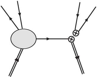
Figure 7: Nonperturbative charming penguin contribution to the forward scattering amplitude. The blob is the nonperturbative charm contribution and the mirror image is omitted.

For pseudoscalar or longitudinally polarized vector meson, on the other hand, the nonperturbative charming penguin contribution is

$$\begin{split}\mathcal{T}_{c\overline{c}}=&8\int\frac{dn\cdot k\,d\overline{n}\cdot z}{4\pi}i\!\int d^{4}y~{}e^{i[m_{b}(1-x_{M})-n\cdot k]\overline{n}\cdot z/2}e^{+in\cdot k\overline{n}\cdot y/2}J_{m_{b}}(n\cdot k+i\epsilon)\\ &\times\langle B_{v}|\mathrm{T}\overline{b}_{v}Y_{n}(\tfrac{\overline{n}\cdot z}{2})\gamma_{\perp}^{\mu}\frac{{\overline{n}}\!\!\!/}{2}\gamma^{\nu}P_{L}T^{a}Y_{\overline{n}}^{\dagger}c_{-v_{\bar{c}c}}(0)\\ &\times\overline{c}_{-v_{\bar{c}c}}Y_{\overline{n}}\gamma^{\perp}_{\mu}T^{a}Y_{n}^{\dagger}c_{v_{\bar{c}c}}(y)\cdot\bar{c}_{v_{\bar{c}c}}Y_{n}\gamma_{\nu}P_{L}Y_{n}^{\dagger}b_{v}(0)|B_{v}\rangle.\end{split}$$ (102)

The factorization in $\mathcal{T}_{c\overline{c}}$ is more apparent if we rewrite it in a more compact form as

$$\mathcal{T}_{c\overline{c}} = -2\int^{\overline{\Lambda}}_{-m_{b}(1-x_{M})}dn\cdot l\;f_{c\overline{c}}^{(1)}\big{(}m_{b}(1-x_{M})+n\cdot l,n\cdot l\big{)}\;J_{m_{b}}(n\cdot k+i\epsilon)$$ (103)

where we have introduced a new, in general complex, nonperturbative function $f_{c\bar{c}}^{(1)}$

$$\begin{split}\int^{\overline{\Lambda}}_{-m_{b}(1-x_{M})}&dn\cdot l~{}e^{in\cdot l\overline{n}\cdot z/2}f_{c\overline{c}}^{(1)}(n\cdot k,n\cdot l)=\\ &-2i\!\int d^{4}y~{}e^{in\cdot k\overline{n}\cdot y/2}\langle B_{v}|\mathrm{T}\big{[}(\overline{b}_{v}Y_{n})(\tfrac{\overline{n}\cdot z}{2})\gamma_{\perp}^{\mu}{\overline{n}}\!\!\!/\gamma^{\nu}P_{L}T^{a}(Y_{\overline{n}}^{\dagger}c_{-v_{\bar{c}c}})(0)\big{]}\\ &\times\big{[}\overline{c}_{-v_{\bar{c}c}}Y_{\overline{n}}\gamma^{\perp}_{\mu}T^{a}Y_{n}^{\dagger}c_{v_{\bar{c}c}}\big{]}(y)\big{[}\bar{c}_{v_{\bar{c}c}}Y_{n}^{\dagger}\gamma_{\nu}P_{L}Y_{n}^{\dagger}b_{v}\big{]}(0)|B_{v}\rangle.\end{split}$$ (104)

The integration over $n\cdot l$ can be interpreted as the integration over soft fluctuations of $b_{v}$. Taking the discontinuity of the jet function in $\mathcal{T}_{c\overline{c}}$ we finally obtain

$$\mathcal{F}_{c\overline{c}}^{(1)}=2\int^{\overline{\Lambda}}_{-m_{b}(1-x_{M})}dn\cdot l\;f_{c\overline{c}}^{(1)}\big{(}m_{b}(1-x_{M})+n\cdot l,n\cdot l\big{)}\;\Big{[}-\frac{1}{\pi}\mathrm{Im}\ J_{m_{b}}(n\cdot k+i\epsilon)\Big{]}.$$ (105)

The jet function can be systematically computed in powers of $\alpha_{s}(\sqrt{\Lambda m_{b}})$. Instead of pursuing this option, we can treat the convolution of jet function and $f_{c\overline{c}}^{(1)}$ as a nonperturbative function to be determined from experiment. The nonperturbative charming penguin contribution to the decay rate corresponding to a sum of Fig. 7 and its mirror image is then

$$\begin{split}\frac{d\Gamma^{(1)}_{c\overline{c}}(B\to MX)}{dE_{M}}=&16\pi^{2}\alpha_{s}(2m_{c})\frac{G_{F}^{2}}{N}\frac{f_{M}^{2}E_{M}^{3}}{16\pi^{2}}\frac{1}{8r^{2}m_{b}^{2}}~{}\phi_{M}(1-{4r^{2}}/{x_{M}})\\ &\times\lambda_{c}^{(q)}c_{q}^{BM}C_{1}(m_{b})\cdot 2\mathrm{Re}\Bigl{[}\mathcal{T}_{M}^{(q)*}(m_{b})\mathcal{F}_{c\overline{c}}^{(1)}(x_{M})\Bigr{]}.\end{split}$$ (106)

If we include all the possible contributions from the four-quark operators, the nonperturbative charming penguin contribution to the decay rate at leading order in $1/m_{c,b}$ and $\alpha_{s}(2m_{c})$ is written as

$$\frac{d\Gamma_{\bar{c}c}(B\to XM)}{dE_{M}}=\frac{G_{F}^{2}}{8\pi}f_{M}^{2}m_{b}^{2}x_{M}^{3}\alpha_{s}(2m_{c})\lambda_{c}^{(q)}c_{q}^{BM}\phi_{M}(1-{4r^{2}}/{x_{M}})\cdot 2\mathrm{Re}\mathcal{T}_{M}^{(q)*}\mathcal{F}_{c\overline{c}},$$ (107)

where the hard coefficients $\mathcal{T}_{M}^{(q)}$ are listed in Table 1, while

$$\mathcal{F}_{c\overline{c}} = \frac{\pi}{8Nr^{2}m_{b}}\left\{\left[C_{1}(m_{b})+C_{4}(m_{b})+C_{10}(m_{b})\right]\mathcal{F}_{c\overline{c}}^{(1)}\right.+\left[C_{2}(m_{b})+C_{3}(m_{b})+C_{9}(m_{b})\right]\mathcal{F}_{c\overline{c}}^{(2)}$$ (108)

$$+ \lambda_{u}^{(q)}/\lambda_{c}^{(q)}\left.\left[\big{(}C_{4}(m_{b})+C_{10}(m_{b})\big{)}\mathcal{F}_{c\overline{c}}^{(1)}+\big{(}C_{3}(m_{b})+C_{9}(m_{b})\big{)}\mathcal{F}_{c\overline{c}}^{(2)}\right]\right\}.$$

The nonperturbative function $\mathcal{F}_{c\overline{c}}^{(2)}$ arises from the weak operators with the same color structure as $O_{2}^{c}$, so that

$$\mathcal{F}_{c\overline{c}}^{(2)}=2\int^{\overline{\Lambda}}_{-m_{b}(1-x_{M})}dn\cdot l\;f_{c\overline{c}}^{(2)}\big{(}m_{b}(1-x_{M})+n\cdot l,n\cdot l\big{)}\;\Big{[}-\frac{1}{\pi}\mathrm{Im}\ J_{m_{b}}(n\cdot k+i\epsilon)\Big{]},$$ (109)

where

$$\begin{split}\int^{\overline{\Lambda}}_{-m_{b}(1-x_{M})}&dn\cdot l~{}e^{in\cdot l\overline{n}\cdot z/2}f_{c\overline{c}}^{(2)}(n\cdot k,n\cdot l)=\\ &-2i\int d^{4}y~{}e^{+in\cdot k\overline{n}\cdot y/2}\langle B_{v}|\mathrm{T}\overline{b}_{v}Y_{n}(\tfrac{\overline{n}\cdot z}{2})\gamma_{\perp}^{\mu}{\overline{n}}\!\!\!/\gamma^{\nu}P_{L}T^{a}Y_{\overline{n}}^{\dagger}b_{v}(0)\\ &\times\overline{c}_{-v_{\bar{c}c}}Y_{\overline{n}}\gamma^{\perp}_{\mu}T^{a}Y_{n}^{\dagger}c_{v_{\bar{c}c}}(y)\cdot\bar{c}_{v_{\bar{c}c}}Y_{n}^{\dagger}\gamma_{\nu}P_{L}Y_{n}^{\dagger}c_{-v_{\bar{c}c}}(0)|B_{v}\rangle.\end{split}$$ (110)

The terms proportional to $\lambda_{u}^{(q)}$ in (108) are smaller than $<2\%\ (<0.1\%)$ of the terms in the first row of (108) for $\Delta S=0\ (\Delta S=1)$ decays and can be safely neglected.

The function $\mathcal{F}_{c\overline{c}}$ is independent of the outgoing meson $M$. In obtaining Eq. (107) an expansion in $\alpha_{s}(2m_{c})$ was used. If the expansion does not converge one can still parametrize the nonperturbative charming penguins by treating the product of $\alpha_{s}(2m_{c})$, the LCDA, and $\mathcal{F}_{c\overline{c}}$ as a new nonperturbative parameter, to be extracted from experiment. Unlike $\mathcal{F}_{c\overline{c}}$, however, this new parameter depends on $M$.

References

• (1) T. E. Browder, A. Datta, X. G. He and S. Pakvasa, Phys. Rev. D 57, 6829 (1998); A. Datta, X. G. He and S. Pakvasa, Phys. Lett. B 419, 369 (1998); X. G. He, C. P. Kao, J. P. Ma and S. Pakvasa, Phys. Rev. D 66, 097501 (2002).
• (2) D. Atwood and A. Soni, Phys. Rev. Lett.  79, 5206 (1997).
• (3) A. L. Kagan and A. A. Petrov, arXiv:hep-ph/9707354.
• (4) X. G. He and G. L. Lin, Phys. Lett. B 454, 123 (1999); X. G. He, J. P. Ma and C. Y. Wu, Phys. Rev. D 63, 094004 (2001); X. G. He, C. Jin and J. P. Ma, Phys. Rev. D 64, 014020 (2001).
• (5) X. Calmet, T. Mannel and I. Schwarze, Phys. Rev. D 61, 114004 (2000); X. Calmet, T. Mannel and I. Schwarze, Phys. Rev. D 62, 096014 (2000); X. Calmet, Phys. Rev. D 62, 014027 (2000); X. Calmet, Phys. Rev. D 62, 016011 (2000).
• (6) H. Y. Cheng and A. Soni, Phys. Rev. D 64, 114013 (2001).
• (7) C. S. Kim, J. Lee, S. Oh, J. S. Hong, D. Y. Kim and H. S. Kim, Eur. Phys. J. C 25, 413 (2002).
• (8) G. Eilam and Y. D. Yang, Phys. Rev. D 66, 074010 (2002).
• (9) A. Soni and J. Zupan, arXiv:hep-ph/0510325.
• (10) C. W. Bauer, S. Fleming and M. E. Luke, Phys. Rev. D 63, 014006 (2001).
• (11) C. W. Bauer, S. Fleming, D. Pirjol and I. W. Stewart, Phys. Rev. D 63, 114020 (2001).
• (12) C. W. Bauer and I. W. Stewart, Phys. Lett. B 516, 134 (2001).
• (13) C. W. Bauer, D. Pirjol and I. W. Stewart, Phys. Rev. D 65, 054022 (2002).
• (14) J. Chay and C. Kim, Phys. Rev. D 68, 071502 (2003).
• (15) J. Chay and C. Kim, Nucl. Phys. B 680, 302 (2004).
• (16) J. Chay, A. K. Leibovich, C. Kim, J. Zupan, work in progress.
• (17) C. W. Bauer and A. V. Manohar, Phys. Rev. D 70, 034024 (2004); S. W. Bosch, B. O. Lange, M. Neubert and G. Paz, Nucl. Phys. B 699, 335 (2004); M. Neubert, Eur. Phys. J. C 40, 165 (2005).
• (18) M. Ciuchini, E. Franco, G. Martinelli and L. Silvestrini, Nucl. Phys. B 501, 271 (1997); M. Ciuchini, E. Franco, G. Martinelli, M. Pierini and L. Silvestrini, Phys. Lett. B 515, 33 (2001).
• (19) C. W. Bauer, D. Pirjol, I. Z. Rothstein and I. W. Stewart, Phys. Rev. D 70, 054015 (2004); C. W. Bauer, I. Z. Rothstein and I. W. Stewart, arXiv:hep-ph/0510241.
• (20) A. R. Williamson and J. Zupan, arXiv:hep-ph/0601214.
• (21) M. Beneke, G. Buchalla, M. Neubert and C. T. Sachrajda, Phys. Rev. Lett.  83, 1914 (1999); M. Beneke, G. Buchalla, M. Neubert and C. T. Sachrajda, Nucl. Phys. B 591, 313 (2000); M. Beneke, G. Buchalla, M. Neubert and C. T. Sachrajda, Nucl. Phys. B 606, 245 (2001); M. Beneke and M. Neubert, Nucl. Phys. B 675, 333 (2003).
• (22) C. W. Bauer, D. Pirjol, I. Z. Rothstein and I. W. Stewart, Phys. Rev. D 72, 098502 (2005).
• (23) M. Beneke, G. Buchalla, M. Neubert and C. T. Sachrajda, Phys. Rev. D 72, 098501 (2005).
• (24) G. P. Korchemsky and G. Sterman, Phys. Lett. B 340, 96 (1994); R. Akhoury and I. Z. Rothstein, Phys. Rev. D 54, 2349 (1996).
• (25) G. P. Lepage and S. J. Brodsky, Phys. Rev. D 22, 2157 (1980).
• (26) V. L. Chernyak and A. R. Zhitnitsky, Phys. Rept.  112, 173 (1984).
• (27) S. Fleming and A. K. Leibovich, Phys. Rev. D 70, 094016 (2004).
• (28) V. M. Braun, G. P. Korchemsky and D. Mueller, Prog. Part. Nucl. Phys.  51, 311 (2003).
• (29) J. Chay, C. Kim and A. K. Leibovich, Phys. Rev. D 72, 014010 (2005).
• (30) T. Feldmann and T. Hurth, JHEP 0411, 037 (2004).
• (31) C. W. Bauer, M. E. Luke and T. Mannel, Phys. Rev. D 68, 094001 (2003).
• (32) A. K. Leibovich, Z. Ligeti and M. B. Wise, Phys. Lett. B 539, 242 (2002).
• (33) C. W. Bauer, M. Luke and T. Mannel, Phys. Lett. B 543, 261 (2002).
• (34) K. S. M. Lee and I. W. Stewart, Nucl. Phys. B 721, 325 (2005).
• (35) S. W. Bosch, M. Neubert and G. Paz, JHEP 0411, 073 (2004).
• (36) J. Chay and C. Kim, Phys. Rev. D 65, 114016 (2002).
• (37) A. V. Manohar, T. Mehen, D. Pirjol and I. W. Stewart, Phys. Lett. B 539, 59 (2002).
• (38) A. Hardmeier, E. Lunghi, D. Pirjol and D. Wyler, Nucl. Phys. B 682, 150 (2004).
• (39) A. K. Leibovich, Z. Ligeti and M. B. Wise, Phys. Lett. B 564, 231 (2003).
• (40) I. Z. Rothstein, Phys. Rev. D 70, 054024 (2004).
• (41) J. W. Chen and I. W. Stewart, Phys. Rev. Lett.  92, 202001 (2004).
• (42) A. Khodjamirian, T. Mannel and M. Melcher, Phys. Rev. D 68, 114007 (2003); V. M. Braun and A. Lenz, Phys. Rev. D 70, 074020 (2004); P. Ball and R. Zwicky, JHEP 0602, 034 (2006).
• (43) P. Ball, V. M. Braun and A. Lenz, JHEP 0605, 004 (2006).
• (44) P. Ball and R. Zwicky, Phys. Rev. D 71, 014029 (2005).
• (45) P. Ball and R. Zwicky, Phys. Rev. D 71, 014015 (2005).
• (46) C. W. Bauer, D. Pirjol and I. W. Stewart, Phys. Rev. D 68, 034021 (2003).
• (47) B. Aubert et al. [BABAR Collaboration], Phys. Rev. Lett.  91, 171802 (2003).
• (48) B. Aubert et al. [BABAR Collaboration], Phys. Rev. Lett.  93, 231804 (2004).
• (49) K. Abe et al. [BELLE Collaboration], arXiv:hep-ex/0408141.
• (50) P. Colangelo, F. De Fazio and T. N. Pham, Phys. Lett. B 597, 291 (2004); M. Ladisa, V. Laporta, G. Nardulli and P. Santorelli, Phys. Rev. D 70, 114025 (2004); H. Y. Cheng, C. K. Chua and A. Soni, Phys. Rev. D 71, 014030 (2005).
• (51) A. L. Kagan, Phys. Lett. B 601, 151 (2004).
• (52) H. n. Li, arXiv:hep-ph/0411305; H. n. Li and S. Mishima, Phys. Rev. D 71, 054025 (2005).