QCD Factorization for Deep-Inelastic Scattering
At Large Bjorken $x_{B}\sim 1-{\cal O}(\Lambda_{\rm QCD}/Q)$

Abstract

We study deep-inelastic scattering factorization on a nucleon in the end-point regime $x_{B}\sim 1-{\cal O}(\Lambda_{\rm QCD}/Q)$ where the traditional operator product expansion is supposed to fail. We argue, nevertheless, that the standard result holds to leading order in $1-x_{B}$ due to the absence of the scale dependence on $(1-x_{B})Q$. Refactorization of the scale $(1-x_{B})Q^{2}$ in the coefficient function can be made in the soft-collinear effective theory and remains valid in the end-point regime. On the other hand, the traditional refactorization approach introduces the spurious scale $(1-x_{B})Q$ in various factors, which drives them nonperturbative in the region of our interest. We show how to improve the situation by introducing a rapidity cut-off scheme, and how to recover the effective theory refactorization by choosing appropriately the cut-off parameter. Through a one-loop calculation, we demonstrate explicitly that the proper soft subtractions must be made in the collinear matrix elements to avoid double counting.

I Introduction

In lepton-nucleon deep-inelastic scattering (DIS), the Bjorken regime with virtual photon mass $Q^{2}\rightarrow\infty$ and $x_{B}=Q^{2}/2M\nu$ fixed presents a textbook example of perturbative QCD (pQCD) factorization collins89 . In this regime, the scale $(1-x)^{\alpha}Q$ goes to infinity (we drop the subscript $B$ on $x$ henceforth), where $\alpha$ is any real number, or at least much larger than the soft QCD scale $\Lambda_{\rm QCD}$. An alternative DIS regime is $Q^{2}\rightarrow\infty$ with $(1-x)Q\sim\Lambda_{\rm QCD}$, where the final hadron state invariant mass $(1-x)Q^{2}\sim Q\Lambda_{\rm QCD}$ is still large and is distinct from the resonance region. This large-$x$ regime has so far received little attention in theory, possibly because it covers only a small kinematic interval in real experiments. The existing QCD studies in the literature are somewhat controversial kim ; pecjak .

In this paper, we present a factorization study of DIS at this regime. The main point we advocate here is that the standard pQCD factorization remains valid in this new kinematic domain to leading order in $1-x$. Then we move on to discuss refactorization which factorizes the physics at scale $(1-x)Q^{2}$ from that at $Q^{2}$. The useful theoretical framework for this purpose is the so-called soft-collinear effective field theory (SCET) developed recently SCET . Indeed, the first treatment of the large-$x$ region in DIS using SCET was made in manohar and followed in kim ; pecjak for $(1-x)Q\sim\Lambda_{\rm QCD}$ [see also neu .] Because the scale $(1-x)Q$ does not enter in the perturbative calculation, the final result amounts to a standard pQCD factorization, with the additional benefit that the refactorization becomes manifest. One subtlety we discuss extensively in this paper is the role of the soft contribution and its relation to the light-cone parton distribution. In a recent paper kim , a factorization formula for the DIS structure function is derived in SCET, which is similar to what we find here. However, because of the lack of a consistent regularization and clear separation of contributions among different factors, the result does not recover that of Ref. manohar in the limit $(1-x)Q\gg\Lambda_{QCD}$.

The traditional approach of refactorization was pioneered in sterman , where a new parton distribution together with soft factor and jet function is introduced. These matrix elements are designed to absorb large logarithms generated from soft gluon radiations off on-shell lines. Evolution equations for them are derived and solved to resum the large soft-gluon logarithms. In this approach, the factorization of scales are not apparent from the start. Moreover, a spurious scale $(1-x)Q$ appears in all factors which makes them nonperturbative in the regime of our interest. After reviewing this, we present a more general factorization along this line with dependence on a rapidity cut-off $\rho$. Different choices of the cutoff lead to redistributions of large logarithms in different matrix elements. A particular choice yields a picture similar to that of the SCET approach.

The presentation of this paper is as follows. In section II, we argue that the standard factorization approach remains valid in the end-point regime $x\sim 1-{\cal O}(\Lambda_{\rm QCD}/Q)$. In section III, we present an effective field theory approach to refactorization, following the previous work of Ref. kim . The difference is that our result is consistent with that of Ref. manohar , with the jet factor absorbing all physics at the intermediate scale $(1-x)Q^{2}$. We explain that the soft and collinear contributions combine to give the light-cone parton distribution. In section IV, we first review the traditional factorization in which various matrix elements are introduced to account for soft gluon radiations. We then show how to derive a more general factorization with a rapidity cutoff. We demonstrate explicitly that the proper soft subtractions must be made in the collinear matrix elements to avoid double counting. By choosing different cut-off, we find different pictures of factorization and large-logarithmic resummation. The effective field theory refactorization can be recovered this way.

II Validity of the standard QCD factorization at $x_{B}\sim 1-{\cal O}(\Lambda_{\rm QCD}/Q)$

The standard pQCD factorization theorem is derived in the Bjorken limit in which $Q^{2}\rightarrow\infty$ and $x$ is a fixed constant between $0$ and $1$. To leading order in $1/Q^{2}$, the proton’s spin-independent structure function $F_{1}(x,Q^{2})$ can be factorized as

$$F_{1}(x,Q^{2})=\sum_{f}\int^{1}_{x}\frac{dy}{y}C_{f}\left(\frac{x}{y},\frac{Q^{2}}{\mu^{2}}\right)q_{f}(y,\mu^{2})\ ,$$ (1)

where $\mu$ is a factorization scale, $C_{f}$ is the coefficient function depending on scale $Q^{2}$ and $\mu^{2}$ (factorization scale), and $q_{f}$ is a quark distribution of flavor $f$. For simplicity, we omit the quark charges and gluon contribution which are inessential for our discussion. In the moment space, the factorization takes a simple product form,

$$F_{1}^{N}(Q^{2})=\sum_{f}C_{fN}(Q^{2}/\mu^{2})q_{fN}(\mu^{2})\ ,$$ (2)

where the moments are defined the usual way, e.g., $q_{N}=\int^{1}_{0}dxx^{N-1}(q(x)+\bar{q}(x))$ with $N$ even.

The above factorization in principle is invalid in non-Bjorken regions. However, we argue that it still holds in the regime of our interest, $(1-x)Q\sim\Lambda_{\rm QCD}$, with the same physical parton distributions to leading order in $1-x$. The main point is that although we now have a new infrared scale $(1-x)Q$, it does not appear in the above factorization.

Indeed, as $x\rightarrow 1$ the coefficient function $C_{f}$ can only depend on the two hard scales—invariant photon mass $Q^{2}$ and the final-hadron-state invariant mass $(1-x)Q^{2}$, both remain large when $(1-x)Q\sim\Lambda_{\rm QCD}$. Hence there is no emerging infrared scale entering physical observables in this new regime, and the original factorization remains valid to leading order in $1-x$.

The above observation can be seen clearly in the one-loop result. The coefficient function at order $\alpha_{s}$ in the $x$-space

$$C^{(1)}(x)=\frac{\alpha_{s}}{2\pi}C_{F}\left[\left(\frac{2\ln((1-x)Q^{2}/\mu^{2})-3/2}{1-x}\right)_{+}-\left(\frac{3}{2}\ln\frac{Q^{2}}{\mu^{2}}+\frac{9}{2}+\frac{\pi^{2}}{3}\right)\delta(1-x)\right]\ ,$$ (3)

where we have neglected higher order in $(1-x)$. The scheme we use here is the modified minimal subtraction (${\overline{\rm MS}}$). In term of moments, one finds

$$C_{N}^{(1)}\left(\frac{Q^{2}}{\mu^{2}},\frac{Q^{2}}{N\mu^{2}}\right)=\frac{\alpha_{s}}{2\pi}C_{F}\left[\ln^{2}\frac{Q^{2}}{N\mu^{2}}-\frac{3}{2}\ln\frac{Q^{2}}{N\mu^{2}}-\ln^{2}\frac{Q^{2}}{\mu^{2}}+3\ln\frac{Q^{2}}{\mu^{2}}-\frac{9}{2}-\frac{\pi^{2}}{6}\right]\ .$$ (4)

The scale dependence is manifest: The first two logarithms come from physics at scale $\mu^{2}=Q^{2}/N$, whereas the next two logarithms come from scale $Q^{2}$. Clearly, there is no physics from scale $\mu^{2}\sim(1-x)^{2}Q^{2}\sim Q^{2}/N^{2}$. Therefore, even when $(1-x)Q$ becomes of order $\Lambda_{\rm QCD}$, the coefficient function has no infrared sensitivity to it.

The fundamental reason for the absence of the scale $(1-x)Q$ in a physical observable is that it is not a Lorentz scalar, whereas $(1-x)Q^{2}$ is the invariant mass of the final hadron state. In principle, the energy of soft gluons and quarks in the Breit frame is of order $(1-x)Q$ which can appear in the factorization. However, this happens only for frame-dependent factorization. The factorization we quoted above is frame-independent and thus any non-Lorentz scalar cannot appear.

Although the above conclusion appears simple and natural, we have not seen it stated explicitly in the literature.

III Refactorization: Effective Theory Approach

In the large-$x$ region, independent of whether $(1-x)Q\gg\Lambda_{\rm QCD}$ or $\sim\Lambda_{\rm QCD}$, there is an emerging “infrared” scale $(1-x)Q^{2}\ll Q^{2}$. Of course, we always assume $(1-x)Q^{2}\gg\Lambda_{\rm QCD}^{2}$. The presence of this new scale suggests a further factorization in which the physics associated with scales $Q^{2}$ and $(1-x)Q^{2}$ is disentangled. This type of factorization was proposed by G. Sterman and others for the purpose of summing over the large double logarithms of type $\alpha_{s}^{k}[\ln^{i}(1-x)/(1-x)]_{+}$ $(i\leq 2k-1)$ in the coefficient functions sterman . We consider this refactorization in this and the following sections, commenting on its applicability in the region of our interest.

We first study refactorization in the effective field theory (EFT) approach in this section, and will discuss a more intuitive approach in the next. The EFT method is based on strict scale separation, very much like the usual QCD factorization discussed in the previous section. When the scales are separated, one can sum over large logarithms by using renormalization group evolutions between scales. Some of the basic discussions here follow Refs. manohar ; ji ; kim .

III.1 EFT Refactorization

To understand the EFT factorization heuristically, we write the one-loop coefficient function in Eq. (4) in a factorized form,

$$C_{N}^{(1)}\left(\frac{Q^{2}}{\mu^{2}},\frac{Q^{2}}{\overline{N}\mu^{2}}\right)=2C^{(1)}\left(\frac{Q^{2}}{\mu^{2}}\right)+{\cal M}_{N}^{(1)}\left(\frac{Q^{2}}{{\overline{N}}\mu^{2}}\right)\ ,$$ (5)

where $C^{(1)}$ is $N$-independent and comes from physics at scale $Q^{2}$ and ${\overline{N}}=Ne^{\gamma_{E}}$ where $\gamma_{E}$ is Euler constant. The one-loop result for $C$ is

$$C^{(1)}\left(\frac{Q^{2}}{\mu^{2}}\right)=\frac{\alpha_{s}}{4\pi}C_{F}\left[-\ln^{2}\frac{Q^{2}}{\mu^{2}}+3\ln\frac{Q^{2}}{\mu^{2}}-8+\frac{\pi^{2}}{6}\right]\ ,$$ (6)

where the constant term is, in principle, arbitrary; we choose it to be consistent with the effective current below. The two-loop result for $C$ can be found in feng ; idi . The other factor ${\cal M}_{N}^{(1)}$ comes entirely from physics at scale $(1-x)Q^{2}\sim Q^{2}/\overline{N}$,

$${\cal M}_{N}^{(1)}\left(\frac{Q^{2}}{{\overline{N}}\mu^{2}}\right)=\frac{\alpha_{s}}{2\pi}C_{F}\left[\ln^{2}\frac{Q^{2}}{{\overline{N}}\mu^{2}}-\frac{3}{2}\ln\frac{Q^{2}}{{\overline{N}}\mu^{2}}+\frac{7}{2}-\frac{\pi^{2}}{3}\right]\ ,$$ (7)

and the second order result for ${\cal M}_{N}$ can also be found in idi . The key point is that the above refactorization of scales works to all orders in perturbation theory and EFT provides a formal approach to establish this: The physics at scale $Q^{2}$ can be included entirely in $|C|^{2}$ and that at the other scale is in ${\cal M}_{N}$.

To arrive at the above refactorization, we start off at the scale $Q^{2}$ at which perturbative physics involves virtual gluon corrections to the hard interaction photon vertex. Note that the soft-gluon radiations off a hard vertex are usually high-order effects in $1/Q^{2}$ and can be neglected. Thus the physics at $Q^{2}$ can be found from just the quark electromagnetic form factor. Integrating out physics at scale $Q^{2}$ is equivalent to matching the full QCD electromagnetic current to an effective one involving just soft-collinear physics.

$$J_{\rm QCD}^{\mu}=C(Q^{2}/\mu^{2})J_{\rm eff}^{\mu}(Q^{2}/\mu^{2})\ ,$$ (8)

with the one-loop result given in Eq. (6).

We can run the effective current from scale $Q^{2}$ to scale $(1-x)Q^{2}$ using the renormalization group equation

$$\mu\frac{dJ_{\rm eff}(Q^{2}/\mu^{2})}{d\mu}=-\gamma_{1}(\alpha_{s}(\mu))J_{\rm eff}(Q^{2}/\mu^{2})\ ,$$ (9)

where the anomalous dimension can be calculated from $C$, $\gamma_{1}=\mu d\ln C/d\mu$, and has the following generic form,

$$\gamma_{1}=A(\alpha_{s})\ln Q^{2}/\mu^{2}+B_{1}(\alpha_{s})\ ,$$ (10)

in which $A$ and $B_{1}$ are a series in strong coupling constant $\alpha_{s}$ and are now known up to three loops dd .

At scale $\mu_{I}^{2}=(1-x)Q^{2}$, we follow Ref. kim , matching products of the effective currents to a product of the jet function, collinear parton contribution, and soft distribution in SCET. Introducing a small expansion parameter $\lambda$, with $\lambda^{2}Q\sim\Lambda_{\rm QCD}$, $1-x$ in the region of our interest scales like $\lambda^{2}$. The collinear partons at the matching scale $\mu_{I}^{2}$ have momentum $(p^{+},p^{-}p_{\perp})\sim Q(1,\lambda^{4},\lambda^{2})$ [our notation for light-cone components for arbitrary four-vector $l$ is $l\equiv(l^{+},l^{-},l_{\perp})$ with $l^{\pm}=\frac{1}{\sqrt{2}}(l^{0}\pm l^{3})$], and the soft partons have momentum $(\lambda^{2},\lambda^{2},\lambda^{2})Q$. The moment of the structure function $F_{1}$ after the second stage matching has the following form kim ,

$$F_{1}^{N}(Q)=C^{2}(Q^{2}/\mu_{I}^{2})J_{P}(N,Q^{2}/\mu_{I}^{2})\phi_{N}(\mu_{I}^{2})S_{N}(\mu_{I}^{2})\ ,$$ (11)

where various factors are defined as follows.

The jet function $J_{P}(N,\mu^{2}_{I})$ is related to the absorbtive part of the hard collinear quark propagator ${\cal G}_{P}$,

$$\langle 0|T\left[W_{n}^{\dagger}\xi_{n}(z)\bar{\xi}_{n}W_{n}(0)\right]|0\rangle=i\frac{\not\!n}{\sqrt{2}}\int\frac{d^{4}k}{(2\pi)^{4}}e^{-ikz}{\cal G}_{P}(k)\ .$$ (12)

where $\xi_{n}$ is a collinear quark field and $W_{n}$ is a Wilson line along the light-cone direction $\bar{n}$ $(n^{2}=\bar{n}^{2}=0,\bar{n}\cdot n=1)$. A hard collinear quark has momentum $p+k$, where $p$ is the so-called label momentum with $p^{+}\sim Q$ and $k$ is a hard residual momentum with components of order $Q(1,\lambda^{2},\lambda)$. Therefore, the virtuality of the hard-collinear quark is $2p\cdot k\sim\lambda^{2}Q^{2}$, consistent with that of the hadron final state. The jet function has no infrared divergences because the hadron final states are summed over. However, it does have light-cone divergences which are handled by the standard minimal subtraction method. An important feature of the jet function is that it is only sensitive to physics at scale $\mu_{I}^{2}$. In fact, at one-loop order, the jet function reproduces the ${\cal M}_{N}$ function in the previous section.

The soft contribution in Eq. (12) is defined in terms of the soft Wilson lines chay1 : $Y_{n}(x)={\mathcal{P}}\exp[-ig\int^{x}_{-\infty}dsn\cdot A_{\rm us}]$ and $\widetilde{Y}_{n}(x)=\overline{{\mathcal{P}}}\exp[-ig\int^{\infty}_{x}dsn\cdot A_{\rm us}]$, where $A_{\rm us}$ are the so-called ultra-soft gluons with momentum $Q(\lambda^{2},\lambda^{2},\lambda^{2})$ and ${\mathcal{P}}$ stands for path ordering [the sign convention for the gauge coupling is $D^{\mu}=\partial^{\mu}+igA^{\mu}$],

$$S(x,\mu_{I}^{2})=\frac{1}{N_{c}}\left\langle 0\left|{\rm Tr}\left[{Y_{\bar{n}}}^{\dagger}\tilde{Y}_{n}\delta\left(1-x+\frac{n\cdot i\partial}{n\cdot p}\right)\tilde{Y}^{\dagger}_{n}Y_{\bar{n}}\right]\right|0\right\rangle\ ,$$ (13)

where the ratio in the delta function fixes the momentum of the emitted gluon to be soft (of order $\lambda^{2}$). As such, the soft factor is a non-perturbative contribution.

The collinear contribution,

$$\phi(x,\mu_{I}^{2})=\left\langle P\left|\bar{\xi}_{\bar{n}}W_{\bar{n}}\delta\left(x-\frac{n\cdot{\cal P}_{+}}{n\cdot p}\right)\frac{\not\!n}{\sqrt{2}}W^{\dagger}_{\bar{n}}\xi_{\bar{n}}\right|P\right\rangle$$ (14)

comes from collinear quarks and gluons with momentum $(1,\lambda^{2},\lambda)Q$ and $n\cdot{\cal P}_{+}$ is the total light-cone momentum carried by the partons. In Ref. kim , the collinear contribution was identified as the usual Feynman parton distribution. This, however, is incorrect because the soft gluons with longitudinal momentum $(1-x)Q\sim\lambda^{2}$ in the proton cannot be included in the collinear contribution according to the definition of the collinear gluons in SCET. On the other hand, the Feynman parton distribution contains a factorizable soft contribution in the limit $x\rightarrow 1$ korchemsky ; ji1 . Further discussion on this issue will be made in the next subsection as well as in the next section. The correct approach is to combine the soft and collinear contributions together to get the correct Feynman parton distribution in the $x\rightarrow 1$ limit.

Thus EFT arguments lead finally to the following refactorization, valid when $(1-x)Q\sim\Lambda_{\rm QCD}$ at leading order in $1-x$,

$$F_{1}^{N}(Q^{2})=C^{2}(Q^{2}/\mu^{2}_{I})J_{P}(Q^{2}/N\mu_{I}^{2})q_{N}(\mu_{I}^{2})+{\cal O}(1-x),$$ (15)

where $q_{N}(\mu_{I}^{2})$ is the moment of the quark distribution, and the jet function is exactly the ${\cal M}_{N}$ function introduced in the previous section. Although formally this factorization is made at $\mu_{I}^{2}$, the product of factors is independent of it. The claim of non-factorizability of DIS in this very regime in Ref. pecjak was criticized in manohar1 . On the other hand, the above result seems consistent with that of Ref. neu if used in the same regime.

The above factorization allows us to resum over large logarithms. Since the physical structure function is $\mu$-independent, we can take $\mu_{I}$ in the above expression to whatever value we choose. For example, if one sets $\mu^{2}_{I}=Q^{2}$, all large logarithms are now included in the jet function. One can derive a renormalization group equation for $J_{P}$ manohar . Solving this equation leads to a resummation of large logarithms.

Alternatively, with the original scale $\mu_{I}^{2}$, there are large logarithms in $C$, which can be resummed using the renormalization group equation and the anomalous dimension $\gamma_{1}$. The resulting exponential evolution can be regarded as the evolution of the jet function from scale $Q^{2}$ to $\mu_{I}^{2}$. The parton distribution $q_{N}(\mu_{I})$ runs from $\mu_{I}^{2}$ to a certain factorization scale $\mu_{F}^{2}$ using the DGLAP evolution dglap . This running generates the logarithms from initial-state parton radiations.

In the above refactorization, no scale $(1-x)Q$ appears explicitly although soft and collinear gluons in SCET do have reference to that scale. This explains that the factorization holds in the region of our interest, namely, when $(1-x)Q\sim\Lambda_{\rm QCD}$.

III.2 Collinear Contribution in SCET and Double Counting

SCET is an operator approach designed to take into account contributions from different regions in Feynman integrals. Calculations in SCET are sometimes formal if without a careful definition of regulators for individual contributions. Occasionally, the regulators in different parts must be defined consistently to obtain the correct answer. Otherwise, one can easily lead to double counting. The same issue has been discussed recently in Ref. zb .

To see the need of consistent regulators in SCET, let us consider the usual quark distribution in the proton. In the full QCD, the quark distribution is defined as

$$q(x)=\frac{1}{2}\int\frac{d\lambda}{2\pi}e^{i\lambda x}\langle P|\overline{\psi}(\lambda n)\not\!ne^{-ig\int^{\lambda}_{0}d\lambda^{\prime}n\cdot A(\lambda^{\prime}n)}\psi(0)|P\rangle\ ,$$ (16)

where $\psi(x)$ and $A(\lambda n)$ are full QCD quark and gluon fields (here we use the vector $n$ with mass-dimension 1). Now suppose the nucleon is moving with a high momentum $Q$ in the $z$ direction. The quarks and gluons in the proton, in general, have large $k^{+}$, and small momentum $k^{-}$ and $k_{\perp}$, in the sense that they are collinear to the proton momentum. Therefore, one may match the full QCD fields in the above expression to the corresponding collinear fields in SCET.

However, the procedure is incomplete for wee gluons with $(1-x)\sim\Lambda/Q$. Such a gluon has a soft longitudinal momentum and is definitely included in the above gauge link. The QCD factorization theorem shows that soft gluons do not make a singular contribution to the parton density, but it does not exclude the non-singular wee gluon contributions of type $[\ln^{k}(1-x)/(1-x)]_{+}$. In fact, the wee gluon effect in the $x\rightarrow 1$ limit can be factorized out into a soft factor $S(x)$, which is responsible for the large-$x$ behavior of the parton distribution korchemsky ; ji1 . Therefore, in SCET it is natural to express $q(x)$ in terms of the product of the soft factor and true collinear gluon contribution.

In Ref. kim , the evolution equation was derived for the collinear contribution $\phi(x)$ and is found to be the same as the DGLAP evolution, even in the $x\rightarrow 1$ limit. This could be the main motivation to identify $\phi(x)$ as $q(x)$. However, the collinear gluons in the one-loop Feynman diagrams can no longer be considered as “collinear” if $(1-x)Q\sim\Lambda_{\rm QCD}$, and must be subtracted explicitly. This subtraction was not made through certain regulators and hence there is a double counting. In fact, once the soft-gluons are subtracted, a collinear parton jet shall not have singularity in the limit $x\rightarrow 1$. Likewise, the calculation of the soft-factor in Ref. kim should have a soft transverse-momentum cutoff to include just the true soft gluons. Thus, the regulators in the soft and collinear contributions must be made consistently to avoid double counting. A consistent scheme of defining the soft and collinear contributions for a parton distribution defined with off light-cone gauge link can be found in Ref. korchemsky . We will present another example of a consistent regularization in the following section.

IV ReFactorization: Intuitive Approach

The EFT approach for refactorization is gauge-invariant and all factors are defined at separate scales. The resummation is of the simple renormalization-group type. However, the physical origin of the large logarithms is not entirely transparent. For example, it is well known in QED that the double infrared logarithms are generated from soft radiations from jet-like lines. This is not obvious in the EFT approach.

In the approach introduced by Sterman and others sterman , the structure functions are factorized into different factors which have clear physical significance, although each factor now contains multi-scales. Explicit equations can be derived to bridge the scales within these factors, which allow one to resum large logarithms. The main shortcoming of this intuitive approach is the introduction of a spurious scale $(1-x)Q$ in each factor, which make them nonperturbative in the kinematic region of our interest.

In this section, we first briefly review Sterman’s approach in subsection A. We then introduce in subsection B a more general factorization approach along this direction, which involves a rapidity cutoff. With an appropriate cutoff, we arrive at a picture similar to that of EFT. The example also shows that a consistent soft subtraction must be made to obtain a correct factorization.

IV.1 Sterman’s Method

Consider the lepton-nucleon DIS process in the Breit frame in which the initial and final partons have similar momentum but move in opposite directions. In the region $x\rightarrow 1$, the final hadron state consists of a high-energy jet plus soft gluon radiations. A so-called reduced diagram is shown in Fig. 1, showing the space-time picture of the process. There are in principle four different scales which are relevant: virtual photon mass $Q^{2}$, final-hadron invariant mass $(1-x)Q^{2}$, the soft parton energy radiated off the proton $(1-x)Q$, and finally the genuine nonperturbative QCD scale $\Lambda_{\rm QCD}$.

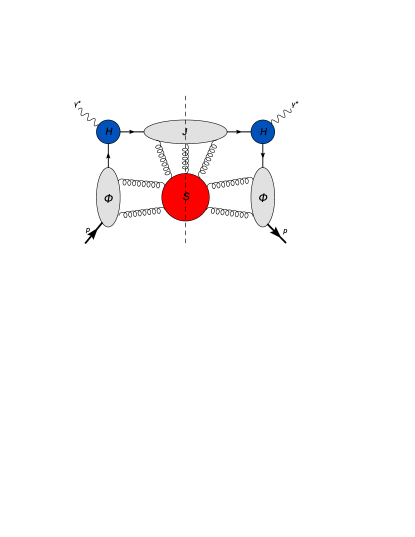
Figure 1: The leading reduced diagram contributing to the deep-inelastic structure function in $x\rightarrow 1$ regime.

According to the analysis in Ref. sterman , the reduced diagram can be factorized into various physically intuitive contributions, and the structure function can be expressed as a product of a soft factor, a final-state jet function, and a parton distribution,

$$F_{1}(x,Q^{2})=H(Q^{2})\int^{1}_{x}\frac{dy}{y}\phi(y)\int^{y-x}_{0}\frac{dw}{1-w}S(w)J(x,y,w)\ .$$ (17)

The parton distribution $\phi(x)$ is not the usual gauge-invariant one on the light-cone. Rather it is defined as

$$\phi(y)=\frac{1}{2p^{+}}\int\frac{d\lambda}{2\pi}e^{-iy\lambda}\langle P|\overline{q}(\lambda n)\gamma^{+}q(0)|P\rangle\ ,$$ (18)

in $A^{z}=0$ gauge, or equivalently there are gauge links along the $z$ direction going from the quark positions to infinity. Because it is not truly gauge-invariant, it is frame-dependent. In particular, it can depend on the soft parton energy $(1-x)Q$. This parton distribution contains contributions of both collinear and soft gluon radiations form the initial state quark, thus involving double logarithms.

Likewise, the jet function is defined as

$$J\sim{\rm Disc}\int\frac{d^{4}x}{(2\pi)^{4}}e^{-ixl}\langle 0|T\left[\overline{q}(x)q(0)\right]|0\rangle$$ (19)

and normalized to $\delta(1-x)$ at the leading order. Once again the jet is defined in the axial gauge and is frame dependent. In particular, it depends on the infrared scale $(1-x)Q$ as well. However, this jet function contains no true infrared divergences. It accounts for the collinear and soft radiations from the jet final state.

Finally, the soft function $S$ is defined as the matrix element of Wilson lines first going along the $\bar{n}$ direction from $-\infty$ along the light-cone, then going along $n$ direction to $+\infty$. The collinear divergences are regularized by $A^{z}=0$ gauge. Therefore, it contains no true infrared divergences.

In the moment space, the refactorization appears in a simple form,

$$F_{1}^{N}(Q^{2})=H(Q^{2}/\mu^{2})\phi_{N}(Q^{2}/\mu^{2})S_{N}(Q^{2}/\mu^{2})J_{N}(Q^{2}/\mu^{2})\ ,$$ (20)

and $H$ stands for the hard contribution which comes only from virtual diagrams. Again, we emphasize that the factorization follows intuitively from the space-time picture of the reduced diagrams. However, one pays a price for this: the breaking of Lorentz invariance and introduction of a new scale $(1-x)Q$. When this scale becomes of order $\Lambda_{\rm QCD}$, as this is the main interest of the paper, all factors becomes nonperturbative in principle. On the other hand, the scale $(1-x)Q$ is spurious, it should be cancelled out. It is unclear how this is achieved at the nonperturbative level.

The physics of the above factorization is best seen through a one-loop calculation. The parton distribution is

$$\phi(x)=\frac{\alpha_{s}}{\pi}C_{F}\left\{-\frac{1}{\epsilon}P_{qq}(x)+\left[\left(2D_{1}+D_{0}\ln\frac{Q^{2}}{\mu^{2}}\right)-D_{0}-\left(\frac{\pi^{2}}{6}+1\right)\delta(1-x)\right]\right\}\ ,$$ (21)

where $P_{qq}(x)$ is the quark splitting function and

$$D_{i}\equiv\left[\frac{\ln^{i}(1-x)}{1-x}\right]_{+}\,\,\,\,\,i=0,1,2....$$ (22)

Apart from the divergent term which is the same as the Feynman parton distribution, there are extra constant terms which absorb the soft-collinear gluon contribution. Some of these come from the scale $(1-x)^{2}Q^{2}$. In moment space, we have

$$\phi_{N}(x)=1+\frac{\alpha_{s}}{4\pi}C_{F}\left[-\frac{1}{\epsilon}(3-4\ln\overline{N})+\ln^{2}\frac{Q^{2}}{{\overline{N}}^{2}\mu^{2}}-2\ln\frac{Q^{2}}{{\overline{N}}^{2}\mu^{2}}-\ln^{2}\frac{Q^{2}}{\mu^{2}}+2\ln\frac{Q^{2}}{\mu^{2}}-4\right]\ .$$ (23)

One may view the double logarithmic terms as from the initial state radiation. The large logarithms resulting from large scale differences can be summed through an $x$-space evolution equation sterman .

The one-loop jet function is explicit finite,

$$J(x) = \delta(1-x)+\frac{\alpha_{s}}{4\pi}C_{F}\left[4\left(D_{1}+D_{0}\ln\frac{Q^{2}}{\mu^{2}}\right)-4\left(2D_{1}+D_{0}\ln\frac{Q^{2}}{\mu^{2}}\right)-7D_{0}\right.$$

$$\left.+\left(3-3\ln\frac{Q^{2}}{\mu^{2}}\right)\delta(1-x)\right]\ ,$$

which involves physics at both scales $(1-x)^{2}Q^{2}$ and $(1-x)Q^{2}$. Both type terms generate double logarithms, corresponding to the radiations from the jet. In moment space, the jet function becomes,

$$J_{N} = 1+\frac{\alpha_{s}}{4\pi}C_{F}\left[-\ln^{2}\frac{Q^{2}}{{\overline{N}}^{2}\mu^{2}}+2\ln\frac{Q^{2}}{{\overline{N}}^{2}\mu^{2}}+2\ln^{2}\frac{Q^{2}}{{\overline{N}}\mu^{2}}-3\ln\frac{Q^{2}}{{\overline{N}}\mu^{2}}\right.$$ (25)

$$\left.-4\ln\frac{Q^{2}}{{\overline{N}}^{2}\mu^{2}}-\ln^{2}\frac{Q^{2}}{\mu^{2}}+3-\frac{\pi^{2}}{3}\right]\ .$$

Again the large logs can be resummed through an evolution equation for $J$ sterman .

The soft function is also finite and at one-loop;

$$S(x)=\delta(1-x)+\frac{\alpha_{s}}{\pi}C_{F}\left[2D_{0}+\left(\ln\frac{Q^{2}}{\mu^{2}}\right)\delta(1-x)\right]\ ,$$ (26)

which contains physics at scale $(1-x)^{2}Q^{2}$, generating a single logarithm. In the moment space, it is

$$S_{N}=1+\frac{\alpha_{s}}{\pi}C_{F}\ln\frac{Q^{2}}{{\overline{N}}^{2}\mu^{2}}\ .$$ (27)

Here the collinear singularity is regulated by gauge fixing.

When summing over the jet, parton distribution and soft contribution, the soft scale $(1-x)^{2}Q^{2}$ dependence cancels. We are left with only the physical scale $(1-x)Q^{2}$. All the factors introduced above are sufficient to factor away the singular contributions in the structure function at $x\rightarrow 1$ limit. In fact, at one-loop

$$F_{1}^{(1)}(x,Q^{2})-(\phi^{(1)}(x)+J^{(1)}(x)+S^{(1)}(x))=\frac{\alpha_{s}}{2\pi}C_{F}\left[-4+\ln\frac{Q^{2}}{\mu^{2}}\right]\delta(1-x)\ ,$$ (28)

which contains only the $\delta$-function singularity. Therefore, the large double logarithms have been absorbed either into the parton distribution or the jet function. This is, in fact, the purpose of the intuitive refactorization approach: The double logarithms from the initial and final state radiations are made explicit through factorization.

However, because of the presence of the extra scale $(1-x)Q$, the above refactorization is not very useful in the region of our interest because all factors, except $H$, become nonperturbative.

IV.2 Alternative Regulator, Consistent Subtraction and Relation to SCET Factorization

In defining various contributions in Sterman’s approach, the gauge choice $A^{z}=0$ is made, or equivalently gauge links along the $z$-direction are added to operators to make them gauge invariant. This choice of a non-light-like gauge can serve in addition as a regulator for collinear divergences arising from gauge links going along the light-cone direction, as can be seen from the one-loop the soft factor, Eq. (27).

In this subsection we present an alternative method to arrive at the correct factorization formula with factors that are manifestly gauge invariant. We regulate collinear divergences by choosing gauge links slightly off the light-cone (for more discussion of off-light-cone gauge links see korchemsky ; coll ; ji1 .) The direction of a gauge link supports a finite rapidity which can serve as a rapidity cutoff, thereby avoiding light-cone singularities which appear in calculations of scaleless quantities like the parton distribution and which cannot be regularized by dimensional regularization coll2 . We show that the factorization theorem proposed here is obtained only after proper subtractions of soft factors are made. By choosing the rapidity parameter $\rho$ appropriately, we can eliminate the intermediate scale $(1-x)Q$ and arrive at a factorization similar to that of EFT.

Let ${\tilde{v}}=({\tilde{v}}^{+},{\tilde{v}}^{-},0)$ with ${\tilde{v}}^{+}\gg{\tilde{v}}^{-}$ and $v=(v^{+},v^{-},0)$ with $v^{-}\gg v^{+}$ with $\rho\equiv{\tilde{v}}^{+}/{\tilde{v}}^{-}=v^{-}/v^{+}$. It is assumed below that the incoming quark is collinear in the $z$ direction with momentum $p_{1}=(Q/{\sqrt{2}},0,0)$ and the outgoing quark is collinear in the $-z$ direction with $p_{2}=(0,Q/{\sqrt{2}},0)$, and we denote $p^{+}=p_{1}^{+}=p_{2}^{-}=Q/{\sqrt{2}}$. We define the soft factor as

$$S(1-x) = \int\frac{d\lambda}{2\pi}e^{i\lambda(1-x)p^{+}}\langle 0|{\rm Tr}[Y^{\dagger}_{\tilde{v}}(0,-\infty;\lambda{\tilde{v}})Y^{\dagger}_{v}(\infty,0;\lambda v)$$ (29)

$$\times Y_{v}(\infty,0;0)Y_{\tilde{v}}(0,-\infty;0)]|0\rangle\frac{1}{N_{c}}$$

where $Y_{v}$ is

$$Y_{v}(a,b;\xi)=\mathcal{P}\exp\left(-ig\int^{a}_{b}d\lambda^{\prime}v\cdot A(\lambda^{\prime}v+\xi)\right)\ ,$$ (30)

Similar definition holds for $Y_{\tilde{v}}$. Thus the soft factor depends on two off-light-cone Wilson lines in the directions of $v$ and ${\tilde{v}}$. This definition of the soft factor has no collinear divergences. On the other hand, if we take one of the Wilson lines on the light-cone, the resulting light-cone divergence may be considered as the collinear divergence. Then the $S$ factor will include a collinear contribution as discussed in coll . However, here we are interested in the soft factor that is not contaminated with collinear divergences.

The final state jet function is defined as follows:

$$\tilde{J}(x,Q)=\int\frac{d\lambda}{2\pi}e^{i\lambda(1-x)p^{+}}\langle 0|W^{\dagger}_{v}(\infty,0;\lambda{\tilde{v}})\psi(\lambda{\tilde{v}})\overline{\psi}(0)W_{v}(\infty,0;0)|0\rangle\ ,$$ (31)

where it involves a Wilson line in the $\tilde{v}$ direction which is taken to be in the (almost) conjugate direction to the out-going partons. It is given by:

$$W_{v}(a,b;\xi)={\mathcal{P}}\exp\left(-ig\int^{a}_{b}d\lambda^{\prime}{\tilde{v}}\cdot A(\lambda^{\prime}{\tilde{v}}+\xi)\right).$$ (32)

Finally we define the parton distribution function as

$$\tilde{\phi}(x) = \frac{1}{2p^{+}}\int\frac{d\lambda}{2\pi}e^{i\lambda x\!p^{+}}\langle P|\overline{\psi}(\lambda v)W_{{\tilde{v}}}^{\dagger}(\infty,0;\lambda v)$$ (33)

$$\times\gamma^{+}W_{\tilde{v}}(\infty,0;0)\psi(0)|P\rangle\ ,$$

where the Wilson line is taken along the (almost) conjugate direction of the incoming partons, i.e., in the $v$ direction. Both the jet and parton distribution are in principle defined to absorb just the collinear gluon contributions. Although this can be done by cutoffs in loop integrals, it is difficult to achieve in an operator approach. In fact, it will be clear later that both $\tilde{J}(x)$ and $\tilde{\phi}(x)$ do contain soft contributions as well, which must be subtracted explicitly.

Let us consider the factorization of the DIS structure function at one-loop using the above definitions of the factors. We first calculate the soft factor, jet function, and parton distribution in pQCD. The one-loop soft factor is

$$S(1-x) = \delta(1-x)+\frac{\alpha_{s}}{2\pi}C_{F}\left(-2+\frac{\rho^{2}+1}{\rho^{2}-1}\ln\rho^{2}\right)\left(2D_{0}+\ln\frac{Q^{2}}{\mu^{2}}\delta(1-x)\right)$$ (34)

$$\approx \delta(1-x)+\frac{\alpha_{s}}{2\pi}C_{F}\left(-2+\ln\rho^{2}\right)\left(2D_{0}+\ln\frac{Q^{2}}{\mu^{2}}\delta(1-x)\right)\ ,$$

where the second line is obtained by taking the large $\rho^{2}$ limit. The result does not have any soft and collinear divergences. It does have an ultraviolet divergence coming from the cusp of the Wilson lines, which has been subtracted minimally in dimensional regularization. In moment space,

$$S_{N}=1+\frac{\alpha_{s}}{2\pi}C_{F}\left[2-\ln\rho^{2}\right]\ln\frac{\mu^{2}{\overline{N}}^{2}}{Q^{2}}\ .$$ (35)

The UV-subtracted soft factor obeys the following renormalization group equation (RGE),

$$\mu\frac{\partial S(1-x,\mu^{2})}{\partial\mu}=2\gamma_{S}~{}S(1-x,\mu^{2})\ ,$$ (36)

where the anomalous dimension is

$$\gamma_{S}=\frac{\alpha_{s}}{2\pi}C_{F}(2-\ln\rho^{2})\ ,$$ (37)

which depends on the rapidity cutoff $\rho$ and is related to the so-called cusp anomalous dimension kor .

The jet function has no infrared divergences either. At one-loop,

$$\tilde{J}(x,Q) = \delta(1-x)+\frac{\alpha_{s}}{4\pi}C_{F}\left[\left(3-2\pi^{2}-3\ln\frac{Q^{2}}{\mu^{2}}+4\ln\rho-2\ln^{2}\rho\right)\delta(1-x)\right.$$

$$-7D_{0}-4D_{1}+4\ln\rho\,D_{0}\Big{]}\ .$$

In moment space, it has a particularly simple form,

$$\tilde{J}_{N}=1+\frac{\alpha_{s}}{4\pi}C_{F}\left\{3\ln\frac{{\overline{N}}\mu^{2}}{Q^{2}}-2[\ln({\overline{N}}\rho)-1]^{2}+5-\frac{7}{3}\pi^{2}\right\}\ .$$ (39)

The wave function renormalization brings in the scale-dependence of the jet function, which therefore obeys the following RGE,

$$\mu\frac{\partial\tilde{J}_{N}}{\partial\mu}=\gamma_{J,\mu}\tilde{J}_{N}\ ,$$ (40)

with

$$\gamma_{J,\mu}=\frac{3\alpha_{s}}{2\pi}C_{F}\ ,$$ (41)

which is the anomalous dimension of the quark field in axial gauge flo .

The parton distribution at one-loop is,

$$\tilde{\phi}(x) = \delta(1-x)+\frac{\alpha_{s}}{4\pi}C_{F}\left\{-\frac{1}{\epsilon}P_{qq}(x)-\left(4+\frac{2\pi^{2}}{3}\right)\delta(1-x)\right.$$ (42)

$$\left.+\left(4\ln\frac{Q^{2}}{\mu^{2}}+4\ln\rho-4\right)D_{0}+8D_{1}\right\}\ ,$$

where the $1/\epsilon$ pole comes from collinear divergences. In moment space we have

$$\tilde{\phi}_{N}=\frac{\alpha_{s}}{4\pi}\left\{-\frac{1}{\epsilon}\Big{[}3-4\ln{\overline{N}}\Big{]}+4\left[-1+\ln{\overline{N}}+\ln^{2}{\overline{N}}-\ln\overline{N}\ln\rho-\ln{\overline{N}}\ln\frac{Q^{2}}{\mu^{2}}\right]\right\}\ .$$ (43)

Its UV divergences come from wave function corrections and have been subtracted minimally, and therefore its evolution in $\mu^{2}$ is the same as that for the jet function.

Because $\tilde{\phi}$ and $\tilde{J}$ contain the soft contribution as well, the structure function $F_{1}$ cannot be factorized into $\tilde{\phi}\otimes\tilde{J}\otimes S$ multiplied by a hard contribution, where $\otimes$ is a convolution operator in $x$-space. Instead, one must define the soft-subtracted version of the parton distribution $\phi=\tilde{\phi}/S$ and jet $J=\tilde{J}/S$. Then the factorization reads:

$$F_{1}(x,Q^{2}) = H(Q^{2})\otimes J(x,Q^{2}/\mu^{2})\otimes\phi(x,Q^{2}/\mu^{2})\otimes S(x,Q^{2}/\mu^{2})+{\cal O}(1-x)$$ (44)

$$= H(Q^{2})\otimes\tilde{J}(x,Q^{2}/\mu^{2})\otimes\tilde{\phi}(x,Q^{2}/\mu^{2})/S(x,Q^{2}/\mu^{2})+{\cal O}(1-x)\ ,$$

where $H(Q^{2})$ is hard contribution independent of $x$. This can be easily checked at one-loop level by calculating $H$,

$$H^{(1)}(Q^{2}) = F_{1}^{(1)}(x,Q^{2})-\tilde{J}^{(1)}(x,Q^{2})-\tilde{\phi}^{(1)}(x,Q^{2})+S^{(1)}(x,Q^{2})$$ (45)

$$= \left[1+\frac{\alpha_{s}}{4\pi}\left(2\ln\frac{Q^{2}}{\mu^{2}}+4\ln\frac{Q^{2}}{\mu^{2}}\ln\rho+2\ln^{2}\rho-4\ln\rho-8+2\pi^{2}\right)\right]\delta(1-x)$$

which is indeed independent of $D_{i}(x)$. All singular contributions of type $1/(1-x)_{+}$ have been subtracted from the structure function $F_{1}$ by the jet, soft factor and parton distribution. We emphasize that this is possible only when the soft contributions to the jet and parton distributions have been subtracted first. The anomalous dimension of the hard part is

$$\gamma_{H} \equiv \frac{\mu}{H}\frac{dH}{d\mu}=-\frac{\alpha_{s}}{\pi}C_{F}\big{(}2\ln\rho+1\big{)}\ ,$$ (46)

which is $\rho$-dependent.

The above factorization uses the rapidity cutoff parameter $\rho$, which has the similar role as the renormalization scale $\mu^{2}$: Every factor is a function of it, but the product has no dependence. Therefore, one can get different pictures of refactorization by choosing different value of $\rho$. For instance, if one takes $\rho\rightarrow\infty$, all gauge links move back to the light-cone. Here collinear divergences shows up in different factors which have to be subtracted beforehand to yield a meaningful factorization. Distribution $\tilde{\phi}$ corresponds to the physical quark distribution $q(x)$. The subtraction of the soft contribution in $\tilde{J}(x)$ ensures $J(x)$ have collinear contributions only. Thus factorization can be written as

$$F_{1}(x,Q^{2})=H(Q^{2})\otimes J(x,Q^{2}/\mu^{2})\otimes\tilde{\phi}(x,Q^{2}/\mu^{2})+{\cal O}(1-x)$$ (47)

which is heuristically similar to Eq. (15)

One can also take $\rho=-1$. Then $\tilde{J}(x)=J_{\rm st}(x)$, and $\tilde{\phi}(x)=\phi_{\rm st}(x)$ and $S(x)=S_{\rm st}^{-1}(x)$, where quantities with subscripts “st” refer to those in the previous subsection. Eq. (44) then reproduces the factorization Eq. (20) from Ref. sterman .

We can also make contact with the EFT approach by taking $\rho$ to be small although it shall be considered as large in principle. Consider the moment of $\phi(x)=\tilde{\phi}(x)/S$,

$$\phi_{N}=1+\frac{\alpha_{s}}{4\pi}C_{F}\left\{-\frac{1}{\epsilon}\left[3-4\ln\overline{N}\right]+4\left[1-\ln({\overline{N}}\rho)\right]\ln\frac{Q^{2}}{{\overline{N}}\mu^{2}}-4\right\}\ ,$$ (48)

where the finite part depends on a single logarithm $\ln\frac{Q^{2}}{\bar{N}\mu^{2}}$, i.e., the scale $(1-x)Q$. In the leading-logarithmic approximation, if $\rho$ is taken to be $1/\overline{N}$, the distribution $\phi(x)$ no longer depends on scale $(1-x)Q$. The anomalous dimension of the distribution $\phi(x)$ is

$$\gamma_{\phi,\rho}\equiv\frac{\mu}{\phi_{N}}\frac{d\phi_{N}}{d\mu}=\frac{\alpha_{s}}{2\pi}C_{F}(-1+4\ln\rho)\ .$$ (49)

With $\rho\sim 1/\overline{N}$, the evolution equation for $\phi(x)$ is similar to that of the light-cone quark distribution $q(x)$.

Now let us examine the refactorization in the following form,

$$F_{1}^{N}(Q^{2})=H(Q^{2}/\mu^{2},\rho)\otimes\tilde{J}_{N}(Q^{2}/\mu^{2},\rho)\otimes\phi_{N}(Q^{2}/\mu^{2},\rho)|_{\rho~{}\sim~{}1/\overline{N}}+{\cal O}(1-x)\ ,$$ (50)

Taking $\mu^{2}=\mu_{I}^{2}=Q^{2}/N$, the jet factor $\tilde{J}_{N}$ in Eq. (39) does not contain any large logarithms. The hard factor $H(Q^{2}/\mu^{2})$ contains large logarithms that can be resummed. The resummation generates exactly the evolution of the matching coefficient $C^{2}$ for the product of effective currents in SCET. Therefore, the above form of factorization exactly reproduces the SCET result in Eq. (15).

V Summary

In this paper, we considered deep-inelastic scattering in a region $(1-x)Q\sim\Lambda_{\rm QCD}$ where the standard pQCD factorization is not supposed to work. We argued, however, there is nothing that invalidates it in the new regime in leading order $1-x$ because the Lorentz invariant factorization does not involve this soft scale in the sense that there are no new infrared divergences associating with this scale.

We then discussed refactorization of the coefficient function. The EFT approach maintains Lorentz invariance and hence allows a form of refactorization which is valid in the new regime. However, in the traditional approach in which jets and parton distributions are defined to take into account explicitly the double-logarithmic soft radiations, the scale $(1-x)Q$ does appear in various factors, making them nonperturbative in nature. We consider a more general factorization in this spirit which involves a rapidity cutoff. We showed how the EFT result can be reproduced through choices of this cutoff. The example also shows how to make consistent subtraction of the soft contribution in collinear matrix elements.

References

- (1) J. C. Collins, D. E. Soper and G. Sterman, Perturbative Quantum Chromodynamics, in A. H. Mueller (Ed.), World Scientific, Singapore, 1989, p. 1.
- (2) J. Chay and C. Kim, [arXiv:hep-ph/0511066].
- (3) B. D. Pecjak, JHEP 0510, 040 (2005).
- (4) C. W. Bauer, S. Fleming, D. Pirjol and I. W. Stewart, Phys. Rev. D 63, 114020 (2001); C. W. Bauer, D. Pirjol and I. W. Stewart, Phys. Rev. D 65, 054022 (2002); C. Chay, C. Kim, Phys. Rev. D 65, 114016 (2002).
- (5) A. V. Manohar, Phys. Rev. D 68, 114019 (2003).
- (6) T. Becher and M. Neubert, [arXive:hep-ph/0605050].
- (7) G. Sterman, Nucl. Phys. B 281, 310 (1987).
- (8) A. Idilbi, X. Ji, J-P. Ma, and F. Yuan, Phys. Rev. D 73, 077501 (2006).
- (9) A. Idilbi, X. Ji, and F. Yuan, [arXive:hep-ph/0605068].
- (10) A. Idilbi, X. Ji, and F. Yuan, Phys. Lett. B 625, 253 (2005).
- (11) A. Vogt, S. Moch, and J. A. M. Vermaseren, Nucl. Phys. B 691, 129 (2004).
- (12) J. Chay, C. Kim, Y. G. Kim, and J. Lee, Phys. Rev. D 71, 056001 (2005).
- (13) G. P. Korchemsky, Mod. Phys. Lett. A4 1257 (1989).
- (14) X. Ji, J-P. Ma, and F. Yuan, Phys. Rev. D 71, 034005 (2005).
- (15) L. N. Lipatov, Sov. J. Nucl. Phys. 20, 95 (1975); V. N. Gribov abd L. N. Lipatov, Sov. J. Nucl. Phys. 15, 438 (1972); G. Altraelli and G. Parisi, Nucl. Phys. B 126, 298 (1977); Yu. L. Dokshitzer, Sov. Phys. JETP 46, 641 (1977).
- (16) A. V. Manohar, Phys. Lett. B 633, 729 (2006) [arXiv:hep-ph/0512173].
- (17) A. V. Manohar and I. W. Stewart, [arXiv:hep-ph/0605001].
- (18) J. C. Collins and F. Hautmann, Phys. Lett. B 472, 129 (2000).
- (19) J. C. Collins and F. V. Tkachov, Phys. Lett. B 294, 403 (1992).
- (20) G. P. Korchemsky and A. .V. Radyushkin, Nucl. Phys. B bf 283, 342 (1987).
- (21) E. G. Florates, D. A. Ross, and C. T. Sachrajda,Nucl. Phys. B 129, 66 (1977).
- (22) G. Altarelli, R. K. Ellis, and G. Marinelli, Nucl. Phys. B 157, 461 (1979).