Wakes in the quark-gluon plasma

Abstract

Using the high temperature approximation we study, within the linear response theory, the wake in the quark-gluon plasma by a fast parton owing to dynamical screening in the space like region. When the parton moves with a speed less than the average speed of the plasmon, we find that the wake structure corresponds to a screening charge cloud traveling with the parton with one sign flip in the induced charge density resulting in a Lennard-Jones type potential in the outward flow with a short range repulsive and a long range attractive part. On the other hand if the parton moves with a speed higher than that of plasmon, the wake structure in the induced charge density is found to have alternate sign flips and the wake potential in the outward flow oscillates analogous to Cerenkov like wave generation with a Mach cone structure trailing the moving parton. The potential normal to the motion of the parton indicates a transverse flow in the system. We also calculate the potential due to a color dipole and discuss consequences of possible new bound states and $J/\psi$ suppression in the quark-gluon plasma.

I Introduction

A plasma is a statistical system of charged particles which move randomly, interact with themselves and respond to external disturbances. Therefore, it is capable of sustaining rich classes of physical phenomena. Screening of charges, damping of plasma modes, and plasma oscillations are important collective phenomena in plasma physics Ichimaru73 ; Landau81 . A proper description of such phenomena may be obtained if we know how a plasma will respond macroscopically to a given external disturbance. The microscopic features of the particle interactions in the plasma are not completely lost in such a macroscopic description. But they can be implemented in a response function through the ways in which the mutually interacting particles adjust themselves to the external disturbance and the response function plays a crucial role in determining the properties of the plasma Ichimaru73 .

Soon after the discovery of Quantum Chromodynamics (QCD), it has been found that at high temperature $T$ the color charge is screened Shuryak78 and the corresponding phase of matter was named Quark-Gluon Plasma (QGP). It is a special kind of plasma in which the electric charges are replaced by the color charges of quarks and gluons, mediating the strong interaction among them. Such a state of matter is expected to exist at extreme temperatures, above $150$ MeV, or densities, above about $10$ times normal nuclear matter density. These conditions could be achieved in the early universe for the first few microseconds after the Big Bang or in the interior of neutron stars. In accelerator experiments high-energy nucleus-nucleus collisions are used to search for the QGP. These collisions create a hot and dense fireball, which might consist of a QGP in an early stage (less than about $10$fm/$c$) Muller85 . Since the masses of the lightest quarks and of the actually massless gluons are much less than the temperature of the system, the QGP is an ultrarelativistic plasma. To achieve a theoretical understanding of the QGP, methods from quantum field theory (QCD) at finite temperature are adopted Kapusta ; Lebellac . Perturbative QCD should work at high temperatures far above the phase transition where the interaction between the quarks and gluons becomes weak due to asymptotic freedom. An important quantity which can be derived in this way is the polarization tensor describing the behavior of interacting gluons in the QGP. The dielectric function is related to the polarization tensor and important properties of the QGP, such as the dispersion relation of collective plasma modes and their damping or the Debye screening of color charges in the QGP Kajantie .

Recent numerical lattice calculations have found that charmonium states remain bound at least up to $T\sim 2T_{C}$ Datta and the behavior of temporal correlators in pseudoscalar and vector channels deviates significantly from the free behavior at $T\sim 3T_{C}$ Karsch . These analysis suggested that pseudoscalars and vectors resonances may exist above $T_{C}$. Also robust results from Au+Au at the BNL Relativistic Heavy Ion Collider (RHIC) have shown collective effects known as radial radial and elliptic elliptic ; elliptic1 flows, and a suppression of high-$p_{\bot}$ hadron spectra elliptic1 ; RHIC , which could possibly indicate the quenching of light quark and gluon jets Pluemer . The hydrodynamical description fluid of the observed collective flow indicates that the matter produced at RHIC behaves like a near-perfect fluid. On the other hand, the amount of jet quenching might depend on the state of matter of the fireball, i.e., QGP or a hot hadron gas. There are extensive theoretical efforts in understanding the effect of the medium on jet quenching Gyulassy ; Salgado ; Wang ; Baier ; Mueller ; Munshi ; Jane using collisional as well as radiative energy loss since the high energy partons traveling through a medium will lose energy owing to the interactions in the medium.

Recently Ruppert and Müller Ruppert have studied the wake of the in-medium jet physics assuming a fast moving color charge particle with high momentum in a QGP within the framework of the linear response theory, considering two different scenarios: (i) a weakly coupled QGP as described by Hard Thermal Loop (HTL) perturbation theory and (ii) a QGP with the properties of a quantum liquid. In both cases the wake of the medium, i.e., QGP, has been observed through the induced charge and current densities due to dynamical screening but only in the latter case (ii) the wake exhibits a oscillation analogous to Cerenkov like radiation with a Mach cone structure. We point out here that their analysis within the HTL perturbation theory is not complete. In this paper we revisit their analysis within the HTL perturbation theory extending our investigations of dynamical screening Mustafa05 .

In Ref.Mustafa05 we restricted ourselves to the outward flow of the wake potential and to small particle velocities ($v\leq 0.8$). Also in the two-body potential for describing parton-parton interaction and bound states we did not include the magnetic interaction. Here we will show that both effects should not be neglected in the case of high-energy partons. Furthermore, in our earlier study we concentrated only on the screening aspect of the wake potential, whereas here we will discuss also the relationship to the energy loss and dynamic aspects (oscillations, flow).

In particular, we find oscillations in the wake structure behind a fast moving color charge akin to Cerenkov like radiation and Mach cone. We further show that the wake potential for incoming flow is much like a Coulomb potential, while the potential in the outward flow flips its sign due to dynamical screening. In addition a potential perpendicular to the motion of the parton is also calculated which indicates a transverse flow in the QGP. We further compute a color dipole potential considering two moving charges and discuss the consequences of possible new bound states, viz., colored bound states, and $J/\psi$ suppression in the QGP.

II Response of the Quark-Gluon Plasma

An appropriate description Ichimaru73 ; Landau81 of various plasma properties can be obtained if one knows how a plasma responds to an external disturbance. In order to establish a response relationship in a plasma, one usually considers the plasma response to the external electric field which induces a current density. If the system is stable against such a disturbance whose strength is weak, then the induced current may appropriately be expressed by that part of the response which is linear in the externally disturbing field. The linear response of a plasma to an external electromagnetic field has extensively been studied Ichimaru73 ; Landau81 in plasma physics in which the external current is related to the total electric field by

$$\vec{J}^{a}_{\rm{ind}}(\omega,\vec{\mathbf{k}})=-\frac{i\omega}{4\pi}\left[\epsilon(\omega,\vec{\mathbf{k}})-\mathbb{\openone}\right]\vec{E}^{a}_{\rm{tot}}(\omega,\vec{\mathbf{k}}),$$ (1)

where $\epsilon(\omega,\vec{\mathbf{k}})$ is the dielectric tensor, describing the linear (chromo)electromagnetic properties of the medium and $\mathbb{\openone}$ is the identity operator. Since we are interested in a system of a relativistic color charge moving through a QCD plasma, we apply the linear response theory for the purpose in the same spirit as in Ruppert by simply assigning a color index, $a=1\cdots 8$, to the relevant quantities here and also in the subsequent analysis to take into account the quantum and non-Abelian effects. Non-Abelian effects (beyond the color factors, e.g., in the Debye mass) will be important at realistic temperatures. Unfortunately, they cannot be treated by the method used by Ruppert and Müller Ruppert and are therefore beyond the scope of this work as we closely follow their work in our analysis.

II.1 Linear Response in a (Color) Plasma

In this subsection we briefly outline the theoretical description Ichimaru73 ; Ruppert based on the linear response theory for the QGP as a finite, continuous, homogeneous and isotropic dielectric medium, which can be expressed by a dielectric tensor, $\epsilon(\omega,\vec{\mathbf{k}})$, depending on the direction only through the momentum vector, $\vec{\mathbf{k}}$. One can also construct another set of tensors of rank two from the momentum vector, $\vec{\mathbf{k}}$ which are the longitudinal projection tensor, ${\cal P}^{L}$ and the transverse projection tensor, ${\cal P}^{T}$, respectively, given as

$${\cal P}^{L}_{ij} = \frac{k_{i}k_{j}}{k^{2}}\ \ ,$$

$${\cal P}^{T}_{ij} = \delta_{ij}-\frac{k_{i}k_{j}}{k^{2}}\ \ ,$$ (2)

with the general properties of the projection operators: $({\cal P}^{L})^{2}={\cal P}^{L}$, $({\cal P}^{T})^{2}={\cal P}^{T}$, ${{\cal P}^{L}}\cdot{{\cal P}^{T}}=0$ and $({\cal P}^{L})^{2}+({\cal P}^{T})^{2}=1$. Now the dielectric tensor can be written as a linear combination of these two mutually independent components as

$$\epsilon(\omega,\vec{\mathbf{k}}) = {\cal P}^{L}\epsilon_{L}(\omega,k)\ +\ {\cal P}^{T}\epsilon_{T}(\omega,k)\,\,,$$

$$\epsilon_{ij} = {\cal P}^{L}_{ij}\epsilon_{L}(\omega,k)\ +\ {\cal P}^{T}_{ij}\epsilon_{T}(\omega,k)\ ,$$ (3)

where the longitudinal, $\epsilon_{L}$ and the transverse, $\epsilon_{T}$, dielectric functions are given by

$$\epsilon_{L}(\omega,k) = \frac{\epsilon_{ij}k_{i}k_{j}}{k^{2}}\,\,,$$

$$\epsilon_{T}(\omega,k) = \frac{1}{2}\left[{\rm{Tr}}\epsilon(\omega,\vec{\mathbf{k}})-\epsilon_{L}(\omega,k)\right]\,\,.$$ (4)

Now, we shall use the dielectric tensor in (3) for a set of macroscopic equations, viz., Maxwell and continuity equations, in momentum space to obtain a relation Ichimaru73 between the total chromoelectric field and the external current as

$$\left[\epsilon_{L}{\cal P}^{L}+\left(\epsilon_{T}-\frac{k^{2}}{\omega^{2}}\right){\cal P}^{T}\right]\vec{E}^{a}_{\rm{tot}}(\omega,\vec{\mathbf{k}})=\frac{4\pi}{i\omega}\vec{J}^{a}_{\rm{ext}}(\omega,\vec{\mathbf{k}})\,\,.$$ (5)

If there is no external disturbance to the plasma, $\vec{J}^{a}_{\rm{ext}}=0$, (5) reduces to

$$\left[\epsilon_{L}{\cal P}^{L}+\left(\epsilon_{T}-\frac{k^{2}}{\omega^{2}}\right){\cal P}^{T}\right]\vec{E}^{a}_{\rm{tot}}(\omega,\vec{\mathbf{k}})=0\,\,,$$ (6)

which has nontrivial solutions representing dispersion relations in a linear medium, if the determinant vanishes, i.e.,

$$\det\left|\epsilon_{L}{\cal P}^{L}+\left(\epsilon_{T}-\frac{k^{2}}{\omega^{2}}\right){\cal P}^{T}\right|=0\,\,,$$ (7)

leading to the following equations defining the longitudinal and transverse modes

$$\epsilon_{L}(\omega,k)=0\,\,,$$

$$\epsilon_{T}(\omega,k)=\frac{k^{2}}{\omega^{2}}\,\,.$$ (8)

So, the dielectric tensor contains essentially all the information of the chromoelectromagnetic properties of the plasma. However, one can also study a density response Ichimaru73 to an external test-charge field through a density fluctuation which could induce a color charge density as

$$\rho^{a}_{\rm{ind}}(\omega,k)=\left(\frac{1}{\varepsilon(\omega,\vec{\mathbf{k}})}-1\right)\rho^{a}_{\rm{ext}}(\omega,k)\,\,,$$ (9)

where $\rho^{a}_{\rm{ext}}$ is the external charge density and $\varepsilon(\omega,\vec{\mathbf{k}})$ is an another dielectric response function that can be obtained as

$$\varepsilon(\omega,\vec{\mathbf{k}})=\frac{\vec{\mathbf{k}}\cdot\varepsilon(\omega,\vec{\mathbf{k}})\cdot\vec{\mathbf{k}}}{k^{2}}\,\,.$$ (10)

This is analogous to the longitudinal dielectric function in (4) with the difference that it is independent of the direction of $\vec{\mathbf{k}}$ because of isotropy. For a homogeneous and isotropic system, one can write

$$\epsilon_{L}(\omega,k)=\varepsilon(\omega,\vec{\mathbf{k}})\,\,,$$ (11)

which can lead to a longitudinal dispersion relation for density fluctuations indicating that the space charge field could be spontaneously excited without any external disturbance.

Combining (11) with (9) the induced color charge density by the external charge distribution becomes

$$\rho^{a}_{\rm{ind}}(\omega,k)=\left(\frac{1}{\epsilon_{L}(\omega,k)}-1\right)\rho^{a}_{\rm{ext}}(\omega,k)\,\,,$$ (12)

and the total color charge density is given as

$$\rho^{a}_{\rm{tot}}(\omega,k)=\rho^{a}_{\rm{ind}}(\omega,k)\ +\ \rho^{a}_{\rm{ext}}(\omega,k)=\frac{\rho^{a}_{\rm{ext}}(\omega,k)}{\epsilon_{L}(\omega,k)}\,\,,$$ (13)

in which the dielectric function measures the screening of an external charge due to the induced space charge in the plasma.

The screening potential in momentum space can be obtained from Poisson equation in Coulomb gauge Ichimaru73 ; Landau81 as

$$\Phi^{a}(\omega,k)=4\pi\frac{\rho^{a}_{\rm{ext}}(\omega,k)}{k^{2}\epsilon_{L}(\omega,k)}\,\,.$$ (14)

Combining (1), (3) and (5) the induced current density can be related to the external current density as

$$\vec{J}^{a}_{\rm{ind}}(\omega,\vec{\mathbf{k}})=\left[\left(\frac{1}{\epsilon_{L}}-1\right){\cal P}^{L}+\frac{1-\epsilon_{T}}{\epsilon_{T}-k^{2}/\omega^{2}}{\cal P}^{T}\right]\vec{J}^{a}_{\rm{ext}}(\omega,\vec{\mathbf{k}})\,\,.$$ (15)

II.2 A Fast Color Charge in a Plasma

Since we are interested in studying the wake behavior of the plasma reacting to a charged particle, $Q^{a}$ moving with a constant velocity $\vec{\mathbf{v}}$, we specify the external current and charge density, respectively, as

$$\vec{J}^{a}_{\rm{ext}} = Q^{a}\vec{\mathbf{v}}\delta(\vec{\mathbf{x}}-\vec{\mathbf{v}}t)\stackrel{{\scriptstyle\rm{FT}}}{{=}}2\pi Q^{a}\vec{\mathbf{v}}\delta(\omega-\vec{\mathbf{k}}\cdot\vec{\mathbf{v}})\,\,\,,$$

$$\rho^{a}_{\rm{ext}} = Q^{a}\delta(\vec{\mathbf{x}}-\vec{\mathbf{v}}t)\stackrel{{\scriptstyle\rm{FT}}}{{=}}2\pi Q^{a}\delta(\omega-\vec{\mathbf{k}}\cdot\vec{\mathbf{v}})\,,$$ (16)

where ${\rm{FT}}$ stands for Fourier transformation and $v=|\vec{\mathbf{v}}|$. The finite motion of the charged particle deforms the screening charge cloud and also suffers a retarding force causing energy-loss. The soft contribution to the collisional differential energy-loss by the induced chromoelectric field is defined as Ichimaru73 ; Thoma91

$$\frac{dE}{dx}=Q^{a}\frac{\vec{\mathbf{v}}}{v}{\rm{Re}}\vec{E}^{a}_{\rm{ind}}(\vec{\mathbf{x}}=\vec{\mathbf{v}}t,t)\,\,,$$ (17)

The induced electric field can be obtained from the inverse of (4) which is given as

$$\vec{E}^{a}_{\rm{ind}}=\left[\left(\frac{1}{\epsilon_{L}}-1\right){\cal P}^{L}+\left(\frac{1}{\epsilon_{T}-k^{2}/\omega^{2}}-\frac{1}{1-k^{2}/\omega^{2}}\right){\cal P}^{T}\right]\frac{4\pi}{i\omega}\vec{J}^{a}_{\rm{ext}}\,\,.$$ (18)

Combining (17) and (18) the soft contribution to the differential collisional energy-loss in QGP can be obtained Thoma91 as

$$\frac{dE}{dx}=-\frac{C\alpha_{s}}{2\pi^{2}v}\int d^{3}k\frac{\omega}{k^{2}}\left[{\rm{Im}}\epsilon^{-1}_{L}+\left(v^{2}k^{2}-\omega^{2}\right){\rm{Im}}\left(\omega^{2}\epsilon^{-1}_{T}-k^{2}\right)^{-1}\right]\,\,,$$ (19)

where $\omega=\vec{\mathbf{k}}\cdot\vec{\mathbf{v}}$ originates from (16), $C$ is the quadratic Casimir invariant, and $\alpha_{s}=g^{2}/4\pi$ is the strong coupling constant.

II.3 Response Functions in the High Temperature Limit

The dielectric functions, both longitudinal and transverse, in (4) are related Kapusta ; Lebellac ; Thoma91 ; Weldon82 ; Elze89 ; Mrow90 to the self-energies of the gauge boson, i.e., gluon, in the medium as

$$\epsilon_{L}(\omega,k) = 1-\frac{\Pi_{L}(\omega,k)}{K^{2}}\,\,,$$

$$\epsilon_{T}(\omega,k) = 1-\frac{\Pi_{T}(\omega,k)}{\omega^{2}}\,\,,$$ (20)

where $K=(\omega,k)$ with $k=|\vec{\mathbf{k}}|$. $\Pi_{L}$ and $\Pi_{T}$ are, respectively, the longitudinal and the transverse self energies of the gluon, which are to be calculated in the high temperature limit.

The transversality of the polarization tensor, $K^{\mu}\Pi_{\mu\nu}=0$, implies that only two components are independent, and the general solution can be written as

$$\Pi_{\mu\nu}(\omega,\vec{\mathbf{k}})={\cal A}_{\mu\nu}\Pi_{T}(\omega,k)+{\cal B}_{\mu\nu}\Pi_{L}(\omega,k)\,\,,$$ (21)

where the transverse and longitudinal projection tensors Weldon82 ; Das are

$${\cal A}_{\mu\nu} = {\tilde{\eta}}_{\mu\nu}-\frac{\tilde{K}_{\mu}\tilde{K}_{\nu}}{\tilde{K}^{2}}\,\,,$$

$${\cal B}_{\mu\nu} = -\frac{1}{{{K}}^{2}\ k^{2}}\left[\left(k^{2}u_{\mu}+\omega{\tilde{K}}_{\mu}\right)\left(k^{2}u_{\nu}+\omega{\tilde{K}}_{\nu}\right)\right]\,\,,$$ (22)

in which $u_{\mu}$ is the four velocity of the fluid with $u^{\mu}u_{\mu}=1$. The tensor $\tilde{\eta}_{\mu\nu}$ and the vector $\tilde{K}$ which are orthogonal to $u_{\mu}$ are defined as

$$\tilde{\eta}_{\mu\nu} \equiv {\eta}_{\mu\nu}-u_{\mu}u_{\nu}\,\,,$$

$$\tilde{K}_{\mu} \equiv K_{\mu}-\omega u_{\mu}\,\,,$$ (23)

with the Minkowski metric tensor $\eta_{\mu\nu}$. Using the properties of the projection operators, one can obtain the scalar functions in (21) as

$$\Pi_{L}(\omega,k) = -\frac{K^{2}}{k^{2}}\Pi_{00}(\omega,k)\,\,,$$

$$\Pi_{T}(\omega,k) = \frac{1}{2}\left(\delta_{ij}-\frac{k_{i}k_{j}}{k^{2}}\right)\Pi_{ij}(K)=\frac{1}{2}\left[\Pi^{\mu}_{\mu}(\omega,k)-\Pi_{L}(\omega,k)\right]\,\,.$$ (24)

For computing the self energies one needs the in-medium gluon propagator which can be obtained from the Dyson-Schwinger equation

$$(\Delta_{\mu\nu}(K))^{-1}=(\Delta^{0}_{\mu\nu}(K))^{-1}+\Pi_{\mu\nu}(K)\,\,,$$ (25)

where $\Delta^{0}_{\mu\nu}(K)$ is the gluon propagator in vacuum. Combining (21), (22) and (25), the full in-medium gluon propagator in covariant gauge  is obtained as

$$\Delta_{\mu\nu}(K)=-\frac{{\cal A}_{\mu\nu}}{K^{2}-\Pi_{T}}-\frac{{\cal B}_{\mu\nu}}{K^{2}-\Pi_{L}}+(\xi-1)\frac{K_{\mu}K_{\nu}}{K^{4}}\,\,,$$ (26)

where $\xi$ is the gauge parameter.

The one loop gluon self energy in the high temperature limit has been obtained in Refs. Klim82 ; Weldon82 which was found to be equivalent Lebellac ; Thoma00 to the HTL approximation Braaten90 that relies on the restriction to hard loop momenta and is given as

$$\Pi_{L}(\omega,k) = -m^{2}_{D}\frac{K^{2}}{k^{2}}\left[1-\frac{\omega}{2k}\ln\frac{\omega+k}{\omega-k}\right]\,\ ,$$

$$\Pi_{T}(\omega,k) = \frac{m^{2}_{D}}{2}\frac{\omega^{2}}{k^{2}}\left[1-\left(1-\frac{\omega^{2}}{k^{2}}\right)\frac{\omega}{2k}\ln\frac{\omega+k}{\omega-k}\right]\,\,,$$ (27)

where the Debye screening mass follows from

$$m^{2}_{D}=\Pi_{L}(\omega=0,k)=\Pi_{00}(\omega=0,k)=g^{2}T^{2}\left(1+\frac{N_{f}}{6}\right)\,\,,$$ (28)

in which $N_{f}$ is the number of light quark flavors in the QGP. Though the gluon propagator is a gauge dependent quantity, the gluon self energies in (27) are gauge independent only for the leading term of the high temperature expansion Heinz87 . The dielectric functions are therefore also gauge invariant and can be written combining (20) and (27) as

$$\epsilon_{L}(\omega,k) = 1+\frac{m^{2}_{D}}{k^{2}}\left[1-\frac{\omega}{2k}\left(\ln\left|\frac{\omega+k}{\omega-k}\right|-i\pi\Theta(k^{2}-\omega^{2})\right)\right]\,\ ,$$

$$\epsilon_{T}(\omega,k) = 1-\frac{m^{2}_{D}}{2\omega^{2}}\left[\frac{\omega^{2}}{k^{2}}-\left(1-\frac{\omega^{2}}{k^{2}}\right)\frac{\omega^{3}}{2k^{3}}\left(\ln\left|\frac{\omega+k}{\omega-k}\right|-i\pi\Theta(k^{2}-\omega^{2})\right)\right]\,\,.$$ (29)

Figure 1: Dispersion relations for the longitudinal ($L$) and the transverse ($T$) part of gluons in the QGP (quadratic scale). The dashed line indicates the light cone, $\omega=k$ .

The dispersion of longitudinal and transverse gluons, determined by the respective real parts of the dielectric functions in (8) (also can be obtained from the poles of the gluon propagator in (26)), are shown in Fig. 1. The following important features of the plasma are transparent from Fig. 1: (i) There are propagating modes above a common plasma frequency $\omega>\omega_{\rm{pl}}=\sqrt{m^{2}_{D}/3}$, which are always above the light cone ($\omega>k$), show collective behavior, and are called normal modes. The longitudinal mode (plasmon) propagates with an average phase velocity $\sqrt{3/5}c$ whereas the transverse mode with $\sqrt{6/5}c$ for moderate $k$ Weldon82 . (ii) In the static limit $\omega=0$, the self energies $\Pi_{L}(0,k)=m^{2}_{D}$ and $\Pi_{T}(0,k)=0$, respectively. This means that the longitudinal branch indicates the static screening in the electric sector with an inverse screening length, $m_{D}$, given in (28), whereas the solution of the transverse branch at $k=0$, implies the absence of magnetostatic screening. (iii) For $0<\omega<\omega_{\rm{pl}}$, $k$ becomes imaginary Weldon82 and there are no stable normal modes as in (i), however, there is a collective behavior which corresponds to dynamical screening both in electric and magnetic sector as long as $\omega>0$. (iv) For $\omega<k$, the imaginary parts of the dielectric functions corresponds to Landau damping causing energy dissipation in the plasma through elastic collisions.

When a color charge moves with a velocity, $\vec{\mathbf{v}}$, the dispersion relation disappears from above the light cone and owing to the interaction of the moving test charge with the medium, it is possible to define another mode as

$$\omega=\vec{\mathbf{k}}{\mathbf{\cdot}}\vec{\mathbf{v}}\,\,$$ (30)

which has the support from (16) due to the $\delta$-function restriction. The collective modes in (30) are in the space like region in which ${\rm Re}(\omega)<k$ for $0<v<1$ in contrast to the normal collective modes, where ${\rm Re}(\omega)>k$ always holds as discussed above in case (i). The dielectric response functions in (29) provide a direct measure of the extent of which an external test charge is screened by the induced space charge in the plasma. The screening in this case is dynamical in the sense that it depends on the frequency as well as the wave vector similar to the case (iii) with the difference that the wave vector is damped Weldon82 there.

Equation (30) is also known as Cerenkov condition Ichimaru73 for wave emission by a moving parton in a plasma. Since the average phase velocity of the transverse modes $\sqrt{6/5}c$ is greater than the speed of light for the isotropic plasma, the Cerenkov condition is not satisfied. According to (30) there could be two important effects due to the particle interaction with the plasmon wave, which is propagating with an average phase velocity $\sqrt{3/5}c=0.77c$:

1) The modes which are moving with a speed less than the average speed of the plasmon mode ($0.77c$) can be excited but they accelerate the slower moving charge particles and decelerate those moving faster than the modes. In the former case energy of the excited modes is absorbed whereas in latter case energy is transfered to those modes by the charges. Such modes are excited by a charged particle which moves less than $0.77c$ but are severely Landau damped owing to absorption and emission resulting in a wake in the induced charge density as well as in the potential.

2) The modes which are moving with a speed greater than $0.77c$ can be excited and they may not be damped, which are different from the existent plasma waves as discussed in case 1). When a charged particle moves faster than $0.77c$, it can excite undamped modes which could generate Cerenkov like radiation and Mach shock waves leading to oscillations in the induced charge density and in the corresponding potential. We note that Mach waves are generated in the plasma in general if the particle moves faster than the speed of sound, $c_{s}$ in the plasma and the collective modes shift to the space like region. The Mach opening angle is given by

$$\phi_{M}=\arccos\left(\frac{c_{s}}{v}\right)\,\,.$$ (31)

In the following we would like to investigate those effects of the dynamical screening due to the fast moving charged particle on the wake of a color plasma in the high temperature limit.

II.4 The Wake in the Induced Charge Density

Combining (12) and (16), the induced charge density in configuration space reads as Mustafa05

$$\rho^{a}_{\rm{ind}}(t,{\vec{\mathbf{r}}})=2\pi Q^{a}\ \int\frac{d^{3}k}{(2\pi)^{3}}\int\frac{d\omega}{2\pi}\exp\left[i\left({\vec{\mathbf{k}}}\cdot{\vec{\mathbf{r}}}-\omega t\right)\right]\left[\frac{1}{\epsilon_{L}(\omega,k)}-1\right]\ \delta(\omega-{\vec{\mathbf{k}}}\cdot{\vec{\mathbf{v}}})\,\,.$$ (32)

In cylindrical coordinates ${\vec{\mathbf{k}}}=(\kappa\cos\phi,\kappa\sin\phi,k_{z})$, ${\vec{\mathbf{r}}}=(\rho,0,z)$ and assuming ${\vec{\mathbf{v}}}=(0,0,v)$, the induced charge density in (32) becomes

$$\rho^{a}_{\rm{ind}}(t,\rho,z) = \frac{Q^{a}}{(2\pi)^{2}v}\int\kappa\ d\kappa\ J_{0}(\kappa\rho)\ \int_{-\infty}^{+\infty}\ d\omega\,\exp\left[i\omega\left(\frac{z}{v}-t\right)\right]\,\left[\frac{1}{\epsilon_{L}(\omega,k)}-1\right]\,\,,$$ (33)

where $J_{0}$ is the Bessel function and $k=\sqrt{\kappa^{2}+\omega^{2}/v^{2}}$.

Using the symmetry properties of $\epsilon_{L}(\omega,k)$, viz.,

$${\rm{Re}}\ \epsilon_{L}(-\omega,k) = {\rm{Re}}\ \epsilon_{L}(\omega,k)\,\,,$$

$${\rm{Im}}\ \epsilon_{L}(-\omega,k) = -{\rm{Im}}\ \epsilon_{L}(\omega,k),$$ (34)

the induced charge density in (33) reads as

$$\rho^{a}_{\rm{ind}}(t,\rho,z) = \frac{Q^{a}}{(2\pi)^{2}v}\int\kappa\ d\kappa\ J_{0}(\kappa\rho)\ \int_{0}^{\infty}\ d\omega\,\left[\cos\left(\omega\left(\frac{z}{v}-t\right)\right)\left(\frac{{\rm{Re}}\ \epsilon_{L}}{\Delta}-1\right)+\sin\left(\omega\left(\frac{z}{v}-t\right)\right)\frac{{\rm{Im}}\ \epsilon_{L}}{\Delta}\right]\,\,,$$ (35)

where $\Delta=[{\rm{Re}}\ \epsilon_{L}]^{2}+[{\rm{Im}}\ \epsilon_{L}]^{2}$

Now we would like to point out that, if the external charge is at rest, $\vec{\mathbf{v}}\rightarrow 0$, relative to the background, the induced charge cloud remains spherically symmetric. In the limit $\vec{\mathbf{v}}\rightarrow 0$, (35) reduces to

$$\rho^{a}_{\rm{ind}}(\rho,z) = -\frac{m^{2}_{D}Q^{a}}{4\pi}\int_{0}^{\infty}d\kappa\frac{J_{0}(\kappa\rho)}{\sqrt{\kappa^{2}+m_{D}^{2}}}\exp\left[-z{\sqrt{\kappa^{2}+m_{D}^{2}}}\right]\,\,,$$ (36)

$$= -\ \frac{Q^{a}}{4\pi}m^{2}_{D}\frac{\exp[-m_{D}r]}{r}\,.$$

This can be understood as follows: the background particles are moving isotropically on the average around the test charge. Introduction of a test charge which is at rest merely introduces a local fluctuation of the number density in its vicinity but does not spoil the spherical symmetry of the system. As a result the response of the medium modifies the induced charge density into a static Yukawa type still reflecting this symmetry.

The situation, however, changes if the test charge is in motion relative to the heat bath. The motion of the particle fixes the direction in space and spherical symmetry of the problem reduces to axial symmetry. This implies the loss of spherical symmetry of the Debye screening cloud around the moving test charge resulting in a wake in the induced charge due to dynamical screening as given in (35).

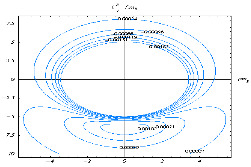
Figure 2: The plot shows the equicharge lines in the induced charge density for $v=0.55c$ with a fixed color charge $Q^{a}$ in the high temperature plasma.

In Fig. 2 we display the equicharge lines in the induced charge density for $v=0.55c$ in cylindrical coordinates which are scaled with $m_{g}=\sqrt{m_{D}^{2}/3}$. (The induced charge density is proportional to $m_{g}^{3}$.) The induced charge density is found to carry a screening charge cloud with a sign flip along the direction of the moving charge. As discussed in the preceding subsection II.3 there will be an excitation of modes during such a wake but they will be severely Landau damped through induced emission and absorption of the plasmons by scattering off single particles. As a result the particle suffers an energy loss through elastic collisions which can be described by (19) and has been studied extensively in the literature Thoma91 . When a charged particle moves with a velocity of less than $0.77c$, $\gamma v\leq 2.5$, the soft part of the collisional energy loss, caused by the induced chromoelectric field, turns out to be important Munshi ; Jane ; Moore05 ; Munshi05 .

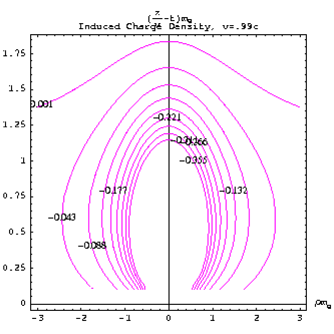
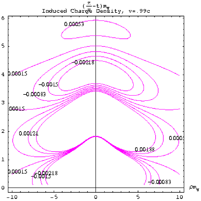
Figure 3: Left panel: The plot reproduces the equicharge lines in the induced charge density for $v=0.99c$ with a fixed color charge $Q^{a}$ in the high temperature plasma as obtained in Ref. Ruppert . Right panel: Same as left panel but plotted with more number of equicharge lines with enlarged axes to show the oscillations in the same density wake.

Next we consider the case when a charged particle moves faster than the average speed of the plasmon. For this purpose we choose $v=0.99c$ and the result is shown in the left panel of Fig. 3 which reproduces the corresponding results of Ref. Ruppert . The wake in the induced charge density apparently does not show any sign flip as in Fig. 2 and it shows merely a screening cloud around a test charge similar to that given in (36). However, this is not the case as the particular analysis in  Ruppert was not complete and some important features were obviously missing in the wake of the medium.

The complete analysis is shown in the right panel of Fig. 3 when the same data corresponding to the left panel are plotted with enlarged axes with a larger number of equicharge lines in the induced charge density. As expected the wake of the medium is clearly visible in the induced charge density which follows the charged particle traveling with a velocity, $v=0.99c$. Moreover, the screening cloud following the charge particle is found to flip its sign alternately indicating enhanced and depleted charge density. As discussed in the preceding subsection II.3 there will be an excitation in the plasmon modes during such a wake which could emit a Cerenkov like radiation with a Mach cone structure trailing the moving parton. The radiation is like a spontaneous emission of plasmon waves and cannot be calculated through the expression given in (19) and requires a special treatment. It is also important to note that for a parton velocity $v=0.99c$, $\gamma v\geq 4$, corresponding to the ultra-relativistic limit Moore05 ; Munshi05 for which the hard contribution of the collisional energy loss due to elastic scattering and the radiative energy loss are expected to be dominant.

When a parton moves supersonically, it excites waves in a colored plasma. The propagation of sound waves could be estimated from the emission pattern of secondary particles traveling at an angle with respect to the jet axis through the relation Stocker ; Ruppert

$$\Delta\phi=\pi\pm\phi_{M}\,=\pi\pm\arccos\left(\frac{c_{s}}{v}\right)\,,$$ (37)

where $\Delta\phi=\pi$ corresponds to the location of a maximum distribution of secondary hadrons from the away side jet in $p+p$ collisions, where no medium effects are present. However, due to medium effects the azimuthal angle for secondaries is expected to be peaked differently from $\pi$ and could be related to the Mach opening angle, $\phi_{M}$.

There are several programs in STAR and PHENIX experiments at RHIC where various approaches are being followed in order to find Mach cones. The basic approach is to use correlations between high $p_{\bot}$ secondary particles in pseudorapidity and azimuthal space. Some of the background correlation effects which might mimic Mach cones are being studied in details. Both the experiments are looking at 3-particle correlations which will eliminate the trivial backgrounds. Now already some interesting results have been reported by the PHENIX collaboration Azimuthal where the data suggest that the peak in the secondary particle correlation provides compelling evidence for a strong modification of the away-side jet. This could indicate two possible scenarios: (i) a Cerenkov jet in which the leading and away-side jet axes are aligned but fragmentation is confined to a very thin hollow cone or (ii) a directed jet in which the away-side jet axes are misaligned. A more quantitative investigation is necessary to distinguish between a $`$Cerenkov jet’ that leads to a Mach cone, $\phi_{M}$ and a $`$directed jet’ which is misaligned. Following (37) the azimuthal angle can be estimated here as $\Delta\phi\approx\pi\pm 1.01$ using $c_{s}=0.48$ within the HTL approximation. Once a characteristic correlation structure in secondary hadrons leading to a Mach cone, $\phi_{M}\sim 1.01$ is confirmed experimentally, it would provide an estimation of the angular structure of the energy loss and also the speed of sound in the QGP.

In Ref.Flow it was argued that the wake of an energetic parton can create an observable flow in the QGP. However, it was also argued that this is only the case if the energy loss of the parton is very large (about 12 Gev/fm). Even combining the collisional and radiative contributions, we do not expect such an high energy loss in relativistic heavy-ion collisions.

II.5 The Wake in the Screening Potential

Combining (14) and (16) the screening potential in configuration space due to the motion of a color charge can be written as Mustafa05

$$\Phi^{a}\left(\vec{\mathbf{r}},\vec{\mathbf{v}},t\right)=\frac{Q^{a}}{2\pi^{2}}\int d^{3}k\frac{e^{i\vec{\mathbf{k}}\cdot\left(\vec{\mathbf{r}}-\vec{\mathbf{v}}t\right)}}{k^{2}\epsilon_{L}\left(\omega=\vec{\mathbf{v}}\cdot\vec{\mathbf{k}},k\right)}\,.$$ (38)

In cylindrical coordinates, the screening potential in (38) becomes

$$\Phi^{a}\left(\rho,z,t\right) = \frac{2Q^{a}}{\pi v}\int_{0}^{\infty}d\kappa\,\kappa J_{0}\left(\kappa\rho\right)\int_{0}^{\infty}\,d\omega\frac{1}{k^{2}\Delta\left(\omega,k\right)}\left[\cos\left\{{\omega\left(\frac{z}{v}-t\right)}\right\}\,{\rm{Re}}\,\epsilon_{L}+\sin\left\{\omega\left(\frac{z}{v}-t\right)\right\}\,{\rm{Im}}\,\epsilon_{L}\right]\,.$$ (39)

where, $k=\sqrt{\kappa^{2}+{\omega^{2}}/{v^{2}}}$ and $\Delta=\left({\rm{Re}}\,\epsilon_{L}\right)^{2}+\left({\rm{Im}}\,\epsilon_{L}\right)^{2}$.

The potential in (38) is also solved for two special cases, (a) along the direction of motion of the parton $(\vec{r}\parallel\vec{v})$ and (b) perpendicular to the direction of motion of the parton $(\vec{r}\perp\vec{v})$. The potential for the parallel case is obtained as

$$\Phi^{a}_{\parallel}\left(\vec{r},\vec{v},t\right)=\frac{2Q^{a}}{\pi}\int_{0}^{\infty}dk\int_{0}^{1}\,dx\left[\cos\left(kx\left|\vec{\mathbf{r}}-\vec{\mathbf{v}}t\right|\right)\,\frac{{\rm{Re}}\ \epsilon_{L}}{\Delta}+\sin\left(kx\left|\vec{\mathbf{r}}-\vec{\mathbf{v}}t\right|\right)\,\frac{{\rm{Im}}\ \epsilon_{L}}{\Delta}\right]\ ,$$ (40)

whereas that for the perpendicular case is

$$\Phi^{a}_{\bot}\left(\vec{r},\vec{v},t\right) = \frac{Q^{a}}{2\pi^{2}}\int_{0}^{\infty}dk\int_{0}^{2\pi}\,d\phi\int_{-1}^{1}dx\frac{e^{ik\left[r\cos{\phi}\sqrt{1-x^{2}}-vxt\right]}}{\epsilon_{L}\left(\omega=vkx,k\right)}$$ (41)

$$= \frac{2Q^{a}}{\pi}\int_{0}^{\infty}dk\int_{0}^{1}dx\frac{J_{0}\left(kr\sqrt{1-x^{2}}\right)}{\Delta}\left[\cos{(kvxt)}\,{\rm{Re}}\ \epsilon_{L}-\sin{(kvxt)}\,{\rm{Im}}\ \epsilon_{L}\right]\,,$$

with $x=\cos\theta$. We point out here that some efforts were made earlier in studying the wake potential Chu89 ; Mustafa05 in a QGP. However, those were incomplete, neglecting Mach cones and Cerenkov radiation in the wake of the plasma due to the motion of the charged particle.

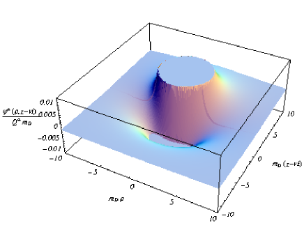
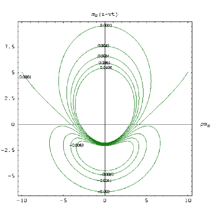
Figure 4: Left panel: Spatial distribution of the scaled wake potential with respect to $m_{D}$ from a jet with a fixed color charge $Q^{a}$ which is traveling with $v=0.55c$. Right panel: This plot shows the corresponding equipotential lines.

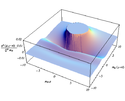
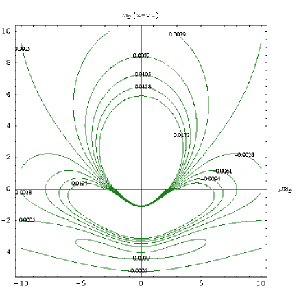
Figure 5: Same as Fig. 4 but $v=0.99c$.

In Fig. 4 the wake potential is plotted for $v=0.55c$ in cylindrical coordinates which is scaled with $m_{D}$. (The wake potential is proportional to $m_{D}$.) The left panel shows a three dimensional plot of the wake potential whereas the right panel displays the corresponding equipotential lines. It should be noted that the potential depends only on $v$ and not on $t$ as it should be for an isotropic and homogeneous plasma. The spatial distribution of the potential shows the well known singular behavior at $r=0$, i.e. $z=0$ and $\rho=0$, which has been cut by hand through the scale restriction in the left panel. It also exhibits a well defined negative minimum in the $(\rho-z)$ plane which has been formed due to the dynamical screening in the vicinity of the moving charged particle. This feature is also obvious in the right panel where the equipotential lines are found to flip their sign in the ($\rho-z$) plane corresponding to a moving induced charge cloud of opposite sign as shown in Fig. 2, forming the wake around a moving particle.

When the velocity of the charged particle is higher than the average plasmon speed ($0.77c$), the induced charged cloud trailing the charged particle begins to oscillate which in turn indicates an oscillatory wake potential and has not been found in earlier studies Chu89 ; Mustafa05 . In Fig. 5 we display the spatial distribution of the wake potential for $v=0.99c$ which shows oscillations in the $(\rho-z$) plane. Such oscillations, as discussed in the preceding sub-sections, lead to an emission of Cerenkov like radiation and generate Mach shock waves. This is analogous to the wake phenomena in classical plasmas in the supersonic regime Bashkirov04 .

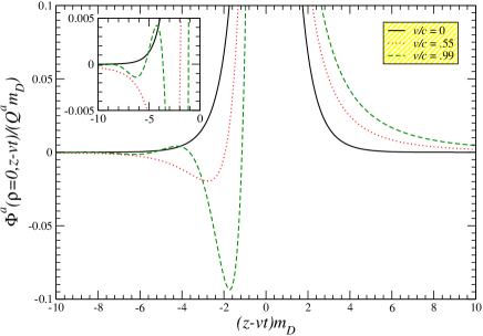
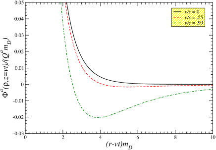
Figure 6: Left panel: Scaled screening potential along the $z$-axis, i.e., parallel to the direction of the moving color charge $Q^{a}$ for different velocities. Right panel: Same as left panel but along the $\rho$-axis, i.e., perpendicular to the direction of the color charge.

In Fig. 6 the wake potentials in the specific directions corresponding to Figs. 4 and 5 are displayed. The left panel shows a wake potential along the $z$-axis, i.e., parallel to the direction of the moving color charge. This could be directly obtained from (40) or by setting $\rho=0$ in (39). As expected the singular behavior at $z=0$ is clearly reflected in this plot. In the outward flow, i.e., in the negative $z$-direction the wake potential compared to the static one (i.e., for $v=0$) falls off very fast, reverses its sign, exhibits a negative minimum and asymptotically approaches zero from below. For $v\leq 0.77c$ the potential in the outward flow is found to be of the Lennard-Jones type Kittel which has a short range repulsive part as well as a long range attractive part. With increase of $v$ the depth of the negative minimum increases and its position shifts towards the origin or to the particle. When $0.77c<v<c$, the wake potential begins to oscillate. For $v=0.99c$ such oscillations in the wake potential along the direction of the motion are also clearly visible in the outward flow ($z<0$) from the inset of the left panel in Fig. 6. On the other hand the potential for incoming flow, i.e., in the positive $z$-direction does not show any such structure and behaves more like a modified Coulomb potential. However, with the increase of $v$ it attains a Coulombic form indicating that the forward part of the screening cloud is not so strongly affected by the motion of the particle.

Figs. 4, 5 and 6 reveal that at finite $v$ the potential in the $z$-direction becomes anisotropic and loses forward-backward symmetry with respect to the motion of the charged particle. The origin of this can be traced back to the second term in (39) and/or (40) which is antisymmetric under inversion of $(z-vt)\rightarrow-(z-vt)$. This term appears due to the antisymmetric nature of the imaginary part of $\epsilon_{L}(k,\omega)$ in (34). So, the effect of finite $v$ is not limited only to the deformation of the screening cloud, but, more importantly, it shifts the position of the test charge off the centre of the wake potential. As a consequence, the test charge experiences a retarding force from the plasma. This leads to a stopping power of the QGP against a moving test charge. The nature of the energy loss leading to such stopping power of the QGP has already been discussed in the preceding subsec. II.4. We also note that a minimum in the screening potential for a moving color charge was found in earlier works by Chu and Matsui Chu89 and also by us Mustafa05 in the direction of propagation. However, in Ref. Chu89 Chu and Matsui did not report this minimum whereas our earlier study Mustafa05 was incomplete concerning the forward-backward asymmetry of the wake structure and Cerenkov radiation.

On the other hand, the right panel of Fig. 6 displays the wake potential normal to the direction of motion of the charged particle. This could be obtained directly from (41) or by setting $z=0$ in (39) which shows the usual singularity at $\rho=0$ and a symmetric behavior in $\rho$. It also falls off very fast compared to the static case and the nature of the potential is found to be of the Lennard-Jones type due to the deformed screening cloud forming the wake in the vicinity of the moving charged particle. With increase of $v$, the position of the minimum shifts towards the origin and the depth of it increases. Such kind of potential in the normal direction implies that a part of the screening cloud forming the wake due to the motion of the charged particle along the $z$-direction is also moving away in the perpendicular direction, resulting in a transverse flow in the medium. This behavior was not observed in earlier studies Chu89 ; Mustafa05 .

The negative minimum in the wake potential indicates an induced space charge density of opposite sign. Thus, a particle moving relative to a particle in the induced space charge density would constitute a dipole oriented along the direction of motion. In the next sub-section, we calculate the potential due to such dipole interaction in the QGP.

II.6 Dipole Potential in the QGP

We consider two color charges $Q^{a}$ and $Q^{b}$ separated by a distance $r$. The change in free energy of the system to bring the two widely separated color charges together Lebellac ; Blaizot ; Zee is

$$\Delta{\mathcal{F}} = \frac{1}{2}\int d^{3}{\vec{\mathbf{x}}}\,J^{\mu}_{\rm{ext}}\left(x\right)A_{\mu}\left(x\right)=\frac{1}{2}\int\frac{d^{3}k}{\left(2\pi\right)^{3}}\int_{-\infty}^{\infty}\frac{d\omega}{\left(2\pi\right)}\int_{-\infty}^{\infty}\frac{d\omega^{\prime}}{\left(2\pi\right)}e^{it\left(\omega+\omega^{\prime}\right)}J^{\mu}_{\rm{ext}}\left(\omega,-\vec{\mathbf{k}}\right)A_{\mu}\left(\omega^{\prime},\vec{\mathbf{k}}\right)\,,$$ (42)

where $J^{\mu}_{\rm{ext}}\left(x\right)=\left(\rho_{\rm{ext}},\vec{\mathbf{J}}_{\rm{ext}}\right)$ is the sum of the two external currents, $J^{\mu}_{\rm{ext}}\left(x\right)=J^{\mu}_{1}\left(x\right)+J^{\mu}_{2}\left(x\right)$, and $A_{\mu}\left({\vec{\mathbf{x}}}\right)$ is the associated gauge field. The entropy generation is neglected in (42).

We assume that the average value of $A_{\mu}$ vanishes in equilibrium $\left\langle A_{\mu}\right\rangle_{\mbox{eq}}=0$. The induced expectation value of the vector potential, $A_{\mu}$ follows from linear response theory Weldon82 as

$$\langle A_{\mu}\rangle_{\beta}=4\pi\Delta_{\mu\nu}\left(\Omega,{\vec{\mathbf{k}}}\right)\,J^{\nu}_{\rm{ext}}(K)\ \ ,$$ (43)

where, $\Omega=u.K,\ k=\sqrt{\Omega^{2}-K^{2}}$ are the Lorentz invariant energy and 3-momentum, respectively. $\Delta_{\mu\nu}$ is the propagator of the gauge boson exchanged between the two currents which is given in (26). Combining (43) with (42) we can write

$$\Delta{\mathcal{F}} = 2\pi\int\frac{d^{3}k}{\left(2\pi\right)^{3}}\int_{-\infty}^{\infty}\frac{d\omega}{\left(2\pi\right)}\int_{-\infty}^{\infty}\frac{d\omega^{\prime}}{\left(2\pi\right)}e^{it\left(\omega+\omega^{\prime}\right)}J^{\mu}_{\rm{ext}}\left(\omega,-\vec{\mathbf{k}}\right)\Delta_{\mu\nu}(\omega^{\prime},{\vec{\mathbf{k}}})J^{\nu}_{\rm{ext}}(\omega^{\prime},{\vec{\mathbf{k}}})\,.$$ (44)

One can obtain the dipole interaction in (44) by separating Weldon82 the current, in general, into a charge density that moves with the fluid velocity $u^{\mu}$ and a spacelike current flow either longitudinal or transverse to ${\tilde{K}}^{\mu}$ as defined in (23):

$$J^{\mu}(K)=u^{\mu}u^{\alpha}J_{\alpha}(K)+J^{\mu}_{L}(K)+J^{\mu}_{T}(K)\ \ ,$$ (45)

where

$$J^{\mu}_{L}(K) = \frac{\tilde{K}^{\mu}\omega}{k^{2}}u^{\alpha}J_{\alpha}(K)\,,$$

$$J^{\mu}_{T}(K) = \left[\tilde{\eta}^{\mu}_{\lambda}+\frac{\tilde{K}^{\mu}\tilde{K}_{\lambda}}{k^{2}}\right]J^{\lambda}(K)\,.$$ (46)

Using (26) and (45) the dipole interaction can be obtained as

$$J^{\mu}\left(\omega,-\vec{\mathbf{k}}\right)\Delta_{\mu\nu}(\omega^{\prime},{\vec{\mathbf{k}}})J^{\nu}(\omega^{\prime},{\vec{\mathbf{k}}}) = -\frac{k^{2}+\omega\omega^{\prime}}{\omega\omega^{\prime}}\frac{\vec{\mathbf{J}}_{L}(\omega,-\vec{\mathbf{k}}){\mathbf{\cdot}}\vec{\mathbf{J}}_{L}(\omega,\vec{\mathbf{k}})}{{\omega^{\prime}}^{2}-k^{2}-\Pi_{L}(\omega^{\prime},k)}-\frac{\vec{\mathbf{J}}_{T}(\omega,-\vec{\mathbf{k}}){\mathbf{\cdot}}\vec{\mathbf{J}}_{T}(\omega,\vec{\mathbf{k}})}{{\omega^{\prime}}^{2}-k^{2}-\Pi_{T}(\omega^{\prime},k)}$$ (47)

$$= \frac{\vec{\mathbf{J}}(\omega,-\vec{\mathbf{k}}){\mathbf{\cdot}}\vec{\mathbf{J}}(\omega,\vec{\mathbf{k}})+\frac{\omega\omega^{\prime}}{k^{2}}{\rho(\omega,-\vec{\mathbf{k}})\rho(\omega,\vec{\mathbf{k}})}}{{\omega^{\prime}}^{2}-k^{2}-\Pi_{T}(\omega^{\prime},k)}\,\,$$

$$-\frac{k^{2}+\omega\omega^{\prime}}{k^{2}}\frac{\rho(\omega,-\vec{\mathbf{k}})\rho(\omega,\vec{\mathbf{k}})}{{\omega^{\prime}}^{2}-k^{2}-\Pi_{L}(\omega^{\prime},k)}\,\,,$$

where $u.J=\rho$. Though the gluon propagator in (26) is gauge dependent, the dipole interaction becomes gauge independent.

We begin with the known example of screening of two static charges $Q^{a}$ and $Q^{b}$ at position $\vec{\mathbf{x}}_{1}$ and $\vec{\mathbf{x}}_{2}$, respectively. The corresponding dipole current is given by

$$J^{\mu}\left(x\right)=J^{\mu}_{1}\left(x\right)+J^{\mu}_{2}\left(x\right)=\delta^{\mu}_{0}\left[Q^{a}\delta\left(\vec{\mathbf{x}}-\vec{\mathbf{x}}_{1}\right)+Q^{b}\delta\left(\vec{\mathbf{x}}-\vec{\mathbf{x}}_{2}\right)\right]\stackrel{{\scriptstyle\mbox{FT}}}{{=}}2\pi\delta_{0}^{\mu}\delta\left(\omega\right)\left[Q^{a}e^{-i\vec{\mathbf{k}}\cdot\vec{\mathbf{x}}_{1}}+Q^{b}e^{-i\vec{\mathbf{k}}\cdot\vec{\mathbf{x}}_{2}}\right]\,.$$ (48)

Combining (48), (47) and (44), and also dropping the self coupling terms we get the well known Yukawa potential as

$$\Delta{\mathcal{F}}^{ab}(r)=\frac{Q^{a}Q^{b}}{2\pi^{2}}\int d^{3}k\,\frac{\cos\left({\vec{\mathbf{k}}}\cdot{\vec{\mathbf{r}}}\right)}{\kappa^{2}+k^{2}_{z}+m_{D}^{2}}=Q^{a}Q^{b}\,\frac{e^{-m_{D}r}}{r}\,,$$ (49)

where, $\vec{\mathbf{r}}={\vec{\mathbf{x}_{1}}}-{\vec{\mathbf{x}_{2}}}$ and ${\vec{\mathbf{r}}}=\left(\rho,0,z\right)$. It is also noteworthy to mention that in Ref. Gale87 a static screening potential was also obtained in a QGP, where a polarization tensor beyond the high temperature limit was used. However, this approach in Ref. Gale87 has its limitation because a gauge dependent and incomplete approximation for the polarization tensor was used.

Now for two comoving charges $Q^{a}$ and $Q^{b}$ the dipole current can be written as

$$J_{\mu}\left(t,{\vec{\mathbf{x}}}\right)=\left(1,{\vec{\mathbf{v}}}\right)\left[Q^{a}\delta\left({\vec{\mathbf{x}}}-{\vec{\mathbf{x}}_{1}}-{\vec{\mathbf{v}}}t\right)+Q^{b}\delta\left({\vec{\mathbf{x}}}-{\vec{\mathbf{x}}_{2}}-{\vec{\mathbf{v}}}t\right)\right]\stackrel{{\scriptstyle\mbox{FT}}}{{=}}2\pi\left(1,{\vec{\mathbf{v}}}\right)\delta\left(\omega-{\vec{\mathbf{k}}}\cdot{\vec{\mathbf{v}}}\right)\left[Q^{a}e^{-i{\vec{\mathbf{k}}}\cdot{\vec{\mathbf{x}}_{1}}}+Q^{b}e^{-i{\vec{\mathbf{k}}}\cdot{\vec{\mathbf{x}}_{2}}}\right]\,,$$ (50)

and we obtain the dipole potential as

$$\Delta{\mathcal{F}}^{ab}(r;\rho,z) = \frac{Q^{a}Q^{b}}{2\pi^{2}}\int d^{3}k\,\cos\left({{\vec{\mathbf{k}}}\cdot{\vec{\mathbf{r}}}}\right)\left[\frac{v^{2}-\frac{\omega^{2}}{k^{2}}}{K^{2}-\Pi_{T}\left(\omega,k\right)}-\frac{1-\frac{\omega^{2}}{k^{2}}}{K^{2}-\Pi_{L}\left(\omega,k\right)}\right]_{\omega={\vec{\mathbf{k}}}\cdot{\vec{\mathbf{v}}}}\,,$$ (51)

$$= \frac{2Q^{a}Q^{b}}{\pi}\int_{0}^{\infty}d\kappa\,\kappa J_{0}\left(\kappa\rho\right)\int_{0}^{\infty}dk_{z}\,\cos\left({k_{z}z}\right)\,\,\left\{{\rm{Re}}\,\left[\frac{v^{2}-\frac{\omega}{k^{2}}}{K^{2}-\Pi_{T}\left(\omega,k\right)}-\frac{1-\frac{\omega^{2}}{k^{2}}}{K^{2}-\Pi_{L}\left(\omega,k\right)}\right]_{\omega={\vec{\mathbf{k}}}\cdot{\vec{\mathbf{v}}}}\right\}.$$

The following features are transparent in (51). The first term corresponds to the transverse (magnetic) interaction whereas the second term is due to the longitudinal (electric) interaction. Like the single body potential in (39) the two body potential is also symmetric in $\rho$. Moreover, in (51) both imaginary parts corresponding to the longitudinal and transverse response functions drop out because they are odd in $k_{z}$, which make both terms symmetric under the inversion of $z\ \rightarrow\ -z$, thus the total potential. This is, however, unlike the single body potential in (39) where the presence of an imaginary part of the longitudinal response function was found to be responsible for the asymmetric behavior. In addition the two body potential should be symmetric in $z$ as the two color charges are moving opposite to each other which is obvious from the dipole interaction in (47). Recalling Ampere’s law this would also amount to an attraction between color charges traveling opposite to each other along the $z$ axis. Both the electric and magnetic interactions play a crucial role, as we will see below.

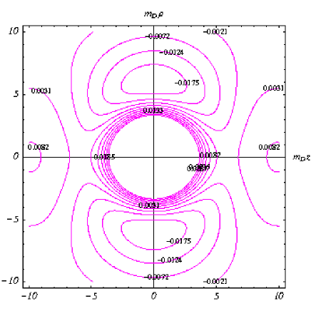
Figure 7: Left panel: Spatial distribution of the longitudinal part of the scaled dipole potential with respect to $m_{D}$ in which the two color charges are traveling antiparallel to each other with $v=0.55c$. Right panel: This plot shows the corresponding equipotential lines.

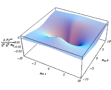
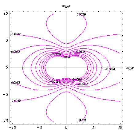
Figure 8: Same as Fig. 7 but showing the transverse part.

In Fig. 7 the spatial distribution of the scaled  longitudinal part of the two body potential in cylindrical coordinate is displayed for $v=0.55c$. The left panel shows a three dimensional plot of it whereas the right panel displays the corresponding equipotential lines. The longitudinal part has a singularity at $r=0$, i.e., $z=0$ and $\rho=0$, clearly reflected in Fig. 7. As discussed above the potential plotted in both panels is found to be completely symmetric in the ($\rho-z$) plane along with a variable minimum. Such a minimum in the $(\rho-z$) plane is due to the fact that the electric interaction contributes differently in $z$ as well as in $\rho$ direction. The potential has a positive minimum in the longitudinal direction, i.e., along the $z$ axis and then tends to zero for large $|z|$. This can also be seen from the left panel of Fig. 10, which can be obtained from (51) by setting $\rho=0$. On the other hand, in the transverse direction, i.e., along the $\rho$ direction, the electric contribution has a well defined negative minimum, it also attains a positive maximum at large $\rho$ and slowly approaches zero asymptotically. This feature can clearly be seen from the right panel of Fig. 10, which is obtained by solving (51) with $z=0$.

The contribution of the scaled transverse part is shown in Fig. 8 which is also found to be symmetrical in the $(\rho-z)$ plane along with a well defined negative minimum. However, both panels indicate that the magnetic interaction contributes differently in $z$ as well in $\rho$ directions, which can also be seen from Fig. 10. In the limit $v\rightarrow 0$, the transverse part vanishes. However, for any nonzero value of $v$ the transverse part begins with a finite negative value for both cases. As $|z|$ increases, its magnitude gradually decreases and approaches zero for large $|z|$ (left panel of Fig. 10) whereas in the transverse direction its magnitude decreases faster, becomes positive at certain values of $\rho$, and then slowly approaches zero for large values of $\rho$ (right panel of Fig. 10).

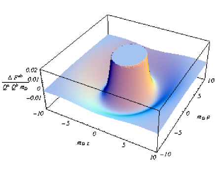
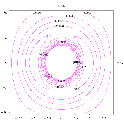
Figure 9: Total contribution for $v=0.55c$

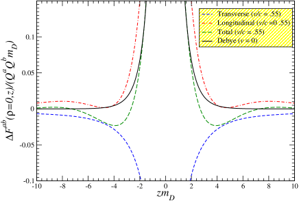
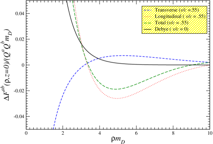
Figure 10: Left panel: Scaled two body potential along the direction of motion when two color charges are traveling antiparallel to each other with $v=0.55c$. Right panel: Same as left panel but normal to the direction of motion.

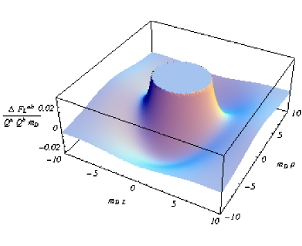
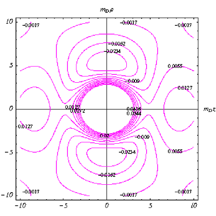
Figure 11: Left panel: Spatial distribution of the longitudinal part of the scaled dipole potential with respect to $m_{D}$ in which two color charges are traveling antiparallel to each other with $v=0.99c$. Right panel: This plot shows the corresponding equipotential lines.

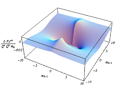
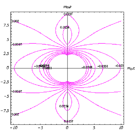
Figure 12: Same as Fig. 11 but showing the transverse part.

The spatial distribution of the total potential for $v=0.55c$ is displayed in Fig. 9, which appears due to the compensating effects between the electric and the magnetic interactions as discussed above. The resulting potential shows the usual singularity of the screening potential at $r=0$ ($z=0$ and $\rho=0$) and a completely symmetric behavior along with a pronounced negative minimum in the $(\rho-z)$ plane, which are clearly reflected in both panels of Fig. 9. However, the detailed features in the specific direction can also be seen from both panels of Fig. 10. The potential along the $|z|$-direction as shown in the left panel falls off like that of a static one, flips its sign, exhibits a negative minimum, and then oscillates around zero. As can be seen from the left panel, the competing effects between electric and magnetic contributions with opposite sign result in an oscillatory potential along the $z$ direction. On the other hand, the potential in the transverse direction (right panel) falls off slowly compared to the static one, flips its sign, and exhibits a negative minimum at some values of $\rho$, again changes its sign to attain small positive maximum and then tends to zero at large $\rho$. It can be seen that the nature of the potential is completely dictated by the electric interaction rather than by the magnetic one. In both directions there are oscillations at large distances but the form of the potential mostly resembles the Lennard-Jones type with a pronounced repulsive as well attractive part.

With the increase of $v$, as we will see below, the relative strength of the dipole potential grows strongly. For $v=0.99c$ Fig. 11 displays the spatial distribution of the scaled longitudinal potential whereas Fig. 12 shows that of transverse part in the ($\rho-z$) plane. These plots clearly show that the magnitude of the spatial distribution of the dipole potential due to both electric and magnetic interactions are enhanced to a large extent in the ($\rho-z$) plane. The resulting potential distribution is shown in Fig. 13. Apart from the usual features as discussed above for smaller $v$, it displays a new and important feature. A substantial repulsive interaction has grown in the transverse plane, i.e., in the direction of $\rho$ but at $z=0$, becoming responsible for a vertical split of the minimum in the $(\rho-z)$ plane as can be seen from both the panels in Fig. 13.

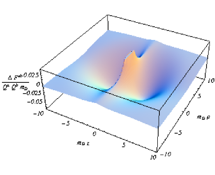
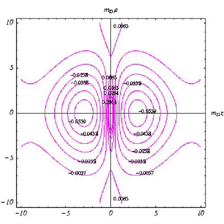
Figure 13: Total contribution for $v=0.99c$

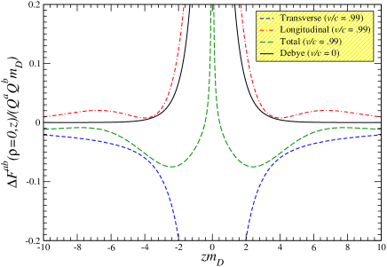
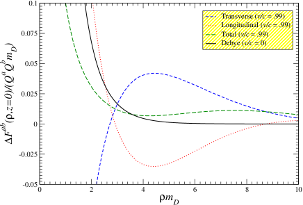
Figure 14: Same as Fig. 10 but $v=0.99c$.

Now, the detailed contributions of both the interactions can also be understood from both panels of Fig. 14 where the dipole potentials for two special cases have been displayed. As shown in the left panel of Fig. 14 the depth of the negative minimum of the dipole potential along the $|z|$ direction increases and it position shifts towards the centre indicating a faster fall off as well as a larger anisotropy. This is due to the fact that the magnitude of the magnetic interaction becomes dominant. The form of the potential remains of the Lennard-Jones type. On the other hand, the potential in the transverse direction ($z=0$) as shown in the right panel of Fig. 14 is oscillatory as well as repulsive, which is again due to the dominant magnetic interaction in the transverse direction. So, with the increase of $v$ the magnetic interaction due to the transverse part of the response function plays a crucial role and its form deviates from the Lennard-Jones type. This could have important consequences on various binary states in the QGP.

In QCD the interaction between color charges in various channels is either attractive or repulsive. A quark and an antiquark correspond to the sum of irreducible color representations : $\mathbf{3\otimes{\bar{3}}={\bar{1}}\oplus 8}$, where the interaction strength of the color singlet representation is $-16/3$ (attractive) whereas that of the color octet channel is $2/3$ (repulsive). Similarly, a two quark state corresponds to the sum of the irreducible color representations: $\mathbf{3\otimes 3={\bar{3}}\oplus 6}$, where the antisymmetric color triplet is attractive ($-8/3$) giving rise to possible bound states Shuryak . The symmetric color sextet channel, on the other hand, is repulsive ($4/3$). Color bound states (i.e. diquarks) of partons at rest have been claimed by analyzing lattice data Shuryak . The situation is different when partons are in motion. The dipole potentials along the direction of propagation and also normal to it have both attractive and repulsive parts, similar to the Lennard-Jones form. So, all the attractive channels or the repulsive channels in the static case get inverted due to the two comoving partons constituting a dipole in the QGP. This could lead to dissociation of bound states (or to resonance states) as well formation of color bound states in the QGP.

Recent lattice results Datta using maximum entropy method indicate that charmonium states actually persist up to $2T_{C}$ and there are similar evidence for mesonic bound states made of light quarks as well Karsch . Within our model such bound states as well other colored binary states in the QGP can experience different potentials along the dipole direction and the direction normal to it. Along the direction of motion binary states which were bound in the QGP may become resonance states or dissociate beyond $T_{C}$. The temperature up to which they survive need further analysis of the bound states properties in detail, which is beyond the scope of this work. Similarly, those colored states which were not bound initially in the QGP, may transform into bound states. There are some long distance correlations among partons in the QGP, which could indicate the appearance/disappearance of binary states in the QGP beyond $T_{C}$. On the other hand, in the transverse direction the mesonic states as well as colored bound binary states may dissociate for smaller velocity of comoving partons whereas they may remain loosely bound if the comoving partons are ultra-relativistic. One immediate consequence of this would be the modification of the transverse momentum, $p_{\bot}$, dependence of $J/\psi$ spectra. Our analysis suggests that a QGP with moving partons beyond $T_{C}$ does not behave as a free gas of partons but a long range correlation may be present.

III Conclusions

We have investigated the response of the QGP to a fast moving parton within the HTL approximation valid in the high temperature limit. For velocities smaller than the phase velocity of the longitudinal plasma mode $v=\sqrt{3/5}c$ the wake potential corresponds to dynamical, anisotropic screening as discussed already before Mustafa05 . For larger velocities, however, we found, in contrast to previous investigations Mustafa05 ; Ruppert that Mach cones and Cerenkov radiation appear in addition. They have been identified by oscillations (sign flips) in the induced charge density and also in the wake potential in the outward flow. This observation could be of phenomenological interest for the present experimental programs in RHIC, where various approaches are being followed to find Mach cones through the correlation between high $p_{\bot}$ secondary particles in pseudorapidity and azimuthal space. The general structure of the wake potential in the direction of motion shows a long range correlation among the particles in colored plasma. The consequences for the formation of a possible liquid phase of the QGP Thoma_2005 should be investigated. In addition, the wake potential normal to the motion of the charged particle causes a transverse flow in the system which might contribute to the creation of instabilities Mrow and an anomalous viscosity Asakawa .

Furthermore, we have investigated the dipole potential by comoving (anti)quarks in the QGP due to the appearance of a minimum in the wake potential of a moving color charge, extending the work in Ref.Mustafa05 . In Ref. Mustafa05 the dipole potential was obtained by averaging the one body potential and the dipole potential was found to be dependent only on the electric interaction. In the present work we followed a proper treatment, as depicted in subsec. II.6, and the dipole potential was found to depend on both electric and magnetic interactions. As discussed both interactions play a crucial role in determining the nature of the dipole potential. Based on this we analyzed the various possibilities, viz., the appearance/disappearance of bound states in the QGP by discussing the effects of Ampere’s law and the nature of electric and magnetic forces due to dynamical screening.

References

- (1) S. Ichimaru, Basic Principles of Plasma Physics (Benjamin, Reading, 1973).
- (2) L.P. Pitaevskii and E.M. Lifshitz, Physical Kinetics (Pergamon Press, Oxford, 1981).
- (3) E. V. Shuryak, Sov. Phys. JETP 47, 212 (1978).
- (4) B. Müller, The Physics of the Quark-Gluon Plasma, Lecturer Notes in Physics 225 (Springer-Verlag, Berlin, 1985).
- (5) J.I. Kapusta, Finite-Temperature Field Theory (Cambridge University Press, Cambridge, 1989).
- (6) M. LeBellac, Thermal Field Theory (Cambridge University Press, Cambridge, 2000).
- (7) K. Kajantie and J.I. Kapusta, Ann. Phys. (N.Y.) 160, 477 (1985).
- (8) S. Datta, F. Karsch, P. Petreczky and I. Wetzorke, Phys. Rev. D 69, 094507 (2004).
- (9) F. Karsch, E. Laermann, P. Petreczky, S. Stickan and I. Wetzorke, Phys. Lett. B 530,147 (2002); F. Karsch, Nucl. Phys. A 715, 701 (2003).
- (10) S. S. Adler et al. [PHENIX Collaboration], Phys. Rev. C 69, 034909 (2004).
- (11) K. Adcox et al. [PHENIX Collaboration], Phys. Rev. Lett. 89, 212301 (2002); S. S. Adler et. al.[PHENIX Collaboration], Phys. Rev. Lett. 91, 182301 (2003).
- (12) S. S. Adler et. al.[PHENIX Collaboration], Phys. Rev. Lett. 91, 072301 (2003).
- (13) K. Adcox et al. [PHENIX Collaboration], Phys. Rev. Lett. 88, 022301 (2002); C. Adler et al. [STAR Collaboration], Phys. Rev. Lett. 89 (2002) 202301; ibid 90, 032301 (2003); ibid 90, 082302 (2003); B.B. Back et al. [PHOBOS Collaboration], Phys. Lett. B 578, 297 (2004).
- (14) M. Gyulassy and M. Plümer, Phys. Lett. B 243, 432 (1990).
- (15) D. Teaney, J. Lauret, and E. V. Shuryak, Phys. Rev Lett. 86, 4783 (2001); P. F. Kolb, P. Huovinen, U. Heinz, and H. Heiselberg, Phys. Lett. B 500, 232 (2001); A. K. Chaudhuri, nucl-th/0604014.
- (16) M. Gyulassy, P. Levai, and I. Vitev, Phys. Lett. B 538, 282 (2002); M. Gyulassy, I. Vitev, X. N. Wang, Phys. Rev. Lett. 86, 2537 (2001).
- (17) B.G. Zakharov, JETP Lett. 63, 952 (1996);70, 176 (1999); 73, 49 (2001); C. A. Salgado and U. A. Wiedemann, Phys. Rev. Lett. 89, 092303 (2002).
- (18) E. Wang and X. N. Wang, Phys. Rev. Lett. 89, 162301 (2002).
- (19) R. Baier, Y. L. Dokshitzer, A. H. Mueller, and D. Schiff, JHEP 0109, 033 (2001).
- (20) B. Müller, Phys. Rev. C 67, 061901(R) (2003).
- (21) M. G. Mustafa and M. H. Thoma; Acta Phys. Hung. A 22, 93 (2005).
- (22) J. Alam, P. Roy and A. K. Dutt-Mazumder, hep-ph/0604131; A. K. Dutt-Mazumder, J. Alam, P. Roy, and B. Sinha, Phys. Rev. D 71, 094016 (2005).
- (23) J. Ruppert and B. Müller, Phys. Lett. B618, 123 (2005); B. Müller and J. Ruppert, nucl-th/0507043; J. Ruppert, J. Phys. Conf. Ser. 27, 217 (2005).
- (24) M. G. Mustafa, M. H. Thoma and P. Chakraborty, Phys. Rev. C 71, 017901 (2005).
- (25) M. H. Thoma and M. Gyulassy, Nucl. Phys. B351, 491 (1991).
- (26) A. Weldon, Phys. Rev. D26, 1394 (1982).
- (27) T. H. Elze and U. Heinz, Phys. Rep. 183, 81 (1989).
- (28) S. Mrówczyński, Quark-Gluon Plasma, Ed. R. Hwa (World Scientific, Singapore) p 185.
- (29) A. Das, Finite Temperature Field Theory (World Scientific, Singapore, 1997).
- (30) V. V. Klimov, Sov. Phys. JETP 55, 199 (1982).
- (31) M. H. Thoma, Quark Gluon Plasma 2, Ed. R. C. Hwa (World Scientific, Singapore, 1995) p. 51 .
- (32) E. Braaten and R. Pisarski, Nucl. Phys. B 337, 569 (1990).
- (33) U. Heinz, K. Kajantie, and T. Toimela, Ann. Phys. (N.Y.) 176, 218 (1987).
- (34) G. D. Moore and D. Teaney, Phys. Rev. C 71, 064904 (2005); H. van Hees and R. Rapp, Phys. Rev. C 71, 034907 (2005); H. van Hees, V. Greco and R. Rapp, Phys. Rev. C 73, 034913 (2006).
- (35) M. G. Mustafa, Phys. Rev C 72, 014905 (2005).
- (36) H. Stöcker, Nucl. Phys. A750, 121 (2005).
- (37) N. N. Ajitanand for PHENIX collaboration, nucl-ex/0511029; Nucl. Phys. A 774, 585 (2006).
- (38) J. Casalderrey-Solana, E.V. Shuryak, and D. Teaney, hep-ph/0602183.
- (39) M.-C. Chu and T. Matsui, Phys. Rev. D 39, 1892 (1989).
- (40) A. G. Bashkirov, Phys. Rev. E 69, 046410 (2004).
- (41) C. Kittel, Introduction to Solid State Physics (Wiley Eastern Limited, New Delhi, 1984).
- (42) C. Gale and J. Kapusta, Phys. Lett. B 198, 89 (1987).
- (43) J.-P. Blaizot, J.-Y. Ollitrault and E. Iancu, Quark-Gluon Plasma-2, Ed. R. C. Hwa (World Scientific, Singapore).
- (44) A. Zee, Quantum Field Theory in a nutshell (Princeton University Press, 2003).
- (45) E. V. Shuryak and I. Zahed, Phys. Rev. D 70, 054507 (2004).
- (46) M.H. Thoma, J. Phys. G 31, L7 (2005); Erratum, J. Phys. G 31 539 (2005).
- (47) S. Mrowcynski, Acta Phys. Pol B 37, 427 (2006)
- (48) M. Asakawa, S. A. Bass and B. Müller, Phys. Rev. Lett. 96, 252301 (2006).