Regge-cascade hadronization

Abstract

We argue that the evolution of coloured partons into colour-singlet hadrons has approximate factorization into an extended parton-shower phase and a colour-singlet resonance–pole phase. The amplitude for the conversion of colour connected partons into hadrons necessarily resembles Regge-pole amplitudes since $q\bar{q}$ resonance amplitudes and Regge-pole amplitudes are related by duality. A ‘Regge-cascade’ factorization property of the $N$-point Veneziano amplitude provides further justification of this protocol. This latter factorization property, in turn, allows the construction of general multi-hadron amplitudes in amplitude-squared factorized form from $(1\to 2)$ link amplitudes. We suggest an algorithm with cascade-decay configuration, ordered in the transverse momentum, suitable for Monte-Carlo simulation. We make a simple implementation of this procedure in Herwig++, obtaining some improvement to the description of the event-shape distributions at LEP.

1 Introduction

By ‘hadronization’, we loosely mean the final phase in the process of jet formation, where coloured partons at the end of the parton shower turn into colour-singlet hadrons.

The hadronization phase is presumably not completely separable from the perturbative phase, but approximations can be made, and we can for instance set the perturbative coupling to zero in the hadronization phase and vice versa. This is, in effect, the approach ordinarily taken in the Monte-Carlo event generators herwig ; pythia .

A better approximation may be to allow the perturbative coupling to extend into the hadronization phase, and continue the perturbative evolution down to zero odagirihadronization .

The universality, i.e., that it does not depend on, for instance, where the other partons are, of the cut-off in the first case and the coupling in the second case can be justified in the Gribov confinement picture gribov . Although the complete treatment of the gluon Green’s function is lacking at present, for the quark Green’s function, Gribov’s method indicates that its behaviour is governed by a universal equation containing both the gluonic semi-perturbative and the long-distance super-critical contributions. We can then separate out the semi-perturbative contribution by means of the effective coupling procedure, so that the remaining dynamics, of hadronization, would be a predominantly colour-singlet interaction, mediated by resonances and poles. In other words, the coloured partons that remain at the end of the extended parton-shower phase turn into hadrons by an interaction which is effectively colour-singlet.

Colour preconfinement amati_veneziano ; preconfinement dictates that at the end of the parton shower, the colour-connected parton pairs, i.e., the colour dipoles, have a mass spectrum with a characteristic scale of a few times the parton-shower cut-off, and this mass scale normally comes out to be about 1 GeV. However, this is violated in low-$p_{T}$ jets odagirisue .

As is the case in the Monte Carlo event generators, let us consider these colour-preconfined units as the starting point of hadronization. The colour-connected partons then exchange objects that are effectively colour-singlet to turn into hadrons.

A justification for the resemblance of the confining dynamics with colour-singlet exchange is in duality, i.e., the observation that the summation over resonance states reproduces the dynamical behaviour characteristic of Regge poles, and vice versa collins ; ddln .

Figure 1: A link in the cascade-decay chain.

In this paper, we concretize this statement by observing that the explicitly dual $N$-point Veneziano (i.e., the open bosonic string) amplitude veneziano ; koba-nielsen satisfies an amplitude squared factorization property that corresponds to cascade decay, where each vertex, shown in fig. 1, has Regge-like angular behaviour, except in the final decay.

Long-distance dynamics can then be treated as a series of Regge-like decay. This is literally true when the decaying unit is heavy, but because of semi-local duality finite_energy_sumrule , Regge theory often remains a good approximation even in the low-energy region, or the low-mass region of the colour-preconfined units, where it is not formally supposed to be applicable, particularly after the resonances and dips have been integrated over.

Combining this result with the above statement of approximate factorization of semi-perturbative and hadronization phases, we have a picture of hadronization where partons evolve via the parton shower and hadrons evolve via the Regge cascade. The exchange in the hadronization phase normally consists of the meson trajectories, but the baryons and even the pomeron trajectories are also allowed.

The formalism is developed between secs. 2 and 7.

There is ambiguity as to whether, and to what extent, the forced $g\to q\bar{q}$ splitting at the end of the parton shower, which is adopted by HERWIG herwig more or less for the sake of convenience, occurs in reality. In ref. odagirihadronization , we argued that there may be physical origin to the low-energy enhancement of the $g\to q\bar{q}$ splitting, due to the string tension ‘pulling apart’ the colour octet. Another possibility would be that the gluon acquires a pole mass and hence can decay into two light quarks over a finite time. Even in this case, some of the gluons may remain intact, as all gluons do in PYTHIA pythia . Since finite-time effects (gluon decay) are not completely separable from infinite-time effects (colour-singlet interaction), the latter effect cannot be neglected. In sec. 8, we discuss the hadronic observables that are potentially sensitive to this aspect of hadronization.

In sec. 9, we examine the implementation of a simpified procedure based on the preceding discussions in Herwig++. We compute a number of jet observables at the $Z^{0}$ pole and compare against the Herwig++ and LEP numbers.

2 The $(2\to 2)$ Regge amplitude

The amplitude for $(2\to 2)$ scattering with Mandelstam variables $s$ and $t$, omitting the signature factor, is:

$$A=\beta(t)\Gamma\left(\ell-\alpha(t)\right)(-s/s_{0})^{\alpha(t)}.$$ (1)

$\beta(t)$ is the coupling factor. Either $\beta(t)$ or $\beta(t)\Gamma\left(\ell-\alpha(t)\right)$ is often taken to be constant. $\alpha(t)$ is the $t$-channel trajectory and $\ell$ is the spin of its lowest-lying member. $s_{0}$ is the Regge characteristic scale. We identify $s$ with the dipole mass squared later on.

The leading flavour-singlet trajectory is the the near-degenerate $\rho/\omega/f/a$ family:

$$\alpha(t)=\alpha_{0}+\alpha^{\prime}t\approx 0.5+0.9t,\qquad\ell=1.$$ (2)

$t$ is measured in GeV². When $\sqrt{s}$ becomes large, above 10 GeV or so, we should also consider the pomeron contribution. The typical transverse momentum generated by hadronization, in units of GeV, is then:

$$\left<k_{T}\right>_{\mathrm{hadronization}}\approx 1/\sqrt{0.9\log\left(s/s_{0}\right)}.$$ (3)

For $s\approx 10s_{0}$, which can occur when, for example, $\sqrt{s_{0}}=1$ GeV and $\sqrt{s}\approx 3$ GeV, we have a transverse momentum of 0.6 GeV. This gives a measure of the extent of the violation of local parton-hadron duality due to the colour-singlet phase.

For lighter dipoles, the transverse momentum becomes greater. However, the transverse momentum cannot exceed a half of the dipole mass. From eqn. (1), we see that the turn-over should occur near $s=s_{0}$.

A natural choice of $s_{0}$ is obtained by comparing against the Veneziano model. Corresponding to eqn. (1), we have a Veneziano amplitude:

$$A=\beta\frac{\Gamma\left(\ell-\alpha(t)\right)\Gamma\left(\ell-\alpha(s)\right)}{\Gamma\left(\ell-\alpha(s)-\alpha(t)\right)}.$$ (4)

In the Regge limit, by applying the Stirling factorial approximation, we recover eqn. (1) with the extra constraints $\beta(t)=\mathrm{const.}$ and $s_{0}=1/\alpha^{\prime}$, where $\alpha^{\prime}$ is the slope. For $\alpha^{\prime}=0.9$ as in eqn. (2), we have $s_{0}=1.1$ GeV². Using the same $\alpha^{\prime}$ in the $s$- and $t$-channels is justified since $\alpha^{\prime}$ corresponds to the inverse mesonic string tension, which is physically, although not necessarily in Regge phenomenology, a universal constant. $s_{0}=1.1$ GeV² implies that the typical transverse momentum generated in hadronization is at most $\sim 0.5$ GeV, even for the lighter dipoles.

For the sake of comparison, the HERWIG cluster mass cut-off has the default value of 3.5 GeV so that the typical cluster mass is about a half of this, and so the typical transverse energy is about 0.9 GeV. Clusters are the colour-connected units that form the seed of hadronization in HERWIG. PYTHIA has the $k_{T}$ distribution generated artificially by a double Gaussian distribution, and the width $\sigma$ of the primary Gaussian distribution has the default value of 0.36 GeV. This does not imply that hadronization in HERWIG is harder than in PYTHIA, as will be demonstrated by a simulation in sec. 8. One of the reasons is that we have so far neglected the hadron masses.

The ratio of the yield of hadron pairs that require heavier flavour exchange in the hadronization phase, to the yield of the states that only require the exchange of light flavours, is given as a function of their invariant mass $M^{2}_{\mathrm{inv}}$ as:

$$\propto\left(M^{2}_{\mathrm{inv}}\right)^{2(\alpha_{0}-0.5)}.$$ (5)

Here $\alpha_{0}$ is the intercept of the exchanged trajectory, and is less than 0.5. We have squared the amplitude to obtain the probability. We have assumed that the effect due to the difference in the slope $\alpha^{\prime}$ of the two trajectories can be ignored.

A possible practical application of the above formula would be in baryon pair production in jets. The largest $\alpha_{0}$ for baryons is 0.0, corresponding to one of the $\Delta/N$ trajectories storrow . The relative baryonic yield is therefore proportional to the inverse of the invariant mass squared.

The physics of three-body baryonic decay of $B$-mesons haiyang is subject to the same consideration. We can understand the enhancement of the three-body decays to two-body decays as the suppression of the baryon-exchange when the baryon pair mass is large. This view is supported by the so-called ‘threshold effect’, i.e., the tendency that the baryon-antibaryon pair is formed with small invariant mass. A similar phenomenon is seen in the production of $p\bar{p}$ in low-virtuality $\gamma\gamma$ collision at Belle bellep , where additional mesons often accompany $p\bar{p}$, particularly when sufficiently above the threshold wanting .

3 Factorization of the $N$-point amplitude

Figure 2: The $N$-point amplitude.

The $N$-point Veneziano amplitude corresponds to the scattering of open bosonic string shown in fig. 2. This is often expressed in a cyclically symmetric form koba-nielsen , but for our purpose, the formulation of ref. bardakciruegg is more convenient. We have:

$$A = g^{N-2}\prod_{i=2}^{N-2}\int_{0}^{1}du_{i}\ u_{i}^{-1-\alpha(t_{i})}\ (1-u_{i})^{-1-\mu^{2}}$$ (6)

$$\times \prod_{j=2}^{i}\left(1-\prod_{k=j}^{i}u_{k}\right)^{-2p_{j}\cdot p_{i+1}}.$$

The approximations made in the above equation, in terms of the trajectory, is $\alpha(t)=-\mu^{2}+t$ where $\mu$ is the mass of the external legs. This approximation will be removed in the factorized formula to be derived later on. $g^{N-2}$ is the coupling factor. $t_{i}$ are the square of the momenta that flow in between the $i$’th and the $i+1$’th legs, defined by:

$$t_{i}=\left(\sum_{j=1}^{i}p_{j}\right)^{2}=\left(\sum_{j=i+1}^{N}p_{j}\right)^{2}.$$ (7)

The multi-Regge limit is obtained in eqn. (6) by the approximation that $u_{i}$ are small. However, when considering the application to hadronization, this multi-Regge formula is not very convenient, for two reasons. The first is that resonances are not incorporated. The second is that it is difficult to construct an iterative evolution algorithm based on this equation, that starts from two incoming objects.

Let us derive a different limit of eqn. (6), corresponding to the cascade-decay configuration illustrated in fig. 3.

Figure 3: Cascade-decay picture of the $N$-point amplitude.

In eqn. (6), we consider a resonance in the $l$’th and $l+1$’th legs. We write:

$$2p_{l}\cdot p_{l+1}+\mu^{2}=(p_{l}+p_{l+1})^{2}-\mu^{2}=\alpha(s_{l})=n-\varepsilon.$$ (8)

$n$ is an integer which corresponds to the maximum spin in this channel. The integral is dominated by the region $u_{l}\sim 1$. If $u_{l-1},u_{l+1}<\!\!<1$, we find that:

$$\lim_{\varepsilon\to+0}A(1,\ldots,l-1,l,l+1,\ldots,N)$$

$$\approx A(1,\ldots,l-1,l+1,\ldots,N)$$

$$\quad\times\ g\lim_{\varepsilon\to+0}\int_{0}^{1}du_{l}\ u_{l}^{-1-\alpha(t_{l})}\ (1-u_{l})^{-1-n+\varepsilon}$$

$$=A_{\mathrm{production}}\times A_{\mathrm{decay}}.$$ (9)

The amplitude thus factorizes into the production part and the decay part. This is distinct from the usual resonance factorization property of the $N$-point amplitude koba-nielsen , since the latter is in general not amplitude-squared factorizable and is therefore of limited use.

The decay part is just the Euler beta function. With the usual analytization convention, this becomes:

$$\lim_{\varepsilon\to\pm 0}A_{\mathrm{decay}}=g\frac{\Gamma(-n+\varepsilon)\Gamma(-\alpha(t_{l}))}{\Gamma(-\alpha(t_{l})-n+\varepsilon)}.$$ (10)

The form of the amplitude is identical with the 4-point Veneziano amplitude excepting the difference in the coupling factor. If $n$ is large, the angular distribution has Regge behaviour. Resonance leads to the factorization in eqn. (9), but the Regge angular distribution is independent of resonance. In general, so long as the mass of the decaying system is large, one can consider the dynamics to be dominated either by resonances, with $u_{l}\approx 1$, or by poles, with $u_{l}\approx 0$.

We can therefore consider a ‘Regge cascade’ iterative procedure, in which we have a series of two-body decays, each of which except the final ones exhibiting Regge angular distribution. We can avoid intermediate configurations that are manifestly non-Regge by requiring that for each decay, $s$ is large and the masses of the two decay products are small. This can be achieved by the choice of a sensible ordering variable, related to the mass. This will be discussed in sec. 5.

Let us consider the production amplitude in eqn. (9). This is as given by eqn. (6), but the mass term needs care.

We consider a link in the cascade-decay chain that has resonant daughters. Denoting the decay by $[0\to 12]$ as shown in fig. 1, the decay distribution is given by:

$$A_{\mathrm{decay}}(0\to 12)$$

$$=g\lim_{\varepsilon\to+0}\int_{0}^{1}du\ u^{-1-\alpha(t)}\ (1-u)^{-1-\mu^{2}-2p_{1}\cdot p_{2}}.$$ (11)

This is as before. However, eqn. (8) needs to be modified to:

$$2p_{1}\cdot p_{2}+\mu^{2} = (p_{1}+p_{2})^{2}-p^{2}_{1}-p^{2}_{2}+\mu^{2}$$ (12)

$$= \alpha(p_{0}^{2})-\alpha(p_{1}^{2})-\alpha(p_{2}^{2})$$

$$= n_{0}-n_{1}-n_{2}-\varepsilon.$$

In terms of the 4-point Veneziano amplitude, we have the replacement:

$$\alpha(s)\to\alpha(s)-\alpha(s_{1})-\alpha(s_{2}),$$ (13)

so that the decay amplitude is modified to:

$$A_{\mathrm{decay}} \sim g\frac{\Gamma(-\alpha(s))\Gamma(-\alpha(t))}{\Gamma(-\alpha(s)-\alpha(t))}$$ (14)

$$\longrightarrow g\frac{\Gamma(-\alpha(s)+\alpha(s_{1})+\alpha(s_{2}))\Gamma(-\alpha(t))}{\Gamma(-\alpha(s)+\alpha(s_{1})+\alpha(s_{2})-\alpha(t))}.$$

The Regge limit of the amplitude is given by:

$$A_{\mathrm{decay}}(0\to 12)\sim g\Gamma(-\alpha(t))(-\alpha(s)+\alpha(s_{1})+\alpha(s_{2}))^{\alpha(t)}.$$ (15)

For simplicity, we have omitted other permutations of external particles. The introduction of some of these so-called ‘twisted’ terms koba-nielsen result in the signature factors:

$$\left(-\alpha(s)\right)^{\alpha(t)}\longrightarrow\left(\alpha(s)\right)^{\alpha(t)}\left[1\pm e^{-i\pi\alpha^{\pm}(t)}\right]$$ (16)

The sign between the two terms, i.e., the signature, depends on the nature of the trajectory being exchanged.

4 The density function

We now turn to developing a practical algorithm based on the factorization of eqn. (9) and the decay amplitude of eqn. (15). We first calculate the mass distribution for the daughters 1 and 2 in fig. 1 by the optical theorem.

We temporarily introduce the decay width $\Gamma$ in order to keep track of the phase space factors. The two-body decay width of an object with mass $\sqrt{s}$, expressed in terms of $t$, is given by:

$$\frac{d\Gamma(0\to 12)}{dt}=\frac{1}{16\pi s^{3/2}}\overline{\left|A(0\to 12)\right|^{2}}.$$ (17)

The density function is defined by generalizing this to:

$$\frac{d\Gamma(0\to 12)}{dtds_{1}ds_{2}}=\frac{1}{16\pi s^{3/2}}\overline{\left|A(0\to 12)\right|^{2}}\rho(s_{1})\rho(s_{2}).$$ (18)

We evaluate $\rho(s)$ by the optical theorem. Starting from the total decay width, which is in general given by:

$$\Gamma=\frac{1}{2S+1}\frac{1}{\sqrt{s}}\mathrm{Im}\left[A(0\to X\to 0)\right],$$ (19)

we obtain:

$$\rho(s_{1})=\frac{1}{2\pi}\mathrm{Im}\left[A(1\to X\to 1)\right].$$ (20)

The amplitude $A(1\to X\to 1)$ can be estimated as:

$$g^{2}\frac{\Gamma(-\alpha(s_{1}))\Gamma(-\alpha(0))}{\Gamma(-\alpha(s_{1})-\alpha(0))}\approx g^{2}\Gamma(-\alpha(0))(-\alpha(s_{1}))^{\alpha(0)},$$ (21)

so that after substituting $g^{2}=\alpha^{\prime}\beta$, we have:

$$\rho(s_{1})\approx\frac{\alpha^{\prime}\beta}{2\pi}\Gamma(-\alpha(0))(\alpha(s_{1}))^{\alpha(0)}\sin(\pi\alpha(0)).$$ (22)

Let us absorb the $\Gamma$ function and the phase factor in $\beta$. There are several possibilities for estimating this coupling coefficient. For instance, an order-of-magnitude estimation can be obtained by comparing against the $\pi^{+}\pi^{-}$ total cross section. We have:

$$\sigma^{\mathrm{tot}}(12\to X) = \frac{1}{s}\mathrm{Im}A(12\to 12)|_{t=0}$$ (23)

$$\approx \frac{\beta}{s}(\alpha^{\prime}s)^{\alpha(0)}\equiv\alpha^{\prime}\beta(\alpha^{\prime}s)^{\alpha(0)-1}.$$

From ref. ddln , using coupling factorization, we have:

$$\sigma^{\mathrm{tot,\ Reggeon}}(\pi^{+}\pi^{-}) \approx \frac{\sigma(\pi^{+}p)\sigma(\pi^{-}p)}{\sigma(pp)}$$ (24)

$$= \frac{27.56\times 36.02}{56.08}s^{-0.4525}\ (\mathrm{mb}).$$

Hence:

$$\beta\approx 20\,\mathrm{mb\,GeV}^{2}\approx 50,$$ (25)

so that:

$$\rho(s_{1})\approx\frac{50\alpha^{\prime}}{2\pi}s_{1}^{0.5475}\approx 7s_{1}^{0.55}.$$ (26)

$\rho$ is measured in units of GeV^-2 and $s$ is measured in units of GeV². $\rho$, in principle, includes the non-continuum, resonance, contribution as well as the other trajectories.

The density thus obtained does not agree with the one obtained by integrating over two-body decays. The contribution to the density function from two-body decay is:

$$\rho(s)_{0\to 12}=\int\frac{dtds_{1}ds_{2}}{16\pi^{2}s}\left|A_{\mathrm{decay}}\right|^{2}\rho(s_{1})\rho(s_{2}).$$ (27)

This does not agree with eqn. (26). This situation is familiar from perturbation theory. The single emission of a gluon from a parton gives rise to an infrared-divergent contribution to the cross-section. This is resolved by adding together the virtual corrections of the same order. The Sudakov form factor gives an all-order expression for the probability of emission (or no emission), and this effectively sums, up to an infrared cutoff, the divergent parts of the real and virtual diagrams together.

Making the correspondence with the perturbative case, eqn. (20) is the all-order sum. Eqn. (27) corresponds to the single-emission cross section. The ‘splitting function’ is the ratio of the two:

$$P_{\mathrm{splitting}}(\Phi)d\Phi = \frac{d\rho(s)_{0\to 12}}{\rho(s)}$$ (28)

$$= \frac{1}{\rho(s)}\frac{dtds_{1}ds_{2}}{16\pi^{2}s}\left|A_{\mathrm{decay}}\right|^{2}\rho(s_{1})\rho(s_{2}).$$

$d\Phi$ is the phase space element as before. Writing down the Sudakov form factor requires the choice of a suitable evolution variable.

5 The ordering variable

The factors to be considered in proposing the ordering variable for cascade decay are:

1. The algorithm generates all configurations and avoids double counting.

2. The ordering should be physical, i.e., there should be Regge behaviour at every vertex except the last decay. Vertexes where the daughter masses are comparable with the mass of the mother should be avoided where possible.

3. It should be local, i.e., the decay in one branch of the tree should not depend on the decay of the other.

In view of the above, it would seem that $t_{i}$ defined in eqn. (6) may be suitable, as any collection of $t_{i}$ has unique ordering so long as there are no degenerate subsets. Thus the first point is satisfied. We may further improve this ordering and say that the ordering is in each branch of the tree, so that in order to generate the decay somewhere in one branch, it is not necessary to look up the values of $t_{i}$ in other parts of the tree. This then satisfies the locality condition. If we require that $|t_{i}|$ are ordered in the decreasing order, the decay with the largest daughter masses would occur first, so that the requirement of Regge behaviour at every vertex would be approximately satisfied.

However, the form of eqn. (28) suggests that this may not be the best choice insofar as the ease of event generation is concerned. A better choice would involve the squared masses $s_{1}$ and $s_{2}$. We therefore add the conditions:

1. The ordering variable is expressible in terms of the masses of the daughters.

2. An approximate solution is acceptable if the approximation has a physical ground.

This suggests the quantity:

$$\frac{s_{1}s_{2}}{s}\approx|t|_{\mathrm{min}}.$$ (29)

Unlike $t_{i}$, $s_{i}$ depend on the configuration of the tree, and so does, to some extent, the above quantity. This would sometimes lead to the violation of the uniqueness of ordering.

The quantity defined above is similar in form to the transverse momentum, so that we also choose to call this quantity $k_{T}^{2}$. This is proportional to the transverse momentum of the emission that would be required for this cascade decay, had the decay been caused by the emission of a $q\bar{q}$ pair. We also define rapidity $y$ as:

$$y=\frac{1}{2}\log(s_{2}/s_{1}).$$ (30)

From the form of $\rho(s)$, we have:

$$\frac{\rho(s_{1})\rho(s_{2})}{\rho(s)}\approx\rho(k_{T}^{2}).$$ (31)

Using this relation, eqn. (28) simplifies to:

$$P_{\mathrm{splitting}}(\Phi)d\Phi=\frac{dt}{16\pi^{2}}dk_{T}^{2}dy\left|A_{\mathrm{decay}}\right|^{2}\rho(k_{T}^{2}).$$ (32)

Since $|t|_{\mathrm{min}}\approx k_{T}^{2}$ and $A_{\mathrm{decay}}$, from eqn. (15), only has mild dependence on $s_{1}$ and $s_{2}$, we conclude that the distribution of the splitting function is almost flat in $y$.

The Sudakov form factor, that is, the probability of no decay in between two specified phase space boundaries, is given in general by:

$$\Delta(\Phi)=\exp\left[-\int^{\Phi}_{\Phi_{0}}P_{\mathrm{splitting}}(\Phi^{\prime})d\Phi^{\prime}\right].$$ (33)

Using the simplified expression of eqn. (32) and further imposing the approximations:

$$|t|_{\mathrm{min}}=k_{T}^{2},\qquad A_{\mathrm{decay}}=g\Gamma(-\alpha(t))(-\alpha(s))^{\alpha(t)},$$ (34)

we obtain the estimation:

$$\Delta(k_{T}^{2},s)\approx\exp\Biggl{[}-\int^{k_{T}^{2}}dQ^{2}dy\frac{\beta}{16\pi^{2}}$$

$$\times\frac{\Gamma(-\alpha(-Q^{2}))^{2}}{2\log(\alpha(s))}(\alpha(s))^{2\alpha(-Q^{2})}\rho(Q^{2})\Biggr{]}.$$ (35)

This formula then gives the approximate cascade-decay evolution. From this equation, we see that the dominant dynamical factor is in the exponent $(\alpha(s))^{2\alpha}$. The integration over $y$ approximately yields $\log{s}$, which cancels against the corresponding expression in the denominator. Absorbing the other $Q^{2}$ dependence in $\beta$ and after integration, we obtain:

$$\Delta(k_{T}^{2},s)\approx\exp\left[\frac{(\beta/100)}{\log\alpha^{\prime}s}(\alpha^{\prime}s)^{2\alpha(-k_{T}^{2})}\right].$$ (36)

This can be contrasted with the perturbative expression odagirihadronization :

$$\Delta(y)=\exp\left[-\int\frac{dQ^{2}}{Q^{2}}dy\frac{\alpha_{S}(Q^{2})C_{F}}{\pi}\right],$$ (37)

Comparing eqns. (35) and (37), we may obtain an effective and non-universal ‘non-perturbative $\alpha_{S}$’.

6 Algorithm for cascade decay

The proposed algorithm for generating multi-hadron final states is, in outline:

1. Terminate the parton shower, for instance, by means of a universal coupling. In the course of this process, some or all of the gluons become $q\bar{q}$.

2. Form colour-singlet units from colour-connected partons. Depending on whether they involve gluons or not, these would respectively correspond to kinked strings pythia and clusters herwig . Kinked strings may, for instance, be treated dipole-by-dipole. One first chooses a colour-connected dipole in the kinked string and, during or after its hadronization, turn to the resolution of the remaining colour by re-interacting with the other colour-connected parton(s).

3. The dipole hadronization proceeds by cascade decay. The evolution variable is $k_{T}^{2}$, defined by eqn. (29). An initial value is set for this, at about $s/4$ where $s$ is the mass squared of the dipole. The simplified form of the Sudakov form factor is given by eqn. (36).

4. Rapidity is generated either as a flat distribution, or by using, for instance, eqn. (32). The masses of the two daughters are calculated from $k_{T}^{2}$ and $y$. $t$ is generated according to $\left|A_{\mathrm{decay}}\right|^{2}$.

5. For each daughter, the initial value for the evolution variable is the $k_{T}^{2}$ of the decay that just took place. The $t$-channel 4-momentum is recorded so that the kinematics for the next decay can be evaluated without having to sum over the momenta of other branches.

6. At some stage, the daughters are identified with physical resonances. This can be incorporated into the density function $\rho$.

7. The process is repeated until every branch either has been identified with a physical resonance or its $k_{T}^{2}$ has reached zero. The latter would correspond to a decay into two ground-state mesons.

Although our starting point involved an explicit formulation of the multi-particle amplitude, the above procedure is more general and depends only on the principles underlying the amplitude, namely duality, factorisability and Regge behaviour. The Regge amplitudes are generalizable to non-scalar ground-state hadrons, and it is a simple matter to include flavour.

7 A Regge fragmentation function

Figure 4: Fragmentation-function picture of the $N$-point amplitude.

As a special case of the cascade-decay tree configuration, let us consider the ‘fragmentation-function’ configuration, shown in fig. 4. This potentially involves cases with very heavy daughters so that, for instance, eqn. (15) may fail, but we proceed by treating it as an approximation. In place of eqn. (18), we have:

$$\frac{d\Gamma(0\to 12)}{dtds_{2}}=\frac{1}{16\pi s^{3/2}}\overline{\left|A(0\to 12)\right|^{2}}\rho(s_{2}).$$ (38)

The first daughter is the physical, ground state, hadron that splits off. We neglect the mass of this hadron. The splitting function is:

$$P_{\mathrm{splitting}}(\Phi)d\Phi=\frac{\rho(s_{2})}{\rho(s)}\frac{ds_{2}}{s}\frac{dt}{16\pi^{2}}\left|A_{\mathrm{decay}}\right|^{2}.$$ (39)

We denote the energy fraction of the branching particle, i.e., particle 1, by $z$, so that $s_{2}=s(1-z)$. Our approximation is valid when $z\approx 1$. We obtain:

$$P_{\mathrm{splitting}}(\Phi)d\Phi=(1-z)^{0.55}dz\frac{g^{2}dt}{16\pi^{2}}(\alpha(sz))^{2\alpha(t)}.$$ (40)

The evolution variable this time is $z$, so we integrate over $t$. For $\alpha(0)=0.55$, we obtain:

$$P_{\mathrm{splitting}}(z)dz=dz(1-z)^{0.55}\frac{\beta}{16\pi^{2}}\frac{(\alpha(sz))^{1.1}}{2\log(\alpha(sz))}.$$ (41)

The approximate Regge fragmentation function is:

$$f(z)=P(z)\approx z^{1.1}(1-z)^{0.55}\times\mathcal{O}(1).$$ (42)

8 Signature of gluon splitting in the three-body final state

As discussed in the Introduction, the amount of $g\to q\bar{q}$ forced splitting is an ambiguity in our picture of hadronization. In this section, we consider the hadronic observables in low-energy low-multiplicity events, three-body in particular, that are sensitive to this aspect of hadronization. Since HERWIG and PYTHIA represent two extreme parametrizations of this splitting, we carry out a simulation using these generators. Both generators are expected to perform badly with the default parameter set, as few-body final states are not what the generators are designed for.

We consider the study of exclusive three-body primary hadron production in charm events at BELLE. In both generators, we adopt the default parameter sets. The centre-of-mass energy is $10.58$ GeV corresponding to BELLE, and we select the charm pair production events, with the matrix element correction turned on so that the hard $e^{+}e^{-}\to c\bar{c}g$ configuration is generated according to the perturbative matrix element. We generate 10000 events in each case.

We turn off the decay of hadrons in order that the generated hadrons are ‘primary’. The generated final state corresponds to the reconstructed few-body events with no further resonances among the final state particles.

Final state	HERWIG	PYTHIA
1 hadron	0	0
2 hadrons	313	269
3 hadrons	359	1293
4 hadrons	2810	2795
5 hadrons	955	3340
6 hadrons	3828	1699
7 hadrons	483	494
8 hadrons	1150	96
$>8$ hadrons	102	14
Even no. hadrons	8162	4860
Odd no. hadrons	1838	5140
All	10000	10000

Table 1: The number of primary hadrons, generated using HERWIG and PYTHIA.

We first present a table of the number of the primary hadrons in tab. 1. HERWIG, based primarily on the isotropic two-body decay algorithm, normally leads to an even number of hadrons in the final state. The exception to the rule occurs when one of the clusters is too light to decay into two hadrons. In this case, the cluster is identified with the lightest meson with the corresponding quantum numbers. This predominance of even-numbered multiplicity is considered to be an artifact bryan , but since this phenomenon is due to the forced $g\to q\bar{q}$ splitting, it is possible that an effect of this nature may occur in reality to some extent.

Both generators predict a typical multiplicity of about four to six primary hadrons.

We now look at the kinematic distribution of the three-hadron final state, rejecting the rare events containing baryons. When doing so, we propose to make use of a two-dimensional scatter plot in rapidity $y$ and the logarithm $\log(k_{T})$ of the transverse momentum, both being measured against the ‘jet’ direction. We choose this set of observables in order that perturbative emissions have an almost flat distribution. In the soft limit, we have the DGLAP gluon emission probability preconfinement :

$$dP_{\mathrm{emission}}=\frac{dQ^{2}}{Q^{2}}dy\frac{\alpha_{S}(Q^{2})C}{\pi}.$$ (43)

$C$ is the colour factor which, for gluon emission from a quark line, is $C_{F}$. We often adopt $Q^{2}\approx k_{T}^{2}$.

We carry out the simulation at the BELLE centre-of-mass energy of $10.58$ GeV. For both the charm quark mass and the charmed meson mass, we choose 2 GeV.

In the three-body case, it is more useful to replace the rapidity and $k_{T}$ by quantities that are more directly measurable. For massless particles in the soft limit, for the reaction $[0\to 123]$, we write in terms of the invariant masses:

$$k_{T}=\frac{M_{13}M_{23}}{M_{123}},\qquad y=\log\left(M_{23}/M_{13}\right).$$ (44)

Particle 3 is soft, and can be identified with the non-charm meson. We adopt these definitions even for massive final states. One advantage of doing so is that a plot in the $(\log{k_{T}},y)$ plane is the Dalitz plot in the $(M_{13}^{2},M_{23}^{2})$ plane on the log scale, rotated by 45 degrees. The resonances, which form horizontal and vertical lines on the Dalitz plot, form straight lines with slope $\pm 1$ on this plot.

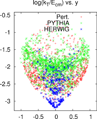
Figure 5: The $\log(k_{T}/\sqrt{s})$ vs. $y$ scatter plot for charm events. We show the results of simulation based on the perturbative three-body matrix element with modified $\alpha_{S}$ (red), PYTHIA (green) and HERWIG (blue).

In fig. 5, we plot the results of HERWIG and PYTHIA, along with the results of simulation based on a perturbative three-body matrix element for $e^{+}e^{-}\to c\bar{c}g$ using the modified $\alpha_{S}$ of ref. odagirihadronization . The choice of the renormalization scale for the perturbative result is $Q^{2}=k_{T}^{2}$. The gluon is identified with the soft particle 3. The peak of $\alpha_{S}$ is at 0.575 GeV. The number of generated events is 1000 for the perturbative case and 10000 for HERWIG and PYTHIA. However, because of the low probability of three-body events, the number of accepted events is much less for both generators.

On the vertical axis, a transverse momentum of 1 GeV corresponds to $\approx-2.3$, and 0.5 GeV corresponds to $\approx-3$. The perturbative distribution is almost flat in rapidity as discussed above, with some modification due to the finite mass.

Turning to the behaviour of the Monte Carlo event generators, we see that the behaviour of the two generators is quite distinct.

The PYTHIA distribution is easier to understand. The band at near 1 GeV, corresponding to $-2$ on the vertical axis, is understood as a combination of the perturbative gluon emission and the artificially generated $p_{T}$, related to the Gaussian width parameters PARJ(21) - PARJ(24).

The HERWIG distribution has a complicated structure. The structure resembling faint lines at $\pm 45$ degrees indicate the typical mass of the cluster that decays into one charmed and one non-charmed meson. The distribution is in general softer than the PYTHIA distribution because the extra particle comes from the decay of a cluster and most of the energy in this decay is taken up by the charmed meson. There is little remnant of perturbative gluon emission since all of the gluons have split into $q\bar{q}$ and these recombine with the colour-connected quark/antiquark to form clusters.

As mentioned at the beginning of this section, the Monte-Carlo predictions should not be trusted for few-body exclusive final states. Nevertheless, the experimental investigation of such configurations can shed light not only on the areas in which the generators could be improved but also on the mechanism of hadronization as a whole. On the other hand, there would be considerable and, seemingly count , not insurmountable difficulty associated with the experimental reconstruction of primary hadrons within the plethora of decay products.

9 Implementation in Herwig++

We now turn to the implementation of the algorithm developed in the previous sections. We choose to adopt Herwig++ hwpp as the platform. The hadronization algorithm of Herwig++ is based on that of HERWIG.

Our implementation entails:

1. Modified daughter mass distribution in cluster decay, generated according to eqn. (36), which can be inverted analytically. We impose ordering in $k_{T}$, and the minimum daughter mass is the sum of the constituent quark masses with the corresponding flavour. Clusters that are too light to be decayed in the default Herwig++ implementation are not decayed.

2. Option of ‘cluster rotation’, or the Regge smearing of the directions of the 3-momenta of the daughter clusters, as well as the partons making up the daughter clusters, with respect to the partons making up the parent cluster. This has the distribution $\propto(\alpha^{\prime}s)^{2\alpha^{\prime}t}$. Here $t$ is the Mandelstam variable for the $(2\to 2)$ subprocess involving, in the initial state, parent cluster partons, and in the final state, the daughter clusters.

3. Option of pomeron inclusion. By imposing the approximation $2\alpha^{\prime}_{\rm Pomeron}=\alpha^{\prime}_{\rm Reggeon}$, the resulting Sudakov form factor is still analytically invertible.

4. Option of Regge flavour and baryon generation taking place after cluster splitting, with weight $\propto(\alpha^{\prime}s)^{2\alpha(0)}$ and adjustable constant multiplicative factor for each flavour and diquark.

In eqn. (36), we use the parametrization:

$$\beta_{H}\equiv\beta/100=1,\quad\alpha^{\prime}=0.9\ \mathrm{GeV}^{-2},\quad\alpha(0)=0.5.$$ (45)

Out of the three parameters, $\alpha^{\prime}$ and $\alpha(0)$ are fixed by Regge phenomenology. The remaining parameter, $\beta_{H}$, is not well determined, but the physical results typically depend only on the logarithm of $\beta_{H}$. This is because the typical $k_{T}$ of cluster decay is the dominant factor in the decay kinematics. The Herwig++ parameter CLPOW becomes redundant. We start by keeping the values of the other parameters the same as in the default set.

All our simulation results are for $e^{+}e^{-}$ interaction at the $Z^{0}$ pole, corresponding to the LEP centre-of-mass energy. We generate 100,000 events in each case. Our simulation results are compared against the default set of experimental data hwppLEPdata in Herwig++. Both soft and hard matrix-element corrections are switched on.

We first show our simulation result for $1-T$ in fig. 6. After including the cluster-rotation effect, the agreement with data is comparable with that of Herwig++, and is better in the region of low $1-T$, corresponding to pencil-like events. We found similar improvement in most other event-shape observables, with the exception of oblateness. For spherical events, not shown in the figure, the results are similar to those obtained using Herwig++.

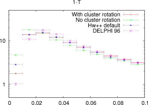
Figure 6: The distribution of $1-T$, with and without the cluster rotation effect.

In addition to the event shapes, we examined the behaviour of the single particle and the identified particle distributions. For the former, the results tend to be better than the Herwig++ numbers for rapidity, but worse for transverse momenta with respect to thrust and sphericity axes. As an example of the latter, fig. 7 shows the in-plane transverse momentum with respect to thrust axis.

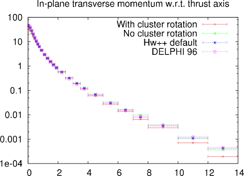
Figure 7: The distribution of in-plane transverse momentum with respect to thrust axis, with and without the cluster rotation effect.

The transverse momentum distributions improve when we omit the cluster rotation, although doing so would ruin the agreement with the event shapes. One speculative possibility would be in the over-generation of transverse momenta in our combined Regge-Herwig++ implementation.

For the identified particle distributions, the results are similar to those of Herwig++. The distribution of scaled momentum of charged particles, shown in fig. 8, shows deficit compared with the experimental data both in the very large-$x_{p}$ and small-$x_{p}$ regions where $x_{p}$ stands for the scaled momentum. For the large-$x_{p}$ region, we find better agreement when the sample is restricted to light-, charm- or bottom-quarks, so that this is possibly not a serious deficit.

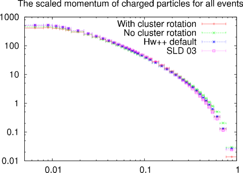
Figure 8: The distribution of the scaled momentum of charged particles, with and without the cluster rotation effect.

In the small-$x_{p}$ region, the agreement is improved by lowering the Herwig++ shower cut-off parameter $\delta$. We found that the flavour dependance of the shower cut-off is milder in our approach. Herwig++ uses the parametrization:

$$Q_{g}=(\delta-0.3m_{q})/2.3,$$ (46)

where $Q_{g}$ is a gluon virtuality cut-off and $\delta$ is constant, but this yields too much radiation from $b$-quarks and too little from light quarks in our approach. The choice of $\delta=2.3$ for $b$-quarks and $\delta=1.7$ for $c$-quarks was found to be more appropriate. An alternative possibility is to introduce the pomeron. We found that the substitution:

$$(\alpha^{\prime}s)^{2\alpha_{\mathrm{Reggeon}}}\longrightarrow(\alpha^{\prime}s)^{2\alpha_{\mathrm{Reggeon}}}+0.02(\alpha^{\prime}s)^{2\alpha_{\mathrm{Pomeron}}},$$ (47)

reproduces the observed charged-particle multiplicity. Doing so, however, leads to the deterioration in the description of the very large-$x_{p}$ region. On the other hand, this deterioration in the large-$x_{p}$ region makes the agreement with the thrust-like event-shape distribution better in the pencil-like region.

The distribution of the proton was found to be in poor agreement with the data and this is similar to the case of Herwig++, but the agreement is better in the case of proton production in charm events. This is shown in fig. 9. This seems to imply that we may have an incomplete description of either the shower cut-off or hadronization in our Regge-Herwig++ amalgamate approach, in the case of the light parton from the hard processs.

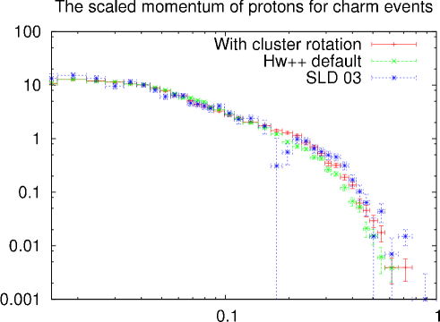
Figure 9: The distribution of the scaled momentum of protons for charm events.

For the last item of our implementation, namely that of flavour generation during cluster decay, we found no visible effect on any of the distributions.

10 Conclusions

We argued that the dynamical conversion of partons to hadrons can be effectively factorized into two phases. The first is an extended perturbative phase based on an universal infrared coupling. The second is a long-distance hadronization phase mediated by colour-singlet resonance–pole dynamics.

From the consideration of the Veneziano $N$-point amplitude, we argued that, essentially because of duality, amplitude-squared factorization is applicable to the latter phase as well as the former phase. This factorization has the form of cascade decay, where each decay except the last one in the chain has Regge angular behaviour.

Since both phases are factorizable, we can describe the overall fragmentation process by merging together the two factorized contributions.

By generalizing the factorization of the $N$-point amplitude, we proposed a framework for Monte-Carlo event generation. We derived an approximate Regge fragmentation function as a special case.

Our results are applicable generally to multiple hadron production from pole–resonance dynamics.

We made a simple implementation of our hadronization algorithm in Herwig++. We found that the event-shapes tend to be better compared with the original procedure. On the other hand, the results are mixed in the case of single-particle and identified-particle distributions.