Extraction of proton form factors in the timelike region
from unpolarized $e^{+}e^{-}\to p\bar{p}$ events

Abstract

We have performed numerical simulations of the unpolarized $e^{+}e^{-}\to p\bar{p}$ process in kinematic conditions under discussion for a possible upgrade of the existing DAFNE facility. By fitting the cross section angular distribution with a typical Born expression, we can extract information on the ratio $|G_{E}/G_{M}|$ of the proton electromagnetic form factors in the timelike region within a 5-10% uncertainty. We have explored also non-Born contributions to the cross section by introducing a further component in the angular fit, which is related to two-photon exchange diagrams. We show that these corrections can be identified if larger than 5% of the Born contribution, and if relative phases of the complex form factors do not produce severe cancellations.

I Introduction

The form factors of hadrons, as obtained in electromagnetic processes, provide fundamental information on their internal structure, i.e. on the dynamics of quarks and gluons in the nonperturbative confined regime. A lot of data for nucleons have been accumulated in the spacelike region using elastic electron scattering (for a review, see Ref. gao and references therein). While the traditional Rosenbluth separation method suggests the well known scaling of the ratio $G_{E}/G_{M}$ of the electric to the magnetic Sachs form factor, new measurements on the electron-to-proton polarization transfer in $\vec{e}^{\,-}p\to e^{-}\vec{p}$ scattering reveal contradicting results, with a monotonically decreasing ratio for increasing momentum transfer $q^{2}=-Q^{2}$ jlab . This fact has stimulated a lot of theoretical work in order to test the reliability of the Born approximation underlying the Rosenbluth method (see Ref. 2gamma1 ; 2gamma2 ; 2gamma3 and references therein), and made it critical to deepen our knowledge of $G_{E}$ and $G_{M}$ also in the timelike region by mapping the $q^{2}$ dependence of their moduli and phases.

Timelike form factors, as they can be explored in $e^{+}e^{-}\to H\bar{H}$ or $p\bar{p}\to\ell^{+}\ell^{-}$ processes, are complex because of the residual interactions of the involved hadrons $H$ (protons $p$). Their absolute values can be extracted by combining the measurement of total cross sections and center-of-mass (c.m.) angular distributions of the final products. The phases are related to the polarization of the involved hadrons (see, e.g., Refs. dubnick ; brodsky1 ; egle1 ).

Experimental knowledge of the form factors in the timelike region is poor (for a review see, for example, Ref. egle1 ). There are no polarization measurements, hence the phases are unknown. The available unpolarized differential cross sections were integrated over a wide angular range, such that the relative weight of $|G_{M}|$ and $|G_{E}|$ is still unknown. In the data analysis, either the hypothesis $G_{E}=0$ or $|G_{E}|=|G_{M}|$ were used. While the former is arbitrary and certainly wrong near the physical threshold $q^{2}=4m^{2}$, with $m$ the nucleon mass, the latter is valid only at $q^{2}=4m^{2}$ but unjustified at larger $q^{2}$. As for the neutron, only one measurement is available by the FENICE collaboration fenice for $q^{2}\leq 6$ GeV², which displays the same previous drawback.

Nevertheless, these few data reveal very interesting properties. The amplitudes in the timelike and spacelike regions are connected by dispersion relations dr . In particular, $|G_{M}|$ should asymptotically become real and scale as in the spacelike region. However, a fit to the existing proton $|G_{M}|$ data for $q^{2}\leq 20$ GeV² is compatible with a size twice as larger as the spacelike results e685-2 . Moreover, the very recent data from the BaBar collaboration on $|G_{E}/G_{M}|$ babar show that the ratio is surprisingly larger than 1, contradicting the spacelike results with the polarization transfer method jlab and the previous timelike data from LEAR lear . Also the few neutron data for $|G_{M}|$ are unexpectedly larger than the proton ones in the corresponding $q^{2}$ range fenice . Finally, all the available data show a steep rise of $|G_{M}|$ at $q^{2}\sim 4m^{2}$, suggesting the possibility of interesting (resonant) structures in the unphysical region (for more details, see Ref. baldini ).

The possible upgrade of the existing DAFNE facility LoI ; roadmap to enlarge the c.m. energy range from the $\phi$ mass to 2.5 GeV with a luminosity of at least $10^{32}$ cm^-2s^-1, would allow to explore with great precision the production of baryon-antibaryon pairs from the nucleon up to the $\Delta$.

In the following, in Sec. II we briefly review the formalism necessary to extract absolute values and phases of baryon timelike form factors from cross section data. In Sec. III, we outline the main features of our Monte Carlo simulation for the measurement of proton form factors. In Sec. IV, we focus on unpolarized $p\bar{p}$ production, and in particular on the relevant problem of a precise extraction of the ratio $r_{e}\equiv|G_{E}/G_{M}|$ from the $\cos^{2}\theta$ term of the expected event distribution at any given $q^{2}$. The single-polarized case will be discussed elsewhere next . In Sec. V, we apply the same procedure to identify the presence of a contamination in the unpolarized event distribution by processes beyond the Born approximation, in particular contributions from two-photon ($2\gamma$) exchange. Some concluding remarks are given in the final Sec. VI.

II General formalism

The scattering amplitude for the reaction $e^{+}e^{-}\to B\bar{B}$, where an electron and a positron with momenta $k_{1}$ and $k_{2}$, respectively, annihilate into a spin-$\textstyle{\frac{1}{2}}$ baryon and an antibaryon with momenta $p_{1}$ and $p_{2}$, respectively, is related by crossing to the corresponding scattering amplitude for elastic $e^{-}B$ scattering. In the timelike case, and in presence of a possible $2\gamma$ exchange term, quite a few independent real scalar functions are required to describe the process. There are several equivalent representations of them; here, we use the one involving the axial current following the scheme of Ref. egle2 . The scattering amplitude can be fully parametrized in terms of three complex form factors: $G_{E}(q^{2},t),\,G_{M}(q^{2},t),$ and $G_{A}(q^{2},t)$, which are functions of $q^{2}=(k_{1}+k_{2})^{2}$ and $t=(k_{2}-p_{1})^{2}$. They refer to an identified baryon-antibaryon pair in the final state, rather than to an identified isospin state. In the following, we will use $\cos\theta$ instead of the variable $t$, with $\theta$ the angle between the momenta of the positron and the recoil proton in the c.m. frame.

In the Born approximation, $G_{E}$ and $G_{M}$ reduce to the usual Sachs form factors and they do not depend on $\cos\theta$, while $G_{A}=0$. For the construction of our Monte Carlo event generator, we rely on the general and extensive relations of Ref. egle2 up to the single polarization case. These relations assume small non-Born terms and include them up to order $\alpha^{3}$ (with $\alpha$ the fine structure constant), i.e. they consider $2\gamma$ exchange only via their interference with the Born amplitude. These corrections introduce explicitly six new functions, that all can depend on $\cos\theta$: the real and imaginary parts of $\Delta G_{E}$ and $\Delta G_{M}$, i.e. the $2\gamma$ corrections to the Born magnetic and electric form factors, and the real and imaginary parts of the axial form factor $G_{A}$. The role of these corrections in the unpolarized and single polarized cross sections is very simple: it can be deduced from the Born term by adding the contribution of $G_{A}$ and substituting the Born form factors with the ”$2\gamma-$improved” form factors, i.e. $G_{E,M}(q^{2})$ $\rightarrow$ $G_{E,M}(q^{2})+\Delta G_{E,M}(q^{2},cos\theta).$ In Ref. egle2 , this fact is somehow hidden by neglecting terms of order $\alpha^{4}$. However, for sake of simplicity we keep $2\gamma$ effects via the axial form factor only. Within this scheme, when summing events with positive and negative polarization, the unpolarized cross section can be written as

$$\frac{d\sigma^{o}}{d\cos\theta} = a(q^{2})\,[1+R(q^{2})\,\cos^{2}\theta]-b(q^{2})\,\mathrm{Re}[G_{M}(q^{2})\,{G_{A}}^{\ast}(q^{2},\cos\theta)]\,\cos\theta\;,$$ (1)

$$a(q^{2}) = \frac{\alpha^{2}\pi}{2q^{2}}\,\frac{1}{\tau}\,\sqrt{1-\frac{1}{\tau}}\,\left(\tau|G_{M}|^{2}+|G_{E}|^{2}\right)\;,\quad b(q^{2})=\frac{2\pi\alpha^{2}}{q^{2}}\,\frac{\tau-1}{\tau}\;,$$ (2)

$$R(q^{2}) = \frac{\tau|G_{M}(q^{2})|^{2}-|G_{E}(q^{2})|^{2}}{\tau|G_{M}(q^{2})|^{2}+|G_{E}(q^{2})|^{2}}\;,\quad\tau=\frac{q^{2}}{4m^{2}}\;.$$ (3)

Measurements of the unpolarized cross section at fixed $q^{2}$ for different values of $\theta$ allow us to fit the different $\cos^{n}\theta$ terms, from which we can extract $|G_{E}/G_{M}|$ and some information on $G_{A}(q^{2},cos\theta)$.

For spin-$\textstyle{\frac{1}{2}}$ baryons with polarization $\mathbf{S}_{B}$, the cross section is linear in the spin variables, i.e. $d\sigma=d\sigma^{o}\,(1+\mathcal{P}\,\mathcal{A})$, with $d\sigma^{o}$ from Eq. (1) and $\mathcal{A}$ the analyzing power. In the c.m. frame, three polarization states are observable dubnick ; brodsky1 : the longitudinal $\mathcal{P}_{z}$, the sideways $\mathcal{P}_{x}$, and the normal $\mathcal{P}_{y}$. The first two ones lie in the scattering plane, while the normal points in the $\mathbf{p}_{1}\times\mathbf{k}_{2}$ direction, the $x,y,z,$ forming a right-handed coordinate system with the longitudinal $z$ direction along the momentum of the outgoing baryon. The $\mathcal{P}_{y}$ is particularly interesting, since it is the only observable that does not require a polarization in the initial state dubnick ; brodsky1 . With the above approximations, it can be deduced by the spin asymmetry between events with positive and negative normal polarizations:

$$\mathcal{P}_{y}=\frac{1}{\mathcal{A}_{y}}\,\frac{d\sigma^{\uparrow}-d\sigma^{\downarrow}}{d\sigma^{\uparrow}+d\sigma^{\downarrow}}=\frac{b(q^{2})}{2\sqrt{\tau-1}\,d\sigma^{o}}\,\sin\theta\,\Big{\{}\cos\theta\,\mathrm{Im}\left[G_{M}(q^{2})\,G_{E}^{\ast}(q^{2})\right]-\sqrt{\frac{\tau-1}{\tau}}\,\mathrm{Im}\left[G_{E}(q^{2})\,{G_{A}}^{\ast}(q^{2},\cos\theta)\right]\Big{\}}\;.$$ (4)

This spin asymmetry can be nonvanishing even without polarized lepton beams, because it is produced by the mechanism $\mathbf{p}_{1}\times\mathbf{k}_{2}\cdot\mathbf{S}_{B}$, which is forbidden in the Born approximation for the spacelike elastic scattering brodsky1 . However, the measurement of $\mathcal{P}_{y}$ alone does not completely determine the phase difference of the complex form factors. By defining with $\delta_{E}$ and $\delta_{M}$ the phases of the electric and magnetic form factors, respectively, the Born contribution is proportional to $\sin(\delta_{M}-\delta_{E})$, leaving the ambiguity between $(\delta_{M}-\delta_{E})$ and $\pi-(\delta_{M}-\delta_{E})$. Only the further measurement of $\mathcal{P}_{x}$ can solve the problem, because $\mathcal{P}_{x}\propto\mbox{\rm Re}(G_{M}\,G_{E}^{\ast})\propto\cos(\delta_{M}-\delta_{E})$ brodsky1 . But at the price of requiring a polarized electron beam.

III General features of the numerical simulation

We consider the $e^{+}e^{-}\to p\bar{p}$ process. Events are generated in the variables $q^{2},\,\theta,\,\phi$ (the azimuthal angle of the proton momentum with respect to the scattering plane), and $S_{y}$ (the proton polarization normal to the scattering plane). Then, the distribution is summed upon the spin and integrated upon $\phi$.

The exchanged timelike $q^{2}$ is fixed by the beam energy. Only the scattering angle $\theta$ is randomly distributed. For a given $q^{2}$, the Born term is responsible for the $[1+R(q^{2})\,\cos^{2}\theta]$ behaviour of the event distribution. Since at this level and with the discussed approximations no other dependence in $\theta$ is present, observed systematic deviations from the $[1+R(q^{2})\,\cos^{2}\theta]$ behaviour will be interpreted as a clear signature of non-Born terms.

An overall sample of $300\,000$ events has been considered with $3.8\leq q^{2}\leq 6.2$ GeV² and $|\cos\theta|<0.9$. Since the integrated cross section for $e^{+}e^{-}\to p\bar{p}$ in the considered region is approximately 1 nb, at the foreseen luminosity of $10^{32}$ cm^-2s^-1 this sample can be collected in one month with efficiency 1. The upper $q^{2}$ cutoff is consistent with the upper limit of the c.m. energy in the presently discussed upgrade of DAFNE LoI ; roadmap . The lower limit includes the $p\bar{p}$ threshold, but in our simulation we avoid this region which is characterized by peculiar mechanisms like, e.g., the Coulomb focussing and possible subthreshold resonances.

Results depend much on the binning of the events. In fact, while a larger number of bins in the same $(q^{2},\theta)$ region implies a more precise determination of $q^{2}$ and $\theta$, at the same time it leaves each bin with much less events and, consequently, with larger error bars. We find the best compromise with 6 equally spaced $q^{2}$ bins with width $\Delta q^{2}=0.4$ GeV², and 7 equally spaced $\cos\theta$ bins with width $\Delta\cos\theta\approx 0.257$ for the solid angle $|\cos\theta|<0.9$. Incidentally, we notice that with $\Delta q^{2}=0.4$ GeV² the deviation inside each bin between the statistical average $q^{2}$, calculated in the simulation, and the central value $(q^{2}_{max}-q^{2}_{min})/2$ is about 3%.

Since it is well known that $|G_{M}(q^{2})|\sim 1/q^{4}$ brodsky , from Eqs. (1-3) we expect the cross section to approximately fall like $1/q^{10}$. This implies that bins at higher $q^{2}$ are scarcely populated. For example, out of the $300\,000$ selected events only 700 are accumulated in the $5.8\leq q^{2}\leq 6.2$ GeV² range for each $\cos\theta$ bin. In these conditions, a gaussian fluctuation of $1\sigma$ differs by 5% from the average value; therefore, deviations of at least 10% from the Born cross section are needed to be recognized as systematic effects due to non-Born terms. The situation is evidently more favourable at lower $q^{2}$: in the $3.8\leq q^{2}\leq 4.2$ GeV² range around $23\,000$ events are accumulated in each $\cos\theta$ bin. Of course, it could be possible to asymmetrically split the beam time in order to make the statistics of each $q^{2}$ bin more homogeneous. More importantly, since in a $e^{+}e^{-}$ collider experiment $q^{2}$ is fixed by the colliding particle energy, it could be more convenient to concentrate on narrow subranges like, e.g., $4\leq q^{2}\leq 4.1$ GeV² and $4.4\leq q^{2}\leq 4.5$ GeV². The reconstruction efficiency does not change much when the same number of events is concentrated in two bins centered around the same $q^{2}$ value but with different widths $\Delta q^{2}$, at least for $\Delta q^{2}\ll 1$ GeV². We define as ”default conditions” the ones where the whole possible range in $q^{2}$ is divided in equally spaced bins and each one is sampled with the same beam time; our results are presented in this framework. A discussion about other possible choices is beyond the scope of this paper.

Events can be generated only by inserting specific parametrizations of the proton form factors in the cross section. For $G_{E}$ and $G_{M}$, several models can be considered in the timelike region brodsky1 ; egle1 , mostly derived from extrapolations from the spacelike region. We selected the parametrizations of Refs. iachello ; lomon , because they have been recently updated in Ref. egle1 by simultaneously fitting both the spacelike and timelike available data. Moreover, both cases release separate parametrizations for the real and imaginary parts of $G_{E}$ and $G_{M}$. We indicate the former as the IJLW parametrization (from the initials of their authors), and the latter as the Lomon parametrization.

Since the explored $q^{2}$ range is not large, it is reasonable to make also much simpler, but equally effective, choices. Accordingly, we use also a parametrization where all form factors are real and proportional to the same dipole term $1/(1+q^{2}/q_{o}^{2})^{2}$, with $q_{o}=0.71$ GeV, as in the spacelike region. This choice looks reasonable also for $G_{A}$, of which nothing can be said except that hopefully its modulus could have the same dipole trend in the considered $q^{2}$ range. All form factors being proportional to the same function, the actual parameters are the ratios $r_{e}=|G_{E}/G_{M}|$ and $r_{a}=|G_{A}/G_{M}|$, and the relative phases $\beta_{e}$ and $\beta_{a}$ of $G_{E}$ and $G_{A}$, respectively, with respect to $G_{M}$; they determine the sign of the corresponding ratios. We will refer to the parametrization Dip0 when $r_{e}=r_{a}=0$; to Dip1 when $r_{e}=1$ and $r_{a}=0$; to Dip$2\gamma$ when $r_{e}=1$ and $r_{a}=0.2$. Since the Born term in the cross section depends only on $|G_{E}|^{2}$ and $|G_{M}|^{2}$, we can safely take $\beta_{e}=0$. We refer the reader to Sec. V for a discussion about $r_{a}$ and $\beta_{a}$.

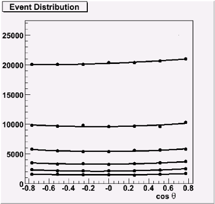
Figure 1: Angular distribution of $300\,000$ events for the $e^{+}e^{-}\to p\bar{p}$ process at $3.8\leq q^{2}\leq 6.2$ GeV² and $|\cos\theta|<0.9$, and with the Dip1 parametrization of proton form factors (see text). The points correspond to 7 equally spaced $\cos\theta$ bins for each of 6 equally spaced $q^{2}$ bins. Solid curves are the results of a 3 parameters angular fit with $B\propto r_{a}=|G_{A}/G_{M}|=0$ (see text). The highest curve corresponds to the lowest bin $3.8\leq q^{2}\leq 4.2$ GeV²; next lower curve to the adjacent bin $4.2\leq q^{2}\leq 4.6$ GeV², and so on.

IV Reconstruction of $|G_{E}/G_{M}|$

As already stressed in the Introduction, one of the puzzling features of the available data is that the BaBar collaboration reports a value for $|G_{E}/G_{M}|$ bigger than 1 in the timelike region babar , which contradicts the spacelike results jlab and the previous timelike data from LEAR lear . Therefore, it is important to explore the possibility of new and more precise measurements of $|G_{E}/G_{M}|$ in the unpolarized $e^{+}e^{-}\to p\bar{p}$ process at the upgraded DAFNE LoI ; roadmap .

Our analysis consists of three steps; for sake of simplicity, we describe it in the following for the case of the parametrization Dip1:

• We generate $300\,000$ events for $3.8\leq q^{2}\leq 6.2$ GeV² and $|\cos\theta|<0.9$ (i.e., for $25^{\mathrm{o}}\leq\theta\leq 155^{\mathrm{o}}$). The sorted events are divided into 6 equally spaced $q^{2}$ bins of width $\Delta q^{2}=0.4$ GeV². In each $q^{2}$ bin, the events are divided into 7 equally spaced $\cos\theta$ bins with width $\Delta\cos\theta\approx 0.257$. In Fig. 1, the points show the 6 distributions in $q^{2}$, each one consisting of 7 points describing the distribution in $\cos\theta$. From the discussion in the previous section, the highest $\cos\theta$ distribution corresponds to the lowest bin $3.8\leq q^{2}\leq 4.2$ GeV²; the next lower distribution to the adjacent bin $4.2\leq q^{2}\leq 4.6$ GeV², and so on.

  

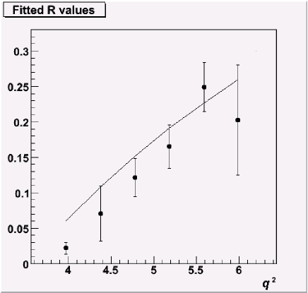
  Figure 2: Fitted $R$ values from the event distribution of Fig. 1, according to Eq. (5) (see text). Solid line represents the expected values for the Dip1 parametrization according to Eq. (6) (see text).

• For each $q^{2}$ bin, the $\cos\theta$ dependence of the event distribution is fitted by a function of the form

  $$N(\cos\theta)=\ A\Big{(}1\ -\ B\,\cos\theta\ +\ R\,\cos^{2}\theta\Big{)}\;,$$ (5)

  with three fitting parameters $A,B$, and $R$. The results of each fit are represented by the solid curves in Fig. 1. The parameter $A$ is not crucial for the following discussion and it will not be considered. The parameter $B$ contains the effects of $2\gamma$ exchange which will be discussed in Sec. V. Here, we just notice that, with the input $r_{a}=|G_{A}/G_{M}|=0$ and discarding $2\gamma$ effects in $G_{E}$ and $G_{M}$, the simulation produces almost perfectly symmetric curves in $\cos\theta$, indicating that within the statistical uncertainty $B\sim 0$, as expected. The parameter $R$ must obviously be identified with the function $R(q^{2})$ of Eq. (3), and it is related to $r_{e}=|G_{E}/G_{M}|$ by

  $$R\ =\ \frac{\tau-r_{e}}{\tau+r_{e}}\;.$$ (6)

  The fitted $R$ values are reported in Fig. 2 against the corresponding average $q^{2}$ values of each bin. The error bars are the output of the fitting procedure, i.e. they represent the uncertainty in determining $R$ when using the form (5) to fit the event distribution in Fig. 1. The solid curve in Fig. 2 represents the expected value of $R$ when the Dip1 parametrization for the form factors is inserted in Eq. (6) through $r_{e}$.

  

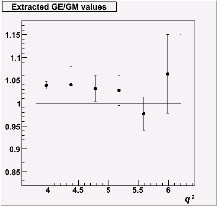
  Figure 3: Extracted $r_{e}=|G_{E}/G_{M}|$ values from the event distribution of Fig. 1. Solid line gives the expected value according to the Dip1 parametrization (see text).

• If we define $\Delta R$ as half of the error bar associated with a given $R$ value in Fig. 2, we can also define the pair $(R_{min}=R-\Delta R,\,R_{max}=R+\Delta R)$. By inverting the relation (6), it is possible also to deduce the corresponding pair $(r_{e_{min}},\,r_{e_{max}})$, which can be transformed into $(r_{e},\Delta r_{e})$ with $\Delta r_{e}=(r_{e_{max}}-r_{e_{min}})/2$. These extracted values of $r_{e}=|G_{E}/G_{M}|$ and the associated error bars $\Delta r_{e}$ are displayed for each corresponding $q^{2}$ bin in Fig. 3. The solid line represents the expected $r_{e}$ value (in this case, $r_{e}=1$ because we are using the Dip1 parametrization). The comparison between expected and reconstructed $r_{e}$ values displays the potential reliability of the measurement of $r_{e}$ with a sample of $300\,000$ events and with the chosen binning in $q^{2}$.

Our reconstruction procedure is based on the structure of the cross section (1), which naturally suggests to fit the directly observable parameter $R$ and then to link it to $r_{e}$ according to Eq. (6). It must be remarked that the usual formula for the error propagation cannot be used to derive $\Delta r_{e}$ from $\Delta R$, because for some $R$ values the relative error is very large (see Fig. 2). We stress that the error bars are related to the fitting procedure, i.e. they give the integral deviation between the test function (5) and the data points. They are not directly related to the statistical errors on the average population of each bin. In the measurement of a really random variable, in the limit of infinite number of events, the statistical error on the population of a single bin tends to vanish because of the central limit theorem. In the same limit, the error from the fitting procedure does not tend to vanish unless the number of parameters is equal to the number of bins (in this case, 7 $\cos\theta$ bins for each independent fitting procedure). Anyway, the statistical fluctuations can be estimated from the distance between expected and reconstructed $r_{e}$ values.

In order to extract $r_{e}$ from $R$ we need to assign a common $\tau$ value, i.e. $q^{2}$, to all the events falling into a specific $q^{2}$ bin. Integrating over all the generated events, we have calculated the average $q^{2}$ for each $q^{2}$ bin, and used it for the extraction of $r_{e}$. We recall that this average $q^{2}$ differs by about 3% from the central value $(q^{2}_{max}-q^{2}_{min})/2$ deduced from the bin width $\Delta q^{2}=q^{2}_{max}-q^{2}_{min}$.

It is important to notice also that, despite the large number of available events, the region with the smallest $q^{2}$ is delicate. In fact, $R$ is small but has not a small derivative in $q^{2}$ near threshold. This reflects in a striking contrast between the very small fitting error bar, on one side, and a worse comparison between reconstructed and expected $r_{e}$ than at larger $q^{2}$, on the other side.

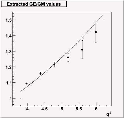
Figure 4: Extracted $r_{e}=|G_{E}/G_{M}|$ values from the event distribution in the same conditions as in Fig. 1 but for the IJLW parametrization of Ref. iachello , as updated in Ref. egle1 (see text). Solid line is the expected result.

We have repeated the reconstruction procedure also for the Dip0 parametrization, i.e. for $r_{e}=|G_{E}/G_{M}|=0$, which has been used in some experiments to extract the timelike $|G_{M}|$ data from unpolarized cross section measurements. The comparison between expected and reconstructed $r_{e}$ is more difficult, because not only the fitting error is obviously larger, but also the statistical one. However, since the considered $q^{2}$ are rather close to the physical threshold, $|G_{E}/G_{M}|$ may not be very different from its threshold value of unity. According to the results with the Dip1 parametrization, this should simplify the task of a precise extraction of $r_{e}$ in a real experiment.

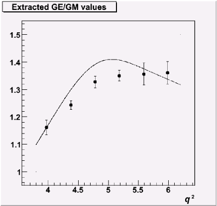
Figure 5: Extracted $r_{e}=|G_{E}/G_{M}|$ values from the event distribution in the same conditions as in Fig. 1 but for the Lomon parametrization of Ref. lomon , as updated in Ref. egle1 (see text). Solid line is the expected result.

To verify this conjecture, we have repeated the procedure starting from the realistic parametrizations IJLW (Fig. 4) and Lomon (Fig. 5). Again, the solid curves show the expected values of $r_{e}$ as calculated for each different choice.

Three peculiar features distinguish these two examples from the previous ones: $G_{E}$ and $G_{M}$ are complex objects; $r_{e}$ is not a constant; it is close to 1 but bigger than 1, in agreement with the recent findings of the BaBar experiment babar . In both cases, the quality of the reconstruction of $r_{e}$ is very good, confirming that in most of the $q^{2}$ bins the extraction of $|G_{E}/G_{M}|$ is possible with an accuracy within 10% for the considered sample and binning. This is mainly due to the simple dependence of the $\cos^{2}\theta$ term in the angular distribution upon only one parameter, i.e. $r_{e}=|G_{E}/G_{M}|$; to the neglect of more complicated angular terms, like $\cos^{4}\theta$; and to the vicinity of $q^{2}$ to the physical threshold $q^{2}=4m^{2}$, which implies $|G_{E}/G_{M}|\sim 1$.

V The two-photon contribution

As already anticipated in Sec. II, we account for non-Born contributions to the unpolarized cross section only through the axial form factor $G_{A}$. According to the Dip$2\gamma$ parametrization discussed in Sec. IV, $G_{A}$ is modeled as

$$G_{A}(q^{2},\cos\theta)\ =\ r_{a}\,e^{i\beta_{a}\pi}\,G_{M}(q^{2})\;,$$ (7)

where we neglect any explicit dependence on $\cos\theta$. We take $G_{M}$ real and with the dipole form. Indeed, in the kinematical region under analysis the ratio $G_{E}/G_{M}$ is complex, but most likely dominated by its real part. A nonvanishing phase is due to the reinteraction between the two hadrons in the final state. Very close to the threshold (i.e., in a relative $s$ wave) the phenomenon presents peculiar features, but from the onset of the $p$ wave contribution onwards, an approximately semiclassical black-disk regime takes over pbar1 . In these conditions, the main effect of the $p\bar{p}$ interaction is a flux damping. The transition from the near-threshold to the black-disk regime is signalled by the change of sign of the $\rho$ parameter, i.e. the ratio between the real and imaginary parts of the forward $p\bar{p}$ scattering amplitude. Such a transition takes place below the $q^{2}$ range considered in our analysis. In the black-disk regime, it is natural to think that the flux absorption leads to the appearance of an imaginary part for $G_{E}$ and $G_{M}$. However, the absorption cross section is much below the unitarity limit, suggesting that the phases of $G_{E}$ and $G_{M}$ may be small. For $G_{A}$ it is not possible to conclude that it is ”quasi-real”. $|G_{A}|$ is presumably small, and the cuts on the two-photon lines involving all the possible on-shell intermediate states in the amplitude, may produce a relevant imaginary part.

The $G_{A}$ form factor enters the unpolarized cross section with a contribution proportional to $\cos\theta\,\mathrm{Re}(G_{M}G_{A}^{*})$. Therefore, we can have

$$\mathrm{Re}[G_{M}\,G_{A}^{*}]\approx G_{M}\,\mathrm{Re}[G_{A}^{*}]\approx r_{a}\,\cos\beta_{a}\pi\,G_{M}^{2}\equiv rr_{a}\,G_{M}^{2}\;.$$ (8)

In our simulation with the Dip$2\gamma$ parametrization, we consider $G_{M},\,G_{E}$, and $G_{A}$, all real functions of $q^{2}$, with $r_{e}=|G_{E}/G_{M}|=1$ and $rr_{a}\approx r_{a}=|G_{A}/G_{M}|=0.2$, i.e. with $\beta_{a}=0$. This is the most optimistic situation we may guess, taking into account that: (i) no realistic models are available for $G_{A}$; (ii) in the spacelike case, the assumption that $r_{a}$ is at most 0.2 does not contradict the data; (iii) in the timelike case, $G_{A}$ should have a nonvanishing phase.

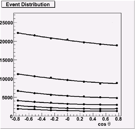
Figure 6: Angular distributions for $300\,000$ events for the $e^{+}e^{-}\to p\bar{p}$ process in the same conditions as in Fig. 1, but for $r_{a}=|G_{A}/G_{M}|=0.2$.

In Fig. 6, the generated events are sorted in $q^{2}$ and $\cos\theta$ bins as in Fig. 1. We can see now that $2\gamma$ effects show up in a marked left-right asymmetry of points in $\cos\theta$. The solid curves are obtained from the fitting formula (5), where now the parameter $B$ is given by

$$B(q^{2})\ =\ r_{a}\,f(q^{2},r_{e})\;,$$ (9)

with

$$f(q^{2},r_{e})\ =4\frac{\sqrt{\tau(\tau-1)}}{\tau+r_{e}^{2}}\;.$$ (10)

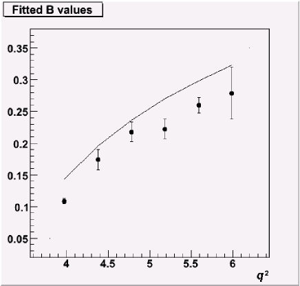
Figure 7: Fitted $B$ values from the event distributions of Fig. 6 according to Eq. (5) (see text). Solid line represents the expected value for the Dip$2\gamma$ parametrization according to Eq. (9) (see text).

In Fig. 7, the fitted values of $B$ and the relative errors are shown. As usual, the solid line shows the expected result, by inserting $r_{e}=1$ and $r_{a}=0.2$ in Eqs. (9-10).

In order to estimate $r_{a}$ from $B$, we assume small errors for both $B$ and $r_{e}$, with the caveat that such an assumption is not valid near the lowest $q^{2}$ threshold. Using the formula for the systematic error propagation, we get

$$\Delta r_{a}\ =\ \frac{r_{a}}{B}\,\left[\Delta B+\ \frac{2r_{e}}{\tau+r_{e}^{2}}\,B\,\Delta r_{e}\right]\;.$$ (11)

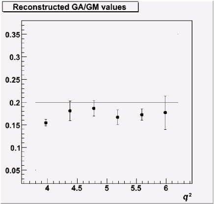
Figure 8: Extracted $r_{a}=|G_{A}/G_{M}|$ values from the event distributions of Fig. 6 according to the Dip$2\gamma$ parametrization; solid line is the expected result (see text).

In Fig. 8, the $r_{a}$ values, reconstructed from Eq. (9), are shown together with the relative errors $\Delta r_{a}$ from Eq. (11). The solid line is the expected value $r_{a}=0.2$. From the figure it is evident that the error bars (fitting errors) and the discrepancy from the expected value (statistical errors) are of magnitude $2\Delta r_{a}\sim 0.05$. Therefore, with the considered sample and binning we would be able to distinguish a non-Born contribution when it is of the size $|r_{a}|>0.05$.

The additional non-Born corrections to $G_{E}$ and $G_{M}$ can be effectively reabsorbed in the measurement of the left-right asymmetry in the $\cos\theta$ distribution. As shown in Ref. 2gamma3 , charge conjugation invariance imposes general symmetry properties of the Born and $2\gamma$ amplitudes with respect to the $\cos\theta\rightarrow-\cos\theta$ transformation. In particular, the $2\gamma$ corrections to the form factors should respect the following constraints

$$\Delta G_{E,M}(q^{2},\cos\theta)=-\Delta G_{E,M}(q^{2},-\cos\theta)\;,\qquad G_{A}(q^{2},\cos\theta)=G_{A}(q^{2},-\cos\theta)\;.$$ (12)

It follows that the contribution of the $\mathrm{Born}\otimes 2\gamma$ interference term to the unpolarized cross section has the general expression

$$\frac{d\sigma^{\mathrm{(int)}}}{d\cos\theta}=\cos\theta\,[c_{0}(q^{2})\ +\ c_{1}(q^{2})\,\cos^{2}\theta\ +\ c_{2}(q^{2})\,\cos^{4}\theta\ +\ \dots]\;,$$ (13)

where $c_{i}$ $(i=0,1,\dots)$ are real coefficients incorporating effects from all the three different form factors. In our analysis, where we take $\Delta G_{E,M}=0$ and we consider only the first term in the power expansion in $\cos\theta$ of $G_{A}$, the left-right asymmetry proportional to $r_{a}$ gives us only a lower bound for the actual strength of the $2\gamma$ effects. It is however evident that several independent observables, including the polarization of the recoil proton and/or electron beam, are necessary to disentangle the two-photon contribution from each of the three form factors.

VI Conclusions

We have performed numerical simulations of the $e^{+}e^{-}\to p\bar{p}$ unpolarized process using a sample of $300\,000$ events in the kinematical region with $3.8\leq q^{2}\leq 6.2$ GeV², distributed over 6 equally spaced bins. For each $q^{2}$ bin, events were further distributed over 7 equally spaced bins in $\cos\theta$, with $|\cos\theta|<0.9$. For each $q^{2}$ value, the distribution in $\cos\theta$ was fitted by the function $A[1\ -\ B\cos\theta\ +\ R\cos^{2}\theta]$, where the fit parameters $R$ and $B$ allow for the reconstruction of the underlying values of the ratio $r_{e}\equiv|G_{E}/G_{M}|$ and $r_{a}\equiv|G_{A}/G_{M}|$, respectively, once models for the proton form factors are inserted as input.

Concerning $r_{e}$, the reconstruction seems to be relatively simple if $G_{E}\sim G_{M}$, as we expect in the considered kinematical range. The size of the sample reproduces the expected $|G_{E}/G_{M}|$ within 5-10%. The worst performance is for $q^{2}\approx 6$ GeV², where the bins are more scarcely populated.

The additional contributions related to two-photon exchange diagrams show up in a left-right asymmetry of the angular distribution, driven by the parameter $B$. In our analysis, we modeled such a contribution in terms of the axial form factor $G_{A}$, providing a lower bound for the actual strength of two-photon effects. The simulation shows that it is possible to identify and estimate this term, if $|G_{A}|$ (or equivalently $|\Delta G_{E}|$ or $|\Delta G_{M}|$) is larger than 5% of $|G_{M}|$, and the relative phases of the form factors do not combine in such a way to produce severe cancellations. However, a more refined analysis, simultaneously including also polarization observables, is needed to better constrain and disentangle the two-photon contribution from each of the three form factors.

References

-
(1)
C.E. Hyde-Wright and K. De Jager,
Ann.Rev.Nuc.Part.Sci. 54, 217 (2004);
H. Gao, Int. J. Mod. Phys. E12, 1 (2003) [Erratum-ibid E12, 567 (2003)];
I.A. Qattan et al. [JLab Hall A], Phys. Rev. Lett. 94, 142301 (2005). -
(2)
V. Punjabi et al. [JLab Hall A],
Phys. Rev. C71, 055202 (2005)
[Erratum-ibid 71, 069902 (2005)];
O.Gayou et al. [JLab Hall A], Phys. Rev. Lett. 88, 092301 (2002);
M.K.Jones et al. [JLab Hall A], Phys. Rev. Lett. 84, 1398 (2000). - (3) A.V. Afanasev et al., Phys. Rev. D72, 013008 (2005).
- (4) P.G. Blunden, W. Melnitchouk, and J.A. Tjon, Phys. Rev. C72, 034612 (2005).
- (5) M.P. Rekalo and E. Tomasi-Gustafsson, Eur. Phys. J. A22, 331 (2004).
- (6) A.Z. Dubnickova, S. Dubnicka, and M.P. Rekalo, Nuovo Cimento A109, 241 (1996).
- (7) S.J. Brodksy et al., Phys. Rev. D69, 054022 (2004).
- (8) E. Tomasi-Gustafsson et al., E. Phys. J. A24, 419 (2005).
- (9) A. Antonelli et al. [FENICE], Nucl. Phys. B517, 3 (1998).
-
(10)
P. Mergell, U.-G. Meissner, and D. Drechsel,
Nucl. Phys. A596, 367 (1996);
H.-W. Hammer, U.-G. Meissner, and D. Drechsel, Phys. Lett. B385, 343 (1996). - (11) M. Andreotti et al. [E685], Phys. Lett. B559, 20 (2003).
- (12) B. Aubert et al. [BaBar], Phys. Rev. D73, 012005 (2006).
- (13) B. Bardin et al. [LEAR], Nucl. Phys. B411, 3 (1994).
- (14) R. Baldini et al., Eur. Phys. J. C11, 709 (1999).
-
(15)
N. Apokov et al.,
Measurement of the Nucleon Form Factors in the Time-Like region at DAFNE,
Letter of Intent (October 2005), see http://www.lnf.infn.it/conference/nucleon05/loi06.pdf - (16) F. Ambrosino et al., Prospects for physics at Frascati between the and the , hep-ex/0603056.
- (17) A. Bianconi, B. Pasquini, and M. Radici, in preparation.
- (18) G.I. Gakh and E. Tomasi-Gustafsson, Nucl. Phys. A771, 169 (2006).
-
(19)
S.J. Brodsky and G.P. Lepage,
Phys. Rev. D24, 2848 (1981);
S.J. Brodsky and G.R. Farrar, Phys. Rev. D11, 1309 (1975). -
(20)
F. Iachello, A.D. Jackson, and A. Lande,
Phys. Lett. B43, 191 (1973);
F. Iachello and Q. Wan, Phys. Rev. C69, 055204 (2004). - (21) E.L. Lomon, Phys. Rev. C66, 045501 (2002).
-
(22)
A. Bianconi et al.,
Phys.Lett. B483, 353 (2000);
G. Bendiscioli and D. Kharzeev, Rivista del Nuovo Cimento 17, 1 (1994).