Electroweak Phase Transition and Baryogenesis in the nMSSM

Abstract

We analyze the nMSSM with CP violation in the singlet sector. We study the static and dynamical properties of the electroweak phase transition. We conclude that electroweak baryogenesis in this model is generic in the sense that if the present limits on the mass spectrum are applied, no severe additional tuning is required to obtain a strong first-order phase transition and to generate a sufficient baryon asymmetry. For this we determine the shape of the nucleating bubbles, including the profiles of CP-violating phases. The baryon asymmetry is calculated using the advanced transport theory to first and second order in gradient expansion presented recently. Still, first and second generation sfermions must be heavy to avoid large electric dipole moments.

I Introduction

Lately, electroweak baryogenesis (EWBG) Kuzmin:1985mm has again attracted more attention, not least because new collider data will hopefully provide information about the relevant (supersymmetric?) physical parameters in the next years.

Electroweak baryogenesis relies on a strong first-order electroweak phase transition as the source of out-of-equilibrium effects. During a first-order phase transition, bubbles of the low-temperature (broken) phase nucleate and expand to fill all space. An important aspect in the determination of the baryon asymmetry is the impact of transport phenomena Cohen:1994ss . Without transport, CP-violating currents would only be generated near the bubble wall profile of the Higgs vevs. Close to the wall, sphaleron transitions are already strongly suppressed by the mass of the W-bosons, so that B-violating processes are inefficient in producing the observed baryon asymmetry (BAU). Early works that incorporated transport effects into the EWBG calculus were based on the WKB approach Joyce:1994fu . In this framework, a CP-violating shift in the dispersion relation induces a force of second order in the gradient expansion in the Boltzmann equation and leads to CP-violating fermion densities in the symmetric phase. Later on, this formalism was applied to the MSSM, where CP violation results from mixing effects in the chargino sector JCK . In this context, the formalism had to be extended to the case of mixing fermions. In the MSSM, the second-order source is too weak to yield a successful baryogenesis Kainulainen:2001cn ; kpss .

One disadvantage of the WKB method is the neglect of dynamical flavor mixing effects. While the shift in the dispersion relation is due to mixing of left- and right-handed components of the fermions and already present in the one-flavor case, flavor mixing contributions have been completely neglected after a flavor basis transformation to the mass eigenbasis. A series of papers cmqsw ; cmqsw2 aimed at improving on this point by including flavor mixing by using a perturbative expansion of the Kadanoff–Baym equations. Here, the deviations of the Green function have been interpreted as sources in the diffusion equation. This approach — like the WKB-approach — has the weakness that the transport equations only describe the dynamics of two classical quasi-particles in the chargino sector. CP violation is communicated from the charginos to the SM particles by their interactions. Therefore, the authors of Refs. cmqsw ; cmqsw2 used the Winos and Higgsinos as quasi-particles in the interaction basis, where the interactions take a particularly simple form. In the WKB-approach the natural choice is the mass eigenbasis. This dependence on a flavor basis is unsatisfactory, especially since the flavor mixing CP-violating source vanishes in the mass eigenbasis completely. A numerical analysis, making use of the first-order source in the interaction basis in Refs. cmqsw ; cmqsw2 , leads to successful electroweak baryogenesis for a certain range in the parameter space, even though at least some fine-tuning is required to fulfill the electron electric dipole moment (EDM) constraints.

Recently, some of the authors have derived semiclassical transport equations for the chargino sector from first principles Kainulainen:2001cn ; kps . The derivation is based on the Kadanoff-Baym equations and does not depend on classical reasoning to fill the gap between CP violation and transport effects. Technically, the two main improvements on the resulting transport equations are independence of the flavor basis and the absence of the source strength ambiguities. First, since the semiclassical transport equations describe the dynamics of a $2\times 2$ matrix in flavor space, the transformation properties of the transport equations under flavor basis changes are explicit, and no restriction to quasi-particles has to be used. Secondly, because the CP-violating sources appear naturally and uniquely as higher order terms in the gradient expansion of the mass background fields, there are no ambiguities in the source strength. The mixing effects lead to an additional force of first order of the gradient expansion in the transport equations. In contrast, in the work reported on in cmqsw , for dimensional reasons, the sources had to be multiplied by a typical thermalization time $\tau$, while in cmqsw2 the removal of the ambiguity in the source strength was based on the (classical) Fick’s law. In the case of second-order effects, the first principle derivation confirms the WKB approach if the latter is handled carefully Joyce:1999fw ; FH06 .

Applying this advanced transport theory to the MSSM kpss , the quantitative analysis shows two distinct features, which are less definitive in the results of the former approach cmqsw ; cmqsw2 : First, mixing effects are strongly suppressed away from mass degeneracy in the chargino sector, $|m^{2}_{\tilde{\chi}^{\pm}_{1}}-m^{2}_{\tilde{\chi}^{\pm}_{2}}|>(20\textrm{ GeV})^{2}$. So mixing in that sector is only effective if the a priori unrelated Wino mass parameter $M_{2}$ and the Higgsino mass parameter $\mu$ are tied together. Secondly, the produced BAU suffers from an exponential Boltzmann suppression in the case of heavy charginos. In this formalism, successful electroweak baryogenesis requires rather large CP violation in the chargino sector, $\sin(\delta_{CP})>0.25$, even for the most favorable choice of the other model parameters. In comparison, the approach followed in Refs. cmqsw ; cmqsw2 leads to viable baryogenesis for less constrained chargino masses and CP violation of order $\sin(\delta_{CP})>0.1$. Hence, if the advanced transport theory is used, not only the parameter space of viable baryogenesis is much more restricted, but also the maximally achievable BAU is smaller. Because of the necessity of large CP-violating phases, additional arguments (cancellations, or a large value of the CP-odd Higgs mass parameter) are required to suppress the electron EDM by a factor 5-6. On top of this, a light right-handed stop and a light Higgs are needed to allow for a strong first-order phase transition Moreno:1998bq (light stop scenario). Thus, electroweak baryogenesis in the MSSM is severely constrained.

In this paper we study electroweak baryogenesis in a singlet extension of the MSSM, where the divergences of the singlet tadpole are tamed by a discrete R-symmetry PT98 ; PT99 ; Panagiotakopoulos:2000wp ; DHMT00 . The R-symmetry is violated by the supersymmetry breaking terms. A singlet tadpole is then induced at some high loop order, which is too small to destabilize the weak scale, but large enough to evade the cosmological domain wall problem ASW95 .

Our analysis supports the result of Ref. Menon:2004wv that a strong first-order phase transition is quite generic, once experimental constraints on the Higgs and sparticle spectrum are taken into account. The phase transition is induced by tree-level terms in the Higgs potential without the need of a light stop. Going beyond Ref. Menon:2004wv , we actually compute the baryon asymmetry and the bubble wall properties. We find that the observed baryon asymmetry can be produced with mild tuning of the model parameters. The first and second generation squarks and sleptons have to be heavy (a few TeV) to suppress the one-loop contributions to the EDMs. In contrast to the MSSM, there are no strong constraints from the two-loop EDMs, since $\tan{\beta}$ is usually small Chang:2002ex ; Pilaftsis:2002fe .

Several variants of MSSM singlet extensions have been studied in the literature with respect to their impact on electroweak baryogenesis P92 ; DFM96 ; HS98 ; Huber:2000mg ; BHKRV00 ; KLT04 ; Funakubo:2005pu . The most detailed of these studies is Ref. Huber:2000mg , where a general singlet model without discrete symmetries was considered. This general model supports electroweak baryogenesis in a large part of its parameter space. In the current work, the R-symmetry forbids a self coupling of the singlet, leading to a quite constrained Higgs and neutralino phenomenology. Still, it is encouraging to see that even this restricted framework allows for successful electroweak baryogenesis.

The paper is organized as follows. In section II we will present the model and clarify notation. In sections IV and V, we will discuss the mechanism that drives baryogenesis in the nMSSM and the dynamics of the phase transition. In section VI, numerical results will be presented before we conclude in section VII.

II The Nearly Minimal Supersymmetric Standard Model

II.1 The Model

The notation in this section follows Refs. Panagiotakopoulos:2000wp ; Menon:2004wv , including, however, a generalization to an additional CP-violating phase in the singlet sector. The superpotential, including the multi-loop generated tadpole term is

$$W_{\rm nMSSM}=\lambda\hat{S}\hat{H}_{1}\cdot\hat{H}_{2}-\frac{m^{2}_{12}}{\lambda}\hat{S}+y_{t}\hat{Q}\cdot\hat{H}_{2}\hat{U}^{c}+\cdots,$$ (1)

where the dots denote the remaining terms in the MSSM superpotential, $\hat{H}_{1}=(\hat{H}_{1}^{0},\hat{H}_{1}^{-})$, $\hat{H}_{2}=(\hat{H}_{2}^{+},\hat{H}_{2}^{0})$, $\hat{S}$ is the singlet superfield and, $A\cdot B=\epsilon^{ab}A_{a}B_{b}=A_{1}B_{2}-A_{2}B_{1}$.

The tree-level potential consists of

$$V_{0}=V_{F}+V_{D}+V_{\rm soft},$$ (2)

where, restricting to third generation quarks,

$$V_{F} = |\lambda H_{1}\cdot H_{2}-\frac{m^{2}_{12}}{\lambda}|^{2}+|\lambda SH_{1}^{0}+y_{t}\tilde{t}_{L}\tilde{t}_{R}^{*}|^{2}$$

$$+|\lambda SH_{1}^{-}+y_{t}\tilde{b}_{L}\tilde{t}_{R}^{*}|^{2}+|\lambda S|^{2}H_{2}^{\dagger}H_{2}$$

$$+|y_{t}\tilde{t}^{*}_{R}|^{2}H_{2}^{\dagger}H_{2}+|y_{t}\tilde{Q}\cdot H_{2}|^{2},$$

$$V_{D} = \frac{\bar{g}^{2}}{8}(H_{2}^{\dagger}H_{2}-H_{1}^{\dagger}H_{1})^{2}+\frac{g^{2}}{2}|H_{1}^{\dagger}H_{2}|^{2},$$ (3)

$$V_{\rm soft} = m_{1}^{2}H_{1}^{\dagger}H_{1}+m_{2}^{2}H_{2}^{\dagger}H_{2}+m_{s}^{2}|S|^{2}$$

$$+(t_{s}S+\,h.c.)+(a_{\lambda}SH_{1}\cdot H_{2}+\,h.c.)$$

$$+m_{Q}^{2}\tilde{Q}^{\dagger}\tilde{Q}+m_{U}^{2}|\tilde{t}_{R}|^{2}+(a_{t}\tilde{Q}\cdot H_{2}\tilde{t}_{R}^{*}+\,h.c.).$$

The Higgs sector of this potential has only one physical CP-violating phase, which after some redefinition of the fields can be attributed to the parameter $t_{s}$. We assume that this phase is the only source of CP violation in the model, i.e. the gaugino masses and squark and slepton soft terms are taken to be real as well as the parameter $\lambda$.

In the case when the squarks have vanishing vevs, the tree-level Higgs potential is

$$V_{0} = m_{1}^{2}H_{1}^{\dagger}H_{1}+m_{2}^{2}H_{2}^{\dagger}H_{2}+m_{s}^{2}|S|^{2}+\lambda^{2}|H_{1}\cdot H_{2}|^{2}$$ (4)

$$+\lambda^{2}|S|^{2}(H_{1}^{\dagger}H_{1}+H_{2}^{\dagger}H_{2})+\frac{\bar{g}^{2}}{8}(H_{2}^{\dagger}H_{2}-H_{1}^{\dagger}H_{1})^{2}+\frac{g^{2}}{2}|H_{1}^{\dagger}H_{2}|^{2}$$

$$+\,t_{s}(S+\,h.c.)+(a_{\lambda}SH_{1}\cdot H_{2}+\,h.c.)-m_{12}^{2}(H_{1}\cdot H_{2}+\,h.c.).$$

We define the vevs as $\left<H_{1}^{0}\right>=\phi_{1}e^{i\,q_{1}}$, $\left<H_{2}^{0}\right>=\phi_{2}e^{i\,q_{2}}$, $\left<S\right>=\phi_{s}e^{i\,q_{s}}$. We use the gauge freedom to set $\left<H_{1}^{-}\right>=0$ and choose the phase convention $q_{1}=q_{2}=q/2$. The absence of a charged condensate $\left<H_{2}^{+}\right>=0$ will be ensured by the positivity of the squared charged Higgs mass Menon:2004wv that is determined in the numerical analysis.

Using the definition of the $\beta$ angle

$$\phi_{1}=\phi\,\cos(\beta), \quad\phi_{2}=\phi\,\sin(\beta),$$ (5)

and $t_{s}=|t_{s}|\,e^{i\,q_{t}}$, the tree-level potential reads finally

$$V_{0}=M^{2}\phi^{2}+m_{s}^{2}\phi_{s}^{2}+2\,|t_{s}|\phi_{s}\,\cos(q_{t}+q_{s})+2\,\tilde{a}\phi^{2}\phi_{s}+\lambda^{2}\phi^{2}\phi_{s}^{2}+\tilde{\lambda}^{2}\phi^{4},$$ (6)

where we have used

$$M^{2} = m_{1}^{2}\cos^{2}\beta+m_{2}^{2}\sin^{2}\beta-m_{12}^{2}\sin 2\beta\cos q,$$

$$\tilde{a} = \frac{a_{\lambda}}{2}\,\sin 2\beta\cos(q+q_{s}),$$

$$\tilde{\lambda}^{2} = \frac{\lambda^{2}}{4}\sin^{2}2\beta+\frac{\bar{g}^{2}}{8}\cos^{2}2\beta,$$ (7)

to shorten the notation.

II.2 Effective Potential at Zero Temperature

At zero temperature we take into account, in addition to the tree-level potential, the Coleman–Weinberg one-loop contributions

$$\Delta V=\frac{1}{16\pi^{2}}\left[\sum_{b}g_{b}\,h(m^{2}_{b})-\sum_{f}g_{f}\,h(m^{2}_{f})\right],$$ (8)

where the two sums run over the bosons and the fermions with the degrees of freedom $g_{b}$ and $g_{f}$ respectively, and

$$h(m^{2})=\frac{m^{4}}{4}\left[\ln\left(\frac{m^{2}}{Q^{2}}\right)-\frac{3}{2}\right].$$ (9)

We choose the renormalization point to be $Q=150$ GeV in the $\overline{DR}$-scheme and suitable counter-terms, such that the one-loop contributions to the potential preserve the location of the tree-level minimum. This leads to the following shifts in the bare mass parameters

$$\Delta m^{2}_{1}=-\frac{1}{2\phi_{1}}\frac{\partial\Delta V}{\partial{\phi_{1}}},\quad\Delta m^{2}_{2}=-\frac{1}{2\phi_{2}}\frac{\partial\Delta V}{\partial{\phi_{2}}},\quad\Delta m^{2}_{s}=-\frac{1}{2\phi_{s}}\frac{\partial\Delta V}{\partial{\phi_{s}}}.$$ (10)

As degrees of freedom of the relevant one-loop contributions, we take

$$g_{W}=6,\quad g_{Z}=3,\quad g_{t}=12,\quad g_{\tilde{t}_{L}}=g_{\tilde{t}_{R}}=6.$$ (11)

Contributions from the charginos and neutralinos are not taken into account. The masses used in the one-loop potential are listed in Appendix A. The neutral Higgs masses are computed from the second derivatives of the one-loop potential.

II.3 Effective Potential at Finite Temperature

Taking into account temperature effects, we correct the effective potential by the thermal one-loop contributions, which read

$$\Delta V^{T}=\frac{T^{4}}{2\pi^{2}}\left[\sum_{b}g_{b}J_{+}(m_{b}^{2}/T^{2})-\sum_{f}g_{f}J_{-}(m_{f}^{2}/T^{2})\right],$$ (12)

with the definitions

$$J_{\pm}(y^{2})=\int_{0}^{\infty}dx\,x^{2}\,\log(1\mp\exp(-\sqrt{x^{2}+y^{2}})).$$ (13)

Discussing a strong first-order phase transition in the MSSM, it is important to modify this expression by undergoing a two-step procedure, first deriving a 3D effective action and then treating this further with two-loop perturbation theory Bodeker:1996pc or, more safely, with lattice numerical methods Laine:2000rm . A simplified prescription, the above one-loop expression modified by ”daisy” resummation, follows the same direction. It allowed the formulation of the postulate of a ”light” stop, in order to obtain a strong phase transition, in a transparent way Moreno:1998bq . In the nMSSM model the strong first-order phase transition should be triggered by the tree-level Lagrangian and we do not need this refined analysis. Just adding the ”daisy” correction does not necessarily improve the analysis.

III Constraints at Zero Temperature

Before we analyze the phase transition and compute the produced baryon asymmetry, we confront the model with constraints coming from collider physics. The present limits are summarized in Tab. 1.

In models with extended Higgs sectors, the Higgs couplings deviate from the SM values. Of particular importance is the $ZZ\mathcal{H}_{i}$ vertex, where $\mathcal{H}_{i}$ denote the neutral Higgs mass eigenstates, as computed from the one-loop potential. The size of this vertex is reduced by a factor

$$\xi_{i}=\cos(\beta)\mathcal{O}_{i1}+\sin(\beta)\mathcal{O}_{i2},$$ (14)

with respect to the SM value. The matrix $\mathcal{O}_{ik}$ relates the mass eigenstates with the two CP-even flavor eigenstates $S_{1},S_{2}$. In the CP-violating case, $\mathcal{O}$ is a $5\times 5$ matrix without block-diagonal structure, and the special form of Eq. (14) is due to our convention for CP-even Higgs states (see Appendix A). If the neutral Higgs mass is below the value given in Tab. 1, the LEP bound translates into an upper bound on $\xi$, as given in Ref. LEP .

species	mass bound
charginos $\tilde{\chi}^{\pm}$	$\gtrsim 104$ GeV
neutralinos $\tilde{\chi}^{0}$	$\gtrsim 25$ GeV
charged Higgses $H^{\pm}$	$\gtrsim 90$ GeV
neutral Higgses $H^{0}$	$\gtrsim 114$ GeV

Table 1: Mass constraints on the spectrum

We do not implement any constraints on the squark spectrum, but choose the following stop mass parameters as used in Ref. Menon:2004wv :

$$m^{2}_{Q}=m^{2}_{U}=500\textrm{ GeV},\quad a_{t}=100\textrm{ GeV}.$$ (15)

The nMSSM suffers from a light singlino state. Because of the missing singlet self coupling, this state acquires its mass only by mixing with the Higgsinos. This is an important difference from more general singlet models, such as the one discussed in Ref. Huber:2000mg . If this lightest neutralino has a mass $m_{\tilde{\chi}^{0}}<m_{Z}/2$, it contributes to the invisible $Z$ width, leading to the constraint LEP

$$\textrm{BR}(Z\to\tilde{\chi}^{0}\tilde{\chi}^{0})=\frac{g^{2}}{4\pi}\frac{(|U_{13}|^{2}-|U_{14}|^{2})^{2}}{24\cos^{2}(\theta_{W})}\frac{m_{Z}}{\Gamma_{Z}}\left(1-\frac{4m^{2}_{\tilde{\chi}^{0}}}{m^{2}_{Z}}\right)^{\frac{3}{2}}<0.8\times 10^{-3}.$$ (16)

Here, $U$ denotes the unitary matrix that diagonalizes the neutralinos as defined in Appendix A and $\Gamma_{Z}=2.5$ GeV denotes the $Z$ width.

A light neutralino can be avoided if the Higgs singlet coupling $\lambda$ is taken to be large. For large values of $\lambda$ a Landau pole is encountered below the GUT scale. Avoiding this Landau pole requires $\tan\beta>1.3$ and $\lambda<0.8$ Menon:2004wv , but we will also consider larger values of $\lambda$. This can be motivated by the so-called “Fat Higgs” models, where the Higgs becomes composite at some intermediate scale HKLM03 ; DT05 .

In Ref. Menon:2004wv the model was further constrained by the relic neutralino density. Here we will not impose this constraint directly. However, from Ref. Menon:2004wv we take the bound $m_{\tilde{\chi}^{0}}>25$ GeV, which ensures that the dark matter density remains below the observed value. For much larger masses the relic neutralino density is quite small, so that neutralinos will only provide a fraction of the total dark matter in the Universe.

IV Electroweak Baryogenesis

IV.1 Sources of CP violation in the nMSSM

As discussed earlier, in the nMSSM there is the possibility of additional CP violation in the singlet sector. As in the MSSM, the relevant source in the transport equations usually comes from the charginos, even though the neutralinos can in certain cases contribute sizable effects as well Cirigliano:2006dg . In the interaction basis, where the Higgsinos and Winos are the quasi-particles, their mass matrix takes the following form:

$$M_{\tilde{\chi}^{\pm}}=\begin{pmatrix}0&Y_{\tilde{\chi}^{\pm}}^{T}\\ Y_{\tilde{\chi}^{\pm}}&0\\ \end{pmatrix},\quad Y_{\tilde{\chi}^{\pm}}=\begin{pmatrix}M_{2}&g\phi_{2}(z)\textrm{e}^{-i\frac{q(z)}{2}}\\ g\phi_{1}(z)\textrm{e}^{-i\frac{q(z)}{2}}&\mu(z)\\ \end{pmatrix},$$ (17)

where $z$ denotes the direction along which a nearly planar bubble wall is moving. Unlike what happens in the MSSM, the effective $\mu$ term acquires a $z$-dependence

$$\mu(z)=-\lambda\,\phi_{s}(z)\,e^{i\,q_{s}(z)}.$$ (18)

The leading contribution (to the left-handed current) to second order in the gradient expansion is proportional to (see Eq. (92) in Ref. kps , and Ref. Kainulainen:2001cn )

$$S^{(2)}\sim\left\{m^{\dagger\prime\prime}m-m^{\dagger}m^{\prime\prime},\partial_{k_{z}}\hat{g}^{\rm eq}\right\}^{D},$$ (19)

where $\hat{g}^{\rm eq}$ denotes the zero component of the vector part of the chargino Green function in thermal equilibrium and in the interaction basis. The superscript $D$ indicates that the diagonal entries in the mass eigenbasis are projected out following the conventions of Ref. kps . The first-order sources that are used to calculate the BAU in the MSSM and nMSSM in Refs. kps and cmqsw ; cmqsw2 become prominent when chargino mass eigenstates are nearly degenerate. Here these sources are generally expected to be suppressed with respect to the second-order source (19), because we are mainly interested in the generic non-degenerate case. Note that gradient expansion applies when the typical momentum of the particles is large with respect to the inverse wall thickness, $k\gg\ell_{w}^{-1}$. Since $k\sim T$, this condition is reasonably well satisfied even for rather thin walls considered in this paper. Therefore we expect that the sources that are not captured by the gradient expansion Eq. (19) — an important example of which is quantum mechanical CP-violating reflection Cohen:1994ss — are subdominant. This then suggests that the source (19) provides quite generically the main contribution to the chargino-mediated BAU in the nMSSM.

In the MSSM, where $q(z)=0$ and $\partial_{z}\mu=0$, the evaluation of the second-order source (19) leads to

$$S^{(2)}_{\rm MSSM}\sim\left\{g^{2}\,\begin{pmatrix}0&M_{2}\phi_{2}^{\prime\prime}-\mu^{*}\phi_{1}^{\prime\prime}\\ -M_{2}^{*}\phi_{2}^{\prime\prime}+\mu\phi_{1}^{\prime\prime}&0\\ \end{pmatrix},\partial_{k_{z}}\hat{g}^{\rm eq}\right\}^{D};$$ (20)

using the conventions of Ref. kps , this can be written as

$${\rm Tr}\,S^{(2)}_{\rm MSSM}\sim g^{2}\,\frac{\textrm{Im}(M_{2}\mu)}{\Lambda}\,(\phi_{1}^{\prime\prime}\phi_{2}+\phi_{1}\phi_{2}^{\prime\prime})\,\partial_{k_{z}}\hat{g}^{{\rm eq},L},$$ (21)

where $\Lambda$ denotes the difference of the eigenvalues of the matrix $m^{\dagger}m$.

In the nMSSM, there are various additional contributions from the derivatives acting on $\mu$ in the source (19), especially a novel diagonal term of the following form:

$$S^{(2)}_{\rm nMSSM}\sim\left\{\,\begin{pmatrix}0&0\\ 0&\mu^{\prime\prime*}\mu-\mu^{*}\mu^{\prime\prime}\\ \end{pmatrix},\partial_{k_{z}}\hat{g}^{\rm eq}\right\}^{D}.$$ (22)

This contribution dominates if $\mu\ll M_{2}$, which is usually the case in the nMSSM since $\mu$ is related to the singlet vev, while the Wino mass parameter $M_{2}$ is not related to the parameters of the singlet sector and expected to be of the SUSY scale.

Hence, we will consider two scenarios. First, we consider the case of large $M_{2}\approx 1$ TeV. In this region the contribution (22) will almost coincide with the full expression (19). Second, we will choose a rather small Wino-mass parameter $M_{2}\approx 200$ GeV. In this case the additional contributions in Eq. (19) can lead to an enhancement or a cancellation in the BAU, and one should keep in mind that the neglected mixing effects could contribute as well. In both cases, using the full second-order source (19), the baryon to entropy ratio $\eta$ is determined as was done in Ref. kpss for the MSSM.

We use a system of diffusion equations that was first derived in Ref. Huet:1995sh and later adapted in Refs. JCK ; Carena:1997gx ; cmqsw ; cmqsw2 ; kpss ; FH06 . This system describes how the CP violation is communicated from the chargino sector to the left-handed quarks and finally biases the sphaleron processes. These diffusion equations rely on certain assumptions, e.g. that the supergauge interactions are in equilibrium, and hence lead to sizable uncertainties. Furthermore, we do not take into account recent developments in the determination of interaction rates presented in Refs. Lee:2004we ; Cirigliano:2006wh , but employ the parameters of Ref. kpss . Nevertheless, the accuracy of the determined BAU should be sufficient for the analysis in this work.

In the following we will briefly focus on the term (22), which is prominent in the limit of large $M_{2}$. Beside the critical temperature $T_{c}$, the generated BAU only depends on the profile of the Higgsino mass parameter $\mu(z)$ during the phase transition, namely the change of the phase $\Delta q_{s}$, the wall thickness $l_{w}$ and the profile of $|\mu(z)|$.

With good accuracy, the baryon to entropy ratio, $\eta\equiv{n_{B}}/{s}$, scales as

$$\eta\propto\frac{\Delta q_{s}}{l_{w}\,T_{c}}.$$ (23)

The dependence on the profile of $|\mu(z)|$ is shown in Fig. 1. In this example, the profile is parametrized by

$$|\mu(z)| = \mu_{0}-\Delta\mu\left(\frac{1}{2}+\frac{1}{2}\tanh{(z/l_{w})}\right)$$ (24)

$$q_{s}(z) = \Delta q_{s}\left(\frac{1}{2}+\frac{1}{2}\tanh{(z/l_{w})}\right),$$ (25)

and the values $\mu_{0}=\Delta\mu$, $l_{w}=10/T_{c}$, $\Delta q_{s}=\pi/10$ and several values of $T_{c}$ have been chosen.

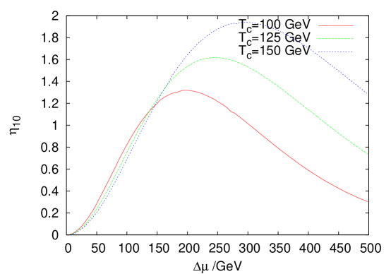
Figure 1: The dependence of $\eta_{10}\equiv 10^{10}\eta$ on the chargino mass parameter $\Delta\mu=\mu_{0}$. The parameters used are $l_{w}=10/T_{c}$ and $\Delta q_{s}=\pi/10$.

To give some feeling about the produced BAU, we note that a good estimate of the predicted $\eta_{10}$ is in this case given by the formula

$$\eta_{10}\approx\,c(T_{c})\,\,\frac{\Delta q_{s}}{\pi}\frac{1}{\,l_{w}\,T_{c}}\,\left(\frac{\mu_{0}}{\tau T_{c}}\right)^{\frac{3}{2}}\,\frac{\Delta\mu}{\tau T_{c}}\,\exp(-\mu_{0}/\tau T_{c}),$$ (26)

with $c(T_{c})\approx 1.6\,T_{c}/$GeV and $\tau\approx 0.78$. This formula characterizes the BAU in the case of large $M_{2}\approx 1$ TeV and $\mu_{0}\approx\Delta\mu$.

IV.2 EDM constraints in the nMSSM

The most severe experimental constraints on CP violation come from measurements of the EDM of the electron, $d_{e}<1.6\times 10^{-27}\,e\,{\rm cm}$ Regan:2002ta , and neutron, $d_{n}<3.0\times 10^{-26}\,e\,{\rm cm}$ Baker:2006ts . Already at the one-loop level, contributions of the superpartners give sizable effects in the case of CP-violating phases of $O(1)$. These one-loop diagrams are the same in the nMSSM and MSSM, setting $\mu=-\lambda\langle S\rangle$. Minimizing the Higgs potential, we can compute the phase of the effective $\mu$ parameter. Of course, this phase could be neutralized by introducing a compensating phase in the parameter $M_{2}$. Such a tuning would allow us to eliminate the one-loop EDMs completely, without much affecting the generated baryon asymmetry, since the dominating source is proportional to the change in the phase $\Delta q_{s}$ and not sensitive to the value of $q_{s}=\arg(\mu)$ in the broken phase. This is not possible in the MSSM, because there the produced BAU is, like the electron EDM contribution from the charginos, proportional to the combination ${\rm Im}(\mu M_{2})$.

However, here we take a different approach, using only the phase $q_{t}$ in the Higgs potential as sole source of CP violation. The one-loop EDMs then induce mass bounds for the first and second generation squarks and sleptons; depending on the model parameters these are in the range from a few TeV up to $50$ TeV Pospelov:2005pr . Since the constraints from the neutron EDM are usually less stringent than the ones coming from the electron EDMs, we will focus in the following on the latter. In single cases we also calculated the Barr–Zee type contributions to the neutron EDM Barr:1990vd , but they barely reach the most recent experimental bounds Baker:2006ts .

Besides heavy sfermion masses, there is another possibility to suppress the one-loop electron EDM in our model. Notice that the absolute value of the CP-violating phase $(q_{s}+q)$ can be smaller in the broken phase than in the symmetric phase. This phase $(q_{s}+q)$ is the only CP-odd combination that enters the electron EDMs on the one-loop level in our simplified nMSSM model, with CP violation only in the $t_{s}$ parameter. Hence, there is the possibility that today’s observed $\sin(q_{s}+q)\ll 1$, even though the phase $q_{s}$ greatly changed during the phase transition thus producing the BAU. We will analyze this possibility in detail in Sec. VI. The explicit form of the one-loop electron EDM contributions is given in Appendix B. This possibility entails a certain amount of tuning.

Additional EDMs can be generated from two-loop chargino or Higgs graphs (see, for instance, Pospelov:2005pr and references therein). Notice that the MSSM two-loop chargino contribution to the electron EDM Chang:2002ex ; Pilaftsis:2002fe is proportional to $\tan\beta$ and hence subleading in our model that usually predicts $\tan\beta\sim O(1)$. Potentially harmful diagrams, including the additional CP-odd scalar in the nMSSM, are small as well because of the modest $\tan\beta$ and because only the Higgs component of the CP-odd scalars couples to the charginos, while the singlet component delivers the additional CP violation (for a calculation of these contributions see Chang:1998uc ).

V Electroweak Phase Transition

One of the parameters entering our baryogenesis analysis is the thickness of the Higgs wall profile during the electroweak phase transition $l_{w}$. Since our CP-violating source is a second-order effect in gradients, the integrated BAU scales as $\eta\sim 1/l_{w}$, as already mentioned in Eq. (23).

To determine the wall thickness $l_{w}$ one has to examine the dynamics of the phase transition MooreProkopec:1995 . This has been done for the MSSM in Ref. Moreno:1998bq and for the NMSSM in Ref. Huber:2000mg . Typical values for the MSSM seem to be close to $l_{w}=10/T_{c}$. In the nMSSM, we expect rather thin wall profiles, since the linear singlet term and the trilinear singlet Higgs term in the effective potential will make the phase transition much stronger than the loop-suppressed stop corrections that are responsible for the first-order phase transition in the MSSM. In the light of Eq. (23) this will further enhance the produced asymmetry with respect to the MSSM case.

To determine the dynamical parameters of the wall, we solved for the classical bounce solution of the Higgs and singlet fields $(\phi_{1},\phi_{2},\phi_{s},q,q_{s})$ at the critical temperature (where the two minima of the potential are degenerate). Our numerical approach is based on the variation of the classical action and is discussed in detail in Ref. Konstandin:2006nd .

Another parameter relevant to the dominating source in Eq. (22) is the profile of the CP-violating phase of the singlet field. A typical solution is displayed in Fig. 2 corresponding to the parameters $\Delta q_{s}=0.119$ and $l_{w}=4.81\,T_{c}^{-1}$.

Figure 2: A typical wall profile for the parameter $q_{s}$, corresponding to the parameters $\Delta q_{s}=0.119$ and $l_{w}=4.81\,T_{c}^{-1}$.

To illuminate a little bit the nature of the phase transition, we will recall some approximate analytical criterion for the occurrence of a first-order phase transition, first given in a slightly different way in Ref. Menon:2004wv . Consider the tree-level potential in Eq. (6) without CP violation, $q_{t}=0$. Additionally assume that the temperature effects give rise to the effective potential

$$\Delta V^{T}=\alpha\,\phi^{2}T^{2},$$ (27)

where $\alpha$ is some unspecified positive constant. In Ref. Menon:2004wv it was shown that a necessary condition for a first-order phase transition is approximately given by

$$m_{s}^{2}<\frac{1}{\tilde{\lambda}}\left|\frac{\lambda^{2}t_{s}}{m_{s}}-m_{s}\tilde{a}\right|.$$ (28)

This can be seen in the following way. Given a certain value for $\phi$, $\phi_{s}$ can easily be evaluated to be

$$\phi_{s}=-\left(\frac{t_{s}+\tilde{a}\phi^{2}}{m_{s}^{2}+\lambda^{2}\phi^{2}}\right).$$ (29)

Using this in our potential, and expanding around $\phi=0$, we obtain

$$V+\Delta V^{T} = -\frac{t_{s}^{2}}{m_{s}^{2}}+\left(M^{2}+\alpha\,T^{2}\right)\phi^{2}+\tilde{\lambda}^{2}\,\phi^{4}-\frac{(t_{s}+\tilde{a}\phi^{2})^{2}}{m_{s}^{2}+\lambda^{2}\phi^{2}}$$ (30)

$$= c_{0}+c_{1}\phi^{2}+c_{2}\phi^{4}+c_{3}\phi^{6}\cdots,$$

with the coefficients

$$c_{0} = -\frac{t_{s}^{2}}{m_{s}^{2}},$$

$$c_{1} = M^{2}+\alpha\,T^{2}-\frac{2\tilde{a}t_{s}}{m_{s}^{2}}+\frac{\lambda^{2}t_{s}^{2}}{m_{s}^{4}},$$

$$c_{2} = \tilde{\lambda}^{2}-\frac{1}{m_{s}^{2}}\left(\tilde{a}-\frac{\lambda^{2}t_{s}}{m_{s}^{2}}\right)^{2},$$

$$c_{3} = \frac{\lambda^{2}}{m_{s}^{4}}\left(\tilde{a}-\frac{\lambda^{2}t_{s}}{m_{s}^{2}}\right)^{2}.$$ (31)

If the symmetric minimum is absent at zero temperature, $c_{1}(T=0)<0$, a temperature $T_{2}$ can be found, such that $c_{1}(T_{2})=0$. For this temperature there exists a lower-lying potential minimum in the case $c_{2}<0$, which is equivalent to the condition in Eq. (28). Since for temperatures $T\gtrsim T_{2}$ a potential well develops between the symmetric and the lower broken vacuum, a first-order phase transition is possible, given the vacuum decay rate is large enough such that the transition occurs before the temperature $T_{2}$ is reached. Hence, it is possible in the nMSSM to obtain a first-order phase transition due to tree-level dynamics, in contrast to the MSSM. Analyzing the numerical results, we will see that the constraint in Eq. (28) is usually fulfilled in viable models, even if the one-loop contributions to the potential and the CP phase are included and hence that the phase transition is dominated by the tree-level dynamics.

The argument just presented is a concrete realization of the general effective field theory approach recently discussed in Refs. GSW04 ; BFHS04 . There it was shown that a strong first-order phase transition can be induced at tree-level by the interplay of a negative $\phi^{4}$ term and a positive $\phi^{6}$ term which stabilizes the potential. The suppression scale of the $\phi^{6}$ term should be somewhat below a TeV for the mechanism to work. Here the relevant $\phi^{4}$ and $\phi^{6}$ operators are generated by integrating out the singlet field. This generalizes the usual situation, where the phase transition is induced by a negative $\phi^{3}$ term and a positive $\phi^{4}$ term.

VI Numerical Analysis

To inspect the parameter space of the nMSSM we proceed as follows. First, we choose random parameters for the Higgs potential in the ranges displayed in Tab. 2. To ensure maximal numerical stability, all chosen parameters are of $O$(1), and can be thought of as dimensionless parameters. Those parameters then lead not to the physical Higgs vev, but to some dimensionless Higgs vev $\phi_{0}$. Finally, all dimensionful quantities, such as the critical temperature or the mass spectrum have to be scaled with $(173.458$ GeV)/$\phi_{0}$ to yield the physical values. During the minimization of the potential, stable and metastable broken minima were analyzed. Depending on the parameters, metastable minima occur but, in the CP-conserving case $q_{t}=0$, no transitional (spontaneous) CP violation was observed in contrast to the NMSSM Huber:2000mg that contains an additional cubic singlet term.

Next, we correct the bare parameters with the one-loop contributions of Eq. (8) and confront them with the constraints on the mass spectrum from Tab. 1 and on the Z-width from Eq. (16).

lower bound		parameter		upper bound
0.1	$<$	$m_{1}$	$<$	1
0.1	$<$	$m_{2}$	$<$	1
0.1	$<$	$m_{12}$	$<$	2
0	$<$	$m_{s}$	$<$	2
$-2$	$<$	$\lambda$	$<$	2
0	$<$	$a_{\lambda}$	$<$	2
0	$<$	$t_{s}^{1/3}$	$<$	2
0	$<$	$q_{t}$	$<$	$2\,\pi$

Table 2: Dimensionless parameter ranges used for the numerical analysis.

If the parameter set passes these constraints, we add the temperature dependent contributions to the effective potential as explained in Sec. II.3 and examine the phase transition. We require that the models have a first-order phase transition of sufficient strength Menon:2004wv ; Shaposhnikov:1987pf , $\phi_{0}/T_{c}>0.9$.

Before we discuss baryogenesis in our model, we would like to examine restrictions on the parameters imposed by the constraints on the mass spectrum and comment on the criterion for a first-order phase transition given in the last section in Eq. (28).

First, the eight parameters given in Tab. 2 have to lead to the correct Higgs vev, which is achieved by a rescaling of the dimensionful parameters. Hence our parameter space is effectively only seven dimensional. One restriction on the parameters is that $a_{\lambda}$ cannot be chosen arbitrarily large, since this destabilizes the potential in the negative $\phi_{s}$ direction. Analyzing the parameter sets that fulfill the mass constraints, one observes that the parameters $\lambda$ and $q_{t}$ are not distributed homogeneously. Small values of $\lambda$ make it seemingly difficult to fulfill the mass bound of the chargino, since one of the diagonal entries of the chargino mass matrix is $-\lambda\phi_{s}$. To have a potential with extremely large vev $\phi_{s}$ requires at least some fine-tuning, since the one-loop contribution tends to yield an effective potential that is unbounded from below, if the tree-level parameters are chosen to provide a large vev $\phi_{s}$. Large values of $\lambda$ hence seem to be the more natural choice, even though they can lead to a Landau pole Menon:2004wv . Usually, the mass constraints on the neutralinos are automatically fulfilled, if the charginos surpass their more restrictive bounds, but additional constraints on the parameters enter through the spectrum of the Higgs particles. In many cases, a range of values for the parameter $a_{\lambda}$ can be found, where off-diagonal elements in the Higgs mass matrix cancel, which tends to enlarge the lightest Higgs mass. In addition the parameter $a_{\lambda}$ has a strong influence on the phase transition according to Eq. (28).

This situation is demonstrated in Fig. 3 for a parameter set with a rather small parameter $\lambda$. The parameters $m_{1},m_{2},m_{12},m_{s}$ are chosen such that $\tan(\beta)=2.0$, $\phi_{s}=-250$ GeV, $\phi=173$ GeV and $M_{a}=500$ GeV at the tree-level, where the CP-odd Higgs mass parameter is defined by

$$M_{a}^{2}=\frac{1}{\sin{\beta}\cos{\beta}}\left(m^{2}_{12}-a_{\lambda}\phi_{s}\right).$$ (32)

The remaining parameters are $\lambda=0.55$, $t_{s}^{1/3}=70$ GeV, $q_{s}=0.3$, while $a_{\lambda}$ is varied. For $172$ GeV $<a_{\lambda}<178$ GeV, this model develops a strong first-order phase transition and generates more than the observed BAU. For lower values of $a_{\lambda}$, the model has no stable broken phase, while for larger values of $a_{\lambda}$, the phase transition is too weak. The plotted Higgs mass is that of the third lightest Higgs, but the two lighter states would have escaped detection at LEP because of the suppressed coupling to the $Z$-boson. This example demonstrates that even though there exist viable models without Landau pole in $\lambda$, this possibility entails a certain amount of tuning.

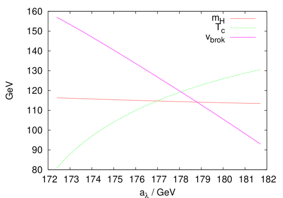
Figure 3: The critical temperature $T_{c}$, the Higgs vev $\phi$ in the broken phase at $T_{c}$ and one Higgs mass as functions of $a_{\lambda}$.

The second parameter that is restricted by the mass constraints is the CP-violating phase $q_{t}$. The reason for this effect is that values with $\cos(q_{t})\approx-1$ lead to smaller Higgs masses. Fig. 4 displays the parameters $\lambda$ and $q_{t}$ for a set of random models that fulfill the mass constraints.

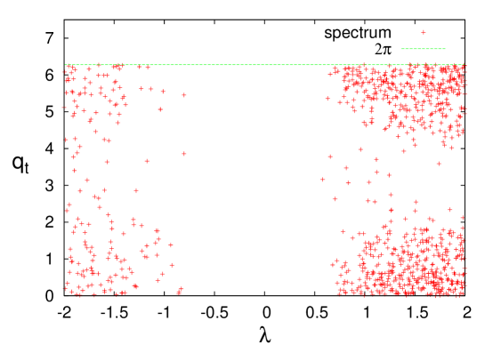
Figure 4: The parameters $\lambda$ and $q_{t}$ for a set of random models that fulfill the mass constraints.

Demanding a strong first-order phase transition further restricts the parameter space. In Fig. 5 we plot the left-hand side versus the right-hand side of the criterion in Eq. (28) (both sides are scaled by $1/(m_{1}m_{2})$ to make them dimensionless). In the left plot we use random models that fulfill the mass constraints on the spectrum, but are unconstrained otherwise; in the right plot we impose the mass constraints on the model and require a strong first-order phase transition. In the latter case, most of the parameter sets are in accordance with Eq. (28), while the parameter sets in the former case are evenly distributed. Hence, the tree-level criterion for the phase transition seems to be applicable even if the one-loop contributions to the effective potential and the CP phase are taken into account.

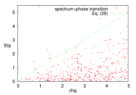
Figure 5: The plots show the combinations of the parameters that enter the tree-level condition for a first-order phase transition, Eq. (28). The left plot contains parameter sets that fulfill only the mass constraints, while the right plot contains parameter sets that have in addition a strong first-order phase transition.

In the nMSSM, for several reasons, we expect a much larger BAU than in the MSSM. First, the parameter $\tan(\beta)$, which needs to be large in the MSSM, is naturally $O(1)$ in the nMSSM as depicted in Fig. 6. This does not only help to suppress the two-loop contributions to the EDMs, as discussed in the previous section, but also enhances the contributions from the source in Eq. (21).

Figure 6: The binned result of the parameter $\tan(\beta)$ for the parameter sets with a strong first-order phase transition.

Secondly, the wall thickness, which in the MSSM usually is of order $20/T_{c}$–$30/T_{c}$ Moreno:1998bq , can be much smaller, since the phase transition is strengthened by the linear and trilinear terms in the effective potential. This claim is supported by Fig. 7.

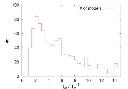
Figure 7: The binned result of the parameter $l_{w}$ for the parameter sets with a strong first-order phase transition.

The third reason for the enhancement of the BAU in the nMSSM with respect to the MSSM is the additional source in Eq. (22), which is in many cases dominating the generation of the BAU.

Finally, we calculate the generated baryon asymmetry and compare the result with the experimental observation, $\eta=(0.87\pm 0.03)\times 10^{-10}$ eta . The result is shown in Figs. 8 and 9. Approximately 50% of the parameter sets predict a higher value than the observed baryon asymmetry in the model with large $M_{2}=1$ TeV, while this number increases to 63% for small $M_{2}=200$ GeV.

Figure 8: The binned result for the BAU analysis for large $M_{2}=1$ TeV. Approximately 50% of the parameter sets predict a value of the baryon asymmetry higher than the observed one. The bottom line corresponds to parameter sets that fulfill current bounds at the electron EDM with 1 TeV sfermions (4.8%).

Figure 9: The binned result for the BAU analysis for small $M_{2}=200$ GeV. Approximately 63% of the parameter sets predict a value of the baryon asymmetry higher than the observed one. The bottom line corresponds to models that fulfill current bounds at the electron EDM with 1 TeV sfermions (6.2%).

In addition, we plotted the BAU generated by parameter sets that fulfill the experimental bounds on the electron EDM with sfermion masses of 1 TeV in the first and second generation. Some of them predict a BAU in accordance with observation, and hence give the possibility to construct nMSSM models that contain less constrained sfermions (lighter than 1 TeV) being at the same time consistent with EDM constraints and baryogenesis. In some cases the electron EDM is small because of a random cancellation between the neutralino and chargino contributions, but occasionally the suppression of the electron EDM is due to the fact that the combination $\sin(q_{s}+q)$ is relatively small in the broken phase.

VII Conclusion

We have analyzed the phase transition and baryogenesis in the nMSSM (1) – (II.1) with CP violation in the singlet sector. We have shown that the singlet field enhances the strength of the phase transition in such a way that one typically obtains a strong phase transition, as required for successful baryogenesis. This is to be contrasted with the MSSM, in which the mass of the lightest Higgs field must not be greater than about $120~{}{\rm GeV}$, and the right-handed stop must be light, $m_{\tilde{t}_{R}}\in\left(120,160\right)~{}{\rm GeV}$.

Next we performed the calculation of baryogenesis mediated by charginos in the nMSSM. After calculating the CP-violating sources in the gradient expansion, we argued that in most of the parameter space the dominant source comes from the second-order semiclassical force in the Boltzmann transport equation for charginos. The source related to flavor mixing, of first order in the gradient expansion, tends to be smaller, because the bubble wall is rather thin. For a generic choice of parameters, one is far from the chargino mass degeneracy, where the first-order source may be important. To come to this conclusion, we used an approach to the calculation of the first-order sources kps ; kpss that differs from earlier work Menon:2004wv ; cmqsw ; cmqsw2 in the sense that our treatment of sources is basis independent, and the magnitude of the source in the transport equation is unambiguous. Using this advanced transport theory, the first-order sources are of a somewhat lower amplitude and exhibit a much narrower resonance near the chargino mass degeneracy, with the effect that in most of the parameter space the second-order source dominates. In the MSSM, this is not the case for the chargino-mediated baryogenesis because the wall tends to be thicker, thus weakening the second-order (semiclassical force) source, while leaving the first-order source more or less unchanged. Furthermore, the dominant second-order source of baryogenesis in the nMSSM, Eq. (22), is not present in the MSSM. Owing to these differences, successful baryogenesis in the MSSM is only possible near the resonance (chargino mass degeneracy), and with nearly maximum CP violation, which is in conflict with the current EDM bounds, unless a tuning of parameters is invoked kpss .

On the other hand our analysis of the baryon production in the nMSSM looks promising. When we restrict the CP-violating phase in the singlet sector to be about $q_{t}\sim 0.3$, and take $\tan(\beta)\sim 1$, we still get baryon production consistent with the observed value. This choice certainly does not violate any of the current EDM bounds. When $q_{t}$ is chosen randomly, approximately $50\%$ ($63\%$) models predict more than the observed BAU when $M_{2}=1~{}{\rm TeV}$ ($M_{2}=200~{}{\rm GeV}$), which indicates that baryogenesis in the nMSSM is generic.

It is finally interesting to compare baryogenesis in the nMSSM and in the general NMSSM formerly analyzed in Ref. Huber:2000mg . Because of the presence of a singlet self coupling and an explicit $\mu$ term, the NMSSM allows for a much richer Higgs phenomenology. (However, some additional assumptions about the structure of the higher dimensional operators have to be made, in order to prevent the destabilization of the electroweak scale by corrections to the singlet tadpole.) There is no danger of a light singlino state, so that the model can account for the observed baryon asymmetry also for values of $\lambda\lesssim 0.1$ and large $\tan\beta$. It also allows for transitional CP violation, which means an electroweak phase transition that connects a high-temperature CP-broken phase with a low-temperature CP-symmetric phase. This way there are varying complex phases in the bubble wall, without leaving a trace at low temperatures. In the present model this possibility is prevented by the strongly constrained Higgs potential.

In Ref. Huber:2000mg the source terms were computed by solving the Dirac equation for the charginos in the WKB approximation. As has been recently shown in Ref. FH06 , this formalism can reproduce the second-order source of Ref. Kainulainen:2001cn , used in the present work, if the Lorentz transformation to a general Lorentz frame is done carefully (see also Ref. Kainulainen:2002th ). These results suggest that in Ref. Huber:2000mg the baryon asymmetry was underestimated by a factor of 2 to 5. It seems to be interesting to update this analysis to meet the present experimental constraints. It also seems promising to apply the presented techniques to more general supersymmetric models, such as models with extra U(1) symmetries Kang:2004pp .

Appendix A Mass Spectrum of the nMSSM

In the following we collect the mass matrices that have been used in the one-loop potentials in Sec. II.

We used the physical constants

$$\sin(\theta_{W})=0.2312, \quad\alpha_{EW}=1/127.907,$$ (33)

$$m_{Z}=91.1876\textrm{ GeV}, \quad m_{t}=165.0\textrm{ GeV},$$ (34)

which give rise to the values

$$g=0.357,\quad g^{\prime}=0.652,\quad\phi_{0}=173.458\textrm{ GeV},$$ (35)

where $\phi_{0}$ denotes the $T=0$ value of the vev $\phi$.

If not stated differently, we have used the SUSY-breaking parameters

$$m_{U}=m_{Q}=500\textrm{ GeV}, \quad a_{t}=100\textrm{ GeV},\quad$$

$$M_{2}=2M_{1}=200\textrm{ GeV}, \quad m_{E}=500\textrm{ GeV},$$ (36)

which enter in the mass matrices that we will define subsequently.

A.1 Higgs bosons

For the neutral Higgs bosons we use the notation

$$H^{0}_{i}=\textrm{e}^{iq_{i}}(\phi_{i}+S_{i}+iP_{i}),\quad S=\textrm{e}^{iq_{s}}(\phi_{s}+S_{s}+iP_{s}),$$ (37)

and $q_{1}=q_{2}=q/2$. The corresponding mass matrix has the following form

$$M_{H}^{2}=\begin{pmatrix}M^{2}_{SS}&M^{2}_{SP}\\ M^{2}_{PS}&M^{2}_{PP}\end{pmatrix},$$ (38)

with the matrices $M_{SS}$, $M_{SP}=M_{PS}^{\dagger}$, and $M_{PP}$ given by the following entries. The CP-even entries at the tree-level read

$$M^{2}_{SS11} = m_{1}^{2}+\lambda^{2}(\phi_{2}^{2}+\phi_{s}^{2})+\frac{\bar{g}^{2}}{4}(3\phi_{1}^{2}-\phi_{2}^{2}),$$

$$M^{2}_{SS12} = -m_{12}^{2}\cos(q)+a_{\lambda}\phi_{s}\cos(q+q_{s})+\frac{1}{2}\phi_{1}\phi_{2}(4\lambda^{2}-\bar{g}^{2}),$$

$$M^{2}_{SS13} = a_{\lambda}\phi_{2}\cos(q+q_{s})+2\lambda^{2}\phi_{1}\phi_{s},$$

$$M^{2}_{SS22} = m_{2}^{2}+\lambda^{2}(\phi_{1}^{2}+\phi_{s}^{2})+\frac{\bar{g}^{2}}{4}(3\phi_{2}^{2}-\phi_{1}^{2}),$$

$$M^{2}_{SS23} = a_{\lambda}\phi_{1}\cos(q+q_{s})+2\lambda^{2}\phi_{2}\phi_{s},$$

$$M^{2}_{SS33} = m_{s}^{2}+\lambda^{2}\phi^{2}.$$ (39)

The CP-odd entries are

$$M^{2}_{PP11} = m_{1}^{2}+\lambda^{2}(\phi_{2}^{2}+\phi_{s}^{2})+\frac{\bar{g}^{2}}{4}(\phi_{1}^{2}-\phi_{2}^{2}),$$

$$M^{2}_{PP12} = m_{12}^{2}\cos(q)-a_{\lambda}\phi_{s}\cos(q+q_{s}),$$

$$M^{2}_{PP13} = -a_{\lambda}\phi_{2}\cos(q+q_{s}),$$

$$M^{2}_{PP22} = m_{2}^{2}+\lambda^{2}(\phi_{1}^{2}+\phi_{s}^{2})+\frac{\bar{g}^{2}}{4}(\phi_{2}^{2}-\phi_{1}^{2}),$$

$$M^{2}_{PP23} = -a_{\lambda}\phi_{1}\cos(q+q_{s}),$$

$$M^{2}_{PP33} = m_{s}^{2}+\lambda^{2}\phi^{2}.$$ (40)

Finally the CP-mixed entries yield

$$M^{2}_{SP12} = m_{12}^{2}\sin(q)-a_{\lambda}\phi_{s}\sin(q+q_{s}),$$

$$M^{2}_{SP13} = -a_{\lambda}\phi_{2}\sin(q+q_{s}),$$

$$M^{2}_{SP23} = -a_{\lambda}\phi_{1}\sin(q+q_{s}).$$ (41)

In the CP-conserving case the submatrix (41) vanishes so that CP-even and CP-odd states do not mix.

If the one-loop effective potential is included, we determine the masses of the neutral Higgses by the second derivatives of the effective potential.

The mass matrix of the charged Higgs bosons in the basis $(H_{1}^{-},\bar{H}_{2}^{+})$ contains the complex entries

$$M^{2}_{H^{\pm}_{11}} = m_{1}^{2}+\lambda^{2}\phi-\frac{\bar{g}^{2}}{4}(\phi_{2}^{2}-\phi_{1}^{2})+\frac{g^{2}}{2}\phi_{2}^{2},$$

$$M^{2}_{H^{\pm}_{12}} = -\frac{1}{2}\phi_{1}\phi_{2}(2\lambda^{2}-g^{2})+m^{2}_{12}\textrm{e}^{iq}-a_{\lambda}\phi_{s}\textrm{e}^{i(q+q_{s})},$$

$$M^{2}_{H^{\pm}_{22}} = m_{2}^{2}+\lambda^{2}\phi-\frac{\bar{g}^{2}}{4}(\phi_{1}^{2}-\phi_{2}^{2})+\frac{g^{2}}{2}\phi_{1}^{2}.$$ (42)

A.2 Charginos and Neutralinos

The chargino mass matrix reads

$$M_{\tilde{\chi}^{\pm}}=\begin{pmatrix}0&Y_{\tilde{\chi}^{\pm}}^{T}\\ Y_{\tilde{\chi}^{\pm}}&0\\ \end{pmatrix},\quad Y_{\tilde{\chi}^{\pm}}=\begin{pmatrix}M_{2}&g\phi_{2}\textrm{e}^{-i\frac{q}{2}}\\ g\phi_{1}\textrm{e}^{-i\frac{q}{2}}&-\lambda\phi_{s}\textrm{e}^{iq_{s}}\\ \end{pmatrix},$$ (43)

and is diagonalized by the biunitary transformation $Y^{\rm diag}_{\tilde{\chi}^{\pm}}=U^{*}Y_{\tilde{\chi}^{\pm}}V^{\dagger}$.

The symmetric mass matrix of the neutralinos in the basis $\tilde{\chi}^{0}=(i\tilde{B},i\tilde{W}^{3},\tilde{H}_{1}^{0},\tilde{H}_{2}^{0},\tilde{S})$ yields

$$M_{\tilde{\chi}^{0}}=\begin{pmatrix}M_{1}&.&.&.&.\\ 0&M_{2}&.&.&.\\ -\frac{g^{\prime}}{\sqrt{2}}\phi_{1}\textrm{e}^{-i\frac{q}{2}}&\frac{g}{\sqrt{2}}\phi_{1}\textrm{e}^{-i\frac{q}{2}}&0&.&.\\ \frac{g^{\prime}}{\sqrt{2}}\phi_{2}\textrm{e}^{-i\frac{q}{2}}&-\frac{g}{\sqrt{2}}\phi_{2}\textrm{e}^{-i\frac{q}{2}}&\lambda\phi_{s}\textrm{e}^{iq_{s}}&0&.\\ 0&0&\lambda\phi_{2}\textrm{e}^{i\frac{q}{2}}&\lambda\phi_{1}\textrm{e}^{i\frac{q}{2}}&0\end{pmatrix},$$ (44)

and can be diagonalized using a unitary matrix, $M^{\rm diag}_{\tilde{\chi}^{0}}=X^{T}M_{\tilde{\chi}^{0}}X$.

A.3 Gauge bosons

The mass of the $W$-boson is given by

$$m^{2}_{W}=\frac{1}{2}g^{2}\phi^{2},$$ (45)

while the photon and the $Z$-boson share the following hermitian mass matrix

$$M^{2}_{Z\gamma}=\begin{pmatrix}\frac{1}{2}g^{2}\phi^{2}&-\frac{1}{2}gg^{\prime}\phi^{2}\\ -\frac{1}{2}gg^{\prime}\phi^{2}&\frac{1}{2}{g^{\prime}}^{2}\phi^{2}\end{pmatrix}$$ (46)

that leads to the $Z$-boson mass $m_{Z}=({\bar{g}}/{\sqrt{2}})\phi$.

A.4 Tops and stops

The top quark has the mass

$$m^{2}_{t}=y_{t}^{2}\phi_{2}^{2},$$ (47)

and the masses of the stops are given by the following hermitian matrix

$$M^{2}_{\tilde{t}}=\begin{pmatrix}m_{Q}^{2}+m_{t}^{2}+\frac{1}{4}(g^{2}-\frac{1}{3}{g^{\prime}}^{2})(\phi_{1}^{2}-\phi_{2}^{2})&a_{t}\phi_{2}\textrm{e}^{iq/2}+y_{t}\lambda\phi_{s}\phi_{1}\textrm{e}^{-i(q_{s}+q/2)}\\ a_{t}\phi_{2}\textrm{e}^{-iq/2}+y_{t}\lambda\phi_{s}\phi_{1}\textrm{e}^{i(q_{s}+q/2)}&m_{U}^{2}+m_{t}^{2}+\frac{1}{3}{g^{\prime}}^{2}(\phi_{1}^{2}-\phi_{2}^{2})\end{pmatrix}.$$ (48)

A.5 Sneutrinos and selectrons

For the selectrons we have

$$M^{2}_{\tilde{e}}=\begin{pmatrix}m_{E}&-\lambda\phi_{s}e^{iq_{s}}m_{e}\,\tan(\beta)\\ -\lambda\phi_{s}e^{-iq_{s}}m_{e}\,\tan(\beta)&m_{E}\end{pmatrix},$$ (49)

that is diagonalized via the transformation $M^{2}_{\tilde{e},\rm diag}=D^{\dagger}M^{2}_{\tilde{e}}D$.

For the electron EDM contributions from the charginos we use a sneutrino of mass $m_{\tilde{\nu}}=1$ TeV.

Appendix B One-loop Contributions to the Electron EDM

In this Appendix we briefly discuss the one-loop contributions to the electron EDM coming from chargino and neutralino exchange. For the sfermions of the first two generations we assume masses of 1 TeV. The contribution from the charginos is given by Ibrahim:1998je :

$$\frac{d_{\rm e-chargino}}{e}=\frac{\alpha_{EM}}{4\pi\sin^{2}(\theta_{W})}\sum_{i=1}^{2}\frac{m_{\tilde{\chi}_{i}^{+}}}{m^{2}_{\tilde{\nu}_{e}}}\textrm{ Im}(\Gamma_{ei})\textrm{ A}\bigg{(}\frac{m^{2}_{\tilde{\chi}_{i}^{+}}}{m^{2}_{\tilde{\nu}_{e}}}\bigg{)},$$ (50)

where

$$\Gamma_{ei}=\kappa_{e}U^{*}_{i2}V_{i1},\quad\kappa_{e}=\frac{m_{e}\,e^{iq/2}}{\sqrt{2}m_{W}\cos(\beta)}.$$ (51)

Here, the matrices $U$ and $V$ diagonalize the chargino mass matrix as defined in the previous section and

$$\textrm{ A}(r)=\frac{1}{2(1-r)^{2}}\left(3-r+\frac{2}{1-r}\ln(r)\right)$$ (52)

denotes the loop function.

Analogously, the contribution from the neutralinos is Ibrahim:1998je ; delAguila:1983kc

$$d_{\rm e-neutralino}/e=\frac{\alpha_{EM}}{4\pi\sin^{2}(\theta_{W})}\sum_{k=1}^{2}\sum_{i=1}^{4}\frac{m_{\tilde{\chi}_{i}^{0}}}{m^{2}_{\tilde{e}}}\textrm{ Im}(\eta_{eik})\textrm{ B}(m^{2}_{\tilde{\chi}_{i}^{0}}/m^{2}_{\tilde{e}}),$$ (53)

with

$$\eta_{eik} = \left[(\tan(\theta_{W})X_{1i}+X_{1i})D_{1k}^{*}+\sqrt{2}\kappa_{e}X_{3i}D_{2k}^{*}\right]$$ (54)

$$\times\left[\tan(\theta_{W})X_{1i}D_{2k}^{*}+\frac{\kappa_{e}}{\sqrt{2}}X_{3i}D_{1k}^{*}\right].$$

In this equation, $X$ and $D$ diagonalize the neutralinos and selectrons, respectively. The loop function B is defined by

$$\textrm{ B}(r)=\frac{1}{2(1-r)^{2}}\left(1+r+\frac{2r}{1-r}\ln(r)\right).$$ (55)

Following the discussion in Ref. Ibrahim:1998je , it can be shown that if $q_{t}$ is the only CP-violating phase in the Higgs sector, both contributions depend only on the CP-odd combination $(q_{s}+q)$. The current experimental bound on the electron EDM is $d_{e}<1.6\times 10^{-27}\,e\,{\rm cm}$  Regan:2002ta .

Appendix C Example sets

In this appendix we give some examples of parameters that develop a strong first-order phase transition. The examples are not chosen arbitrarily, but they represent specific cases. The first set, shown in Tables 5–10, accomplishes the generation of a large BAU thanks to a relatively thin wall. On the other hand the electron EDM is extremely small, partly because the combination $q+q_{s}$ is rather small in the broken phase and partly due to a coincidental cancellation between the neutralino and the chargino contributions to the electron EDM. Set number 6 describes a model with small $\lambda$, taken from Fig. 3 with $a_{\lambda}=177.3$ GeV. This model generates more than the observed BAU, but the calculated electron EDM is slightly too big, so that the sfermions of the first two generations have to be heavier than 1 TeV. Starting from $q_{t}~{}\sim 0.1$ instead of 0.3 should yield $\eta_{10}\sim 1$ and an electron EDM within the experimental bound. The remaining sets are randomly chosen. Set number 6 demonstrates that even a sizable value of $q_{t}$ does not lead to a large baryon asymmetry if $\Delta q_{s}$ is small along the bubble wall. The rather thick wall induces an additional suppression of $\eta_{10}$ in this case.

set	$m_{1}$ in GeV	$m_{2}$ in GeV	$m_{12}$ in GeV	$m_{s}$ in GeV	$\lambda$	$a_{\lambda}$ in GeV	$t_{s}^{1/3}$ in GeV	$q_{t}$
1	157.2	93.0	170.6	55.8	1.2642	268.2	98.4	2.113
2	124.2	149.2	215.0	127.2	1.4320	254.1	152.2	5.050
3	248.9	230.8	243.3	160.5	-0.8937	214.2	190.5	0.046
4	397.1	251.9	375.5	342.1	-1.2991	292.0	310.5	0.282
5	66.4	98.5	111.8	65.5	0.7656	95.3	102.0	6.193
6	425.1	165.7	240.1	26.8	0.5500	177.3	70.9	0.300

Table 3: Parameter examples used for the numerical analysis.

set	$\tilde{\chi}^{\pm}$		$H^{\pm}$	$\tilde{t}_{1/2}$
1	221.77	107.40	219.56	521.43	529.30
2	221.64	131.22	236.41	537.16	514.91
3	270.45	109.31	410.84	485.74	563.03
4	146.21	315.37	588.45	479.29	567.75
5	221.06	105.94	148.97	530.64	521.67
6	225.24	144.62	494.87	520.50	528.89

Table 4: The mass spectrum of the charginos, charged Higgses and stops (in GeV).

set	$S$, $P$
1	142.72	210.53	217.41	273.78	357.83
2	177.85	260.59	292.50	296.78	396.55
3	119.12	202.13	251.16	432.44	455.77
4	121.65	395.09	448.97	602.98	641.00
5	115.07	118.67	169.87	211.08	237.02
6	76.74	89.86	114.76	504.68	506.91

Table 5: The mass spectrum of the neutral Higgses (in GeV).

set	$\tilde{\chi}^{0}$
1	267.76	105.80	113.09	221.89	184.03
2	313.48	105.14	138.79	222.79	198.12
3	135.40	68.73	89.48	275.43	269.04
4	389.60	323.06	81.50	161.87	123.56
5	222.16	181.83	116.61	107.33	94.72
6	227.33	42.25	105.37	165.39	175.04

Table 6: The mass spectrum of the neutralinos (in GeV).

set	$\phi$ in GeV	$\beta$	$q$	$\phi_{s}$ in GeV	$q_{s}$
1	173.46	0.926	0.157	-71.0	-0.392
2	173.46	0.739	-0.214	-81.8	0.687
3	173.46	0.808	0.015	-202.9	-0.036
4	173.46	0.915	0.074	-202.6	-0.256
5	173.46	0.714	-0.024	-112.6	0.051
6	173.46	1.108	0.029	-251.9	-0.067

Table 7: The vevs in the broken phase at temperature $T=0$.

set	$\phi$ in GeV	$\beta$	$q$	$\phi_{s}$ in GeV	$q_{s}$
1	165.4	0.900	0.175	-71.4	-0.437
2	170.0	0.726	-0.223	-83.2	0.708
3	150.3	0.803	0.016	-214.9	-0.038
4	164.5	0.911	0.076	-207.4	-0.259
5	151.6	0.687	-0.029	-120.2	0.058
6	141.9	1.102	0.041	-261.5	-0.092

Table 8: The vevs in the broken phase at temperature $T=T_{c}$.

set	$\phi$ in GeV	$\beta$	$q$	$\phi_{s}$ in GeV	$q_{s}$
1	0.0	-	-	-281.4	-2.113
2	0.0	-	-	-241.6	1.233
3	0.0	-	-	-283.3	-0.046
4	0.0	-	-	-259.9	-0.282
5	0.0	-	-	-266.0	0.090
6	0.0	-	-	-471.5	-0.300

Table 9: The vevs in the symmetric phase at temperature $T=T_{c}$.

set	$T_{c}$ in GeV	$d_{e}$ in $10^{-27}\,e\,cm\,$	$l_{w}$ in $T_{c}^{-1}$	$\eta_{10}$
1	113.5	0.002	2.43	29.443
2	99.1	0.796	6.38	-3.214
3	109.1	0.499	7.82	0.014
4	78.6	5.894	34.01	0.005
5	115.8	-0.893	3.05	-0.398
6	105.6	-2.054	2.39	2.717

Table 10: The parameters of the phase transition and the generated BAU.

References

- (1) V. A. Kuzmin, V. A. Rubakov and M. E. Shaposhnikov, “On the anomalous electroweak baryon number nonconservation in the early universe”, Phys. Lett. B 155 (1985) 36.
- (2) A. G. Cohen, D. B. Kaplan and A. E. Nelson, “Diffusion enhances spontaneous electroweak baryogenesis”, Phys. Lett. B 336 (1994) 41 [hep-ph/9406345].
- (3) M. Joyce, T. Prokopec and N. Turok, “Electroweak baryogenesis from a classical force”, Phys. Rev. Lett. 75 (1995) 1695 [Erratum ibid. 75 (1995) 3375] [hep-ph/9408339]. M. Joyce, T. Prokopec and N. Turok, “Nonlocal electroweak baryogenesis. Part 2: the classical regime”, Phys. Rev. D 53 (1996) 2958 [hep-ph/9410282].
- (4) J.M. Cline, M. Joyce and K. Kainulainen, “Supersymmetric electroweak baryogenesis in the WKB approximation”, Phys. Lett. B417 (1998) 79, Erratum ibid. B448 (1999) 321 [hep-ph/9708393]. J. M. Cline, M. Joyce and K. Kainulainen, “Supersymmetric electroweak baryogenesis”, JHEP 0007 (2000) 018 [hep-ph/0006119]. J. M. Cline, M. Joyce and K. Kainulainen, “Supersymmetric electroweak baryogenesis. (Erratum)”, hep-ph/0110031.
- (5) K. Kainulainen, T. Prokopec, M. G. Schmidt and S. Weinstock, “First principle derivation of semiclassical force for electroweak baryogenesis”, JHEP 0106 (2001) 031 [hep-ph/0105295]. T. Prokopec, M. G. Schmidt and S. Weinstock, “Transport equations for chiral fermions to order h-bar and electroweak baryogenesis”, Ann. Phys. 314 (2004) 208 [hep-ph/0312110]. T. Prokopec, M. G. Schmidt and S. Weinstock, “Transport equations for chiral fermions to order h-bar and electroweak baryogenesis. II”, Ann. Phys. 314 (2004) 267 [hep-ph/0406140].
- (6) T. Konstandin, T. Prokopec, M. G. Schmidt and M. Seco, “MSSM electroweak baryogenesis and flavour mixing in transport equations”, Nucl. Phys. B 738 (2006) 1 [hep-ph/0505103].
- (7) M. Carena, M. Quiros, M. Seco and C. E. M. Wagner, “Improved results in supersymmetric electroweak baryogenesis”, Nucl. Phys. B 650 (2003) 24 [hep-ph/0208043].
- (8) M. Carena, J. M. Moreno, M. Quiros, M. Seco and C. E. M. Wagner, “Supersymmetric CP-violating currents and electroweak baryogenesis”, Nucl. Phys. B 599 (2001) 158 [hep-ph/0011055].
- (9) T. Konstandin, T. Prokopec and M. G. Schmidt, “Kinetic description of fermion flavor mixing and CP-violating sources for baryogenesis”, Nucl. Phys. B 716 (2005) 373 [hep-ph/0410135].
- (10) M. Joyce, K. Kainulainen and T. Prokopec, “The semiclassical propagator in field theory”, Phys. Lett. B 468 (1999) 128 [hep-ph/9906411].
- (11) L. Fromme and S.J. Huber, “Top transport in electroweak baryogenesis”, hep-ph/0604159.
- (12) J. M. Moreno, M. Quiros and M. Seco, “Bubbles in the supersymmetric standard model”, Nucl. Phys. B 526, 489 (1998) [hep-ph/9801272].
- (13) C. Panagiotakopoulos and K. Tamvakis, “Stabilized NMSSM without domain walls”, Phys. Lett. B446 (1999) 224 [hep-ph/9809475].
- (14) C. Panagiotakopoulos and K. Tamvakis, “New minimal extension of MSSM”, Phys. Lett. B469 (1999) 145 [hep-ph/9908351].
- (15) C. Panagiotakopoulos and A. Pilaftsis, “Higgs scalars in the minimal non-minimal supersymmetric standard model”, Phys. Rev. D 63 (2001) 055003 [hep-ph/0008268].
- (16) A. Dedes, C. Hugonie, S. Moretti and K. Tamvakis, “Phenomenology of a new minimal supersymmetric extension of the standard model”, Phys. Rev. D63 (2001) 055009 [hep-ph/0009125].
- (17) S.A. Abel, S. Sarkar and P.L. White, “On the cosmological domain wall problem for the minimally extended supersymmetric standard model”, Nucl. Phys. B454 (1995) 663 [hep-ph/9506359].
- (18) A. Menon, D. E. Morrissey and C. E. M. Wagner, “Electroweak baryogenesis and dark matter in the nMSSM”, Phys. Rev. D 70 (2004) 035005 [hep-ph/0404184].
- (19) D. Chang, W. F. Chang and W. Y. Keung, “New constraint from electric dipole moments on chargino baryogenesis in MSSM”, Phys. Rev. D 66 (2002) 116008 [hep-ph/0205084].
- (20) A. Pilaftsis, “Higgs-mediated electric dipole moments in the MSSM: an application to baryogenesis and Higgs searches”, Nucl. Phys. B 644, (2002) 263 [hep-ph/0207277].
- (21) M. Pietroni, “The electroweak phase transition in a nonminimal supersymmetric model”, Nucl. Phys. B402 (1993) 27 [hep-ph/9207227].
- (22) A.T. Davies, C.D. Froggatt and R.G. Moorhouse, “Electroweak baryogenesis in the next-to-minimal supersymmetric model”, Phys. Lett. B372 (1996) 88 [hep-ph/9603388].
- (23) S.J. Huber and M.G. Schmidt, “SUSY variants of the electroweak phase transition”, Eur. Phys. J. C10 (1999) 473 [hep-ph/9809506].
- (24) M. Bastero-Gil, C. Hugonie, S.F. King, D.P. Roy and S. Vempati, “Does LEP prefer the NMSSM?”, Phys. Lett. B489 (2000) 359 [hep-ph/0006198].
- (25) J. Kang, P. Langacker and T. Li, “Electroweak baryogenesis in a supersymmetric U(1)-prime model”, Phys. Rev. Lett. 94 (2005) 061801 [hep-ph/0402086].
- (26) S. J. Huber and M. G. Schmidt, “Electroweak baryogenesis: concrete in a SUSY model with a gauge singlet”, Nucl. Phys. B 606 (2001) 183 [hep-ph/0003122]. S. J. Huber, P. John, M. Laine and M. G. Schmidt, “CP violating bubble wall profiles”, Phys. Lett. B 475 (2000) 104 [hep-ph/9912278].
- (27) K. Funakubo, S. Tao and F. Toyoda, “Phase transitions in the NMSSM”, Prog. Theor. Phys. 114 (2005) 369 [hep-ph/0501052].
- (28) D. Bodeker, P. John, M. Laine and M. G. Schmidt, “The 2-loop MSSM finite temperature effective potential with stop condensation”, Nucl. Phys. B 497, (1997) 387 [hep-ph/9612364].
- (29) M. Laine and K. Rummukainen, “Two Higgs doublet dynamics at the electroweak phase transition: a non-perturbative study,” Nucl. Phys. B 597, (2001) 23 [hep-lat/0009025].
- (30) LEP Collaborations, ALEPH Collaboration, DELPHI Collaboration, L3 Collaboration, OPAL Collaboration and Line Shape Sub-Group of the LEP Electroweak Working Group, “Combination procedure for the precise determination of Z boson parameters from results of the LEP experiments”, hep-ex/0101027.
- (31) R. Harnik, G.D. Kribs, D.T. Larson and H.Murayama, “The minimal supersymmetric fat Higgs model”, Phys. Rev. D70 (2004) 015002 [hep-ph/0311349].
- (32) A. Delgado and T.M.P. Tait, “A fat Higgs with a fat top”, JHEP 0507 (2005) 023 [hep-ph/0504224].
- (33) V. Cirigliano, S. Profumo and M. J. Ramsey-Musolf, “Baryogenesis, electric dipole moments and dark matter in the MSSM”, hep-ph/0603246.
- (34) P. Huet and A. E. Nelson, “Electroweak baryogenesis in supersymmetric models”, Phys. Rev. D 53, (1996) 4578 [hep-ph/9506477].
- (35) M. Carena, M. Quiros, A. Riotto, I. Vilja and C. E. M. Wagner, “Electroweak baryogenesis and low energy supersymmetry”, Nucl. Phys. B 503 (1997) 387 [hep-ph/9702409].
- (36) C. Lee, V. Cirigliano and M. J. Ramsey-Musolf, “Resonant relaxation in electroweak baryogenesis”, Phys. Rev. D 71 (2005) 075010 [hep-ph/0412354].
- (37) V. Cirigliano, M. J. Ramsey-Musolf, S. Tulin and C. Lee, “Yukawa and tri-scalar processes in electroweak baryogenesis”, hep-ph/0603058.
- (38) B. C. Regan, E. D. Commins, C. J. Schmidt and D. DeMille, “New limit on the electron electric dipole moment”, Phys. Rev. Lett. 88 (2002) 071805.
- (39) C. A. Baker et al., “An improved experimental limit on the electric dipole moment of the neutron”, hep-ex/0602020.
- (40) M. Pospelov and A. Ritz, “Electric dipole moments as probes of new physics”, Ann. Phys. 318 (2005) 119 [hep-ph/0504231].
- (41) S. M. Barr and A. Zee, “Electric Dipole Moment Of The Electron And Of The Neutron”, Phys. Rev. Lett. 65 (1990) 21 [Erratum ibid. 65 (1990) 2920].
- (42) D. Chang, W. Y. Keung and A. Pilaftsis, “New two-loop contribution to electric dipole moment in supersymmetric theories”, Phys. Rev. Lett. 82 (1999) 900 [Erratum ibid. 83 (1999) 3972] [hep-ph/9811202].
- (43) G. D. Moore and T. Prokopec, “How fast can the wall move? A study of the electroweak phase transition dynamics”, Phys. Rev. D 52 (1995) 7182 [hep-ph/9506475]. G. D. Moore and T. Prokopec, “Bubble wall velocity in a first order electroweak phase transition”, Phys. Rev. Lett. 75 (1995) 777 [hep-ph/9503296].
- (44) T. Konstandin and S. J. Huber, “Numerical approach to multi dimensional phase transitions”, JCAP 0606 (2006) 021 [hep-ph/0603081].
- (45) C. Grojean, G. Servant and J.D. Wells, “First-order electroweak phase transition in the standard model with a low cutoff”, Phys. Rev. D71 (2005) 036001 [hep-ph/0407019].
- (46) D. Bodeker, L. Fromme, S.J. Huber and M. Seniuch, “The baryon asymmetry in the standard model with a low cut-off”, JHEP 0502 (2005) 026 [hep-ph/0412366].
- (47) M. E. Shaposhnikov, “Structure of the high temperature gauge ground state and electroweak production of the baryon asymmetry”, Nucl. Phys. B 299, (1988) 797.
- (48) D.N. Spergel et al., astro-ph/0603449.
- (49) K. Kainulainen, T. Prokopec, M. G. Schmidt and S. Weinstock, “Semiclassical force for electroweak baryogenesis: three-dimensional derivation”, Phys. Rev. D 66 (2002) 043502 [hep-ph/0202177].
- (50) J. Kang, P. Langacker, T. j. Li and T. Liu, “Electroweak baryogenesis in a supersymmetric U(1)’ model”. Phys. Rev. Lett. 94 (2005) 061801 [hep-ph/0402086].
- (51) T. Ibrahim and P. Nath, “The neutron and the lepton EDMs in MSSM, large CP violating phases, and the cancellation mechanism”, Phys. Rev. D58 (1998) 111301 [Erratum ibid. D 60 (1999) 099902] [hep-ph/9807501].
- (52) F. del Aguila, M. B. Gavela, J. A. Grifols and A. Mendez, “Specifically supersymmetric contribution to electric dipole moments”, Phys. Lett. B 126 (1983) 71 [Erratum ibid. B 129 (1983) 473].