An Empirical Study of Boosted Neural Network for Particle Classification in High Energy Collisions

Abstract

The possible application of boosted neural network to particle classification in high energy physics is discussed. A two-dimensional toy model, where the boundary between signal and background is irregular but not overlapping, is constructed to show how boosting technique works with neural network. It is found that boosted neural network not only decreases the error rate of classification significantly but also increases the efficiency and signal-background ratio. Besides, boosted neural network can avoid the disadvantage aspects of single neural network design. The boosted neural network is also applied to the classification of quark- and gluon- jet samples from Monte Carlo e⁺e^-collisions, where the two samples show significant overlapping. The performance of boosting technique for the two different boundary cases — with and without overlapping is discussed.

Keywords:  neural network  boosting  particle classification  error rate  efficiency

1 Introduction

Particle identification is very important in the physics of high energy collisions, and especially, of relativistic heavy-ion collisions. For example, the identification of multi-strange baryons with high efficiency and high signal-background ratio is essential for the study of elliptic flow. The popular method used in the identification of multi-strange baryons is based on topological reconstruction. In this method the signals are extracted from a large amount of combinatoric background by cutting on certain parameters. This method is reliable, but the reconstruction efficiency is low. It is about $2\%$ – $10\%$ in central and 7% – 25% in peripheral collisions for $\Xi$ [1] and even much lower for $\Omega$. In addition, to optimize the cuts in a multi-dimensional space by trial and error can be very tedious. Therefore, a method for raising the reconstruction efficiency of the identification of this kind of particles is highly sought.

An alternative method, the artificial neural network has been introduced into high energy physics in 1988 [2] and has been widely used in particle classification such as quark- and gluon- jets separation [3][4], photon hadron discrimination [5], top quark and Higgs search [6][7][8]. Most of the applications proved that neural network method is superior to traditional cut method or statistical likelihood method. The success of neural network method is mainly due to its nonlinear property, which enables it to explore many hypotheses simultaneously and consider the correlations between all variables. Nonetheless, there are also disadvantages when implementing this method, e.g. the final result is more or less influenced by the design of the architecture and the initialization of the weight matrices. The effects of these factors are hard to follow and there is no universal instruction to help choosing the best parameters.

Boosting is a kind of adaptive reweighting and combining approach that combines several weak learners into a strong one. It can be applied to unstable classifiers such as decision trees and neural networks. Ref [9] claims that boosted decision tree performs better than artificial neural network in the neutrino-oscillation search in MiniBooNE experiment. Naturally, one will ask the question “how about boosted neural networks?” Although plenty of studies on UCI machine learning database show that the performance of boosted neural network is better than that of single neural network and boosted decision tree [10][11][12], so far we have not seen the application of boosted neural network in high energy physics.

In this article, we will first discuss briefly the reason why the efficiency of topological reconstruction method in the identification of multi-strange baryons is low. Then in Section 3 a brief introduction to neural network and boosting technique will be given. In Section 4 we will show how boosting works with neural network in the case of a two-dimensional toy model, where the boundary of signal and background is irregular but not overlapping. In Section 5 we will apply boosted neural network to Monte Carlo quark- and gluon- jets classification, where the two data sets are overlapping. In the last section we will discuss the performance of boosted neural network at two different boundary cases — with and without overlapping and a possible method for raising the efficiency of multi-strange baryon identification is proposed.

2 The efficiency of topological reconstruction method

Table 1: Decay parameters of multi-strange baryons.

Particle	decay mode	fraction (%)	c$\tau$ (cm)	Mass (MeV/$c^{2})$
$\Lambda^{0}$	p$\pi^{-}$	63.9$\pm$0.5	7.89	1115.684$\pm$0.006
$\Xi^{-}$	$\Lambda^{0}\pi{-}$	99.887$\pm$0.035	4.91	1321.32$\pm$0.13
$\Omega^{-}$	$\Lambda^{0}K^{-}$	67.8$\pm$0.7	2.46	1672.45$\pm$0.29

Traditionally, the strange particles with two-body decay, $\Xi^{-}$, $\Omega^{-}$ and $\Lambda$, are detected through their decay topology. The properties of these decays are summarized in Table 1 [13].

Let us take $\Xi^{-}$ search as an example. The primary decay channel $\Xi^{-}\rightarrow\Lambda\pi^{-}$ has a 99.9$\%$ branching ratio. The daughter particle $\Lambda$ further decays into $\Lambda\rightarrow p\pi^{-}$ with a 63.9$\%$ branching ratio. $\Xi^{-}$’s are found by tracing the decay topology backwards. First, a neutral decay vertex is found by identifying the crossing points of positive and negative particles’ tracks. Kinematic information about the tracks are used to determine the trajectory of the parent neutral particle. The neutral particle is then intersected with other negative tracks to obtain candidate $\Xi^{-}$ decay vertices. A schematic diagram of a $\Xi^{-}$ decay is given in figure 1.

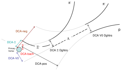
Figure 1: Schematic representation of a $\Xi^{-}$ decay with distance of closest approach (DCA) parameters.

In each Au-Au collision event at RHIC energy ($\sqrt{s_{\rm NN}}=200$ GeV) up to several thousand particles are produced. The finite momentum resolution of the TPC causes the primary tracks to not point back exactly to the primary vertex. As a result, these tracks may randomly cross with other primary tracks and form fake secondary vertices. Indeed, in the quagmire of particle tracks, the vertices can be quite easily misidentified, leading to a large combinatoric background. To reduce this background, basic cuts are applied during the event reconstruction chain.

To determine if two tracks are originated from the same vertex, a cut is placed on their distance of closest approach (DCA). This cut reduces the random background by a large amount, but is insufficient to guarantee a good identification of the parent particle. Other cuts are necessary because of the following reasons:

Table 2: Track quality and kinematic cuts for $\Xi^{-}$ reconstruction.

Track Selection Criteria	loose cut	tight cut
V0 Vertex Cuts:
proton TPC hits	$\geq$15	$\geq$20
pion TPC hits	$\geq$15	$\geq$17
pion and proton PID (for $0.0<p_{\rm t}<2.0$ GeV/$c$)	$\leq 3\sigma$	$\leq 3\sigma$
Track proton DCA to primary vertex(cm)	$\geq$0.5	$\geq$0.5
(for $0.0<p_{\rm t}<2.0$ GeV/$c$)
Track pion DCA to primary vertex (cm)	$\geq$2.0	$\geq$2.0
DCA between V0 daughters (cm)	$\leq$0.7	$\leq$0.65
V0 DCA to primary vertex (cm)	$\geq 0$ and $\leq$0.7	$\geq 0.35$ and $\leq 0.7$
V0 decay length from primary vertex ($r1$)(cm)	$\geq$5.0	$\geq$5.0
$\Xi$ Vertex Cuts:
V0 mass window (Mev/$c^{2}$)	$\pm 7$	$\pm 4$
bachelor $\pi^{-}$ TPC hits	$\geq$10	$\geq$17
bachelor $\pi^{-}$ DCA to primary vertex (cm)	$\geq$0	$\geq$0.5
bachelor PID (for $0.0<p_{\rm t}<2.0$ GeV/$c$)	$\leq 3\sigma$	$\leq 3\sigma$
bachelor $p_{\rm t}$ (GeV/$c$)	$\geq 0.075$	$\geq 0.075$
DCA between $\Xi$ daughters (cm)	$\leq$0.7	$\leq$0.65
angle between $\Xi$’s momentum and decay vertex vector	$\leq\arccos(0.9)$	$\leq\arccos(0.9)$
$\Xi$ DCA to primary vertex (cm)	$\leq$1.0	$\leq$0.5
$\Xi$ decay length from primary vertex ($r2$)(cm)	$\geq 2.0$ and $\leq r1$	$\geq 2.5$ and $\leq r1$

• Due to high density of tracks near the primary vertex, it is easy to form many fake track crossings. This leads to a larger combinatoric background as one gets closer to the primary vertex. The decay distance distribution has an exponential fall-off to zero, so cuts used on these distances for the candidate $\Xi^{-}$ and daughter $\Lambda$ are greater than 2cm and 5cm, respectively. The decay distances are measured from the primary vertex.

• The candidate parents, i.e. candidate $\Xi^{-}$’s, point back to the primary vertex since they are produced at this vertex.

• The daughter tracks do not point back to the primary vertex to ensure they are not primary tracks.

• A cut on the calculated mass of the daughter neutral particle is added to increase the likelihood that the parent particle did indeed decay into a $\Lambda$ ($\bar{\Lambda}$) plus a charged track.

Typical cuts used for $\Xi^{-}$ are listed in Table 2. For track pairs passed all the cuts the invariant mass for a decay vertex is calculated by the kinematic information of its daughters:

$$m=\sqrt{\left(\sqrt{m_{1}^{2}+P_{1}^{2}}+\sqrt{m_{2}^{2}+P_{2}^{2}}\right)^{2}-P^{2}},$$

where subscripts 1 and 2 represent the two daughter particles from a decay vertex. This equation is used twice since there are two decay steps associated with a $\Xi^{-}$ particle. For $\Lambda$ reconstruction one of them is $p$ and the other is $\pi^{-}$. For $\Xi^{-}$ reconstruction one of them is $\Lambda$ and the other is bachelor $\pi^{-}$. $P=P_{1}+P_{2}$ is the parent momentum with $P_{1}$ and $P_{2}$ representing the daughters’ momentum. With all the topological cuts used, clear signal peak is observed in invariant mass distribution.

A tighter cut will make the peak becomes more significant. However, the extremely evil cut results in a high signal-background ratio but at the same time it reduces the signal yield greatly, causing the reconstruction efficiency to be very low.

3 A brief description of neural network and boosting technique

The neural network approach is nothing but functional fitting to data. In classification cases, one wants to construct a mapping $F$ between a set of observable quantities $x_{i}$ ($i=1,\dots,s$) and category variable $Y$ by fitting $F$ to a set of $M$ known “training” samples $(x_{i}^{(p)},y_{k}^{(p)},\,i=1,\dots,s;\,k=1,\dots,v)(p=1,\dots,M,\,y_{k}\in Y)$. Once the parameters in $F$ are fixed, one then uses this parametrization to interpolate and find the category of “test” samples not included in the “training” set. Obviously, the performance of the network on the test set estimates the generalization ability of the fitting. In the present work we use the multilayer perceptron program developed in ROOT version 4.00/04 [15]. The function $F$ is an expansion of sigmoidal function in a feed forward network structure since there is a theorem [14] saying that a linear combination of sigmoids can approximate any continuous function.

A typical three-layer neural network is sketched in figure 3. It consists of an input layer, a hidden layer and an output layer, with various number of nodes (also called neurons) in each layer. In the following, we will use the notation [$s$-$u$-$v$] to denote a neural network with $s$ input nodes, $u$ hideen nodes and $v$ output nodes. There are weights connecting the nodes from any two adjacent layers and each node in the hidden and the output layers has a threshold. The output of the $k$th node in the output layer ($k=1,\dots,v$) is

$$O_{k}(x_{1},x_{2},\cdots,x_{s})=f\left(\sum_{j=1}^{u}w^{\prime}_{jk}x^{\prime}_{j}-\theta^{\prime}_{k}\right)=f\left(\sum_{j=1}^{u}w^{\prime}_{jk}f\left(\sum_{i=1}^{s}w_{ij}x_{i}-\theta_{j}\right)-\theta^{\prime}_{k}\right),$$

where $\{x_{i}\}$ are the input parameters, $\{w_{ij}\}$ are weights between the $i$th node in the input layer and the $j$th node in the hidden layer, $\{\theta_{j}\}$ are thresholds of each node in the hidden layer, $\{w^{\prime}_{jk}\}$ are weights between the $j$th node in the hidden layer and the $k$th node in the output layer, $\{\theta^{\prime}_{k}\}$ are thresholds of each node in the output layer. $f(x)=1/(1+e^{-x})$ is the sigmoid transfer function.

The goal of adjusting the parameters, or training the neural network, is to minimize the fitting error. The mean square error $E$ averaged over the training samples is defined as

$$E={1\over{2M}}\sum_{p=1}^{M}\sum_{k=1}^{v}(O_{k}^{(p)}-y_{k}^{(p)})^{2},$$

where $O_{k}$ is the output of the $k$th node of the neural network, $y_{k}$ is the training target, $M$ is the number of samples in the training set. In binary case, the output layer has only one node, $v=1$, with $y_{1}=0$ for background and $y_{1}=1$ for signal. There are several algorithms for error minimization and weight updating, which are implemented in ROOT as options. The initial weights are random numbers in the range $(-0.5,0.5)$.

Figure 2: A sketch of multilayer perceptron.

Figure 3: The distribution of signal and background from the two-dimensional toy model, where crosses are signals and circles are backgrounds.

Boosting is a technique to construct a committee of weak learners that lowers the error rate in classification. It is first developped by Schapire [16] and the theoretical study followed shows that given a significant number of weak learners, the boosting algorithm can decrease the error rate on the training set and convert the ensemble of weak learners to a strong learner whose error rate on the ensemble is arbitrarily low [17][18]. In the binary classification case, one only needs to construct weak learners with error rate be slightly better than random guessing (0.5). There are a number of variations on basic boosting. The most popular one, AdaBoost, allows the designer to continue adding weak learners until the desired low training error has been achieved. In AdaBoost each training sample receives a distribution $D(p)$ that determines its probability of being selected in a training set for individual component classfier. The distribution $D(p)$ is determined in the following way — if a training sample is accurately classified, then its chance of being used again in a subsequent component classifier is reduced; conversely, if the pattern is not accurately classified, then its chance of being used again is raised. Thus AdaBoost “focuses” the component classifier on more informative or more “difficult” samples.

The AdaBoost procedure for neural network in binary case is as follows:

Input: sequence of $M$ examples $({\bm{x}}^{1},y^{1}),\dots,({\bm{x}}^{M},y^{M})$ with labels $y^{p}\in\{0,1\}$, here ${\bm{x}}={\{x_{i}\}}\,(i=1,\dots,s)$.

Init: $D_{0}(p)=1/M$ for all $p$.

Repeat ($t=0,\dots,T$):

• Train neural network with respect to distribution $D_{t}$ and obtain hypothesis $h_{t}:X\rightarrow Y$,

• calculate the weighted error of $h_{t}:$ $\epsilon_{t}=\sum_{p:h_{t}({\bm{x}}^{p})\neq y^{p}}D_{t}(p)$ and abort loop if $\epsilon_{t}>{1\over 2}$,

• set $\alpha_{t}={1\over 2}\ln{{1-\epsilon_{t}}\over\epsilon_{t}}$,

• update distribution $D_{t}$

  $$D_{t+1}(p)={D_{t}(p)\over Z_{t}}\times\left\{\begin{array}[]{ll}e^{\alpha_{t}}&\mbox{ if }h_{t}({\bm{x}}^{p})\neq y^{p}\mbox{ (incorrectly classified),}\\ e^{-\alpha_{t}}&\mbox{ if }h_{t}({\bm{x}}^{p})=y^{p}\mbox{ (correctly classified),}\end{array}\right.$$

  where $Z_{t}$ is a normalizing constant.

Output: final hypothesis: $h_{\rm final}({\bm{x}}^{p})=\arg\max\limits_{y}\sum\limits_{t}\alpha_{t}h_{t}({\bm{x}}^{p})$.

In binary case the final hypothesis can be restated as

$$h_{\rm final}({\bm{x}}^{p})=\left\{\begin{array}[]{l}1\quad\mbox{ if }\sum_{t=1}^{T}\alpha_{t}h_{t}({\bm{x}}^{p})\geq{1\over 2}\sum_{t=1}^{T}\alpha_{t},\\ 0\quad\mbox{ otherwise.}\end{array}\right.$$

4 A two-dimensional toy model

In high energy physics, the separation of signal from background is a typical binary case. Assume a data set with $n_{s}$ signals and $n_{b}$ backgrounds. Neural network is applied to it and the result can be denoted by the following quantities:

• $n_{cs}:$ the number of signals correctly classified

• $n_{ws}:$ the number of signals incorrectly classified

• $n_{cb}:$ the number of backgrounds correctly classified

• $n_{wb}:$ the number of backgrounds incorrectly classified

The classification ability of the neural network can be judged by the error rate, classification efficiency and signal-background ratio, with the definitions:

$$\mbox{error rate}={{n_{ws}+n_{wb}}\over{n_{s}+n_{b}}},\qquad\mbox{efficiency}={n_{cs}\over n_{s}},\qquad\mbox{S-B ratio}={n_{cs}\over n_{wb}}.$$

According to the above definition, even though boosting is capable in decreasing the error rate of the training set, this does not imply that the classification efficiency and signal-background ratio could be increased. In physics, what is most sought for is high efficiency and high signal-background ratio.

In this section we construct a two-dimensional toy model to show how the boosting algorithm works with neural network for the case of non-overlapping boundary between signal and background, cf. figure 3. In the figure, crosses are signals and circles are backgrounds. The boundary between them is irregular but does not overlap.

To train the neural network we require similar signal- and background- sample-density in the phase space of the training set. Thus 1000 signals and 4000 backgrounds are used to form the training set and another set with the same amount of samples are used as test set. The inputs of the network are the coordinates of the points in X-Y plane. Firstly, we choose a three-layer network [2-10-1] with two input nodes, ten hidden nodes and one output node. All the other network parameters take the default values from ROOT. In Figure 4 are shown the error rate, the classification efficiency and the signal-background ratio of the classification for both training and test sets during being boosted one hundred rounds. We see that with respect to the boosting round, the error rates of the training and test sets decreas sharply while the classification efficiency increases at the first few rounds then slightly oscillates afterwards. The signal-background ratio also increases. Obviously, a boosted neural network can distinguish signal from background better than single neural network with the same network parameters.

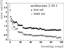
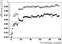
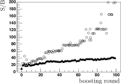
Figure 4: The error rate, classification efficiency and signal-background ratio of the classification by boosted neural network for both training and test sets under the network architecture 2-10-1.

Table 3: The error rate, classification efficiency and signal-background ratio of the classification by single and boosted neural networks with different network architectures and different initial weight matrices in test set for the two-dimensional toy model. w1–w7 indicate seven different initial weight matrices.

• architecture			w1	w2	w3	w4	w5	w6	w7
  		error rate (%)	5.94	4.93	4.46	4.30	5.90	4.40	5.96
  	single	efficiency (%)	89.1	78.6	92.9	93.7	89.6	93.3	89.0
  2-5-1		S-B ratio	4.74	3.42	6.11	6.16	4.69	6.10	4.73
  		error rate (%)	1.04	0.60	0.52	0.94	0.94	0.94	0.98
  	boosted	efficiency (%)	96.9	97.4	99.4	96.5	98.4	97.4	97.2
  		S-B ratio	46.1	34.8	49.7	80.4	31.7	46.4	46.3
  		error rate (%)	2.94	4.10	4.68	3.26	2.66	3.08	3.06
  	single	efficiency (%)	94.6	92.4	89.7	92.6	94.2	93.6	94.5
  2-10-1		S-B ratio	10.2	7.16	6.85	10.4	12.6	10.4	9.64
  		error rate (%)	0.88	1.10	0.94	1.04	1.02	0.98	0.88
  	boosted	efficiency (%)	97.3	96.7	97.0	97.4	98.2	97.5	97.5
  		S-B ratio	57.3	44.0	57.1	37.5	29.8	40.6	51.3
  		error rate (%)	2.32	1.48	1.6	2.38	1.46	1.54	2.38
  	single	efficiency (%)	93.0	95.6	95.6	92.4	95.8	95.6	94.4
  2-5-4-1		S-B ratio	20.2	31.9	26.6	21.5	30.9	28.9	15.0
  		error rate (%)	0.88	0.64	0.94	0.60	0.88	0.76	0.70
  	boosted	efficiency (%)	97.3	98.6	97.0	98.6	97.5	97.6	98.8
  		S-B ratio	57.2	54.7	57.1	61.6	51.3	75.1	43.0

One of the disadvantages of neural network is that its performance depends on network architecture and initial weight matrices. To study the dependency, we vary the hidden nodes of the network and use different weight matrices. The behavior of the networks in terms of error rate, classification efficiency and signal-background ratio are listed in Table 3.

It can be seen from the table that, in average, more complicated single network architecture, e.g. [2-5-4-1], gives out lower error rate, higher efficiency and higher signal-background ratio than the other two architectures, and that for different initial weight matrices the performance of the network varies even for the same architecture. After boosting, not only the error rate decreases but also the classification efficiency and signal-background ratio increase in comparison to those of the single neural network. In addition, the dependency of the network performance on different network architectures and initial weight matrices vanishes. Therefore, boosted simple neural network with arbitrary initial weight matrices has comparable ability as a single neural network with a complicated structure and fine-tuned parameters.

5 Classification of quark- and gluon- jets

The Monte Carlo JetSet7.4 is used to generate $\rm e^{+}\rm e^{-}$ collision events at 91.2 GeV. The quark- and gluon- jet samples are obtained through the following procedure: (1) Force events into 3-jet ones both at parton and at hadron levels by using the Durham jet algorithm [19]. (2) Select the planar 3-jet events by requiring the sum of the three angles between two adjacent jets to be greater than $358^{\circ}$ at hadron level (this condition is automatically satisfied at parton level). (3) Apply the angular cut method [20] to the hadronic 3-jet event, i.e. the three angles between two adjacent jets are ordered and the jet opposite to the largest angle is supposed to be a gluon jet and the jet opposite to the smallest angle is the more energetic quark jet. We require the difference between the largest angle and the middle one to be greater than an angular cut $20^{\circ}$ and the more energetic quark jet is rejected in an event. (4) Match the hadronic quark- and gluon- jets with the corresponding parton level jets. Four variables are chosen to describe a jet, i.e. the multiplicity $n$ inside jet, the transverse momentum $p_{\rm t}$ of jet, the included angle $\theta$ opposite to the jet and the jet energy $E_{\rm vis}$.

Usually, the quark and gluon jet samples are hard to be distinguished because of the large overlapping of these two sets. Using the above procedure, the quark- and gluon- jet samples are well selected from the generated raw samples and the overlapping in some phase space is decreased, so that we can study how the network works and compare it with the simple cut method.

In Figure 6 is shown the mixing region of quark- and gluon- jets in $E_{\rm vis}$ and $\theta$ space. Compared with the simple two-dimensional toy model, the boundary is unclear and the two sets overlap each other strongly. If we apply a $\theta$ cut, e.g. setting $\theta\geq 2.675$ to be gluon jet and $\theta<2.675$ to be quark jet, the efficiency for both quark- and gluon- jets are greater than $90\%$ and the error rate is $4.05\%$

Figure 5: The distribution of quark- and gluon- jets near their boundary. Crosses represent quark jets and circles represent gluon jets.

Figure 6: The error rate of the classification of quark and gluon jet samples by boosted neural network both for training set and for test set under network architecture 4-5-1.

Next, we take 2500 quark jets and 2500 gluon jets as training set and another 5000 as test set. From the above two-dimensional toy model we know that boosting different network architectures will result in similar performance, so we choose a very simple network architecture [4-5-1] to save the computer time and ensure network generalization ability.

In figure 6 are plotted the error rates of the network in the training and test sets versus the boosting round. It can be seen from the figure that the error rates increase in the first boosting round then decrease afterwards. For the training set the error rate decreases to zero while for the test set, the error rate decreases slightly and oscillates, keeping higher than that of the first round. To check the results we tried a more complicated network architecture [4-50-1] to do the boosting. The similar trends are obtained. The comparison of single neural network, boosted network and simple cut method with respect to error rate, efficiency and signal-background ratio are shown in Table 5. It can be seen that, although the boosted neural network does not work well for the present case, the single neural network still presents lower error rate, higher efficiency and higher signal-background ratio in comparison with the simple cut method.

Table 4: The error rate, classification efficiency and signal-background ratio of the single neural network, the first boosting round and the boosted neural network with different network architectures and different initial weight matrices for test set in the case of quark- and gluon-jets classification.

		error rate (%)			efficiency(%)			S-B ratio
Methods
		w1	w2	w3	w1	w2	w3	w1	w2	w3
	single	1.42	1.38	1.50	98.80	98.80	98.64	60.2	63.3	60.2
4-5-1	1st round	2.22	2.46	2.12	97.96	98.32	98.00	40.8	30.3	43.8
	boosted	1.82	1.60	1.50	98.08	98.32	98.28	57.0	64.7	76.8
	single	1.36	1.34	1.38	98.80	98.80	98.72	65.0	66.8	66.7
4-50-1	1st round	2.72	2.70	2.58	97.68	97.36	97.84	31.3	35.3	32.6
	boosted	1.68	1.72	1.66	98.28	98.04	98.28	59.9	66.2	61.4
simple	cut		4.05			97.65			18.0

6 Discussions

In this paper we apply the boosting technique to artificial neural network. A two-dimensional toy model is constructed to show how boosted neural network works when the boundary between signal and background is complicated but does not overlap. Then the boosted neural network is applied to Monte Carlo quark- and gluon- jet samples of e⁺e^-collision, where the two samples strongly mix with each other.

In both cases the boosting technique drives the error rate of the training set to zero, while the error rates of the test sets behave differently. In the case of two-dimensional toy model with non-overlapping boundary, the error rate of the test set also decreases dramatically but in the case of quark- and gluon- jet samples with strong overlap, the error rate of the test set increases at the first boosting round then decreases slightly. We also tried some other event samples, for example, a tighter or looser angular cut mentioned in section 5 or cuts on the network input parameter, the included angle $\theta$, are applied to quark and gluon jets to make the classification task easier or harder. We found that once there are mixing between quark-jet set and gluon-jet set, the performance of boosted neural networks is similar as that shown above. So we conclude that boosting technique does not improve the performance of single neural networks in the case of overlapping samples like the quark and gluon jets. This is easy to understand since boosting technique is always applied to unstable classifiers, while we see that from table 5 the outcomes of single neural network are rather stable at different network architectures and initial weight matrices. There is no space for boosting technique to improve the behavior of single neural networks in this case.

To summarize, artificial neural network, in general, results in lower error rate than simple cut method. Boosted neural network avoids the disadvantage of single neural network and is more stable and easier to implement. It will lower the error rate, increase the efficiency and signal-background ratio of classification in case the boundaries between signal and background are complicated but separable which could not be easily classified by simple cut method. While for the case with mixed signal and background, the boosted neural network does not help improving the classification.

References

References

- [1] Lansdell C. P. L. 2002 Charged Xi Production in 130 GeV Au-Au Collision at the Relativistic Heavy Ion Collider, PhD thesis (The University of Texas at Austin) p77.
- [2] Denby B 1988 Comput. Phys. Commun. 49 429.
- [3] Lönnblad L, Peterson C and Rögnvaldsson T 1990 Phys. Rev. Lett. 65 1321.
- [4] Csabai I, Czak F and Fodor Z 1991 Phys. Rev. D 44 1905.
- [5] Chattopadhyaya S, Ahammed Z and Viyogi Y P 1999 Nucl. Instrum. Meth. A 421 558.
- [6] D0 Collaboration, Abazov V M et al. 2001 Phys. Lett. B 517 282.
- [7] Boos E and Dudko L 2003 Nucl. Instrum. Meth. A 502 486.
- [8] Maggipinto T, Nardulli G, Dusini S, Ferrari F, Lazzizzera I., Sidoti A, Sartori A and Tecchiolli G P 1997 Phys. Lett. B 409, 517.
- [9] Roe B P, Yang H J, Zhu J, Liu Y, Stancu I and McGregor G 2005 Nucl. Instrum. Meth. A 543 577.
- [10] Drucker H, Schapire R and Simard P 1993 International Journal of Pattern Recognition and Artificial Intelligence, 7(4) 705.
- [11] Drucker H 1999 Combining Artificial Neural Nets: Ensemble and Modular Learning(NewYork: Springer-Verlag) p 51-77.
- [12] Schwenk H and Bengio Y 1997 International Conference on Artificial Neural Networks(ICANN’97) (Springer) p 967-972.
- [13] Particle Data Group 2002 Review of Particle Physics, Phys. Rev. D66 010001.
- [14] K.Hornik et al. 1989 Neural Networks 2 359.
- [15] http://root.cern.ch/root/html//TMultiLayerPerceptron.html
- [16] Schapire R E 1990 Machine Learning 5(2) 197.
- [17] Freund Y and Schapire R E 1997 Journal of Computer and System Sciences 55(1) 119.
- [18] Friedman J, Hastie T and Tibshirani R 2000 The Annals of Statistics 28(2) 337.
- [19] Dokshitzer Yu J 1991 J. Phys. G 17 1537.
- [20] Yu M L and Liu L S 2002 Chinese. Phys. Lett. 19, 647.