Nonlinear Inflaton Fragmentation after Preheating

Abstract

We consider the nonlinear dynamics of inflaton fragmentation during and after preheating in the simplest model of chaotic inflation. While the earlier regime of parametric resonant particle production and the later turbulent regime of interacting fields evolving towards equilibrium are well identified and understood, the short intermediate stage of violent nonlinear dynamics remains less explored. Lattice simulations of fully nonlinear preheating dynamics show specific features of this intermediate stage: occupation numbers of the scalar particles are peaked, scalar fields become significantly non-gaussian and the field dynamics become chaotic and irreversible. Visualization of the field dynamics in configuration space reveals that nonlinear interactions generate non-gaussian inflaton inhomogeneities with very fast growing amplitudes. The peaks of the inflaton inhomogeneities coincide with the peaks of the scalar field(s) produced by parametric resonance. When the inflaton peaks reach their maxima, they stop growing and begin to expand. The subsequent dynamics is determined by expansion and superposition of the scalar waves originating from the peaks. Multiple wave superposition results in phase mixing and turbulent wave dynamics. Thus, the short intermediate stage is defined by the formation, expansion and collision of bubble-like field inhomogeneities associated with the peaks of the original gaussian field. This process is qualitatively similar to the bubble-like inflaton fragmentation that occurs during tachyonic preheating after hybrid or new inflation.

I Introduction

The origin of matter in the universe from a decaying inflaton field in the process of (p)reheating is a basic feature of all realistic inflationary models. If four dimensional effective field theory is sufficient (for specifics of reheating in string theory inflation see e.g. KY ) this process is described by the non-equilibrium QFT of particle creation and thermalization. In chaotic inflation this particle creation typically involves a period of parametric resonance, when occupation numbers of Bose particles rapidly become exponentially large KLS . In this case the QFT is well approximated by classical field theory, which can be investigated in detail with classical lattice simulations lattice . A full treatment of the quantum field theory of the non-linear stages of preheating in controllable models in the limit of high occupation numbers is in agreement with the classical approximation berges .

The simplest possible inflationary potential contains a massive inflation field $V=\frac{1}{2}m^{2}\phi^{2}$ and the simplest preheating model involves a coupling of the inflaton to another field $\frac{1}{2}g^{2}\phi^{2}\chi^{2}$. The regime of parametric resonant particle production is understood analytically KLS . Backreaction of inhomogeneous fluctuations quickly brings the system of interacting scalar fields to a strongly non-linear regime characterized by very high occupation numbers. The turbulent regime of interacting classical scalar field waves was studied in detail in numerical simulations lattice ; MT ; FK , most of which are based on the LATTICEASY code FT , and in the $\lambda\phi^{4}$ model even analytically with the kinetic theory of Kolmogorov-type turbulence MT . The least understood stage of (p)reheating is the short, violent transition from linear preheating to the turbulent stage, which shows anomalies in the momentum space picture, and in the departure from gaussian statistics FK .

Hybrid inflation is another very important class of inflationary models. At first glance preheating in hybrid inflation, which contains a symmetry breaking mechanism in the Higgs field sector, has a very different character than in chaotic inflation. Preheating in hybrid inflation occurs via tachyonic preheating GBFKLT , in which a tachyonic instability of the homogeneous modes drives the production of field fluctuations. In hybrid inflation, the decay of the homogeneous fields leads to fast non-linear growth of scalar field lumps associated with the peaks of the initial (quantum) fluctuations. The lumps then build up, expand and superpose in a random manner to form turbulent, interacting scalar waves GBFKLT ; lumps . A similar picture emeres in new inflation preheating new . Like parametric resonance, tachyonic preheating can be interpreted via the reciprocal picture of copious particle production far away from thermal equilibrium, and consequent cascades of energy through interacting, excited modes.

In this paper we investigate in detail the structure of preheating after chaotic inflation in configuration space. We find that the intermediate stage between linear preheating and turbulence proceeds via non-linear growth, expansion, and superposition of large value field bubbles, similar to what we earlier observed in hybrid inflation. Thus, the bubble-like intermediate structure of the non-linear fields is another consistent feature of preheating. However, the details of the non-linear dynamics are different: while the bubbles in preheating after hybrid inflation initially occur as isolated patches with large spaces in between them, the bubbles that appear in preheating in the model being considered here appear more densely throughout the space and persist for some time as a pattern of standing waves before they begin spreading and colliding.

In section II we describe the model we are considering and review the basic nature of preheating in this model, focusing on the (well studied) behavior of the fields in momentum space. In section III we discuss different diagnostics of the system of interacting scalar fields in configuration space and describe the fully non-linear dynamics of inflaton fragmentation. In the concluding section we discuss some of the implications of these results, in particular, for the generation of gravitational waves from preheating and baryo/leptogenesis from preheating.

II Preheating and Thermalization in Momentum Space

We consider the potential

$$V={1\over 2}m^{2}\phi^{2}+{1\over 2}g^{2}\phi^{2}\chi^{2}$$ (1)

where $\phi$ is the inflaton and $\chi$ is another scalar field that is coupled to it. At the end of inflation $\phi$ is a homogeneous field which oscillates as $\phi(t)\approx\frac{M_{p}}{\sqrt{3\pi}mt}\,\sin mt$ and $\chi$ is a quantum field with eigenfunctions $\chi_{k}(t)e^{-i{\bf kx}}$. The temporal part $\chi_{k}(t)$ obeys an oscillator equation with a periodic frequency $\omega_{k}^{2}=(k^{2}/a^{2})+g^{2}\phi(t)^{2}$. The amplitude $\chi_{k}(t)$ thus undergoes parametric resonance, leading to large occupation numbers of created particles $n_{k}$.

Due to the rapid growth of its occupation numbers the field $\chi(t,\vec{x})$ can be treated as a classical scalar field. Its appearance is described by the realization of the random gaussian field

$$\chi(t\ ,\vec{x})=2\,\int d^{3}k\,|\chi_{k}(t)|\,\cos({\bf kx}+\theta_{k})$$ (2)

i.e. as a superposition of standing waves with random phases $\theta_{k}$ and Rayleigh-distributed amplitudes $P(|\chi_{k}(t)|)d|\chi_{k}(t)|=e^{-\frac{|\chi_{k}(t)|^{2}}{\Delta}}\,\frac{2|\chi_{k}(t)|}{\Delta}\,d|\chi_{k}(t)|$, $\Delta=<|\chi_{k}(t)|^{2}>$. One can use many different quantities to characterize a random field, such as its variances $<\sigma^{2}_{n}>=\int d^{3}k\,k^{2n}\,|\chi_{k}(t)|^{2}$, the spatial density of its peaks of a given height, etc. The scale of the peaks and their density depend on the characteristic scale $R$ of the spectrum, which in our case is related to the leading resonant momentum $k_{*}\simeq\sqrt{gm\phi_{0}}a^{1/4}$ KLS . At the linear stage the phases $\theta_{k}$ are constant, so that the structure of the random field $\chi$ stays almost the same.

Once one field is amplified in this way, other fields that are coupled to it are themselves amplified FK , so within a short time of linear preheating (of order dozens of inflaton oscillations) fluctuations of $\chi$ generate inhomogenoeus fluctuations of the field $\phi$. It is easy to see that fluctuations of $\phi$ will have a non-linear, non-gaussian character. From the equation of motion for $\phi$

$$\Box\phi+m^{2}\phi^{2}+g^{2}\chi^{2}\phi=0\ ,$$ (3)

we have in Fourier-space

$$\ddot{\phi}_{k}+3H\dot{\phi}_{k}+\left((k^{2}/a^{2})+m^{2}\right)\phi_{k}=g^{2}\phi_{0}(t)\,\int d^{3}q\,\chi_{q}\chi^{*}_{k-q}\ ,$$ (4)

where we neglect the term that is third order with respect to fluctuations; $\phi_{0}(t)$ is the background oscillation. The solution of this equation with Green’s functions KLS shows that $\phi$ fluctuations grow with twice the exponent of $\chi$ fluctuations. It also shows that the fluctuations of $\phi$ are non-gaussian. Sometimes this solution is interpreted as re-scattering of the particle $\chi_{q}$ against the condensate particle $\phi_{0}$ at rest producing $\chi_{k-q}$ and $\phi_{k}$, $\chi\phi_{0}\to\chi\delta\phi$. As we will see shortly, this interpretation has significant limitations.

When the amplitudes of $\chi$ and $\phi$ become sufficiently large we have to deal with the fully non-linear problem. The field evolution can be well approximated using the classical equation of motion (3) supplemented by another equation for $\chi$

$$\Box\chi+g^{2}\phi^{2}\chi=0\ .$$ (5)

Results of simulations of non-linear preheating using the LATTICEEASY program FT have been reported in many earlier papers lattice ; FK . For chaotic inflation, these results were presented in terms of the time evolution of occupation numbers $n_{k}(t)$ or total number density of particles $N(t)$. Figures 1-3 show the results of our simulations in these familiar terms of $n_{k}(t)$ (in combination $k^{3}\omega_{k}n_{k}$) and $N(t)$, as well as showing the evolution of the field statistics (departures from gaussianity). Here and for the rest of this paper all simulation results are for model (1) with $m=10^{-6}M_{p}$ (fixed by CMB normalization) and $g^{2}=2.5\times 10^{-7}$. The size of the box was $L=10m^{-1}$ and the grid contained $256^{3}$ points. We also tried other values of $g^{2}$ and found qualitatively similar results.

Figure 1 shows the evolution of the spectra. The spectra show rapid growth of the occupation numbers of both fields, with a resonant peak that develops first in the infrared ($k\simeq k_{*}$) and then moves towards the ultraviolet as a result of rescattering. In figure 3 you can see clearly that the occupation number of $\chi$ initially grows exponentially fast due to parametric resonance, followed by even faster growth of the $\phi$ field due to the interaction, in accordance with the solution of eq (4).

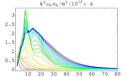
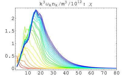
Figure 1: Evolution of spectra in the combination $k^{3}\omega_{k}n_{k}$ of the $\phi$ and $\chi$ fields during and immediately after preheating. Bluer plots show later spectra. Horizontal axis $k$ is in units of $m$

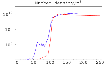
Figure 2: Evolution of comoving number density of $\phi$ (red, lower plot) and $\chi$ (blue, upper plot) in units of $m^{3}$. Time is in units of $1/m$

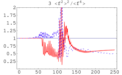
Figure 3: Evolution of the ratio $\langle f^{2}\rangle^{2}/\langle f^{4}\rangle$, where $f$ represents the $\phi$ field (red, solid) or the $\chi$ field (blue, dashed) and angle brackets represent a spatial average, is a measure of gaussianity. This ratio is one for a random gaussian field. Time is in units $1/m$

The gaussianity of classical fileds can be measured in different ways. In Figure 3 we show the evolution of the ratio $\langle f^{2}\rangle^{2}/\langle f^{4}\rangle$ (kurtosis), which is equal to unity for a gaussian field. During the linear stage of preheating, the field fluctuations are a random gaussian field, see eq. (2), reflecting the initial quantum fluctuations that seeded them. The inhomogenoeus field $\phi$ is generated as a non-gaussian field, in agreement with the solution of eq (4). When the fluctuation amplitude begins to get large, both fields are non-gaussian. During the later turbulent stage both fields begin to return to gaussianity.

Another known feature of preheating is the onset of chaos, when small differences in the initial conditions for the fields lead to exponentially divergent solutions: $D(t)\simeq e^{\lambda t}$, where $D$ is the distance in phase space between the solutions and $\lambda$ is the Lyapunov exponent (see FK for details). The distance $D$ begins to diverge exponentially exactly after the violent transition to the turbulent stage.

Let us summarize the picture which emerges when we study preheating, turbulence and thermalization in momentum space with the occupation numbers $n_{k}$. There is initial exponential amplification of the field $\chi$, peaked around the mode $k_{*}$. At this stage the $\chi$ fluctuations form a squeezed state, which is a superposition of standing waves that make up a realization of a random gaussian field. Interactions of the two fields lead to very rapid excitation of fluctuations of $\phi$, with its energy spectrum also sharply peaked around $k_{*}$. To describe generation of $\phi$ inhomogeneities, people use the terminology of “re-scattering”of waves. However, there is a short violent stage when occupation numbers have a sharply peaked and rapidly changing spectrum. The field at this stage is non-gaussian, which signals that the waves phases are correlated. In some sense, the concept of “particles” is not very useful around that time. In the later turbulent stage when $n_{k}(t)$ gradually evolves and gaussianity is restored (due to the loss of phase coherency) the picture of rescattering particles becomes proper. As we will see in the next section, gaussianity is not restored for some time after the end of preheating. To understand this violent, intermediate stage, however, it is useful to turn to the reciprocal picture of field dynamics in configuration space.

III Inflaton Fragmentation in Configuration Space

The features in the occupation number spectra $n_{k}(t)$, namely, sharp time variations, peaks at $k\sim k_{*}$, and strong non-gaussianity of the fields around the time of transition between preheating and turbulence suggest that we dealing with distinct spatial features of the fields in the configuration space. This prompted us to study the dynamics of the fields in configuration space.

The evolution of the fields in configuration space is shown in Figure 4. Each frame shows the spatial profile of the fields $\phi$ and $\chi$ along a two-dimensional slice of the 3D lattice. A movie that includes many more time frames can be found at http://www.science.smith.edu/departments/Physics/fstaff/gfelder/public/bubbles/. Note that here (and everywhere in this paper) times are reported in units of $1/m$.

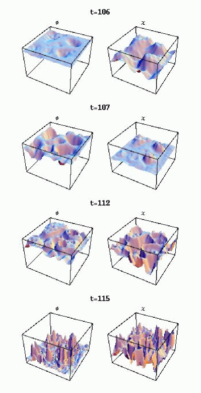
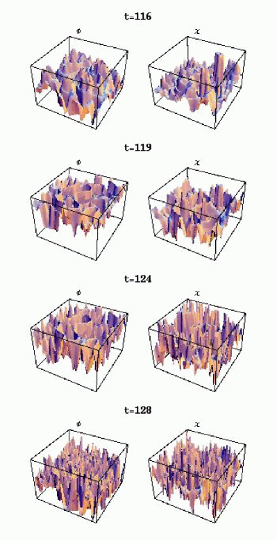
Figure 4: Values of the $\phi$ and $\chi$ fields in a two dimensional slice through the lattice. The horizontal axes are spatial axes and the vertical axis is field value.

The initial evolution of the fields ($t\mathrel{\hbox{\hbox to0.0pt{\hbox{\lower 4.0pt\hbox{$\sim$}}\hss}\hbox{$<$}}}100$) is characterized by linear growth of fluctuations of $\chi$. During this stage the fluctuations have the form of a superposition of standing waves with random phases, which make up a random gaussian field (2). The eye captures positive and negative peaks that correspond to the peaks of the initial gaussian random field $\chi$. The peaks in this early stage correspond to the peaks of the initial gaussian random field $\chi$. Next the oscillations of $\chi$ excite oscillations of $\phi$. The first panel of Figure (4) shows a typical profile near the end of this period, just as the oscillations are becoming nonlinear and $\phi$ is becoming excited. The amplitude of these $\phi$ oscillations grows much faster than the initial $\chi$ oscillations (see our discussion of eq. (4)) and the oscillations have different (and changing) frequencies. The peaks of the $\phi$ oscillations occur in the same places as the peaks of the $\chi$ oscillations, however, as can be seen in the bottom three panels on the left side of Figure (4). We can analyze the evolution during this early non-linear period, not using the Fourier-mode description (4), but instead considering the configuration space description equation (3). The interaction term in the equation of motion is approximated during this stage by $g^{2}\phi_{0}\chi^{2}$, so we have

$$\phi(t,{\bf x})=\phi_{0}(t)+g^{2}\int d^{4}x^{\prime}\,\phi_{0}(t^{\prime})\,\chi^{2}(t^{\prime},{\bf x^{\prime}})G(s)\ ,$$ (6)

where $G(s)$ is the retarded Green’s function of the massive scalar field wave equation, $s=(t-t^{\prime})^{2}-({\bf x-\bf x^{\prime}})^{2}$. Thus the profile of $\phi(t,{\bf x})$ is a superposition of the still oscillating homogeneous part plus inhomogeneities induced by the Yukawa-type interaction $(g^{2}\phi_{0})\phi\chi^{2}$ in the Lagrangian. Since the Yukawa interaction is a short-range interaction (defined by the length scale $1/m$ for a space-like interval $G(r)\sim e^{-mr}$), induced inhomogeneities of $\phi$ appear in the vicinity of those in $\chi$.

In the next stage ($t\mathrel{\hbox{\hbox to0.0pt{\hbox{\lower 4.0pt\hbox{$\sim$}}\hss}\hbox{$>$}}}110$) the peaks reach their maximum amplitude, comparable to the initial value of the homogeneous field $\phi$, and begin to spread. The two lower left panels of Figure (4) shows the peaks expanding and colliding. In the panels on the right you can see the standing wave pattern lose coherence as the peaks send out ripples that collide and interfere. By $t=124$ the fluctuations have spread throughout the lattice, but you can still see waves spreading from the original locations of the peaks. Shortly after that time all coherence is lost and the field configurations appear to be like random turbulence.

Figure (5) shows the distribution of energy density at several points during the evolution. Several points about these figures are worth noting. For the parameters we are considering, the gradient energy is subdominant throughout the violent rescattering stage and only begins to be significant during the onset of turbulence. Fluctuations in the potential and kinetic energy grow in the locations of the bubbles seen in figure (4), but they are out of phase such that the total energy density remains nearly homogeneous. Later, as the bubbles spread and collide, the phase coherence is lost and inhomogeneities appear in the total energy density. A movie showing many more time frames of energy density can be found at http://www.science.smith.edu/departments/Physics/fstaff/gfelder/public/bubbles/.

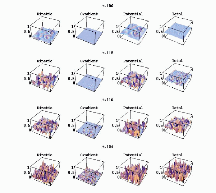
Figure 5: Energy density and its components. The horizontal axes represent the same two dimensional slice through the lattice as in figure (4).

For the first time we calculate the evolution of the statistics of the fields. Figure (6) shows the field distributions (histograms) at various times during the evolution. Initially both fields have gaussian distributions (from their random quantum fluctuations), with $\phi$ sharply peaked around $\phi_{0}$ and $\chi$ centered around zero. As non-linear effects become important, the statistics of both fields become quite non-trivial. The distribution of the inflaton field becomes at times sharply peaked to one side, when the condensate is at an extreme end of its oscillation, and at other times bi-modal, with a distinct presence of the homogeneous component plus a significant inhomogeneous component. The statistics of the $\chi$ field also become strongly non-gaussian. Perhaps most surprisingly, the statistics of both fields remain non-gaussian for a long time after preheating. At the end of our simulation, at $t=300$, the fields were still noticeably non-gaussian. During all this time the random phase approximation of interacting scalars is justified only to the extent that the distributions approximate gaussians.

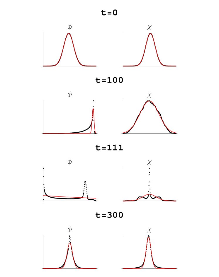
Figure 6: Field distributions. The horizontal axes are field values and the vertical axis represents the frequency of that field value on the lattice. The black dots represent the simulation results and the red lines are best-fit Gaussian curves. The fitting lines can not be seen in the first frame because they lie directly under the dots.

IV Discussion

It is convenient to split the process of transition from the homogeneous inflaton condensate to the radiation of randomly moving waves into four stages: The first is exponentially rapid growth of small inhomogeneities that emerge from vacuum fluctuations. During this stage fluctuations are linear and the fields are gaussian random fields. The second stage is violent backreaction and rescattering of waves, with non-gaussian, nonlinear, nonthermal fluctuations. The third stage is Kolmogorov turbulence. During this period the fluctuations are again (nearly) gaussian and energy gradually cascades towards high momentum modes. Finally, there is thermalization.

In this paper we used lattice simulations to investigate the second stage of violent field restructuring. We considered the model (1), in which preheating occurs through parametric resonance, and examined the evolution of the fields in configuration space. The picture that emerged is similar in many ways to what we observed earlier for tachyonic preheating in hybrid inflation. For instance in the F-term inflation example where the non-linear potential around the bifurcation point is $V(\sigma)=-\frac{\lambda}{3}v\phi^{3}+\frac{\lambda}{4}\phi^{4}+\frac{\lambda}{12}v^{4}$, small initial random fluctuations of $\phi$ are amplified by the non-linear $\phi^{3}$ term. The peaks of the gaussian field thus begin to grow very fast relatively to the surrounding regions of $\phi$. Along those same lines, we found here that oscillations of the $\chi$ and $\phi$ fields grow initially at the locations of the peaks in the initial $\chi$ field. For the model (1) these growing peaks form a pattern of standing waves that persists throughout the linear regime and then begin to spread and overlap as rescattering becomes important.

The bubble-like structure we see here (and in hybrid inflation) has nothing to do with first-order phase transitions, but just with the initial structure of vacuum fluctuations plus non-linear dynamics . Growth of the individual peaks results in the build-up of the scalar field gradients. Subsequent evolution is defined by the expansion of the bubbles. The superposition of many almost spherically expanding bubbles leads to decoherence and turbulent motion of the scalar waves.

The main lesson we have learned from this work is that the preheating stage of linear fluctuations and the turbulent stage of interacting waves are divided by a short, violent stage of non-linear formation and collision of bubble-like large value field regions.

Eventually the fields reach thermal equilibrium characterized only by the temperature. Does that mean that all traces of inflaton fragmentation history are erased? There are potential tracers of the non-linear stage of preheating related to out-of-equilibrium processes. For instance, people have discussed realizations of baryogenesis at the electroweak scale via tachyonic preheating after hybrid inflation GGKS , and this process is ultimately related to the bubble-like lumps of the Higgs field that form during tachyonic preheating GGG . Since we now see that fragmentation through bubbles can also occur in chaotic inflation, baryogenesis via out-of-equilibrium bubbles can also be extended to these models.

There is another, potentially observable consequence of the non-linear “bubble” stage of inflaton fragmentation. Lumps of the scalar fields correspond to large (order of unity) energy density inhomogeneities at the scale of those bubbles, $R$. Collisions of bubbles generate gravitational waves. The fraction of the total energy at the time of preheating converted into gravitational waves is significant. We estimate it is of the order of

$$\frac{\rho_{gw}}{\rho_{rad}}\simeq(RH)^{2}\ ,$$ (7)

where $1/H$ is the Hubble radius. This corresponds to a present-day fraction of energy density $\Omega_{GW}\sim 10^{-5}(RH)^{2}$. The way to understand formula (7) is the following: The energy converted into gravitational waves from the collision of two black holes is of the order of the black hole masses. If the mass of lumps of size $R$ is a fraction $f$ of a black hole of the same size, then the fraction of energy converted to gravitational waves from two lumps colliding is $f$. Scalar field lumps at the Hubble scale would form black holes, so in our case $f=(RH)^{2}$.

The present-day frequency of this gravitational radiation is

$$f\simeq\frac{10^{7}Gev}{M}Hz\ ,$$ (8)

where $M=V^{1/4}$ is the energy scale of inflation with the potential $V$.

For the chaotic inflation model considered in this paper the size of the bubbles is $R\sim few/m$ and at the time they begin colliding $H\sim m/100$, so that the fraction of energy converted into gravitational waves is of the order $10^{-3}-10^{-4}$. This figure is in agreement with the numerical calculations of gravitational wave radiation from preheating after chaotic inflation GW .

For chaotic inflation with $M$ at the GUT scale the frequency (8) is too short and not observable. Gravitational waves continue to be generated during the turbulent stage and even during equilibrium due to thermal fluctuations, but with a smaller amplitude. It is a subject of further investigation if they can be observed. The most promising possibility for observations is, however, generation of gravity waves from low energy hybrid inflation, where $f$ can much much smaller.

We would like to thank Marco Peloso for useful discussions. G.F. was supported by NSF grant PHY-0456631. L.K. wa supported by NSERC and CIAR. G.F. would like to thank the Canadian Institute for Theoretical Astrophysics for their hospitality during part of this work

References

- (1) For specifics of of reheating in string theory inflation see e.g. L. Kofman and P. Yi, Phys. Rev. D 72, 106001 (2005) [arXiv:hep-th/0507257].
- (2) L. A. Kofman, A. D. Linde and A. A. Starobinsky, Phys. Rev. Lett. 73, 3195 (1994); Phys. Rev. D 56, 3258 (1997).
- (3) S. Y. Khlebnikov and I. I. Tkachev, Phys. Rev. Lett. 77, 219 (1996) [arXiv:hep-ph/9603378] ; S. Y. Khlebnikov and I. I. Tkachev, Phys. Rev. Lett. 79, 1607 (1997) [arXiv:hep-ph/9610477] ; T. Prokopec and T. G. Roos, Phys. Rev. D 55, 3768 (1997) [arXiv:hep-ph/9610400].
- (4) J. Berges and J. Serreau, Phys. Rev. Lett. 91, 111601 (2003) [arXiv:hep-ph/0208070] ; J. Berges and J. Serreau, arXiv:hep-ph/0302210 ; J. Berges and J. Serreau, arXiv:hep-ph/0410330 ; J. Berges, S. Borsanyi and C. Wetterich, Phys. Rev. Lett. 93, 142002 (2004) [arXiv:hep-ph/0403234].
- (5) G. Felder and L. Kofman, “The development of equilibrium after preheating,” hep-ph/0011160
- (6) R. Micha and I. I. Tkachev, Phys. Rev. D 70, 043538 (2004) [hep-ph/0403101].
- (7) G. Felder and I. Tkachev, “LATTICEEASY: A program for lattice simulations of scalar fields in an expanding universe,” hep-ph/0011159.
- (8) G. N. Felder, J. Garcia-Bellido, P. B. Greene, L. Kofman, A. D. Linde and I. Tkachev, Phys. Rev. Lett. 87, 011601 (2001) [hep-ph/0012142] ; .
- (9) G. N. Felder, L. Kofman and A. D. Linde, Phys. Rev. D 64, 123517 (2001) [arXiv:hep-th/0106179]; J. Garcia-Bellido, M. Garcia Perez and A. Gonzalez-Arroyo, Phys. Rev. D 67, 103501 (2003) [arXiv:hep-ph/0208228].
- (10) M. Desroche, G. N. Felder, J. M. Kratochvil and A. Linde, Phys. Rev. D 71, 103516 (2005) [arXiv:hep-th/0501080].
- (11) J. Garcia-Bellido, D.Yu. Grigoriev, A. Kusenko, M. Shaposhnikov, “ Nonequilibrium electroweak baryogenesis from preheating after inflation”. Phys.Rev.D60:123504,1999
- (12) J. Garcia-Bellido, M. Garcia-Perez, A. Gonzalez-Arroyo “Chern-Simons production during preheating in hybrid inflation models”. Phys.Rev.D69:023504,2004
- (13) S. Y. Khlebnikov and I. I. Tkachev, Phys. Rev. D 56, 653 (1997) [arXiv:hep-ph/9701423]; R. Easther and E. A. Lim, JCAP 0604, 010 (2006) [arXiv:astro-ph/0601617].