Influence of finite quark chemical potentials on the three flavor LOFF phase of QCD

Abstract

We study in the Ginzburg-Landau approximation, the Larkin-Ovchinnikov-Fulde-Ferrell (LOFF) phase of QCD with three flavors and one plane wave, including terms of order ${\cal O}(1/\mu)$. We show that the LOFF window is slightly enlarged, and actually splits into two different regions, one characterized by $u-s$ and $d-u$ pairings and the other with $d-u$ pairs only.

I Introduction

At high densities and small temperatures quarks are expected to attract each other in the color antisymmetric channel. Cooper pairs are expected to be formed and color superconductivity to arise, see barrois ; Alford:1997zt and Rajagopal:2000wf for reviews of the subject. For three quark flavors, the Color-Flavor-Locking (CFL) phase is known to be the ground state, provided the density is asymptotically high. The condensate is a spinless color- and flavor- antisymmetric diquark Alford:1998mk .

Pre-asymptotic densities and $T\simeq 0$ are probably relevant to describe the cores of compact stars (we will consider only the zero temperature case in this paper). At those densities one cannot neglect the mass of the strange quark and the chemical potential differences $\delta\mu$ due to $\beta$ equilibrium. Much effort has been devoted to study phases which might be relevant at such pre-asymptotic densities, such as the 2SC phase Alford:1997zt , the gapless phases g2SC Shovkovy:2003uu , and, most remarkably, the gapless gCFL phase Alford:2003fq ; Alford:2004hz . The gapless gCFL phase was considered for some time as the most suitable candidate. It was however realized that imaginary gluon Meissner masses (for g2SC see Huang:2004bg , and in particular for the important candidate gCFL see Casalbuoni:2004tb ) originate instabilities in the gapless phases (and also the 2SC phase shows instability Huang:2004bg ; Huang:2005pv ; Gorbar:2005rx ). The possibility to remove the instability from the g2SC phase has been recently discussed in Ref. Giannakis:2006gg .

At all events, for non-zero differences of the chemical potentials, quark pairings with total non-vanishing momenta may take place, see Alford:2000ze and for a review Casalbuoni:2003wh . These pairings are called LOFF pairings, from old superconductivity studies by Larkin-Ovchinnikov-Fulde-Ferrell (LOFF) LOFF2 . LOFF pairing gives rise to LOFF phases. In the case of two flavors it has been shown that instability in 2SC indicates that the LOFF phase is energetically favored  Giannakis:2004pf , provided there is chromomagnetic stability in the LOFF phase  Giannakis:2005vw ; Gorbar:2005tx .

The interesting LOFF case for physics is however that of three flavors. In preliminary studies for three flavors it was found, in the Ginzburg-Landau (GL) approximation, that condensation of the $u-s$ and $d-u$ pairs is possible in the form of inhomogeneous LOFF pairing Casalbuoni:2005zp , and subsequently it was found that such a phase is chromomagnetic stable Ciminale:2006sm . The validity of the G-L approximation for such a crystal structure has recently been tested Mannarelli:2006fy . The particular LOFF phase studied in these papers suggested therefore that LOFF phases, in general, could remedy at the ”impasse” originated from the discovered chromomagnetic instability of gCFL. These studies where made for the leading terms in the inverse of the baryon chemical potential and the problem remained to check the validity of such approximation. At the same time the color chemical potentials had been neglected on the basis of previous experience on the subject, but without quantitative check. In the present paper we complete such investigations by going beyond these approximations.

Recently an important study for three flavors has been completed by Rajagopal and Sharma Rajagopal:2006ig ; Rajagopal:2006dp , always within the G-L approximation, but including the study of structures higher than the simplest crystal structure studied by us. The authors come out with two preferred structures with face-centered cubic symmetry, one with separate cubic structure of $u-s$ and $d-u$, the other with combined cubic structure for both. Besides the G-L approximation, they make use, in their very complex study, of some approximations that we try to overcome in the present paper. Although we consider a simpler crystal structure, our results could be relevant also for more complex crystalline structures. The other independent aspect, i.e. the validity of the G-L approximation, still remains to be solved, and it will probably require long efforts to definitely clarify the nature of the stable phases of QCD at intermediate densities under neutrality conditions and non negligible strange quark mass. But the importance of comparing with the LOFF phases seems unavoidable at this stage of the knowledge, and LOFF phases remain as very serious candidates for the solution of QCD at non-asymptotic densities.

The plan of the paper is as follows: In section II we review the three flavor LOFF phase of QCD. In section III we make the $1/\mu$ expansion. In section IV we discuss our results. Section V contains our conclusions.

II Review of the three flavor LOFF phase of QCD

In this section we briefly review the main elements for the study of the LOFF phase. The Lagrangean density for three flavor ungapped quarks is:

$${\cal L}=\bar{\psi}_{i\alpha}\,\left(i\,D\!\!\!\!/^{\,\,\alpha\beta}_{\,\,ij}-M_{ij}^{\alpha\beta}+\mu^{\alpha\beta}_{ij}\,\gamma_{0}\right)\,\psi_{\beta j}\ .$$ (1)

where $M_{ij}^{\alpha\beta}=\delta^{\alpha\beta}\,{\rm diag}(0,0,M_{s})$ is the mass matrix and $D^{\alpha\beta}_{ij}=\partial\delta^{\alpha\beta}\delta_{ij}+igA_{a}T_{a}^{\alpha\beta}\delta_{ij}$. The indices $i,\,j$ refer to flavor and $\alpha$, $\beta$ to color. The matrix $\mu_{\alpha\beta}^{ij}$ is a diagonal matrix, which depends on $\mu$ (the average quark chemical potential), $\mu_{e}$ (the electron chemical potential), and $\mu_{3},\,\mu_{8}$ (color chemical potentials) Alford:2003fq . It can be written as follows

$${\bf\mu}_{ij}^{\alpha\beta}=\left(\mu\delta_{ij}-\mu_{Q}Q_{ij}\right)\delta^{\alpha\beta}+\delta_{ij}\left(\mu_{3}T_{3}^{\alpha\beta}+\frac{2}{\sqrt{3}}\mu_{8}T_{8}^{\alpha\beta}\right)$$ (2)

($i,j=1,3$ flavor indices; $\alpha,\beta=1,3$ color indices). Here $T_{3}=\frac{1}{2}{\rm diag}(1,-1,0)$, $T_{8}=\frac{1}{2\sqrt{3}}{\rm diag}(1,1,-2)$ in color space and $Q={\rm diag}(2/3,-1/3,-1/3)$ in flavor space; $\mu_{e}$ is the electron chemical potential; $\mu_{3},\mu_{8}$ are the color chemical potentials associated respectively to the color charges $T_{3}$ and $T_{8}$; $\mu$ is the baryonic chemical potential which we fix to $500$ MeV. One has the following chemical potentials for the nine different quarks:

$$\mu_{u_{r}} = \mu-\frac{2\mu_{e}}{3}+\frac{\mu_{3}}{2}+\frac{\mu_{8}}{3}~{},~{}~{}~{}~{}~{}~{}~{}\mu_{u_{g}}=\mu-\frac{2\mu_{e}}{3}-\frac{\mu_{3}}{2}+\frac{\mu_{8}}{3}~{},~{}~{}~{}~{}~{}~{}~{}\mu_{u_{b}}=\mu-\frac{2\mu_{e}}{3}-\frac{2\mu_{8}}{3}~{},$$ (3)

$$\mu_{d_{r}} = \mu+\frac{\mu_{e}}{3}+\frac{\mu_{3}}{2}+\frac{\mu_{8}}{3}~{},~{}~{}~{}~{}~{}~{}~{}\mu_{d_{g}}=\mu+\frac{\mu_{e}}{3}-\frac{\mu_{3}}{2}+\frac{\mu_{8}}{3}~{},~{}~{}~{}~{}~{}~{}~{}\mu_{d_{b}}=\mu+\frac{\mu_{e}}{3}-\frac{2\mu_{8}}{3}~{},$$ (4)

$$\mu_{s_{r}} = \mu+\frac{\mu_{e}}{3}+\frac{\mu_{3}}{2}+\frac{\mu_{8}}{3}~{},~{}~{}~{}~{}~{}~{}~{}\mu_{s_{g}}=\mu+\frac{\mu_{e}}{3}-\frac{\mu_{3}}{2}+\frac{\mu_{8}}{3}~{},~{}~{}~{}~{}~{}~{}~{}\mu_{s_{b}}=\mu+\frac{\mu_{e}}{3}-\frac{2\mu_{8}}{3}\ .$$ (5)

We make use of the High Density Effective Theory (HDET), see Hong:1998tn ; Beane:2000ms ; Casalbuoni:2003cs and for reviews Rajagopal:2000wf . The quark momentum is written as the sum of a large component $\mu{\bf n}$, where ${\bf n}$ is a unit vector and a residual small component $\ell$. We also introduce $\bf n$-dependent fields $\psi_{\bf n}$ and $\Psi_{\bf n}$ by

$$\psi(x)=\int\frac{d{\bf n}}{4\pi}e^{i\,\mu{\bf n}\cdot{\bf x}}\,\left(\psi_{\bf n}(x)+\Psi_{\bf n}(x)\right)\,;$$ (6)

here $\psi_{\bf n}$ and $\Psi_{\bf n}$ correspond respectively to positive and negative energy Dirac solutions.

We change the spinor basis by defining $\psi_{A}=(\psi_{ur},\psi_{dg},\psi_{bs},\psi_{dr},\psi_{ug},\psi_{sr},\psi_{ub},\psi_{sg},\psi_{db})$. This is done through unitary matrices $F_{A}$, which are reported in Ref. Casalbuoni:2004tb . Finally a Nambu-Jona Lasinio four fermion coupling is added to the Lagrangean. This term is taken in the mean field approximation. The procedure corresponds to the same coupling and the same approximation as in Ref. Alford:2004hz . Next, one introduces the Nambu-Gorkov field

$$\chi_{A}=\frac{1}{\sqrt{2}}\left(\begin{array}[]{c}\psi_{\bf n}\\ C\,\psi^{*}_{-\bf n}\end{array}\right)_{A}\ ,$$ (7)

and the Lagrangean can be written in the form

$$L=\frac{1}{2}\sum_{A,B}\int\frac{d{\bf n}}{4\pi}\,\int\frac{dE\,d\xi}{(2\pi)^{2}}\,\chi^{\dagger}_{A}\,\left(\begin{array}[]{cc}\left(E-\xi+\bar{\mu}_{A}\right)\delta_{AB}&-\Delta_{AB}({\bf r})\\ -\Delta_{AB}^{*}({\bf r})&\left(E+\xi-\bar{\mu}_{A}\right)\delta_{AB}\end{array}\right)\,\chi_{B}$$ (8)

with $(\bar{\mu})_{A}\ =\ \left(\bar{\mu}_{u},\bar{\mu}_{d},\bar{\mu}_{s},\bar{\mu}_{d},\bar{\mu}_{u},\bar{\mu}_{s},\bar{\mu}_{u},\bar{\mu}_{s},\bar{\mu}_{d}\right)$. In the above equation $E$ is the energy, $\xi\equiv{\bf\ell}\cdot{\bf n}$ is the component of the residual momentum along $\bf n$ which satisfies $|\xi|<\delta$, with $\delta$ an ultraviolet cutoff.

We make a Fulde-Ferrell ansatz for each inhomogeneous pairing. The ansatz is

$$<\psi_{i\alpha}\,C\,\gamma_{5}\,\psi_{\beta j}>=\sum_{I=1}^{3}\,\Delta_{I}({\bf r})\,\epsilon^{\alpha\beta I}\,\epsilon_{ijI}~{}$$ (9)

with

$$\Delta_{I}({\bf r})=\Delta_{I}\exp\left(2i{\bf q_{I}}\cdot{\bf r}\right)~{},$$ (10)

where $2{\bf q_{I}}$ is the the Cooper pair momentum. In the gap matrix $\Delta_{AB}$ in (8) there are three independent gap functions $\Delta_{1}({\bf r})$, $\Delta_{2}({\bf r})$, $\Delta_{3}({\bf r})$. They correspond respectively to $d-s$, $u-s$ and $u-d$ pairing. The matrix $\Delta_{AB}$ is given explicitly in Alford:2003fq , Casalbuoni:2004tb .

To determine the vectors ${\bf q_{I}}$ one has to minimize the free energy. The norms $|{\bf q_{I}}|$ can be determined by the minimization procedure. As for the directions, one separately analyzes different structures to find out which is the favorite one. In our previous paper Casalbuoni:2005zp we had neglected the color potentials since they vanish in the normal phase and neglected the O(${1}/{\mu}$) corrections. The favored structure was found to be that with the vectors ${\bf q_{2}}$ and ${\bf q_{3}}$ parallel. In the subsequent work Ciminale:2006sm it was found that such a phase is chromomagnetic stable. A step forward came from the work of Mannarelli, Rajagopal and Sharma Mannarelli:2006fy who went beyond the G-L approximation confirming its approximate validity and the parallel situation of the two vectors in the favorite phase. Here we shall include the O(${1}/{\mu}$) corrections and study the role of the color chemical potentials.

III $1/\mu$ expansion

We assume from the very beginning $\Delta_{1}=0$ and ${\bf\hat{q}}_{2}={\bf\hat{q}}_{3}$ (the hat denotes a unit vector). However we here include the chemical potentials $\mu_{3}$ and $\mu_{8}$. We consider therefore the Ginzburg-Landau functional

$$\Omega=\Omega_{0}+\frac{\alpha_{2}}{2}\Delta_{2}^{2}+\frac{\beta_{2}}{4}\Delta_{2}^{4}+\frac{\alpha_{3}}{2}\Delta_{3}^{2}+\frac{\beta_{3}}{4}\Delta_{3}^{4}+\frac{\beta_{23}}{2}\Delta_{2}^{2}\Delta_{3}^{2}+\emph{O }(\Delta^{6})~{}.$$ (11)

where the coefficients $\alpha_{j}$, $\beta_{j}$ and $\beta_{23}$ are defined in the following way:

$$\alpha_{2}=\alpha(q_{2},\delta\mu_{u_{r},s_{b}},\delta\mu_{u_{b},s_{r}})~{},~{}~{}~{}~{}~{}~{}~{}~{}~{}\alpha_{3}=\alpha(q_{3},\delta\mu_{u_{r},d_{g}},\delta\mu_{u_{g},d_{r}})~{},$$ (12)

$$\beta_{2}=\beta(q_{2},\delta\mu_{u_{r},s_{b}},\delta\mu_{u_{b},s_{r}})~{},~{}~{}~{}~{}~{}~{}~{}~{}~{}\beta_{3}=\beta(q_{3},\delta\mu_{u_{r},d_{g}},\delta\mu_{u_{g},d_{r}})~{},$$ (13)

$$\beta_{23}(q_{2},q_{3},\delta\mu_{ud},\delta\mu_{us})=-\frac{4\mu^{2}}{\pi^{2}}\frac{1}{4(q_{2}\cdot\delta\mu_{ud}+q_{3}\cdot\delta\mu_{us})}\left(\log\left|\frac{q_{3}-\delta\mu_{ud}}{q_{3}+\delta\mu_{ud}}\right|-\log\left|\frac{q_{2}+\delta\mu_{us}}{q_{2}-\delta\mu_{us}}\right|\right)$$ (14)

and

$$\alpha(q,\delta\mu_{1},\delta\mu_{2})=\frac{1}{2}\alpha(q,\delta\mu_{1})+\frac{1}{2}\alpha(q,\delta\mu_{2})~{},~{}~{}$$ (15)

$$\alpha(q,\delta\mu)=-\frac{4\mu^{2}}{\pi^{2}}\left(1-\frac{\delta\mu}{2q}\log\left|\frac{q+\delta\mu}{q-\delta\mu}\right|-\frac{1}{2}\log\left|\frac{4(q^{2}-\delta\mu^{2})}{\Delta_{0}^{2}}\right|\right)~{},$$ (16)

$$\beta(q,\delta\mu_{1},\delta\mu_{2})=\frac{1}{2}\beta(q,\delta\mu_{1})+\frac{1}{2}\beta(q,\delta\mu_{2})~{},$$ (17)

$$\beta(q,\delta\mu)=\frac{\mu^{2}}{\pi^{2}}\frac{1}{q^{2}-\delta\mu^{2}}~{}.$$ (18)

$\beta_{23}$ is related to the $3\times 3$ block of the gap matrix, therefore it depends only on $\delta\mu_{ud}=\delta\mu_{u_{r},d_{g}}$ and $\delta\mu_{us}=\delta\mu_{u_{r},s_{b}}$; the chemical potentials differences are given by

$$\delta\mu_{u_{r},d_{g}}=\frac{\mu_{d_{g}}-\mu_{u_{r}}}{2}~{},~{}~{}~{}~{}\delta\mu_{u_{g},d_{r}}=\frac{\mu_{d_{r}}-\mu_{u_{g}}}{2}~{},$$

$$\delta\mu_{u_{r},s_{b}}=\frac{\mu_{u_{r}}-\mu_{s_{b}}}{2}~{},~{}~{}~{}~{}\delta\mu_{u_{b},s_{r}}=\frac{\mu_{u_{b}}-\mu_{s_{r}}}{2}~{}.$$ (19)

We expand the free energy in the chemical potentials ($\mu_{3},\mu_{8},\mu_{e}$) around the starting point $\mu_{3}=\mu_{8}=0$, $\displaystyle\mu_{e}=\frac{m_{s}^{2}}{4\mu}$.

$$\Omega(\mu_{3},\mu_{8},\mu_{e}) \simeq \Omega\left(0,0,\frac{m_{s}^{2}}{4\mu}\right)+\sum_{i}\frac{\partial\Omega}{\partial\mu_{i}}\left(0,0,\frac{m_{s}^{2}}{4\mu}\right)\times\delta\mu_{i}+\frac{1}{2!}\sum_{i}\frac{\partial^{2}\Omega}{\partial\mu_{i}^{2}}\left(0,0,\frac{m_{s}^{2}}{4\mu}\right)\times\delta\mu_{i}^{2}$$ (20)

$$+ \sum_{j\neq l}\frac{\partial^{2}\Omega}{\partial\mu_{j}\partial\mu_{l}}\left(0,0,\frac{m_{s}^{2}}{4\mu}\right)\times\delta\mu_{j}\delta\mu_{l}$$ (21)

where ${\mu_{i}}=(\mu_{e},\mu_{3},\mu_{8})$ and $\displaystyle\delta{\mu_{i}}=\left(\mu_{e}-\frac{m_{s}^{2}}{4\mu},\mu_{3},\mu_{8}\right)$. Moreover

$$\Omega_{0} = -\frac{1}{12\pi^{2}}\sum_{\alpha=r,g,b}\left(\mu_{u_{\alpha}}^{4}+\mu_{d_{\alpha}}^{4}+2\int_{0}^{p^{F}_{s_{\alpha}}}\frac{d^{3}p}{(2\pi)^{3}}\left[\sqrt{p^{2}+m_{s}^{2}}-\mu_{s_{\alpha}}\right]\right)-\frac{\mu_{e}^{4}}{12\pi^{2}}$$ (22)

is the free energy of the normal phase and

$$p^{F}_{s_{\alpha}}=\sqrt{\mu_{s_{\alpha}}^{2}-m^{2}_{s}}\ .$$ (23)

Besides the inclusion of color chemical potentials, other effects that might arise from ${\cal O}\left(1/\mu\right)$ terms are as follows. First we have higher order terms in the expansion of the strange quark energy, which produces the following change of the strange Fermi momentum, with respect to the massless case:

$${p}^{F}_{s_{\alpha}}\simeq\mu_{s_{\alpha}}-\frac{m_{s}^{2}}{2\mu_{s_{\alpha}}}-\frac{1}{2\mu}\left(\frac{m_{s}^{2}}{2\mu}\right)^{2}.$$ (24)

An effect of the next-to-leading order term in the $1/\mu$ expansion is to change the result $\displaystyle\mu_{e}=\frac{m_{s}^{2}}{4\mu}$, which holds in the normal phase in the leading approximation. It is worth mentioning here that these corrections do not affect the relation between $q_{I}$ and $\delta\mu_{I}$: $q_{I}=1.1997\delta\mu_{I}$, because this relation is corrected only by terms of the order $\Delta^{6}$ that are negligible within our approximation.

There are other higher order effects that can be neglected, due to the assumption of weak coupling. First of all we can neglect modes outside a shell around the Fermi surfaces, and therefore we assume an ultraviolet cutoff $\delta\ll\mu$. Furthermore we can neglect the contribution of antiquarks, because their effect would produce a correction of the order of $g\mu\delta$ where $g$ is the four-fermion Nambu-Jona Lasinio coupling (of dimension $[M]^{-2}$). In the weak coupling regime $g\mu\delta\ll g\mu^{2}\ll 1$ and therefore the above mentioned approximation is justified.

IV Results

The neutrality condition

$$\frac{\partial\Omega}{\partial\mu_{e}}~{}=~{}\frac{\partial\Omega}{\partial\mu_{3}}~{}=~{}\frac{\partial\Omega}{\partial\mu_{8}}~{}=~{}0$$ (25)

with $\Omega$ expressed by (21) determines $\mu_{e}$ , $\mu_{3}$ , $\mu_{8}$, for which we get the following results. For $\mu_{3}$ we get

$$\mu_{3}=\,\frac{\Delta_{2}^{2}\Delta_{3}^{2}A_{+}}{3}\,+\,{\cal O}\left(\frac{\Delta^{4}}{\mu}\right)+{\cal O}\left(\Delta^{6}\right)\ ,$$ (26)

with

$$A_{\pm}=\frac{4}{y(y^{2}-16q^{2})}\pm\frac{1}{2qy^{2}}\ln\Big{|}\frac{4q-y}{4q+y}\Big{|}\$$ (27)

where

$$y=\frac{m_{s}^{2}}{2\mu}\ .$$ (28)

We have not included a term proportional to $\Delta_{2}^{2}\Delta_{3}^{2}\delta\mu_{e}$ because, as it will be clear below, $\delta\mu_{e}$ contains terms of the order of at least $1/\mu$ or $\Delta^{2}$. For $\mu_{8}$ we get

$$\mu_{8}=-\,\frac{\Delta_{2}^{2}\Delta_{3}^{2}\,A_{-}}{2}\,+\,{\cal O}\left(\frac{\Delta^{4}}{\mu}\right)+{\cal O}\left(\Delta^{6}\right)\ .$$ (29)

Also in this case we do not include terms proportional to $\Delta_{2}^{2}\Delta_{3}^{2}\delta\mu_{e}$. Finally $\delta\mu_{e}$ is given by

$$\delta\mu_{e}=\frac{1}{2}\left[-\frac{y^{2}}{6\mu}+B(\Delta_{2}^{2}-\Delta_{3}^{2})\,+\,C\,\frac{\Delta^{2}_{2}}{\mu}\,+D(\Delta_{2}^{4}-\Delta_{3}^{4})+E\Delta_{2}^{2}\Delta_{3}^{2}\right]\,+\,{\cal O}\left(\frac{\Delta^{4}}{\mu}\right)\,+\,{\cal O}(\Delta^{6})$$ (30)

where

$$B = -y^{2}E=\frac{1}{q}\ln\Big{|}\frac{4q+y}{4q-y}\Big{|}\,,$$ (31)

$$C = \frac{16y^{2}}{16q^{2}-y^{2}}\,,$$ (32)

$$D = \frac{64y}{(16q^{2}-y^{2})^{2}}\ .$$ (33)

In Eqs. (27) and (33) $q$ is defined by $q=1.1997\,y/4$. On the basis of the results in Eqs. (26), (29) we conclude that the corrections due to finite chemical potentials $\mu_{3}$ and $\mu_{8}$ correspond to terms proportional to $\Delta^{6}$ or smaller in the free energy. Since in the G-L expansion we take terms up to order ${\cal O}(\Delta^{4})$, we conclude that the chemical potentials can be put equal to zero.

To the equations implementing color and electric neutrality we have to add the gap equations $\displaystyle\frac{\partial\Omega}{\partial\Delta_{2}}=\frac{\partial\Omega}{\partial\Delta_{3}}=0$. In this way we can find the values of $\Delta_{2}\,\Delta_{3}\,,\delta\mu_{2}\,,\delta\mu_{3}$ as functions of $m_{s}^{2}/\mu$ for fixed values of $\mu$ ( $\mu=500$ MeV) and the CFL gap $\Delta_{0}$ (25 MeV in our numerical evaluation).

The effect of the $\displaystyle{\cal O}\left(1/\mu\right)$ corrections can be grasped looking at their impact on the distances between the different quark chemical potentials. Since $\mu_{3}$ and $\mu_{8}$ are ineffective we consider

$$\delta\mu_{2} = \frac{\mu_{u_{\alpha}}-\mu_{s_{\alpha}}}{2}~{}=~{}\delta\mu_{u_{r},s_{b}}=\delta\mu_{u_{b},s_{r}}=\frac{1}{2}\left[\frac{m_{s}^{2}}{2\mu}+\frac{1}{3\mu}\left(\frac{m_{s}^{2}}{2\mu}\right)^{2}\,-\,\mu_{e}\right]$$ (34)

$$\delta\mu_{3} = \frac{\mu_{d_{\alpha}}-\mu_{u_{\alpha}}}{2}~{}=~{}\delta\mu_{u_{r},d_{g}}=\delta\mu_{u_{g},d_{r}}=\frac{\mu_{e}}{2}\ .$$ (35)

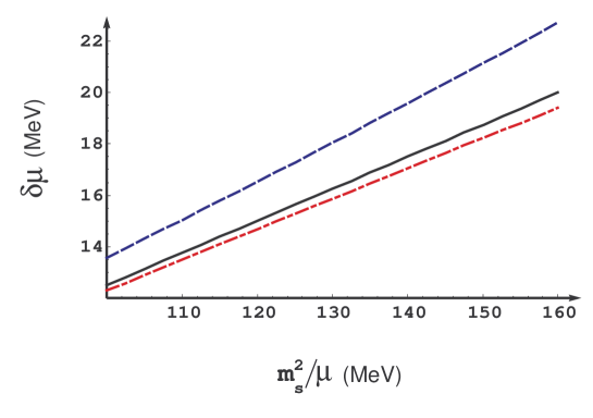
Figure 1: Quark chemical potential differences $\delta\mu_{2}$ (dashed, blue online) and $\delta\mu_{3}$ (dash-dotted, red online) together with their common value $\displaystyle\frac{m_{s}^{2}}{8\mu}$ obtained neglecting $1/\mu$ corrections (full line).

We note that the effect of introducing the $1/\mu$ correction is to induce an asymmetric splitting of the Fermi surfaces of the $s$ and $d$ with respect to the $u$ quark Fermi sphere, more exactly $\delta\mu_{2}>\delta\mu_{3}$; neglecting higher order effects, as in Casalbuoni:2005zp , one would get the result $\delta\mu_{2}=\delta\mu_{3}$ since in this limit $\displaystyle\mu_{e}=\frac{m_{s}^{2}}{4\mu}$. The results for the splitting of chemical potentials are reported in Fig. 1 (dash-dotted and dashed, respectively red and blue online) together with the result obtained in the large $\mu$ limit (continuous black line).

As a consequence of these results we expect a difference between the two gap parameters, with $\Delta_{2}<\Delta_{3}$. This is confirmed by the results of the gap equations that are reported in Fig. 2. Also in this case we report the two gaps in the new approximation (dash-dotted and dashed, respectively red and blue online) together with the result $\Delta_{2}=\Delta_{3}$ obtained in the large $\mu$ limit (continuous black line).

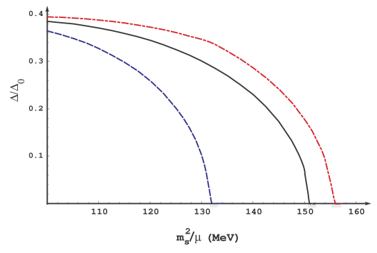
Figure 2: The full line represents the previous solution $\Delta_{2}=\Delta_{3}$; the dashed (blue online) and dash-dotted (red online) lines are respectively $\Delta_{2}$ and $\Delta_{3}$ in the new approximation. All the gap parameters are normalized to the CFL homogeneous gap $\Delta_{0}=25MeV$.

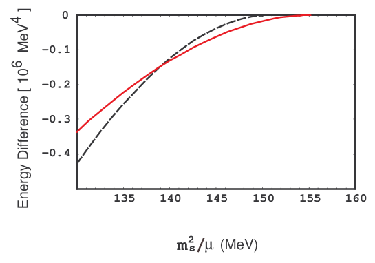
Figure 3: The free energy difference in the previous and in the present approximation (respectively dashed black line and continuous line, red online).

From these results we can compute the difference between the free energies in the LOFF state and in the normal phase. This result is reported in Fig. 3 (continuous curve, red online), together with the result of Casalbuoni:2005zp obtained neglecting $1/\mu$ corrections (dotted line).

The effect of the corrections considered in the present paper is to change the nature of the phase transitions in the LOFF regime. The LOFF has been enlarged, as it can be seen from both figs. 2 and 3. However, whereas in the previous approximation the LOFF window was characterized by one gap, and by condensation in two channels: $u-s$ and $u-d$, now we have LOFF pairing in both channels only in a tiny region, for smaller valuers of $m_{s}^{2}/\mu$, while near the end point of the superconductive region ($m_{s}^{2}/\mu>132$ MeV) only $\Delta_{3}\neq 0$ and therefore there is no $u-s$ pairing. We can call this new phase LOFF2s. It differs from the the LOFF phase with two flavors $u$ and $d$ for the presence of the strange quark, which plays an active role in modifying, by mass effects, the chemical potentials and being decisive to implement electric neutrality. The transition between the two LOFF phases is second order.

We finally note that we are not able to fix the lower end of the LOFF phase with two gaps $\Delta_{2}\neq 0$ and $\Delta_{3}\neq 0$. As a matter of fact this point would be obtained by comparing the LOFF and the gCFL free energies, which will be only feasible going beyond the existing approximation, when all the $1/\mu$ corrections in the gCFL phase are considered. In any case we expect that the LOFF phase with two gaps, in the one plane wave approximation, is limited to a narrow range of values of $m_{s}^{2}/\mu$, because, in the previous approximation, its lower end was for $m_{s}^{2}/\mu\sim 128$ MeV Casalbuoni:2005zp and LOFF2s begins at $m_{s}^{2}/\mu\sim 132$ MeV .

V Conclusions

An interesting point to be investigated is the chromomagnetic stability of the LOFF2s phase. We have applied the results of Ciminale:2006sm to this phase, characterized, as we have stressed by $\Delta_{2}=0$ and $\Delta_{3}\neq 0$ and we have found that it is chromomagnetically stable: three gluons, related to the generators of an unbroken $SU(2)_{c}$ remain massless while all the Meissner masses of the remaining gluons (both the longitudinal and transverse ones) are real, a result that is also implicit in the conclusions of refs. Giannakis:2005vw . Incidentally, since there is change of symmetry, this result shows that LOFF2s and the LOFF state with two nonvanishing gaps are distinct phases. It would be tempting to extend the analysis of stability to the tiny region with $m_{s}^{2}/\mu$ near, but smaller of $132$ MeV, and $\Delta_{2}\neq 0$, $\Delta_{3}\neq 0$. This extension is complicated by the fact that we do not know exactly where this LOFF phase extends, because a complete ${\cal O}(1/\mu)$ calculation of the gCFL has not yet been performed. We plan to come back to this problem in the future.

In conclusion we have proved the relevance of $1/\mu$ effects for the LOFF phase with three flavors in the one-plane wave approximation. Some of our results can be important also for the more complex studies with several plane waves Rajagopal:2006ig ; Rajagopal:2006dp . Since also in this case the inclusion of the $1/\mu$ contributions breaks the symmetry between $d-u$ and $u-s$ pairings, this can provide some hints on the best strategy to follow in order to identify the most favored crystalline structures. Moreover we have found that at the order $\Delta^{6}$ the color chemical potentials do not vanish, which can be also important in crystallography of three-flavor quark matter because in the GL expansion one has to take into account terms up to this order.

References

- (1) J. C. Collins and M. J. Perry, Phys. Rev. Lett. 34, 1353 (1975); B. Barrois, Nucl. Phys. B129, 390 (1977); S. Frautschi, Proceedings of workshop on hadronic matter at extreme density, Erice 1978; D. Bailin and A. Love, Phys. Rept. 107, 325 (1984).
- (2) M. G. Alford, K. Rajagopal and F. Wilczek, Phys. Lett. B 422, 247 (1998) [arXiv:hep-ph/9711395]; R. Rapp, T. Schäfer, E. V. Shuryak and M. Velkovsky, Phys. Rev. Lett. 81, 53 (1998) [arXiv:hep-ph/9711396]; D. T. Son, Phys. Rev. D 59, 094019 (1999) [arXiv:hep-ph/9812287]; R. D. Pisarski and D. H. Rischke, Phys. Rev. D 61, 074017 (2000) [arXiv:nucl-th/9910056].
- (3) K. Rajagopal and F. Wilczek, arXiv:hep-ph/0011333. M. G. Alford, Ann. Rev. Nucl. Part. Sci. 51, 131 (2001) [arXiv:hep-ph/0102047]; G. Nardulli, Riv. Nuovo Cim. 25N3, 1 (2002) [arXiv:hep-ph/0202037]; S. Reddy, Acta Phys. Polon. B 33, 4101 (2002) [arXiv:nucl-th/0211045]; T. Schafer, arXiv:hep-ph/0304281; D. H. Rischke, Prog. Part. Nucl. Phys. 52, 197 (2004) [arXiv:nucl-th/0305030]; M. Alford, Prog. Theor. Phys. Suppl. 153, 1 (2004) [arXiv:nucl-th/0312007]; M. Buballa, Phys. Rept. 407, 205 (2005) [arXiv:hep-ph/0402234]; H. c. Ren, arXiv:hep-ph/0404074; M. Huang, Int. J. Mod. Phys. E 14, 675 (2005) [arXiv:hep-ph/0409167]; I. A. Shovkovy, Found. Phys. 35, 1309 (2005) [arXiv:nucl-th/0410091]; T. Schaefer, arXiv:hep-ph/0509068.
- (4) M. G. Alford, K. Rajagopal and F. Wilczek, Nucl. Phys. B 537, 443 (1999) [arXiv:hep-ph/9804403].
- (5) I. Shovkovy and M. Huang, Phys. Lett. B 564, 205 (2003) [arXiv:hep-ph/0302142]. M. Huang and I. Shovkovy, Nucl. Phys. A 729, 835 (2003) [arXiv:hep-ph/0307273].
- (6) M. Alford, C. Kouvaris and K. Rajagopal, Phys. Rev. Lett. 92, 222001 (2004) [arXiv:hep-ph/0311286];
- (7) M. Alford, C. Kouvaris and K. Rajagopal, Phys. Rev. D 71, 054009 (2005) [arXiv:hep-ph/0406137]. K. Fukushima, C. Kouvaris and K. Rajagopal, Phys. Rev. D 71, 034002 (2005) [arXiv:hep-ph/0408322].
- (8) M. Huang and I. A. Shovkovy, Phys. Rev. D 70, 051501 (2004) [arXiv:hep-ph/0407049]. M. Huang and I. A. Shovkovy, Phys. Rev. D 70, 094030 (2004) [arXiv:hep-ph/0408268].
- (9) R. Casalbuoni, R. Gatto, M. Mannarelli, G. Nardulli and M. Ruggieri, Phys. Lett. B 605, 362 (2005) [Erratum-ibid. B 615, 297 (2005)] [arXiv:hep-ph/0410401]; K. Fukushima, Phys. Rev. D 72, 074002 (2005) [arXiv:hep-ph/0506080]; M. Alford and Q. h. Wang, J. Phys. G 31, 719 (2005) [arXiv:hep-ph/0501078]; K. Fukushima, arXiv:hep-ph/0510299.
- (10) M. Huang, Phys. Rev. D 73, 045007 (2006) [arXiv:hep-ph/0504235]; D. K. Hong, arXiv:hep-ph/0506097; M. Alford and Q. h. Wang, J. Phys. G 32, 63 (2006) [arXiv:hep-ph/0507269]; A. Kryjevski, arXiv:hep-ph/0508180; T. Schafer, arXiv:hep-ph/0508190;
- (11) E. V. Gorbar, M. Hashimoto and V. A. Miransky, Phys. Lett. B 632, 305 (2006) [arXiv:hep-ph/0507303].
- (12) I. Giannakis, D. Hou, M. Huang and H. c. Ren, arXiv:hep-ph/0606178.
- (13) M. G. Alford, J. A. Bowers and K. Rajagopal, Phys. Rev. D 63, 074016 (2001) [arXiv:hep-ph/0008208]; J. A. Bowers, J. Kundu, K. Rajagopal and E. Shuster, Phys. Rev. D 64, 014024 (2001) [arXiv:hep-ph/0101067]; A. K. Leibovich, K. Rajagopal and E. Shuster, Phys. Rev. D 64, 094005 (2001) [arXiv:hep-ph/0104073]; J. A. Bowers and K. Rajagopal, Phys. Rev. D 66, 065002 (2002) [arXiv:hep-ph/0204079]; R. Casalbuoni, M. Ciminale, M. Mannarelli, G. Nardulli, M. Ruggieri and R. Gatto, Phys. Rev. D 70, 054004 (2004) [arXiv:hep-ph/0404090].
- (14) R. Casalbuoni and G. Nardulli, Rev. Mod. Phys. 76, 263 (2004) [arXiv:hep-ph/0305069].
- (15) A. I. Larkin and Yu. N. Ovchinnikov, Zh. Eksp. Teor. Fiz. 47, 1136 (1964) (Sov. Phys. JETP 20, 762 (1965)); P.Fulde and R. A. Ferrell, Phys. Rev. 135, A550 (1964).
- (16) I. Giannakis and H. C. Ren, Phys. Lett. B 611, 137 (2005) [arXiv:hep-ph/0412015].
- (17) I. Giannakis and H. C. Ren, Nucl. Phys. B 723, 255 (2005) [arXiv:hep-th/0504053]; I. Giannakis, D. f. Hou and H. C. Ren, Phys. Lett. B 631, 16 (2005) [arXiv:hep-ph/0507306].
- (18) E. V. Gorbar, M. Hashimoto and V. A. Miransky, Phys. Rev. Lett. 96, 022005 (2006) [arXiv:hep-ph/0509334].
- (19) R. Casalbuoni, R. Gatto, N. Ippolito, G. Nardulli and M. Ruggieri, Phys. Lett. B 627, 89 (2005) [Erratum-ibid. B 634, 565 (2006)] [arXiv:hep-ph/0507247].
- (20) M. Ciminale, G. Nardulli, M. Ruggieri and R. Gatto, Phys. Lett. B 636, 317 (2006) [arXiv:hep-ph/0602180].
- (21) M. Mannarelli, K. Rajagopal and R. Sharma, arXiv:hep-ph/0603076.
- (22) K. Rajagopal and R. Sharma, arXiv:hep-ph/0605316.
- (23) K. Rajagopal and R. Sharma, arXiv:hep-ph/0606066.
- (24) D. K. Hong, Phys. Lett. B 473, 118 (2000) [arXiv:hep-ph/9812510]. D. K. Hong, Nucl. Phys. B 582, 451 (2000) [arXiv:hep-ph/9905523].
- (25) S. R. Beane, P. F. Bedaque and M. J. Savage, Phys. Lett. B 483, 131 (2000) [arXiv:hep-ph/0002209].
- (26) R. Casalbuoni, R. Gatto, G. Nardulli and M. Ruggieri, Phys. Rev. D 68, 034024 (2003) [arXiv:hep-ph/0302077].