The linear sigma model at a finite isospin chemical potential

Abstract

The effect of finite isospin chemical potential to the effective masses of the mesons at finite temperature is investigated in the framework of the $O(4)$ linear sigma model with explicit chiral symmetry breaking. We present a mechanism to include the isospin chemical potential in the model. By using the Cornwall-Jackiw-Tomboulis method of composite operators, we obtain a set gap equations for the effective masses of the mesons and get the numerical results in the Hartree approximation. We find that the introduction of the chemical potential only affects the mass of the charged pions and sigma, while there is almost NO effects on the mass of neutral pions.

I Introduction

Nowadays, it is widely believed that QCD is the most promising theory to explain the strong interactions. However, due the property of confinement and asymptotic freedom we can accept and study the quarks as free only at very high energies. This much expected phase, which is called Quark Gluon Plasma (QGP), is under investigation in RHIC experiments and there is strong evidence that it has been observed. According to Heinz Heinz:2004pj it seems that elliptic flow at high enough collision energies is a QGP signature. The recent results from RHIC experiments have attracted many attempts for theoretical models to be testedRischke:2003mt . Recently there are also a lot of attempts to study the phases of QCD from first principles using lattice techniques at finite baryon density and chemical isospin potential. There is, however, an alternative approach which applies only in the low energy regime. Following this path, it is necessary to use a variety of effective phenomenological models and QCD–like theories in order to mimic some of the features of QCD.

A quite popular model, which fulfils these requirements, exhibiting many of the symmetries observed in QCD, is the linear sigma model. The model was first introduced in the 1960s as a model for pion–nucleon interactions Gell-Mann:1960np and has attracted much attention recently, especially in studies involving disoriented chiral condensates Rajagopal:1992qz ; Rajagopal:1993ah ; Kuraev:2003tr . The linear sigma model with a $U(N_{f})\times U(N_{f})$ symmetry and two to four quark flavors have been studied in the Hartree-Fock or Hartree approximationPetropoulos:1998gt ; Lenaghan:2000ey ; Roder:2003uz ; Petropoulos:2004bt within the Cornwall–Jackiw–Tomboulis (CJT) formalismAmelino-Camelia:1992nc , and the large-N approximation of the linear sigma model has been investigated by using the same formlism in RefsAmelino-Camelia:1997dd ; Lenaghan:1999si ; Nemoto:1999qf . Within the same framework, Shu and Li Shu:2005bj have studied Bose-Einstein condensation and the chiral phase transition in the chiral limit, and they introduced the chemical potential through the third component of isospin charge. In this discussion, we apply a mechanism Kogut:1999iv ; Kogut:2000ek ; Son:2000xc to include the isospin chemical potential in the linear sigma model, then by using CJT method, we study the chiral phase transition at finite isospin chemical potential in explicit chiral symmetry breaking.

The organization of this paper is as follows. In the next section we present the basics about the linear sigma model and how this model incorporates some of the basic features of QCD, then we introduce the isospin chemical potential in the model. In Section III we calculate the effective potential of the model by using the Cornwall–Jackiw–Tomboulis method of composite operators and obtain a set of gap equations for the thermal effective mass of the pions. The solution of these gap equations is presented in Section IV. In the last section we present our conclusions.

II The Model

Consider an idealisation of QCD with two species of massless quarks $u$ and $d$. The Lagrangian of strong interaction physics is invariant under $SU(2)_{L}\times SU(2)_{R}$ chiral transformation

$$\Psi_{L,R}\rightarrow\exp(-i\vec{\theta}_{L,R}\cdot\vec{\tau})\Psi_{L,R},$$ (1)

where $\Psi_{L,R}=(u,d)_{L,R}$. However this chiral symmetry does not appear in the low energy particle spectrum since it is spontaneously broken. Consequently, three Goldstone bosons, the pions, appear and the (constituent) quarks become massive. At low energy, the spontaneous breaking of chiral symmetry can be described by an effective theory, the linear sigma model, which involves the massless pions $\vec{\pi}$ and a massive $\sigma$ particle. Here, the $\sigma$ field can be used to represent the quark condensate which is considered as the order parameter of the chiral phase transition. This choice is a natural one since both exhibit the same behaviour under chiral transformations. The pions are very light particles and can be considered approximately as massless Goldstone bosons.

There are different ways to write down the Lagrangian of the linear sigma model and each with certain advantages and disadvantages. One version which demonstrates the chiral properties of this Lagrangian in a straightforward way involves the introduction of a matrix field $\Phi$ defined as

$$\Phi=\sigma\frac{\tau^{0}}{2}+i\vec{\pi}\cdot\frac{\vec{\tau}}{2}~{},$$ (2)

where $\tau^{0}$ is the unity matrix and $\vec{\tau}=(\tau_{1},\tau_{2},\tau_{3})$ are the Pauli matrix. This matrix field satisfies the normalization condition $Tr(\tau^{a}\tau^{b})=2\delta^{ab}$. Under $SU(2)_{L}\times SU(2)_{R}$ chiral transformations, $\Phi$ transforms as

$$\Phi\rightarrow L^{+}\Phi R~{}.$$ (3)

Using this parametrisation the renormalizable effective Lagrangian of the linear sigma model can be written as Itzykson:1980rh Donoghue:1992dd

$${\mathcal{L}}_{0}={\mathcal{L}}_{\Phi}+{\mathcal{L}}_{q}~{},$$ (4)

where

$${\mathcal{L}}_{\Phi}=\textrm{Tr}[(\partial_{\mu}\Phi)^{+}(\partial^{\mu}\Phi)]-m^{2}\textrm{Tr}(\Phi^{+}\Phi)-\frac{\lambda}{6}[\textrm{Tr}(\Phi^{+}\Phi)]^{2}~{}$$ (5)

$${\mathcal{L}}_{q}=\overline{\Psi}_{L}i\gamma^{\mu}\partial_{\mu}\Psi_{L}+\overline{\Psi}_{R}i\gamma^{\mu}\partial_{\mu}\Psi_{R}-2g\overline{\Psi}_{L}\Phi\Psi_{R}+h.c..$$ (6)

When chiral symmetry is breaking, the field $\sigma$ acquires a non–vanishing vacuum expectation value, which breaks $SU(2)_{L}\times SU(2)_{R}$ down to $SU(2)_{L+R}$. It results in a massive sigma particle $\sigma$ and three massless Goldstone bosons $\vec{\pi}$, as well as giving a mass $m_{q}=gf_{\pi}$ to the constituent quarks.

Now let us consider the Lagrangian of the linear sigma model for two massless quarks of flavors $u$, $d$ with different chemical potential $\mu_{u}$ and $\mu_{d}$,

$${\mathcal{L}}^{\prime}={\mathcal{L}}_{0}+{\mathcal{L}}_{\mu}={\mathcal{L}}_{\Phi}+{\mathcal{L}}_{q}+\Psi_{L}^{\dagger}B\Psi_{L}+\Psi_{R}^{\dagger}B\Psi_{R},$$ (7)

where $B=\left(\begin{array}[]{c}\mu_{u}\\ 0\end{array}\begin{array}[]{c}0\\ \mu_{d}\end{array}\right)$ is the matrix of chemical potentials. The term ${\mathcal{L}}_{\mu}$ can be expressed either by the variables $\mu_{u}$, $\mu_{d}$ or by the two combinations $\mu_{B}=\frac{1}{2}(\mu_{u}+\mu_{d})$ and $\mu_{I}=\frac{1}{2}(\mu_{u}-\mu_{d})$, which couple to the baryon charge density and the third component of isospin respectively. Then we have

$${\mathcal{L}}_{\mu}=\mu_{B}(\Psi^{{\dagger}}_{L}\Psi_{L}+\Psi^{{\dagger}}_{R}\Psi_{R})+\mu_{I}(\Psi^{{\dagger}}_{L}\tau_{3}\Psi_{L}+\Psi^{{\dagger}}_{R}\tau_{3}\Psi_{R})~{}.$$ (8)

Both ${\mathcal{L}}_{\Phi}$ and ${\mathcal{L}}_{q}$ are $SU(2)_{L}\times SU(2)_{R}$ invariant, but the symmetry is reduced by the baryon charge density term $\mu_{B}(\Psi^{{\dagger}}_{L}\Psi_{L}+\Psi^{{\dagger}}_{R}\Psi_{R})$ to $SU(2)_{L+R}$ and further reduced by the isospin term $\mu_{I}(\Psi^{{\dagger}}_{L}\tau_{3}\Psi_{L}+\Psi^{{\dagger}}_{R}\tau_{3}\Psi_{R})$ to $U(1)_{L+R}$. In what follows, we consider an idealized case where $\mu_{I}$ is nonzero while $\mu_{B}=0$. A similar choice is adopted in Refs.Son:2000xc Barducci:2004tt . According to their analysis such an approximation is justified by the fact that we are dealing with the dynamics of strong interactions. In any realistic setting, $\mu_{I}\ll\mu_{B}$. Such a system is unstable due to weak decays which do not conserve isospin. However, we can still imagine that all relatively slow electroweak effects are turned off.

We note that the effects of the isospin chemical potential $\mu_{I}$ can be included to the Lagrangian of the linear sigma model without additional phenomenological parameters by promoting $SU(2)_{L}\times SU(2)_{R}$ to a local gauge symmetry and viewing $\mu_{I}$ as the zeroth component of a gauge potential Kogut:1999iv ; Kogut:2000ek ; Son:2000xc . This means that we can rewrite the terms ${\mathcal{L}}_{q}+{\mathcal{L}}_{\mu}$ as

$${\mathcal{L}}_{q}^{\prime}=\bar{\Psi}_{L}i\gamma^{\mu}D_{\mu}\Psi_{L}+\bar{\Psi}_{R}i\gamma^{\mu}D_{\mu}\Psi_{R}~{},$$ (9)

where $D_{\mu}=\partial_{\mu}-i\mu_{I}A_{\mu}$, $A_{\mu}=A_{\mu}^{a}T^{a}$ and $T_{a}=\frac{\tau^{a}}{2}(a=1,2,3)$. Here the gauge fields $A_{\mu}$ have the following properties: $A^{3}_{0}={\mathbf{1}},A^{1}_{0}=A^{2}_{0}=0$ and $A_{i}=0$ for $i=1,2,3$. Then the term ${\mathcal{L}}_{q}^{\prime}$ is invariant under the $SU(2)_{L}\times SU(2)_{R}$ local transformations:

$$\Psi_{L,R}\rightarrow U\Psi_{L,R},U=\exp(-i\vec{\theta}_{L,R}(x)\cdot\vec{T})~{}.$$ (10)

However, the term ${\mathcal{L}}_{\Phi}$ is not invariant under $SU(2)_{L}\times SU(2)_{R}$ local transformations. In order to ensure the effective Lagrangian of the linear sigma model is also invariant under this local symmetry we have to replace the derivatives in Eq. (5) by the covariant derivatives:

$${\mathcal{L}}_{\Phi}=\textrm{Tr}[(D_{\mu}\Phi)^{+}(D_{\mu}\Phi)]-m^{2}\textrm{Tr}(\Phi^{+}\Phi)-\frac{\lambda}{6}(\textrm{Tr}(\Phi^{+}\Phi))^{2}~{},$$ (11)

where the covariant derivatives are defined as:

$$D_{0}\Phi = \partial_{0}\Phi-i\mu_{I}(\frac{\tau^{3}}{2}\Phi-\Phi\frac{\tau^{3}}{2})$$ (12)

$$D_{i}\Phi = \partial_{i}\Phi,(i=1,2,3)~{}.$$ (13)

Thus the gauge invariance fixes the way $\mu_{I}$ enters the mesonic sector of the effective Lagrangian of the linear sigma model.

In order to study the effects of the finite chemical potential $\mu_{I}$ in the linear sigma model at finite temperature, we only consider the term ${\mathcal{L}}_{\Phi}$ neglecting the fermion fields. It is convenient to define the new fields:

$$\pi^{\pm}=\frac{\pi^{1}\pm i\pi^{2}}{\sqrt{2}}~{}.$$ (14)

The Lagrangian ${\mathcal{L}}_{\Phi}$ now can be expressed as

$${\mathcal{L}}=\frac{1}{2}(\partial_{\mu}\sigma)(\partial^{\mu}\sigma)+\frac{1}{2}(\partial_{\mu}\pi^{0})(\partial^{\mu}\pi^{0})+(D_{\mu}\pi)^{+}(D^{\mu}\pi)^{-}-V(\sigma,\vec{\pi})~{},$$ (15)

where the potential is

$$V(\sigma,\vec{\pi})=\frac{m^{2}}{2}(\sigma^{2}+\vec{\pi}^{2})+\frac{\lambda}{24}(\sigma^{2}+\vec{\pi}^{2})^{2}~{},$$ (16)

and $(D_{0}\pi)^{\pm}=(\partial_{0}\pm i\mu_{I})\pi^{\pm}$, $(D_{i}\pi)^{\pm}=\partial_{i}\pi^{\pm}$ for $(i=1,2,3)$.

The $SU(2)_{L}\times SU(2)_{R}$ symmetry of the linear sigma model is explicitly broken if the potential $V(\sigma,\vec{\pi})$ is made slightly asymmetric by adding to the basic Lagrangian in Eq. (4) a term of form

$${\mathcal{L}}_{b}=\epsilon\sigma~{}.$$ (17)

With this addition, the vector isospin $SU(2)$ symmetry remains exact, but the axial $SU(2)$ transformation is no longer invariant. The potential now has the form

$$V(\sigma,\vec{\pi})=\frac{m^{2}}{2}(\sigma^{2}+\vec{\pi}^{2})+\frac{\lambda}{24}(\sigma^{2}+\vec{\pi}^{2})^{2}-\epsilon\sigma~{}.$$ (18)

To the leading order in $\epsilon$, this shifts the minimum of the potential to $v=f_{\pi}+\frac{3\epsilon}{\lambda f_{\pi}^{2}}$, and as a result the pions acquire mass $m^{2}_{\pi}=\frac{\epsilon}{f_{\pi}}$.

At tree level and zero temperature the parameters of the Lagrangian are fixed in a way that these masses agree with the observed value of pion mass $m_{\pi}=138$ MeV and the most commonly accepted value for sigma mass $m_{\sigma}=600$ MeV. Then, the coupling constant $\lambda$ of the model can be related to zero temperature properties of the pions and sigma through the expression

$$\lambda=\frac{3(m^{2}_{\sigma}-m^{2}_{\pi})}{f^{2}_{\pi}}~{},$$ (19)

where $f_{\pi}\approx 93$ MeV is the pion decay constant. The negative mass parameter $m^{2}$ is introduced in order to ensure spontaneous breaking of symmetry and its value is chosen to be

$$-m^{2}=(m^{2}_{\sigma}-3m^{2}_{\pi})/2>0~{}.$$ (20)

III The CJT effective potential

In this section we calculate the finite temperature effective potential for the linear sigma model at finite isospin chemical potential. In our calculations we use the imaginary time formalism, which is also known as the Matsubara formalismDolan:1973qd ; Kapusta:1989 ; LeBellac:1996 ; Das:1997gg . This means that in the case of Bosons, we have

$$\int\frac{d^{4}k}{(2\pi)^{4}}f(k)\rightarrow\frac{1}{\beta}\sum_{n}\int\frac{d^{3}\vec{k}}{(2\pi)^{3}}f(i\omega_{n},\vec{k})\equiv\int_{\beta}f(i\omega_{n},\vec{k}),$$

where $\beta$ is the inverse temperature, $\beta=\frac{1}{k_{B}T}$, and as usual Boltzmann’s constant is taken as $k_{B}=1$, and $\omega_{n}=2\pi nT$, $n=0,\pm 1,\pm 2,\pm 3,\ldots$ For simplicity we have introduced a subscript $\beta$ to denote integration and summation over the Matsubara frequency sums.

The starting point is the Lagrangian given in Eq. (15) with the choice of the asymmetric potential given in Eq. (18). By shifting the sigma field as $\sigma\rightarrow\sigma+\phi$ the classical potential takes the form

$$U(\phi)=\frac{1}{2}m^{2}\phi^{2}+\frac{\lambda}{24}\phi^{4}-\epsilon\phi.$$ (21)

The tree-level sigma and pion propagators corresponding to the above Lagrangian have the form

$$D_{\sigma}^{-1} = \omega_{n}^{2}+\vec{k}^{2}+m^{2}+\frac{1}{2}\lambda\phi^{2},$$ (22a)

$$D_{0}^{-1} = \omega_{n}^{2}+\vec{k}^{2}+m^{2}+\frac{1}{6}\lambda\phi^{2},$$ (22b)

$$D^{-1}_{c} = (\omega_{n}+i\mu_{I})^{2}+\vec{k}^{2}+m^{2}+\frac{1}{6}\lambda\phi^{2}.$$ (22c)

Eq.(22c) represents the inverse propagator of $\pi_{+}$ and $\pi_{-}$ due to the facts that $\omega_{n}+i\mu_{I}$ and $\omega_{n}-i\mu_{I}$ are equivalent in describing the propagators of $\pi_{+}$ and $\pi_{-}$Shu:2005bj .

The interaction Lagrangian which describes the vertices of the shifted theory is given by

$${\mathcal{L}}_{int}=-\frac{\lambda}{12}\sigma^{2}\vec{\pi}^{2}-\frac{\lambda}{24}\sigma^{4}-\frac{\lambda}{24}\vec{\pi}^{4}-\frac{\lambda}{6}\phi\sigma\vec{\pi}^{2}-\frac{\lambda}{6}\phi\sigma^{3}~{}.$$ (23)

Here, we omit the constants and the terms linear in the $\sigma$ fields for simplicity. In our approximation we do not consider interactions which are given by the last two terms in the above Lagrangian.

Figure 1: Two–particle irreducible graphs which contribute to the effective potential of a $\lambda\phi^{4}$ theory in the CJT method up to the three-loop level. The solid line represents the dressed propagator $G(x,y)$. There are two kinds of vertices: a three-particle vertex and a four-particle vertex.

Then, for constant $\phi$, according to CJT formalism Amelino-Camelia:1992nc the finite temperature effective potential for $\lambda\phi^{4}$ theory is given by

$$V(\phi,G) = U(\phi)+\frac{1}{2}\int_{\beta}\ln G^{-1}(\phi;k)$$ (24)

$$+\frac{1}{2}\int_{\beta}[D^{-1}(\phi;k)G(\phi;k)-1]$$

$$+V_{2}(\phi,G).$$

Here, $G(\phi;k)$ denotes the full propagator of the theory and we have introduced a shorthand notation for the space integration and summation over the bosonic Matsubara frequencies so the symbol $\int_{\beta}$ stands for $T\sum_{n}\int d^{3}\vec{k}/(2\pi)^{3}$. The last term $V_{2}(\phi,G)$ represents the sum of all two and higher–order loop two–particle irreducible vacuum graphs of the theory with vertices given by ${\mathcal{L}}_{int}$ and propagators set equal to $G(\phi;k)$. The diagrams contributing to $V_{2}(\phi,G)$ for $\lambda\phi^{4}$ theory are shown in Fig. 1. Evaluating the effective potential in Hartree approximation means that one needs to take into account the ”$\infty$” type diagram only. In the case of $\lambda\phi^{4}$ theory this diagram is the leading order in $V_{2}(\phi,G)$ in both the loop expansion and the $1/N$ expansion. We adopt this approximation in the case of the linear sigma model as well. The Hartree and large N approximations at zero chemical potential have been studied previously in Refs.Petropoulos:1998gt ; Lenaghan:2000ey ; Roder:2003uz ; Petropoulos:2004bt ; Amelino-Camelia:1997dd ; Lenaghan:1999si ; Nemoto:1999qf .

Generalising this result to finite isospin chemical potential, we derive the following expression for the effective potential at finite temperature

$$V(\phi,G) = U(\phi)+\frac{1}{2}\int_{\beta}\ln G^{-1}_{\sigma}(\phi;k)+\frac{1}{2}\int_{\beta}\ln G^{-1}_{0}(\phi;k)+\int_{\beta}\ln G^{-1}_{c}(\phi;k)$$ (25)

$$+\frac{1}{2}\int_{\beta}[D^{-1}_{\sigma}(\phi;k)G_{\sigma}(\phi;k)-1]+\frac{1}{2}\int_{\beta}[D^{-1}_{0}(\phi;k)G_{0}(\phi;k)-1]$$

$$+\int_{\beta}[D^{-1}_{c}(\phi;k)G_{c}(\phi;k)-1]+V_{2}(\phi,G_{\sigma},G_{0},G_{c}).$$

The first term $U(\phi)$ on the right handside is the classical potential and the last term $V_{2}(\phi,G_{\sigma},G_{0},G_{c})$ denotes the contribution from two–particle irreducible diagrams. In the following we include only the two–loop diagrams shown in Fig. 2. These contribute the following terms in the potential

$$V_{2}(\phi,G_{\sigma},G_{\pi^{0}},G_{c}) = 3\frac{\lambda}{24}\left[\int_{\beta}G_{\sigma}^{-1}(\phi;k)\right]^{2}+2\frac{\lambda}{24}\left[\int_{\beta}G_{\sigma}^{-1}(\phi;k)\right]\left[\int_{\beta}G_{0}^{-1}(\phi;k)\right]$$ (26)

$$+4\frac{\lambda}{24}\left[\int_{\beta}G_{\sigma}^{-1}(\phi;k)\right]\left[\int_{\beta}G^{-1}_{c}(\phi;k)\right]+4\frac{\lambda}{24}\left[\int_{\beta}G_{0}^{-1}(\phi;k)\right]\left[\int_{\beta}G_{c}^{-1}(\phi;k)\right]$$

$$+3\frac{\lambda}{24}\left[\int_{\beta}G_{0}^{-1}(\phi;k)\right]^{2}+8\frac{\lambda}{24}\left[\int_{\beta}G_{c}^{-1}(\phi;k)\right]^{2}.$$

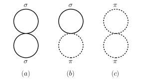
Figure 2: The Hartree contributions to the CJT effective potential. Solid lines correspond to $G_{\sigma}$, while dashed lines correspond to $G_{\pi}$.

Minimizing the effective potential with respect to full propagators we obtain the following system of nonlinear gap equations:

$$G_{\sigma}^{-1} = D_{\sigma}^{-1}+\frac{\lambda}{2}\int_{\beta}G_{\sigma}(\phi;k)+\frac{\lambda}{6}\int_{\beta}G_{0}(\phi;k)+\frac{\lambda}{3}\int_{\beta}G_{c}(\phi;k),$$ (27a)

$$G_{0}^{-1} = D_{0}^{-1}+\frac{\lambda}{6}\int_{\beta}G_{\sigma}(\phi;k)+\frac{\lambda}{2}\int_{\beta}G_{0}(\phi;k)+\frac{\lambda}{3}\int_{\beta}G_{c}(\phi;k),$$ (27b)

$$G^{-1}_{c} = D^{-1}+\frac{\lambda}{6}\int_{\beta}G_{\sigma}(\phi;k)+\frac{\lambda}{6}\int_{\beta}G_{0}(\phi;k)+\frac{2\lambda}{3}\int_{\beta}G_{c}(\phi;k).$$ (27c)

In order to proceed we can make the following ansatz for the full propagators:

$$G_{\sigma}^{-1} = \omega_{n}^{2}+\vec{k}^{2}+M^{2}_{\sigma},$$

$$G_{0}^{-1} = \omega_{n}^{2}+\vec{k}^{2}+M^{2}_{0},$$

$$G^{-1}_{c} = (\omega_{n}+i\mu_{I})^{2}+\vec{k}^{2}+M_{c}^{2},$$

where $M_{\sigma}$, $M_{0}$ and $M_{c}$ are the effective masses of $\sigma$ meson, $\pi_{0}$ and charged pion dressed by interaction contributions from the diagrams of Fig.2. The dressed sigma and pion masses are then determined by the following gap equations:

$$M_{\sigma}^{2} = m^{2}+\frac{\lambda}{2}\phi^{2}+\frac{\lambda}{2}F(M_{\sigma})+\frac{\lambda}{6}F(M_{0})+\frac{\lambda}{3}F(M_{c}),$$ (28a)

$$M_{0}^{2} = m^{2}+\frac{\lambda}{6}\phi^{2}+\frac{\lambda}{6}F(M_{\sigma})+\frac{\lambda}{2}F(M_{0})+\frac{\lambda}{3}F(M_{c}),$$ (28b)

$$M_{c}^{2} = m^{2}+\frac{\lambda}{6}\phi^{2}+\frac{\lambda}{6}F(M_{\sigma})+\frac{\lambda}{6}F(M_{0})+\frac{2\lambda}{3}F(M_{c}).$$ (28c)

Here we have used a shorthand notation and introduced the function

$$F(M_{\sigma}) = \int_{\beta}\frac{1}{\omega_{n}^{2}+\vec{k}^{2}+M^{2}_{\sigma}},$$ (29a)

$$F(M_{0}) = \int_{\beta}\frac{1}{\omega_{n}^{2}+\vec{k}^{2}+M^{2}_{0}},$$ (29b)

$$F(M_{c}) = \int_{\beta}\frac{1}{(\omega_{n}+i\mu_{I})^{2}+\vec{k}^{2}+M_{c}^{2}}.$$ (29c)

At the level of the Hartree approximation, the thermal effective masses are independent of momentum and are functions of the order parameter $\phi$ and the temperature $T$. Moreover, in our case it is also function of the finite isospin chemical potential $\mu_{I}$.

In terms of the solutions of the gap equations (28), the effective potential at finite temperature can be written in the form

$$V(\phi,M) = \frac{1}{2}m^{2}\phi^{2}+\frac{\lambda}{24}\phi^{4}-\epsilon\phi+\frac{1}{2}\int_{\beta}\ln G_{\sigma}^{-1}+\frac{1}{2}\int_{\beta}\ln G_{0}^{-1}+\int_{\beta}\ln G_{c}^{-1}$$ (30)

$$-\frac{1}{2}(M_{\sigma}^{2}-m^{2}-\frac{1}{2}\lambda\phi^{2})F(M_{\sigma})-\frac{1}{2}(M_{0}^{2}-m^{2}-\frac{1}{6}\lambda\phi^{2})F(M_{0})$$

$$-(M_{c}^{2}-m^{2}-\frac{1}{6}\lambda\phi^{2})F(M_{c})+\frac{\lambda}{8}[F(M_{\sigma})]^{2}+\frac{\lambda}{8}[F(M_{0})]^{2}+\frac{\lambda}{3}[F(M_{c})]^{2}$$

$$+\frac{\lambda}{12}F(M_{\sigma})F(M_{0})+\frac{\lambda}{6}F(M_{\sigma})F(M_{c})+\frac{\lambda}{6}F(M_{0})F(M_{c}).$$

In above expression and in following discussions, we have taken the symbols $M_{\sigma}$, $M_{0}$ and $M_{c}$ just as the solutions of the gap equations (28) for simplicity.

Minimizing the effective potential with respect to the full propagators, we have found the set of nonlinear equations for the effective particles masses which are given by Eq. (28). In addition, by minimizing the potential with respect to the order parameter $\phi$ we obtain one more equation

$$[m^{2}+\frac{\lambda}{6}\phi^{2}+\frac{\lambda}{2}F(M_{\sigma})+\frac{\lambda}{6}F(M_{0})+\frac{\lambda}{3}F(M_{c})]\phi-\epsilon=0.$$ (31)

Performing the Matsubara frequency sums as in Ref.Dolan:1973qd , the logarithmic integral which appears in the above expression for the effective potential Eq. (30) divides into two parts. A zero–temperature part $Q_{0}(M)$ which is divergent and a finite–temperature part $Q_{\beta}(M)$ which is finite. For $S=M_{\sigma},M_{0}$, we have

$$Q(S) = \frac{1}{2}\int_{\beta}\ln(\omega_{n}^{2}+\vec{k}^{2}+S^{2})$$ (32)

$$= Q_{0}(S)+Q_{\beta}(S)$$

$$= \int\frac{d^{3}\vec{k}}{(2\pi)^{3}}\frac{\omega_{\vec{k}}}{2}+\frac{1}{\beta}\int\frac{d^{3}\vec{k}}{(2\pi)^{3}}\ln[1-e^{-\beta\omega_{\vec{k}}}]~{},$$

where $\omega_{\vec{k}}=\sqrt{(\vec{k}^{2}+S^{2})}$. For $S=M_{c}$, we get

$$Q(S) = \int_{\beta}\ln((\omega_{n}+i\mu_{I})^{2}+\vec{k}^{2}+S^{2})$$ (33)

$$= Q_{0}(S)+Q_{\beta}(S)$$

$$= \int\frac{d^{3}\vec{k}}{(2\pi)^{3}}\frac{\omega_{\vec{k}}}{2}+\frac{1}{\beta}\int\frac{d^{3}\vec{k}}{(2\pi)^{3}}[\ln(1-e^{-\beta(\omega_{\vec{k}}+\mu_{I})}+\ln(1-e^{-\beta(\omega_{\vec{k}}-\mu_{I})}],$$

Similarly, the second type of integral in Eq. (29) is divided into a zero–temperature part $F_{0}(M)$ and a finite-temperature part $F_{\beta}(M)$. For $S=M_{\sigma},M_{0}$, we have

$$F(S) = \int_{\beta}\frac{1}{\omega_{n}^{2}+\vec{k}^{2}+S^{2}}$$ (34)

$$= F_{0}(S)+F_{\beta}(S)$$

$$= \int\frac{d^{3}\vec{k}}{(2\pi)^{3}}\frac{1}{2\omega_{\vec{k}}}+\int\frac{d^{3}\vec{k}}{(2\pi)^{3}}\frac{1}{\omega_{\vec{k}}}\frac{1}{e^{\beta\omega_{\vec{k}}}-1}~{}.$$

And for $S=M_{c}$, we get

$$F(S) = \int_{\beta}\frac{1}{(\omega_{n}+i\mu_{I})^{2}+\vec{k}^{2}+S^{2}}$$ (35)

$$= F_{0}(S)+F_{\beta}(S)$$

$$= \int\frac{d^{3}\vec{k}}{(2\pi)^{3}}\frac{1}{2\omega_{\vec{k}}}+\int\frac{d^{3}\vec{k}}{(2\pi)^{3}}\frac{1}{2\omega_{\vec{k}}}\left[\frac{1}{e^{\beta(\omega_{\vec{k}}+\mu_{I})}-1}+\frac{1}{e^{\beta(\omega_{\vec{k}}-\mu_{I})}-1}\right].$$

The second term vanishes at zero temperature while the first term survives, but the evaluation of the integrals in Eqs. (32)(33)(34) and (35) requires renormalization. Renormalisation in many–body approximation schemes is a nontrivial procedure, but in the case of linear sigma model it has been shown by Rischke and Lenaghan Lenaghan:1999si ; Lenaghan:2000ey , that at least in the Hartree approximation the results are not affected qualitatively. We therefore simply drop the divergent terms and keep only the finite temperature part of the integrals. A similar procedure has been adopted in a number of other investigations using the linear sigma model Petropoulos:2004bt .

Using the above definitions of the integrals in Eqs. (32)(33)(34) and (35), we can rewrite the finite temperature effective potential given in Eq. (30) in a more compact form

$$V(\phi,M) = \frac{1}{2}m^{2}\phi^{2}+\frac{\lambda}{24}\phi^{4}-\epsilon\phi+Q_{\beta}(M_{\sigma})+Q_{\beta}(M_{0})+Q_{\beta}(M_{c})$$ (36)

$$-\frac{\lambda}{8}[F_{\beta}(M_{\sigma})]^{2}-\frac{\lambda}{8}[F_{\beta}(M_{0})]^{2}-\frac{\lambda}{3}[F_{\beta}(M_{c})]^{2}-\frac{\lambda}{12}F_{\beta}(M_{\sigma})F_{\beta}(M_{0})$$

$$-\frac{\lambda}{6}F_{\beta}(M_{\sigma})F_{\beta}(M_{c})-\frac{\lambda}{6}F_{\beta}(M_{0})F_{\beta}(M_{c}).$$

This final expression contains only terms which are finite.

IV Numerical results in the Hartree approximation

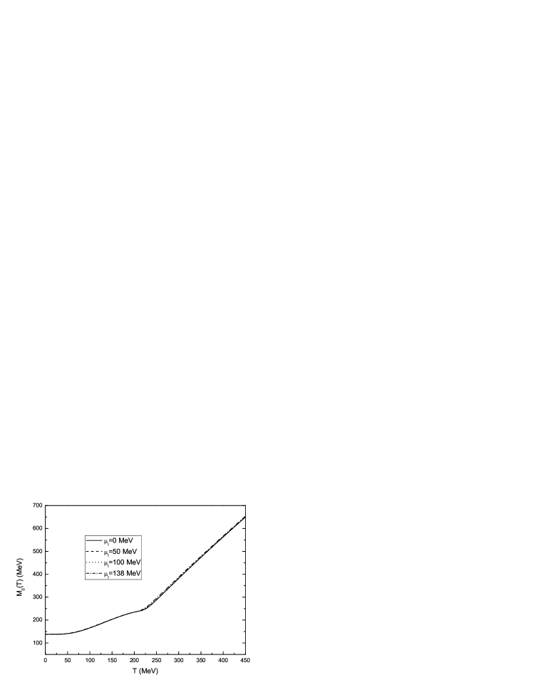
Figure 3: Solution of the system of gap equations in the case of $\epsilon\neq 0$. The effective masse of the neutral pion $M_{0}$ as a function of $T$ corresponding to $\mu_{I}=0\mathrm{MeV}$, $\mu_{I}=50\mathrm{MeV}$, $\mu_{I}=100\mathrm{MeV}$ and $\mu_{I}=138\mathrm{MeV}$ respectively.

Figure 4: Solution of the system of gap equations in the case of $\epsilon\neq 0$. The effective masse of the charged pion $M_{c}$ as a function of $T$ corresponding to $\mu_{I}=0\mathrm{MeV}$, $\mu_{I}=50\mathrm{MeV}$, $\mu_{I}=100\mathrm{MeV}$ and $\mu_{I}=138\mathrm{MeV}$ respectively.

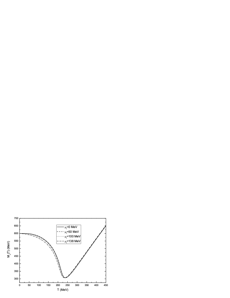
Figure 5: Solution of the system of gap equations in the case of $\epsilon\neq 0$. The effective mass of sigma $M_{\sigma}$ as a function of $T$ corresponding to $\mu_{I}=0\mathrm{MeV}$, $\mu_{I}=50\mathrm{MeV}$, $\mu_{I}=100\mathrm{MeV}$ and $\mu_{I}=138\mathrm{MeV}$ respectively.

We have solved the system of Eqs.(28) and (31) using a numerical method based on the Newton–Raphson method of solving nonlinear equations. In this way, we are able to determine the effective masses $M_{\sigma}$, $M_{0}$, $M_{c}$ and the order parameter $\phi$ as functions of $\mu_{I}$ and $T$. We are interested in both negative and positive $\mu_{I}$. The critical isospin chemical potential at zero temperature is defined by $\mu_{I}^{c}=m_{\pi}=138\mathrm{MeV}$. At $T=0$, for $|\mu_{I}|\leq m_{\pi}$, the system is in the same ground state as that at $\mu_{I}=0$. However while it is favorable to have a nontrivial vacuum which is characterized by the appearance of a condensate $<\pi^{+}>$ or $<\pi^{-}>$ when $|\mu_{I}|$ exceeds $m_{\pi}$ Son:2000xc ; Loewe:2002tw ; Loewe:2004mu . Since in this work, we only consider the effects of the isospin chemical potential on the masses of mesons and do not discuss the pion condensate Son:2000xc ; Loewe:2002tw ; Loewe:2004mu or the pion superfluidityHe:2005nk , we constrain our discussion to the values of $\mu_{I}\leq 138\mathrm{MeV}$.

We show in Fig.3, Fig.4 and Fig.5 the effective masses of the mesons $M_{0}$, $M_{c}$ and $M_{\sigma}$ as functions of $T$ corresponding to $\mu_{I}=0\mathrm{MeV}$, $\mu_{I}=50\mathrm{MeV}$, $\mu_{I}=100\mathrm{MeV}$ and $\mu_{I}=138\mathrm{MeV}$ respectively. For $\mu_{I}=0\mathrm{MeV}$, at finite $T$ we reproduce the well known results for the effective masses $M_{0}$, $M_{c}$ and $M_{\sigma}$, i.e., see RefsPetropoulos:2004bt . For $\mu_{I}\neq 0\mathrm{MeV}$, the behaviors of the meson masses at finite $T$ are very similar to the case of $\mu_{I}=0\mathrm{MeV}$. At low temperature, the pions appear with the observed mass, but their masses increase with temperature while the sigma mass decreases with temperature. At high temperature(higher than $\sim 300$ MeV), due to interactions in the thermal bath, the interactions in the thermal bath, all particles (pions and sigma) appear to have the same effective mass. At $T=0\mathrm{MeV}$, the masses of the pions and sigma particle remain constant for different $\mu_{I}$ .

In Fig.3, the results for neutral pions at various finite isospin chemical potential are nearly identical to each other. This means that the finite isospin chemical potential $\mu_{I}$ almost can not affect the effective masses of these particle duo to the fact that the neutral pions do not contribute to the finite isospin chemical potential $\mu_{I}$. However, from Eq.(22c), for a non-vanishing isospin chemical potential, the masses of the charged pions at the tree level will acquire a nontrivial isospin chemical potential dependence for finite values of temperature. In Fig.4, as the temperature increases, the effective mass of the charged pions at finite temperature changes considerably for different values of the isospin chemical potential, especially at the range of $T=50\sim 300MeV$. Moreover, from Fig.3 and Fig.4, for a certain temperature region, the masses of pions (both charged pion and neutral pion)increase with the increase of the isospin chemical potential $\mu_{I}$, though the mass of the neutral pion changes very slightly.

In Fig.5, the results for sigma particle are very difference from the poins. When the temperature is $T<235\mathrm{MeV}$, for a fixed temperature, the mass of sigma decreases considerably with the increase of the isospin chemical potential $\mu_{I}$, while for temperature $T>235\mathrm{MeV}$, for fixed temperature, the mass of sigma increases very slightly increases as isospin chemical potential $\mu_{I}$ increases. In this case, the results for the sigma particle mass are nearly identical to the ones for the neutral pions.

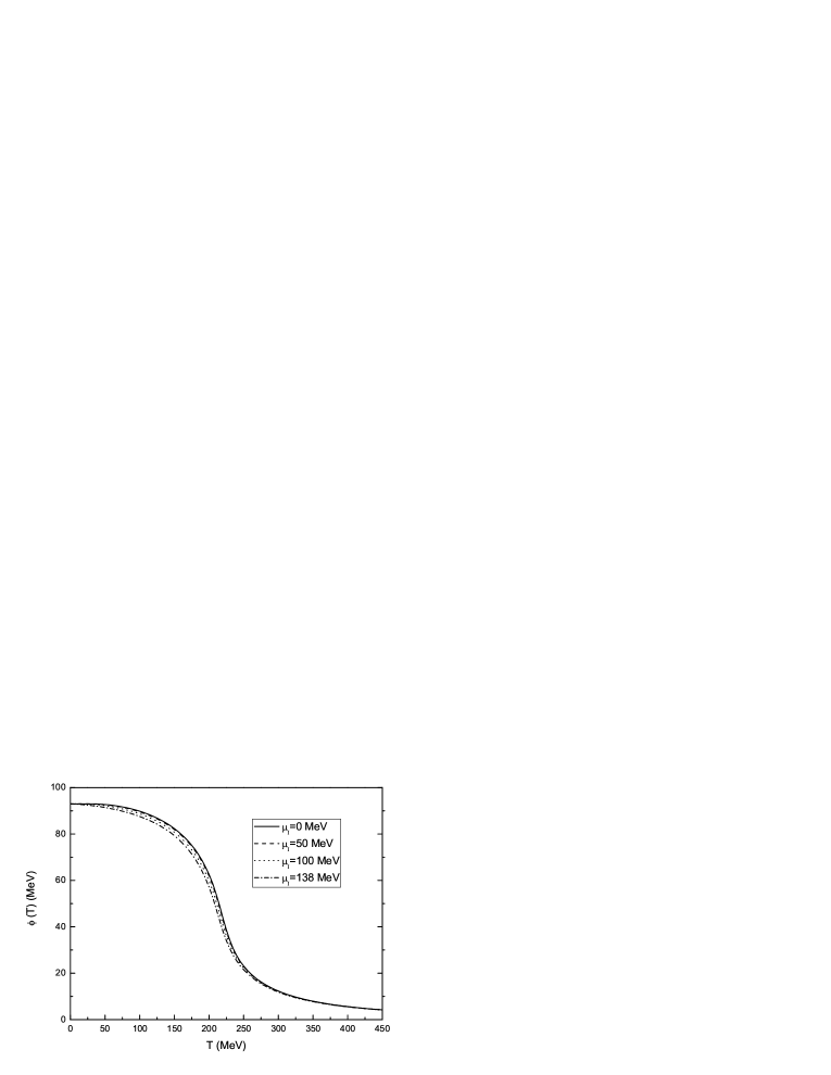
Figure 6: Evolution of the order parameter $\phi$ as a function of $T$ corresponding to $\mu_{I}=0\mathrm{MeV}$, $\mu_{I}=50\mathrm{MeV}$, $\mu_{I}=100\mathrm{MeV}$ and $\mu_{I}=138\mathrm{MeV}$ respectively.

The presence of the finite isospin chemical potential $\mu_{I}$ modifies the evolution of the order parameter $\phi$. As it is shown in Fig.6, at low temperature, for a fixed temperature, the order parameter decreases considerably as the isospin chemical potential increases. But at very high temperature, the mass of sigma is very slightly changed with the increase of the isospin chemical potential $\mu_{I}$. For various $\mu_{I}$, when the temperature increases, the order parameter decreases, and vanishes smoothly at very high temperatures. In this case, the change is not a phase transition any more and we encounter a smooth crossover from a low temperature phase to a high temperature phase. We conclude that the presence of a finite isospin chemical potential when $|\mu_{I}|\leq m_{\pi}$ does not change the nature of the chiral phase transition, only modifies the effective masses of mesons in the linear sigma model, in accordance with earlier studies Roder:2003uz Lenaghan:1999si .

V Conclusions

In summary, we have discussed the effect of the finite isospin chemical potential to the effective masses of the measons at finite temperature in the framework of the $O(4)$ linear sigma model with explicit chiral symmetry breaking. We have provided an alternative mechanism to include the isospin chemical potential in the linear sigma model. In order to get some insight into how the the isospin chemical potential could affect the chiral phase transition, we have solved the system of gap euqations numerically and found the evolution with temperature of the effective thermal masses of mesons at various $\mu_{I}$.

For neutral pions, the results for different values of finite isospin chemical potential are nearly identical to each other due to the fact that the neutral pions do not contribute to the finite isospin chemical potential $\mu_{I}$. But for charged pions, the situation is very different. At low temperature, the effective masses of charge pions are very different than that of neutral pions due to the effects of the finite isospin chemical potential, it appears that they increase more dramatically than that of neutral pions as the temperature increasing. But for high temperature, the situation has been changed, the effective mass of charged pions are similar to that of neutral pions. On the contray, the results for sigma particle are very difference from the poins. For a fixed temperature, when $T<235\mathrm{MeV}$, the mass of sigma decreases considerably with the increasing $\mu_{I}$, while for $T>235\mathrm{MeV}$, the mass of sigma increases very slightly as $\mu_{I}$ increases as well. The evolution of the order parameter $\phi$ for different $\mu_{I}$ shows the effects of the finite isospin chemical potential do not change the nature of chiral phase transition, but just modify the effective masses of mesons in the linear sigma model.

Of course, as we have already pointed out, we have not considered the pion condensate Son:2000xc ; Loewe:2002tw ; Loewe:2004mu or the pion superfluidityHe:2005nk . Our discussions for are restricted the values of $\mu_{I}\leq 138\mathrm{MeV}$. Since there will be more complicated and richer vacuum structures when $\mu_{I}$ is larger than $138\mathrm{MeV}$, it is of interest to extend our work to finite temperature for $\mu_{I}>138\mathrm{MeV}$ and discuss the pion condensate and pion superfluidity. According to the work of Shu and Li, our work can be used to study the Bose-Einstein condensation and chiral phase transition with explicit chiral symmetry breaking. All these works are in progress.

- (1) U. W. Heinz, AIP Conf. Proc. 739, 163 (2005).
- (2) D. H. Rischke, Prog. Part. Nucl. Phys. 52, 197 (2004).
- (3) M. Gell-Mann and M. Levy, Nuovo Cim. 16, 705 (1960).
- (4) K. Rajagopal and F. Wilczek, Nucl. Phys. B 399, 395 (1993).
- (5) K. Rajagopal and F. Wilczek, Nucl. Phys. B 404, 577 (1993).
- (6) E. A. Kuraev and Z. K. Silagadze, Acta Phys. Polon. B 34, 4019 (2003).
- (7) N. Petropoulos, J. Phys. G 25, 2225 (1999).
- (8) J. T. Lenaghan, D. H. Rischke and J. Schaffner-Bielich, Phys. Rev. D 62, 085008 (2000).
- (9) D. Roder, J. Ruppert and D. H. Rischke, Phys. Rev. D 68, 016003 (2003).
- (10) N. Petropoulos, arXiv:hep-ph/0402136 and reference therein.
- (11) G. Amelino-Camelia and S. Y. Pi, Phys. Rev. D 47, 2356 (1993).
- (12) G. Amelino-Camelia, Phys. Lett. B 407, 268 (1997).
- (13) J. T. Lenaghan and D. H. Rischke, J. Phys. G 26, 431 (2000).
- (14) Y. Nemoto, K. Naito and M. Oka, Eur. Phys. J. A 9, 245 (2000).
- (15) S. Shu and J. R. Li, J. Phys. G 31, 459 (2005).
- (16) D. T. Son and M. A. Stephanov, Phys. Rev. Lett. 86, 592 (2001).
- (17) J. B. Kogut, M. A. Stephanov and D. Toublan, Phys. Lett. B 464, 183 (1999).
- (18) J. B. Kogut, M. A. Stephanov, D. Toublan, J. J. M. Verbaarschot and A. Zhitnitsky, Nucl. Phys. B 582, 477 (2000).
- (19) C. Itzykson and J. B. Zuber, Quantum Field Theory (McGraw-Hill, New York, 1980)
- (20) J.F. Donoghue, E. Golowich and B. Holstein, Dynamics of the Standard Model, (Cambridge University Press, 1992).
- (21) A. Barducci, R. Casalbuoni, G. Pettini and L. Ravagli, Phys. Rev. D 69, 096004 (2004).
- (22) L. Dolan and R. Jackiw, Phys. Rev. D 9, 3320 (1974).
- (23) J. Kapusta, Finite Temperature Field Theory, Cambridge University Press, Cambridge, (1989).
- (24) M. LeBellac, Thermal Field Theory, Cambridge University Press, Cambridge, (1996).
- (25) A. Das, Finite temperature field theory, Singapore, Singapore: World Scientific (1997).
- (26) M. Loewe and C. Villavicencio, Phys. Rev. D 67, 074034 (2003).
- (27) M. Loewe and C. Villavicencio, Phys. Rev. D 70, 074005 (2004).
- (28) L. Y. He, M. Jin and P. F. Zhuang, Phys. Rev. D 71, 116001 (2005).