MCTP-06-14

Holomorphic selection rules,
the origin of the $\mu$ term, and thermal inflation

David E. Morrissey and James D. Wells
Michigan Center for Theoretical Physics (MCTP)
Physics Department, University of Michigan, Ann Arbor, MI 48109

When an abelian gauge theory with integer charges is spontaneously broken by the expectation value of a charge $Q$ field, there remains a $Z_{Q}$ discrete symmetry. In a supersymmetric theory, holomorphy adds additional constraints on the operators that can appear in the effective superpotential. As a result, operators with the same mass dimension but opposite sign charges can have very different coupling strengths. In the present work we characterize the operator hierarchies in the effective theory due to holomorphy, and show that there exist simple relationships between the size of an operator and its mass dimension and charge. Using such holomorphy-induced operator hierarchies, we construct a simple model with a naturally small supersymmetric $\mu$ term. This model also provides a concrete realization of late-time thermal inflation, which has the ability to solve the gravitino and moduli problems of weak-scale supersymmetry.

1 Introduction

Consider an Abelian gauge theory with many scalar fields $\{\phi_{i}\}$ all having integer charges $\{Q_{i}\}$, and suppose one scalar $\phi_{V}$ with charge $Q_{V}$ obtains a vacuum expectation value (VEV). It is well-known that the low-energy effective theory well below the VEV has a $Z_{Q_{V}}$ discrete symmetry [1, 2]. Fields can be assigned charges under the $Z_{Q_{V}}$ symmetry, and the effective lagrangian is built up from all operators that are $Z_{Q_{V}}$-invariant combinations of the fields.

In non-supersymmetric field theories any combination of $\{\phi_{i}\}$ and $\{\phi_{i}^{\dagger}\}$ is allowed to make gauge-invariant operators. Therefore, $Z_{Q_{V}}$ is an appropriate label for the discrete gauge symmetry of the effective theory, since it implies no distinction between allowed operators that have charge $-nQ_{V}$ under the original $U(1)$ versus those that have charge $+nQ_{V}$ (where $n$ is positive integer). There may, however, exist a hierarchy between operators of the same dimension but different absolute values of their charges [3].

In a supersymmetric field theory, merely stating that $U(1)\to Z_{Q_{V}}$ when $\phi_{V}$ develops a VEV loses information. Holomorphy of the superpotential implies that factors of $\langle\phi_{V}^{\dagger}\rangle$ alone cannot give rise directly to low-energy operators in the effective superpotential. As a result, the coefficients of two chiral operators in the low energy theory with the same mass dimension but opposite sign charges can be very different [4].

The purpose of this work is to describe the coefficient strengths of allowed operators in the effective superpotential as a function of their $U(1)$ charges in the full theory. This is the subject of Section 2. In Section 3 we apply our results to construct a small value for the $\mu$ term in the MSSM. In Section 4, we show how this mechanism for the $\mu$ term naturally gives rise to a brief period of late-time thermal inflation, which can help to dilute overabundant or late-decaying relics such as gravitinos or moduli. Our conclusions are given in Section 5. Some technical details are deferred to an Appendix.

2 Holomorphy and discrete gauge symmetries

Suppose a $U(1)$ gauge symmetry is spontaneously broken in an $\mathcal{N}=1$ supersymmetric gauge theory due to the condensation of one of more charged scalar fields. Even though the gauge symmetry is broken, the resulting effective theory will retain an invariance under spurious $U(1)$ transformations where the VEVs transform as well. The non-spurious residual discrete symmetry present in the effective theory is the subgroup of the spurious $U(1)$ that leaves the VEVs invariant. We shall make use of this spurious symmetry in discussing the additional selection rules for superpotential operators due to holomorphy. To begin, we discuss the case of a single VEV. Afterwards, we generalize to the more complicated case of two or more VEVs.

2.1 One VEV: supersymmetric $Z^{\rm hol}_{Q_{V}}$ discrete symmetry

A supersymmetric field theory can remain supersymmetric upon the condensation of a single charged field $\phi_{V}$ if there is a Fayet-Iliopoulos (FI) term in the $D$-term potential with sign opposite to that of $Q_{V}$:

$$D=Q_{V}|\phi_{V}|^{2}-\xi+\cdots~{}~{}({\rm assuming~{}}Q_{V},\xi>0).$$ (1)

For $\langle\phi_{V}\rangle=\sqrt{\xi/Q_{V}}$, the gauge symmetry is broken but supersymmetry need not be. We assume there are no $F$-terms that would break supersymmetry for a non-zero $\langle\phi_{V}\rangle$. We call the low-scale symmetry group in this case $Z^{\rm hol}_{Q_{V}}$, and the symmetry breaking path is

$$U(1)\stackrel{{\scriptstyle\langle\phi_{V}\rangle}}{{\longrightarrow}}Z^{\rm hol}_{Q_{V}}.$$ (2)

The leading operators allowed in the effective theory superpotential arise in three ways:

1. Holomorphic insertions. $\phi_{V}\to\langle\phi_{V}\rangle$ in the superpotential of the full theory. For example,

   $$W_{full}\supseteq\frac{1}{M_{*}^{a+d-3}}\,\phi_{V}^{a}\,\mathcal{O}^{(d)}({\phi_{i}})\longrightarrow\frac{\langle\phi_{V}\rangle^{a}}{M_{*}^{a}}\frac{1}{M_{*}^{d-3}}\,\mathcal{O}^{(d)}({\phi_{i}})\subseteq W_{eff},$$ (3)

   where $\mathcal{O}^{(d)}({\phi_{i}})$ is an operator of mass dimension $d$ composed of light fields $\{\phi_{i}\}$, and $M_{*}$ denotes the ultraviolet cutoff of the theory. This mechanism generates insertions of $\langle\phi_{V}\rangle/M_{*}$ (but not $\langle\phi^{\dagger}_{V}\rangle/M_{*}$), and therefore only operators $\mathcal{O}^{(d)}({\phi_{i}})$ with total charge equal to $0,-Q_{V},-2Q_{V},\ldots$ in the full theory can be generated in this way.

2. Inverse-holomorphic insertions. These arise from integrating out heavy fields whose masses derive from $\langle\phi_{V}\rangle$. Mass terms for the superfields in the original superpotential are analytic in the VEVs leading to new operators suppressed by $1/\langle\phi_{V}\rangle$ when these massive fields are integrated out. As an example, consider a theory with the superpotential

   $$W=\lambda_{1}\,\phi_{4}\,\phi_{-2}^{2}+\lambda_{2}\,\phi_{-2}\,\phi_{1}^{2},$$ (4)

   where the field $\phi_{q}$ has charge $q$. If $\phi_{4}$ obtains a VEV, $\phi_{-2}$ gets a large mass $\sim\langle\phi_{4}\rangle$. Upon integrating these fields out, the leading term in the effective superpotential is

   $$W_{eff}\supseteq-\frac{\lambda_{2}^{2}}{4\lambda_{1}\langle\phi_{4}\rangle}\,\phi_{1}^{4}.$$ (5)

   This mechanism produces operators with insertions of $1/\langle\phi_{V}\rangle$ of the form

   $$W_{eff}\supseteq\frac{M_{*}^{a}}{\langle\phi_{V}\rangle^{a}}\,\frac{1}{M_{*}^{d-3}}\,\mathcal{O}^{(d)}(\phi_{i}).$$ (6)

   The possible charges of the operators $\mathcal{O}^{(d)}(\phi_{i})$ are $+Q_{V},+2Q_{V},\ldots$.

3. Supersymmetry breaking insertions. Supersymmetry breaking terms can transfer Kähler potential terms to the effective superpotential. This last mechanism can be schematically represented by

   $$\int d^{4}\theta\;\frac{X^{\dagger}}{M_{*}}\,\frac{1}{M_{*}^{a+b+d-2}}\,\phi_{V}^{a}\phantom{\!\!(}{\phi_{V}^{\dagger}}\phantom{)\!\!\!}^{b}\,\mathcal{O}^{(d)}\longrightarrow\int d^{2}\theta\;\frac{F_{X}^{\dagger}}{M_{*}^{2}}\,\frac{\langle\phi_{V}\rangle^{a}\langle\phi_{V}^{\dagger}\rangle^{b}}{M_{*}^{a+b}}\,\frac{1}{M_{*}^{d-3}}\,\mathcal{O}^{(d)}$$ (7)

   This mechanism always involves the supersymmetry breaking scale through the combination $\tilde{m}=F_{X}/M_{*}$, as well as possible insertions of both $\langle\phi_{V}\rangle/M_{*}$ and $\langle\phi_{V}^{\dagger}\rangle/M_{*}$.

As expected, at the level of supersymmetry breaking, all operators consistent with the full $Z_{Q_{V}}$ symmetry are allowed. However, in the supersymmetric limit ($\tilde{m}\to 0$) operators with total charge equal to $-n\,Q_{V}$, where $n$ is a positive integer, are generated by holomorphic insertions of $\langle\phi_{V}\rangle$ (mechanism 1), while operators with total charge $+n\,Q_{V}$ arise from integrating out holomorphic fields leading to inverse-holomorphic insertions of $1/\langle\phi_{V}\rangle$ (mechanism 2). The coefficients of two operators with the same dimension but opposite charge can therefore be very different. If $\langle\phi_{V}\rangle\ll M_{*}$, operators generated by mechanism 2 are potentially much larger than those from mechanism 1. This is the essential difference between $Z_{Q_{V}}$ and $Z_{Q_{V}}^{hol}$.

The distinction between $Z_{Q_{V}}$ and $Z^{\rm hol}_{Q_{V}}$ remains significant if there is a hierarchy $\tilde{m}\ll\left<\phi_{V}\right>$. In this case the operators containing insertions of $\tilde{m}$ are typically extremely suppressed relative to those generated by mechanisms 1 and 2 above. There is, however, one important exception. The operators generated by mechanism 2 depend on which fields in the full theory get large masses due to the VEV. If a particular operator with charge $+nQ_{V}$ does not arise in the effective superpotential due to mechanism 2, the operator will only appear due to mechanism 3. On the other hand, if the superpotential of the full theory is completely generic, mechanism 1 will generate every possible operator with charge $-nQ_{V}$ consistent with the other symmetries of the theory.

2.2 Several VEVs: flat directions

The $D$-term potential of a supersymmetric abelian gauge theory is

$$V_{D}=\frac{g^{2}}{2}D^{2},~{}~{}{\rm where}~{}~{}D=\sum_{i}Q_{i}|\phi_{i}|^{2}+\xi.$$ (8)

For simplicity we assume $\xi=0$, although our generic results do not depend on this choice. An anomaly-free theory must have charges of either sign. Thus, whether or not $\xi$ is present, there is always a supersymmetric minimum of $V_{D}$ in which two fields with opposite-sign charges develop VEVs.

We shall focus on the case of two fields $\phi_{a}$ and $\phi_{-b}$ with charges $a$ and $-b$ obtaining large VEVs. In practice, this can occur if some fields have tachyonic soft mass squareds. The $D$-term potential cancels provided their expectation values satisfy

$$b|\langle\phi_{a}\rangle|^{2}=a|\langle\phi_{-b}\rangle|^{2}.$$ (9)

Since the $D$-term potential is completely flat along this direction, no particular value of $\langle\phi_{a}\rangle$ is favored. This degeneracy is lifted and the VEVs are fixed by superpotential and supersymmetry breaking operators. If the superpotential operators are small, either because they are higher dimensional or if they have tiny couplings, the potential remains almost flat along this direction, and the field VEV can be very large compared to the scale of supersymmetry breaking.

The $U(1)$ symmetry is broken along the almost flat direction by the VEVs of $\phi_{a}$ and $\phi_{-b}$. The residual symmetry is $Z_{(a,-b)}$ where $(a,-b)$ is the greatest common divisor of $a$ and $b$. If $a$ and $b$ are relatively prime numbers, there is no residual symmetry at all. Even so, in a supersymmetric theory there is additional information to be had. To emphasize this point, we indicate the symmetry breaking pattern as

$$U(1)\stackrel{{\scriptstyle\langle\phi_{a}\rangle,\langle\phi_{-b}\rangle}}{{\longrightarrow}}Z^{\rm hol}_{(a,-b)}~{}~{}({\rm supersymmetric}).$$ (10)

The distinguishing feature between $Z^{\rm hol}_{(a,-b)}$ and $Z_{(a,-b)}$ are the relative sizes of operators appearing in the effective theory.

To describe the effective theory below the $U(1)$ breaking scale, it is helpful to write $\phi_{a}$ and $\phi_{-b}$ in the form [5]

$$\phi_{a}=\sqrt{{b}}\,\tau\,e^{-ia\Omega},~{}~{}~{}~{}~{}\phi_{-b}=\sqrt{{a}}\,\tau\,e^{ib\Omega},$$ (11)

where $\tau$ and $\Omega$ are chiral superfields. The phase $\Omega$ can be gauged away completely, in which case the superfield degree of freedom is transferred to the $U(1)$ gauge multiplet which is integrated out. The degrees of freedom associated with $\tau$ describe excitations along the flat direction. To see why, note that all $D$-flat directions of condensing fields can be parametrized by the gauge invariant chiral polynomials of these fields [6, 7]. In the present case, the only possibility is

$$T=\phi_{a}^{b}\phi^{a}_{-b}=\sqrt{{a^{b}b^{a}}}\,\tau^{a+b},$$ (12)

which is clearly in one-to-one correspondence with $\tau$.

The operators in the low-energy superpotential are formed much like in the case of a single VEV. Instead of replacing $\phi_{a}$ and $\phi_{-b}$ with their expectation values, however, they are replaced by their expressions from Eq. (11) with $\Omega\to 0$. The excitations of $\tau$ around its expectation value are light, and are thus still present in the effective theory. Integrating out heavy fields whose masses are proportional to the VEVs will also generate operators with powers of $\phi_{a}$ and $\phi_{-b}$ in denominators. The possible superpotential operators are therefore

$$\frac{\phi_{a}^{s}\phi_{-b}^{t}}{M_{*}^{d+s+t-3}}\;\mathcal{O}^{(d,Q)},~{}~{}~{}~{}~{}~{}~{}Q=-sa+tb,$$ (13)

where $\mathcal{O}^{(d,Q)}$ refers to an operator of dimension $d$ and charge $Q$, $s$ and $t$ are (possibly negative) integers, and $\phi_{a}$ and $\phi_{-b}$ are to be expressed in terms of $\tau$. In addition to these operators there are contributions from supersymmetry breaking, but they are generally subleading. The operator hierarchies due to $Z^{\rm hol}_{(a,-b)}$ are best understood through an illustration. Below, we derive a model of the $\mu$ term based on these considerations.

3 A small supersymmetric $\mu$ term

The operator hierarchy implied by a $Z^{\rm hol}_{(a,-b)}$ symmetry together with an almost flat direction provides a mechanism for generating a naturally weak-scale value of the supersymmetric $\mu$-term. Let $a$ and $b$ be relatively prime integers, and suppose the expectation values of the fields $\phi_{a}$ and $\phi_{-b}$ break a $U(1)_{x}$ gauge symmetry under which the $H_{u}\!\cdot\!H_{d}$ superfield bilinear has charge $+1$. The dominant superpotential terms in the full theory are

$$W_{full}=\lambda_{1}\,\left(\frac{\phi_{a}^{q_{a}}\phi_{-b}^{q_{b}}}{M_{*}^{q_{a}+q_{b}-1}}\right)\,H_{u}\!\cdot\!H_{d}+\lambda_{2}\,\left(\frac{\phi_{a}^{b}\phi_{-b}^{a}}{M_{*}^{a+b-3}}\right),$$ (14)

where $M_{*}\sim M_{GUT}$ or $M_{\rm Pl}$ is an ultraviolet cutoff scale, and $q_{a}$ and $q_{b}$ are the smallest positive integers such that $q_{a}a-q_{b}b=-1$. These superpotential operators break $D$-flatness and drive the VEVs to zero. To ensure non-zero expectation values, we include tachyonic soft masses

$$\mathscr{L}_{soft}=m_{a}^{2}|\phi_{a}|^{2}+m_{b}^{2}|\phi_{-b}|^{2}.$$ (15)

Since the stabilizing effects of $F$-terms in the potential are suppressed by powers of $M_{*}$, the vacuum expectation values of $\phi_{a}$ and $\phi_{-b}$ are much larger than the soft masses. A similar structure of the full potential for a $\mu$-term solution can be found in Ref. [8].

Writing $\phi_{a}$ and $\phi_{-b}$ in terms of $\tau$, the leading terms in the scalar potential for $\tau$ are

$$V_{\tau}=-\tilde{m}^{2}|\tau|^{2}+\tilde{\lambda}_{2}M_{*}^{4}\left(\frac{|\tau|}{M_{*}}\right)^{2(a+b)-2}$$ (16)

where $\tilde{m}^{2}$ and $\tilde{\lambda}_{2}$ are obtained straightforwardly from the full potential. The scalar potential is minimized when

$$\langle|\tau|\rangle\sim M_{*}\left(\frac{\tilde{m}}{M_{*}}\right)^{1/(a+b-2)}.$$ (17)

So far, the potential depends only on the modulus of $\tau$. A parametrically important contribution to the potential that fixes the phase of $\tau$ is the supersymmetry breaking operator

$$\int d^{2}\theta\;\frac{X}{M_{*}}\,\frac{\phi_{a}^{b}\phi_{-b}^{a}}{M_{*}^{a+b}}\,M_{*}^{3}\longrightarrow\tilde{m}M_{*}^{3}\left(\frac{\tau}{M_{*}}\right)^{a+b}.$$ (18)

The solution for $\langle\tau\rangle$ implies an effective $\mu$ term of size

$$\mu_{eff}\sim M_{*}\left(\frac{\tilde{m}}{M_{*}}\right)^{\frac{q_{a}+q_{b}}{a+b-2}}.$$ (19)

Clearly, not all choices of $a$ and $b$ will work since $(q_{a}+q_{b})/(a+b-2)=1$ is needed to get $\mu_{eff}\sim\tilde{m}$. A general solution that guarantees this relation for any values of $\tilde{m}\ll M_{*}$ is

$$(a,-b)=(n+1,-n)~{}~{}~{}{\rm implying}~{}~{}~{}q_{a}=n-1,~{}q_{b}=n~{}~{}\Rightarrow\frac{q_{a}+q_{b}}{a+b-2}=1,$$ (20)

where $n$ is a positive integer.

We note that different choices of $(a,-b)$ can obtain different hierarchies of the $\mu$ term with respect to the supersymmetry breaking scale $\tilde{m}$. This could be of importance for model-building in split supersymmetry [9], when the $\mu$ term is desired to be much smaller than $\tilde{m}$ in order for gauge coupling unification to work out. For example, choosing parameters such that the exponent in Eq. (19) is greater than 1 gives

$$\frac{q_{a}+q_{b}}{a+b-2}=1+\Delta,~{}~{}\Rightarrow\mu_{eff}=\tilde{m}\left(\frac{\tilde{m}}{M_{*}}\right)^{\Delta}.$$ (21)

The value of $\Delta$ can then be tuned, from the model-building perspective, to suppress the $\mu$ term compared to the typical superpartner mass of $\tilde{m}$.

In passing to the effective theory, we must verify that corrections involving inverse powers of $\phi_{a}$ and $\phi_{-b}$ do not generate a $\mu_{eff}$ larger than the one we have found. For the charges $a=n+1$ and $b=n$, the only dangerous gauge-invariant combination is

$$\frac{1}{\phi_{n+1}\phi_{-n}}\,H_{u}\!\cdot\!H_{d}.$$ (22)

For this to be an operator in the superpotential, three powers of $M_{*}$ or $\tilde{m}$ are needed to make up the dimension. Since positive powers of $M_{*}$ cannot arise from integrating out at scale $|\tau|\lesssim M_{*}$, there are no large corrections to $\mu_{eff}$. Similarly, any contribution from supersymmetry breaking must come in with a power of $\tilde{m}$, and is therefore sub-leading as well. Thus, we see that the strong correlation between the charge and dimension of superpotential operators allowed by $Z^{\rm hol}_{(a,-b)}$ leads to a naturally small effective $\mu$ term.

As it stands, the model is potentially anomalous with respect to the new $U(1)_{x}$ gauge symmetry. To avoid anomalies, new exotic matter is typically required and this can disrupt gauge unification. Let us assume that the $U(1)_{x}$ charges of the MSSM fields are family universal, and are consistent with an embedding in $SU(5)$: $q=u=e$ and $d=l$. For the usual MSSM superpotential operators to be gauge invariant, with $(h_{u}+h_{d})=1$, we must have

$$q=-\frac{1}{2}h_{u},~{}~{}~{}~{}~{}~{}~{}l=\frac{3}{2}h_{u}-1,$$ (23)

Suppose we add to the model two pairs of doublets,

$$D_{1}\oplus\overline{D}_{1}=({\bf 1},{\bf 2},\frac{1}{2})_{q_{1}}\oplus({\bf 1},{\bf 2},-\frac{1}{2})_{\bar{q}_{1}},~{}~{}~{}~{}~{}D_{2}\oplus\overline{D}_{2}=({\bf 1},{\bf 2},\frac{1}{2})_{q_{2}}\oplus({\bf 1},{\bf 2},-\frac{1}{2})_{\bar{q}_{2}},$$ (24)

with $U(1)_{x}$ charges such that $q_{1}+\bar{q_{1}}=-(n+1)$ and $q_{2}+\bar{q}_{2}=n$. Since the doublets are vector-like under the SM gauge group, they will not induce any pure SM anomalies. The quantum numbers of these doublets also imply that the mixed $SU(3)_{c}^{2}U(1)_{x}$, $SU(2)_{L}^{2}U(1)_{x}$, and $U(1)_{Y}^{2}U(1)_{x}$ anomaly conditions all have the form

$$X_{i}-n_{g}=0,~{}~{}~{}~{}~{}i=1,2,3$$ (25)

where the $X_{i}$ represent the contributions from SM exotics other than $D_{1}$, $\overline{D}_{1}$, $D_{2}$, and $\overline{D}_{2}$. All three anomaly conditions can be satisfied by including complete vector-like (with respect to the SM) $SU(5)$ multiplets, each of which automatically generates $X_{1}=X_{2}=X_{3}$ in our normalization. Furthermore, such multiplets do not contribute at all to the $U(1)_{Y}U(1)_{X}^{2}$ mixed anomaly, for which the cancellation condition is

$$0=(2h_{u}-1)-(q_{1}-\bar{q}_{1})\,(n+1)+(q_{2}-\bar{q}_{2})\,n.$$ (26)

One possible solution is $q_{1}=\bar{q}_{1}$, $q_{2}=\bar{q}_{2}$, and $h_{u}=1/2$. Thus, by adding two pairs of doublets and some number of complete $SU(5)$ multiplets, it is possible to cancel all the SM-$U(1)_{x}$ mixed anomalies in the model. The remaining $U(1)_{x}^{3}$ and gravity-$U(1)_{x}$ anomalies can be eliminated by including SM gauge singlets (see, e.g., [10, 11]).

Our solution to the anomaly constraints can also be consistent with gauge unification. In this regard, only the two pairs of doublets pose a threat. However, given their charges they can obtain large masses when $\phi_{n+1}$ and $\phi_{-n}$ condense from the superpotential operators

$$W\supset\phi_{n+1}\bar{D}_{1}D_{1}+\phi_{-n}\bar{D}_{2}D_{2}.$$ (27)

For very large VEVs, within a couple of orders magnitude of $10^{16}$ GeV, the doublets will be very heavy, they will only slightly disrupt the running of the gauge couplings, and unification will be preserved. This mechanism is attractive because it circumvents some of the difficulties associated with more common $U(1)_{x}$ solutions to the $\mu$ problem with respect to unification [11].

4 Thermal inflation

The extremely shallow potentials that arise naturally from breaking a supersymmetric $U(1)$ gauge symmetry can also play an important role in the early universe. When a potential is almost flat, thermal corrections often induce a metastable false vacuum. For a system stuck in such a vacuum, the excess vacuum energy may come to dominate the energy density of the universe giving rise to a period of late-time thermal inflation [12, 13]. In the present section we show how this scenario is realized within the model considered above.

The effect of thermal corrections on the potential depends on the temperature relative to the zero-temperature expectation value, $\tau_{0}\equiv\langle\tau\rangle_{T=0}$ [14]. At very high temperature, $T\gg\tau_{0}$, the exotic $U(1)_{x}$ gauge bosons and gauginos are abundant in the plasma, and they induce positive soft squared masses for $\phi_{a}$ and $\phi_{-b}$ of order $g_{x}^{2}T^{2}\gg\tilde{m}^{2}$. In this case, the unique minimum of the finite-temperature effective potential lies at the origin, where the $U(1)_{x}$ gauge symmetry is unbroken.

At temperatures smaller than $\tau_{0}$, but still much larger than $\tilde{m}$, the potential has two minima [14]. For small field values, $|\tau|\ll\tau_{0}$, the gauge bosons are light and they again generate soft squared masses of order $g_{x}^{2}T^{2}$. These thermal corrections induce a local minimum at the origin. Conversely, for large field values, $|\tau|\gg T$, the gauge bosons and gauginos are very heavy and the thermal corrections they induce are therefore Boltzmann-suppressed. Since the couplings of the $\tau$ excitations to other fields are suppressed by powers of $\tau/M_{*}$, the effective potential is only slightly modified for these large values of $|\tau|$, and a minimum near $|\tau|=\tau_{0}$ persists. For $T\ll\tau_{0}$, this is the global minimum of the potential. The potential is illustrated in Fig. 1.

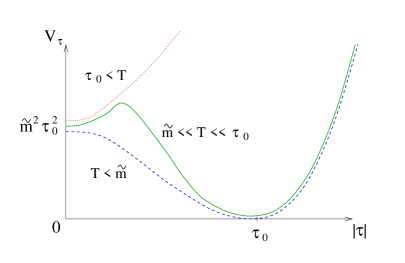
Figure 1: An illustration of the temperature-corrected scalar potential. The red (dotted) line shows the potential at very high temperatures $T\gg\tau_{0}$, while the green (solid) line corresponds to intermediate temperatures in the range $\tilde{m}\ll T\ll\tau_{0}$, and the lower blue (dashed) line shows the potential for $T\ll\tilde{m}$.

The cosmological effects of this potential are determined by whether or not $\tau$ is trapped in the local vacuum at $\tau=0$ after primordial inflation. This will almost certainly be the case if the reheating temperature after inflation exceeds $\tau_{0}$. Even for reheating temperatures below $\tau_{0}$, the $\tau$ field may be trapped at the origin by the “Hubble mass” operator, $H^{2}|\tau|^{2}$, provided it is generated with a positive sign [15]. If the field is not trapped at the origin, it will behave as a moduli field, and will be cosmologically dangerous if it decays after the onset of nucleosynthesis.

Let us assume that the $\tau$ field becomes trapped at the origin. The tunneling rate from this local minimum to the true vacuum is typically extremely small for $T>\tilde{m}$ [16], so this minimum is metastable until $T\sim\tilde{m}$. The vacuum energy of the false vacuum is of order $\tilde{m}^{2}\tau_{0}^{2}$ compared to the value at the global minimum. If the universe is initially radiation-dominated, then as the temperature cools below $T\sim\sqrt{\tilde{m}\tau_{0}}$ the excess vacuum energy becomes the dominant component of the total energy density, and the universe begins to inflate. The Hubble rate during this era is

$$H=H_{0}=\sqrt{\frac{8\pi}{3}}\frac{\tilde{m}\tau_{0}}{M_{\rm Pl}},$$ (28)

which determines the expansion rate, $a(t)=a(t_{0})e^{H_{0}(t-t_{0})}$. The exponential expansion ceases when the temperature falls below $T\sim\tilde{m}$ yielding a total number of $e$-foldings

$$N_{e}\simeq\ln\left(\frac{\sqrt{\tilde{m}\tau_{0}}}{\tilde{m}}\right)=\frac{1}{2}\ln\left(\frac{\tau_{0}}{\tilde{m}}\right).$$ (29)

This number is of order $10$ for $\tilde{m}\sim 10^{3}$ GeV and $\tau_{0}\sim 10^{12}$ GeV. Such a small number of $e$-foldings is not enough to disrupt the density perturbation induced by primordial inflation [17]. The amount of inflation will be somewhat less if the universe is matter dominated before thermal inflation. For example, a moduli field with a Planck scale VEV and a shallow potential with curvature of order $\tilde{m}$ will dominate the energy density of the universe once the temperature falls below $T\sim\sqrt{\tilde{m}M_{\rm Pl}}$. This postpones the start of thermal inflation, reducing the temperature at which inflation begins by a factor of $(\tau_{0}/M_{\rm Pl})^{1/6}$ [12], and decreasing the number of $e$-foldings by an amount $\ln(\tau_{0}/M_{\rm Pl})/6$.

Once $T$ falls below $\tilde{m}$, the $\tau$ field rolls down the potential towards the global minimum and begins to oscillate. The oscillations dominate the total energy density until the $\tau$ field decays away. Assuming the coupling between $\tau$ and the Higgs fields to be of the form of Eq. (14), we estimate this decay rate to be

$$\Gamma_{\tau}=\gamma\frac{\tilde{m}^{3}}{\tau_{0}^{2}},$$ (30)

where $\gamma$ is a dimensionless constant less than or on the order of unity. If the products of this decay thermalize rapidly, the reheating temperature after the decay is [18]

$$T_{RH} \simeq \left(\frac{3}{\pi^{3}g_{*}}\right)^{1/4}(M_{\rm Pl}\,\Gamma_{\tau})^{1/2}$$

$$\simeq 3~{}\mbox{GeV}\;\left(\frac{10}{g_{*}}\right)^{1/4}\left(\frac{\tilde{m}}{1\mbox{TeV}}\right)^{3/2}\left(\frac{10^{13}\mbox{GeV}}{\tau_{0}}\right)\,\gamma^{1/2}.$$

The reheating temperature must be greater than about $5$ MeV to preserve the successful predictions of nucleosynthesis [19], and this implies an upper bound on $\tau_{0}$ on the order of $10^{16}$ GeV (for $\gamma=1$ and $\tilde{m}=1$ TeV). For comparison, if we set $M_{*}=M_{\rm Pl}/\sqrt{8\pi}$ in Eq. (17), we find $\tau_{0}\lower 3.01385pt\hbox{$\;\stackrel{{\scriptstyle\textstyle<}}{{\sim}}\;$}2\times 10^{13},~{}2\times 10^{15},~{}5\times 10^{16}$ GeV for $(a+b)=5,~{}7,~{}9$ where $a$ and $b$ are the powers in Eq. (14).

Thermal inflation provides a mechanism to reduce the density of unwanted relics. In addition to dilution by the inflationary expansion, a decoupled relic is diluted even further by the entropy released when the $\tau$’s decay by a factor of order $\sqrt{\tilde{m}^{5}M_{\rm Pl}/\tau_{0}^{6}}$. This dilution factor may even be needed to reduce the relic abundance of late-decaying gravitinos and moduli that could disrupt big bang nucleosynthesis, or of other particles with an overly large energy density at late times [20]. For gravitinos and moduli, the dilution factor in our model is sufficient to lower their abundance to an acceptable level provided $\tau_{0}\gtrsim 10^{10}$ GeV [12]. Unfortunately, desirable relics such as a dark matter particle or a baryon asymmetry will also be diluted. The extent to which they are regenerated depends on $T_{RH}$, as well as the details of the $\tau$ decay. Even for very low reheating temperatures, well below 1 GeV, dark matter LSP’s can be created non-thermally in the decays of the $\tau$ [21], leading to a nonthermal dark matter candidate. The baryon asymmetry is more difficult to explain within this scenario, but it might be generated through new dynamics associated with the flat direction [22, 23].

5 Conclusions

We have examined the operator hierarchies that emerge from the spontaneous breakdown of a $U(1)$ gauge symmetry in a supersymmetric theory. The constraints induced by holomorphy lead to large hierarchies between operators with the same mass dimension but different charges. We have made use of these hierarchies to construct a naturally small supersymmetric $\mu$ term, as well as a simple realization of thermal inflation. The solution to the $\mu$ term presented here lacks some of the challenges of the more common approach of employing the vacuum expectation value of a singlet field $S$ in the superpotential $\lambda SH_{u}\!\cdot\!H_{d}$ to form $\mu_{eff}=\lambda\langle S\rangle$ [11]. Furthermore, the cosmology of thermal inflation, which is a natural byproduct of the $Z_{(a,-b)}^{hol}$ solution to the $\mu$ term presented in this work, allows for large suppressions of unwanted relics, such as late-decaying gravitino and moduli fields, while simultaneously allowing for the existence of a good cold dark matter candidate.

Appendix: Integrating out heavy superfields

In this appendix we describe the process of integrating out fields that become heavy upon the spontaneous breaking of a $U(1)$ gauge symmetry. Along the way, we provide evidence for our claim that the operators in the resulting low-energy effective superpotential arise from the three mechanisms we described in the text: holomorphic insertions, inverse-holomorphic insertions, and supersymmetry breaking insertions. Throughout the analysis, we assume that the symmetry breaking VEVs are much larger than the scale of supersymmetry breaking, and that the superpotential is small in units of the VEV. (For example, this is the case if the superpotential contains only higher dimensional operators.) If this condition holds true, the directions in field space that would be flat in the absence of a superpotential or supersymmetry breaking remain almost flat after the inclusion of these effects.

When there are almost flat directions, it is convenient to think of the process of forming the effective theory below the symmetry breaking scale as a three-step process. The first step consists of parametrizing the $D$-flat directions, and integrating out the vector multiplet and the fields orthogonal to the flat directions at an arbitrary point well out in the moduli space. The second step is to integrate out fields that do not condense, but that develop large supersymmetric masses as a result of the symmetry breaking. Thirdly, supersymmetry breaking is included as a small perturbation. For this procedure to be self-consistent, the VEVs of the moduli fields must be much larger than the supersymmetry breaking terms.

Vector multiplets

Consider the case of two chiral superfields, $\phi_{a}$ and $\phi_{-b}$, obtaining large VEVs and a collection of other fields $\phi_{i}$ that do not. The fields $\phi_{a}$ and $\phi_{-b}$ have charges $a$ and $-b$ respectively, and break the $U(1)$ symmetry when they condense. The leading terms in the Kähler potential are

$$\int d^{4}\theta\;{K}=\int d^{4}\theta\;\left({\phi_{a}}^{\dagger}e^{a\mathscr{V}}\phi_{a}+{{\phi}_{-b}^{\dagger}}e^{-b\mathscr{V}}\phi_{-b}+{\phi}_{i}^{\dagger}e^{q_{i}\mathscr{V}}e^{\mathscr{V}_{ew}}\phi_{i}\right).$$ (32)

Here, we have allowed for the possibility that the $\phi_{i}$ also transform under another gauge group.

Now suppose $\phi_{a}$ and $\phi_{-b}$ develop large expectation values, but the $\phi_{i}$ do not. Following [5], we parametrize these fields as

$$\phi_{a} = \sqrt{b}\,e^{-ia\Omega}\,\tau$$ (33)

$$\phi_{-b} = \sqrt{a}\,e^{ib\Omega}\,\tau$$

$$\phi_{i} = e^{-iQ_{i}\Omega}\tilde{\phi}_{i},$$

where $\Omega$, $\tau$, and $\tilde{\phi}_{i}$ are chiral superfields. To maintain this parametrization under $U(1)$ supergauge transformations, we take $\Omega$ to transform by a shift, and $\tau$ and $\tilde{\phi}_{q}$ to be invariant. Note that $\Omega$ can be gauged away completely. The motivation for this form is that $\tau$ is in one-to-one correspondence with the unique gauge invariant polynomial that we can make from $\phi_{a}$ and $\phi_{-b}$,

$$\phi_{a}^{b}\phi_{-b}^{a}=\sqrt{a^{a}b^{b}}\tau^{a+b}.$$ (34)

Thus, $\tau$ parametrizes the $ab$ flat direction [7].

The vector multiplet can be integrated out using its superfield equation of motion,

$$0 = \frac{d{K}}{d\mathscr{V}}+(D^{2},\bar{D}^{2}~{}terms)$$

$$\simeq ab\,{\tau}^{\dagger}\tau\,e^{a[\mathscr{V}-i(\Omega-\bar{\Omega}^{\dagger})]}-ab\,{\tau}^{\dagger}\tau\,e^{-b[\mathscr{V}-i(\Omega-\bar{\Omega}^{\dagger})]}+Q_{i}\,{\tilde{\phi}}_{i}^{\dagger}e^{\mathscr{V}_{ew}}\tilde{\phi}_{i}\,e^{Q_{i}[\mathscr{V}-i(\Omega-{\Omega}^{\dagger})]}.$$

Treating the $\phi_{i}$ as small and $\tau$ as large, the solution is

$$\mathscr{V}-i(\Omega-{\Omega}^{\dagger})=0+\mathcal{O}\left(\frac{{\tilde{\phi}}_{i}^{\dagger}e^{\mathscr{V}_{ew}}\tilde{\phi}_{i}}{{\tau}^{\dagger}\tau}\right).$$ (36)

Therefore the leading terms in the Kähler potential of the effective theory are

$${K}_{eff}=(a+b)\,{\tau}^{\dagger}\tau+{\tilde{\phi}}_{i}^{\dagger}e^{\mathscr{V}_{ew}}\tilde{\phi}_{i}.$$ (37)

Up to a trivial rescaling and small corrections, the Kähler potential for $\tau$ is canonical.

If the full theory also has a superpotential, then by gauge invariance it can only be a function of $\tau$ and $\tilde{\phi}_{i}$, but not $\Omega$. Thus, in passing to the effective theory, the procedure of integrating out the vector multiplet (and in the process the gauge artifact $\Omega$) only affects the Kähler potential. The resulting superpotential is simply given by its expression in the full theory with the replacements $\phi_{a,-b}\to\tau$ and $\phi_{i}\to\tilde{\phi}_{i}$. This is the source of the holomorphic insertions described in the text. The light field corresponding to the almost flat direction appears in the effective theory by expanding $\tau$ about its VEV.

The case of a single field obtaining a VEV can be treated in the same way. Now there is no flat direction, and the condensing field is eaten by the vector multiplet. This is manifest if we express the condensing field $\phi_{V}$ in the form

$$\phi_{V}=e^{-iQ_{V}\,\Omega}\,\langle\phi_{V}\rangle,$$ (38)

where $\langle\phi_{V}\rangle=\xi/Q_{V}$ (see Eq. (1)), and then make a supergauge transformation to remove $\Omega$. The equation of motion for the vector multiplet then gives $\mathscr{V}=0$, up to small corrections of order $|\phi_{i}|^{2}/\langle|\phi_{V}|^{2}\rangle$. By gauge invariance, $\Omega$ cannot appear in the full superpotential, so in the effective superpotential $\phi_{V}$ is simply replaced by its expectation value. There is no expansion about this value because there is no flat direction.

When three or more fields develop large VEVs, we can again use a similar technique. However, in this case the equation of motion for $\mathscr{V}$ is typically very complicated, and the effective Kähler potential need not have the minimal form found in the two VEV scenario.

Chiral multiplets

The next step is to consider the effects of the VEVs on the superpotential. In the effective theory, the flat direction fields such as $\tau$ are expanded about their VEVs. By construction, these fields have masses parametrically smaller than the VEVs. However, the appearance of large expectation values can give rise to large supersymmetric masses for other fields that do not condense. These heavy fields should also be integrated out. We show here that the integration out procedure can be performed in such a way that the resulting effective superpotential will be holomorphic in both the light fields and the parameters in the full superpotential, up to higher derivatives and supersymmetry breaking [24].

Suppose only one chiral superfield $\Phi$ develops a large mass due to the VEVs. The full superpotential must therefore be of the form

$$W_{full}=\frac{1}{2}M\Phi^{2}-f(\Phi,\phi),$$ (39)

where $M$ denotes the large mass, proportional to the VEV, and $\phi$ refers to any field other than $\Phi$. By assumption, $f(\Phi,\phi)$ contains no positive dimensional couplings unless they are much smaller than $M$. The equation of motion for $\Phi$ can be expressed in the form

$$\Phi=\frac{1}{M}\left[\frac{\partial f(\Phi,\phi)}{\partial\Phi}+\frac{\bar{D}^{2}}{4}\frac{\partial K}{\partial\Phi}\right],$$ (40)

where $K$ denotes the Kähler potential. We can solve iteratively for $\Phi$ by replacing $\Phi$ on the right hand side with this relation. Note that each repetition of this procedure always brings in an additional power of $1/M$, and thus the solution is expected to converge rapidly. Since inverse powers of $M$ appear in the solution for $\Phi$, they will also appear in the effective superpotential. This is the source of the inverse holomorphic insertions (mechanism 2) described in the text.

We claim that to any order in this procedure, the resulting expression for $\Phi$ can be written in the form

$$\Phi=(holomorphic)+\frac{\bar{D}^{2}}{4}(maybe~{}non\!-\!holomorphic),$$ (41)

where the first term is holomorphic in both the fields and all the superpotential parameters. At lowest order in the $1/M$ expansion we set $\Phi=0$ on the right hand side of Eq. (40) and our assertion is clearly satisfied. If we assume that at the $n$-th order our claim is true, then inserting Eq. (40) and expanding, we see that $\Phi$ will have the form of Eq. (41) at the $(n+1)$-th order as well. Thus, our assertion follows by induction.

This result is enough to show that the effective superpotential will be holomorphic in the couplings of the full superpotential, up to supersymmetry breaking and higher derivative operators. Inserting the full solution for $\Phi$, in the form of Eq. (41), into the superpotential we obtain holomorphic terms without derivatives, as well as terms of the type

$$\int d^{2}\theta\;G(\phi)\left(\frac{-\bar{D}^{2}}{4}\right)H({\phi}^{\dagger}).$$ (42)

These can be converted into Kähler potential terms using the fact up to a total derivative, $-\bar{D}^{2}/4$ is equivalent $d^{2}\bar{\theta}$ [25]. Putting our solution for $\Phi$ into the Kähler potential, there can also arise terms of the form

$$\int d^{4}\theta\;A(\phi)\left(-\frac{D^{2}}{4}\right)B(\phi)=\int d^{2}\theta\;{A}(\phi)\partial^{2}{B}(\phi),$$ (43)

where we have made use of the identity $(\bar{D}^{2}D^{2}/16)\phi=\partial^{2}\phi$ for any chiral superfield $\phi$. These higher derivative operators can be non-holomorphic in the parameters of the full superpotential or the VEVs, but they are expected to be negligible at low energies. Soft supersymmetry breaking can also be included in this procedure by treating the coefficients in the full theory as constant superfields with non-zero auxiliary components.

Up to one subtlety, it is not hard to generalize this result to many large mass terms. In this case, the full superpotential can be written in the form

$$W_{full}=\frac{1}{2}\Phi_{i}\mathcal{M}_{ij}\Phi_{j}-f(\Phi,\phi),$$ (44)

where, again, $f(\Phi,\phi)$ contains no large couplings with positive mass dimension, and $i,j=1,2,\ldots N$. Without loss of generality, we may assume that the elements of $\mathcal{M}_{ij}$ are all either of order the large VEV scale $M$ or zero, and that for a given $i$ there is at least one value of $j$ for which $\mathcal{M}_{ij}\neq 0$.

The equations of motion for the $\Phi_{i}$ now become

$$\mathcal{M}_{ij}\Phi_{j}=\frac{\partial f}{\partial\Phi_{i}}+\frac{\bar{D}^{2}}{4}\frac{\partial K}{\partial\Phi_{i}}.$$ (45)

If $\det(\mathcal{M})\sim M^{N}$, the mass matrix has no small eigenvalues, and we can take (holomorphic) linear combinations of the equations of motion such that we end up with

$$\Phi_{i}=\frac{1}{\tilde{M}_{i}}\left[\tilde{f}^{\prime}_{i}(\Phi,\phi)+\frac{\bar{D}^{2}}{4}\tilde{K}^{\prime}_{i}\right],$$ (46)

where $\tilde{M}_{i}$ is a rational holomorphic function of the $\mathcal{M}_{ij}$ of order $M$ and has a well-defined spurious charge, $\tilde{f}^{\prime}_{i}$ is a linear combination of the $\partial f/\partial\Phi_{j}$, and $\tilde{K}^{\prime}_{i}$ is a linear combination of the $\partial K/\partial\Phi_{k}$. This expression is holomorphic up to the $\bar{D}^{2}$ term, and therefore our previous argument applies.

This procedure breaks down when the matrix $\mathcal{M}$ has an eigenvalue that is zero or much smaller than the large mass scale $M$. This may be due to a symmetry, or the result of an accidental cancellation. Either way, this implies that at least one linear combination of the $\Phi_{i}$ is a light degree of freedom that should not be integrated out. To identify these light states, we need only find the (approximate) null space of $\mathcal{M}$. The resulting null vectors will correspond to holomorphic linear combinations of the $\Phi_{i}$ with well-defined spurious charges that remain light in the effective theory. By taking holomorphic linear combinations of the fields, it is possible to form a new field basis comprised of the null vectors and some other non-null combinations. In this basis we can integrate out the non-massless fields and apply our previous arguments.

The main result of this section is that up to supersymmetry breaking and higher derivative interactions, the procedure of integrating out heavy chiral superfields yields an effective superpotential that is holomorphic in the light fields as well as all the parameters (including the VEVs) present in the full superpotential. Non-holomorphic parameter dependences can only appear in higher-derivative interactions in the effective superpotential or from supersymmetry breaking. Eq. (40) also shows that the integration-out procedure can generate inverse-holomorphic insertions of the VEV (or large mass) in the effective superpotential.

As a simple example of this process, consider a model with a single heavy chiral field $\Phi$ of mass $M$ and minimal Kähler potential, interacting with the light chiral fields $\phi$ through the superpotential [26]

$$W=\frac{1}{2}\,M\Phi^{2}+\Phi\,W_{1}(\phi)+W_{0}(\phi).$$ (47)

The classical solution for $\Phi$ is

$$\Phi=-\left(1-\frac{\partial^{2}}{{M}^{\dagger}M}\right)^{-1}\left[\frac{1}{M}W_{1}(\phi)+\frac{1}{{M}^{\dagger}M}\frac{\bar{D}^{2}}{4}{W}_{1}^{\dagger}({\phi}^{\dagger})\right].$$ (48)

Replacing $\Phi$ by this solution, the low energy effective action becomes

$$S_{eff}=\int d^{4}xd^{2}\theta d^{2}\bar{\theta}\;K_{eff}+\left[\int d^{4}xd^{2}\theta\;W_{eff}+(h.c.)\right]$$ (49)

where

$$K_{eff} = K_{light}+{W}_{1}^{\dagger}\frac{1}{{M}^{\dagger}M}\left(1-\frac{\partial^{2}}{{M}^{\dagger}{M}}\right)^{-1}W_{1},$$ (50)

$$W_{eff} = W_{0}(\phi)+W_{1}\frac{1}{{M}}\left(1-\frac{\partial^{2}}{{M}^{\dagger}{M}}\right)^{-1}W_{1}.$$

The first two mechanisms described in the text are illustrated in the above expressions. $W_{0}(\phi)$ contains, in general, holomorphic insertions that lead to couplings proportional to $\langle\tau\rangle/M_{*}$, where $M_{*}$ is the cutoff of the original high-energy theory. The second term in $W_{eff}$ contains inverse-holomorphic insertions of $1/{M}$, as well as higher-order, subleading corrections involving $\partial^{2}/{M}^{\dagger}M$. Supersymmetry breaking insertions may also included as small perturbations to this picture. Some supersymmetry breaking insertions can lead to terms in $W_{0}(\phi)$, as Eq. (7) suggests, while others are most easily captured by the addition of a soft supersymmetry breaking Lagrangian contribution, ${\cal L}_{soft}$, outside of the $W_{eff}$ or $K_{eff}$ language.

References

- [1] L. M. Krauss and F. Wilczek, Phys. Rev. Lett. 62, 1221 (1989).
- [2] L. E. Ibanez and G. G. Ross, Phys. Lett. B 260, 291 (1991).
- [3] C. D. Froggatt and H. B. Nielsen, Nucl. Phys. B 147, 277 (1979).
-
[4]
For applications of this idea within models of flavor, see for example:
M. Leurer, Y. Nir and N. Seiberg, Nucl. Phys. B 398, 319 (1993) [hep-ph/9212278]; M. Leurer, Y. Nir and N. Seiberg, Nucl. Phys. B 420, 468 (1994) [hep-ph/9310320]; Y. Nir, Phys. Lett. B 354, 107 (1995) [hep-ph/9504312]; J. M. Mira, E. Nardi and D. A. Restrepo, Phys. Rev. D 62, 016002 (2000) [hep-ph/9911212]; A. S. Joshipura, R. D. Vaidya and S. K. Vempati, Phys. Rev. D 62, 093020 (2000) [hep-ph/0006138]; J. M. Mira, E. Nardi, D. A. Restrepo and J. W. F. Valle, Phys. Lett. B 492, 81 (2000) [hep-ph/0007266]; H. K. Dreiner and M. Thormeier, Phys. Rev. D 69, 053002 (2004) [hep-ph/0305270]. - [5] E. Poppitz and L. Randall, Phys. Lett. B 336, 402 (1994) [hep-th/9407185].
- [6] I. Affleck, M. Dine and N. Seiberg, Nucl. Phys. B 256, 557 (1985).
- [7] M. A. Luty and W. I. Taylor, Phys. Rev. D 53, 3399 (1996) [hep-th/9506098].
- [8] J. E. Kim and H. P. Nilles, Phys. Lett. B 138, 150 (1984); Mod. Phys. Lett. A 9, 3575 (1994) [hep-ph/9406296]. K. Choi, E. J. Chun and J. E. Kim, Phys. Lett. B 403, 209 (1997) [hep-ph/9608222]. S. P. Martin, Phys. Rev. D 54, 2340 (1996) [hep-ph/9602349]; Phys. Rev. D 62, 095008 (2000) [hep-ph/0005116]. H. Murayama, H. Suzuki and T. Yanagida, Phys. Lett. B 291, 418 (1992). G. Cleaver et al., Phys. Rev. D 57, 2701 (1998) [hep-ph/9705391].
- [9] N. Arkani-Hamed and S. Dimopoulos, JHEP 0506, 073 (2005) [hep-th/0405159]. G. F. Giudice and A. Romanino, Nucl. Phys. B 699, 65 (2004) [Erratum-ibid. B 706, 65 (2005)] [hep-ph/0406088]. N. Arkani-Hamed, S. Dimopoulos, G. F. Giudice and A. Romanino, Nucl. Phys. B 709, 3 (2005) [hep-ph/0409232]. J. D. Wells, Phys. Rev. D 71, 015013 (2005) [hep-ph/0411041], [hep-ph/0306127].
- [10] P. Batra, B. A. Dobrescu and D. Spivak, [hep-ph/0510181].
- [11] D. E. Morrissey and J. D. Wells, [hep-ph/0512019].
- [12] D. H. Lyth and E. D. Stewart, Phys. Rev. D 53, 1784 (1996) [hep-ph/9510204].
- [13] J. A. Adams, G. G. Ross and S. Sarkar, Nucl. Phys. B 503, 405 (1997) [hep-ph/9704286].
- [14] O. Bertolami and G. G. Ross, Phys. Lett. B 183, 163 (1987).
- [15] M. Dine, L. Randall and S. D. Thomas, Phys. Rev. Lett. 75, 398 (1995) [hep-ph/9503303]; M. Dine, L. Randall and S. D. Thomas, Nucl. Phys. B 458, 291 (1996) [hep-ph/9507453].
- [16] K. Yamamoto, Phys. Lett. B 168, 341 (1986).
- [17] L. Randall and S. D. Thomas, Nucl. Phys. B 449, 229 (1995) [arXiv:hep-ph/9407248].
- [18] E.W. Kolb and Michael S. Turner, The Early Universe, Addison-Wesley, Redwood City, USA, 1990.
- [19] S. Hannestad, Phys. Rev. D 70, 043506 (2004) [astro-ph/0403291].
- [20] T. Asaka, J. Hashiba, M. Kawasaki and T. Yanagida, Phys. Rev. D 58, 083509 (1998) [hep-ph/9711501]; Phys. Rev. D 58, 023507 (1998) [hep-ph/9802271]; L. Hui and E. D. Stewart, Phys. Rev. D 60, 023518 (1999) [hep-ph/9812345]. T. Asaka, M. Kawasaki and T. Yanagida, Phys. Rev. D 60, 103518 (1999) [hep-ph/9904438]. T. Asaka and M. Kawasaki, Phys. Rev. D 60, 123509 (1999) [hep-ph/9905467]. M. Kawasaki and T. Yanagida, Phys. Lett. B 624, 162 (2005) [hep-ph/0505167]. T. Barreiro, E. J. Copeland, D. H. Lyth and T. Prokopec, Phys. Rev. D 54, 1379 (1996) [hep-ph/9602263]. T. Matsuda, Phys. Lett. B 486, 300 (2000) [hep-ph/0002194].
- [21] See for example: G. B. Gelmini and P. Gondolo, [hep-ph/0602230].
- [22] G. Lazarides, C. Panagiotakopoulos and Q. Shafi, Phys. Rev. Lett. 56, 557 (1986).
- [23] E. D. Stewart, M. Kawasaki and T. Yanagida, Phys. Rev. D 54, 6032 (1996) [hep-ph/9603324], D. h. Jeong, K. Kadota, W. I. Park and E. D. Stewart, JHEP 0411, 046 (2004) [hep-ph/0406136].
- [24] For a related discussion see: M. Dine and Y. Shirman, Phys. Rev. D 50, 5389 (1994) [hep-th/9405155].
- [25] J. Wess and J. Bagger, Supersymmetry and Supergravity, (2nd.ed.) Princeton University Press, 1992.
- [26] E. Katehou and G. G. Ross, Nucl. Phys. B 299, 484 (1988); M. Cvetic, L. L. Everett and J. Wang, Nucl. Phys. B 538, 52 (1999) [hep-ph/9807321].