On the probability distribution of the stochastic saturation scale in QCD

Abstract

It was recently noticed that high-energy scattering processes in QCD have a stochastic nature. An event-by-event scattering amplitude is characterised by a saturation scale which is a random variable. The statistical ensemble of saturation scales formed with all the events is distributed according to a probability law whose cumulants have been recently computed. In this work, we obtain the probability distribution from the cumulants. We prove that it can be considered as Gaussian over a large domain that we specify and our results are confirmed by numerical simulations.

I Introduction

The study of the high-energy limit of QCD has recently received important contributions coming from analogies with reaction-diffusion systems in statistical physics. It has first been shown mp that the Balitsky-Kovchegov (BK) saturation equation bk lies in the same universality class as the Fisher-Kolmogorov-Petrovsky-Piscounov (F-KPP) equation fkpp . The BK equation describes the evolution with rapidity $Y=\log(s)$ of the dipole scattering amplitude $T(r,Y)$ where $r$ the dipole size. From the analogy with the F-KPP equation, one can infer that asymptotic solutions of the BK equation are travelling waves. This property states that $T(r,Y)$ is a function of the single variable $rQ_{s}(Y)$ where $Q_{s}(Y)$ is the saturation scale.

It has then been realized MS ; fluc that one also has to take into account gluon-number fluctuations. The resulting set of equations can be seen it ; ist as a reaction-diffusion problem. Alternatively, one can write the evolution equation as a Langevin equation which lies in the same universality class as the stochastic F-KPP (sF-KPP) equation fluc . This is a Langevin equation for an event-by-event scattering amplitude which contains a noise term. If one starts with a fixed initial condition $T(r,Y_{0})$, a single realization of the noise leads to an amplitude for a single event, while different realizations of the noise result in a dispersion of the solutions.

It has been observed that, event-by-event, the travelling-wave property is preserved and that the major effect of this noise term is to introduce dispersion in the saturation scale $Q_{s}$ from one event to another. The saturation scale becomes thus a random variable. Very recently, the cumulants of the probability distribution of the saturation scale (or, more precisely, of its logarithm), have been computed Brunet:2005bz . In the present work, we reconstruct the probability distribution from the cumulants and study its different asymptotic behaviours, i.e. the probability for fluctuations far above, around, or far below the average saturation scale $\bar{Q}_{s}$.

We prove that the probability distribution is Gaussian within a large window around the average saturation scale. We also compute the probability distribution outside of this window and compare our analytical predictions with the numerical simulations obtained in simul . We justify the use of the Gaussian law previously considered in the literature fluc ; it ; himst ; ims and responsible for a new scaling law of the dipole amplitude: when computing the physical amplitude by averaging over all events using a Gaussian distribution, one gets $T(r,Y)=T(\log[r^{2}\bar{Q}_{s}^{2}(Y)]/\sqrt{Y})$.

The structure of the paper is as follows. We start in section II by introducing the QCD evolution equations and their link with the sF-KPP equation. In section III, we compute the probability distribution from the cumulants obtained in Brunet:2005bz and compare those predictions with numerical simulations. Finally, we discuss the implications on physical amplitudes in section IV. We conclude in section V.

II Stochasticity in high-energy QCD evolution

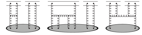
Figure 1: These diagrams show the contributions to the evolution of $T^{(2)}$, the scattering amplitude for a set of two dipoles off an arbitrary target represented here by a gray disk. From left to right: a linear BFKL term proportional to $T^{(2)}$, a merging term proportional to $T^{(3)}$ responsible for saturation, and a splitting term proportional to $T$ responsible for fluctuations.

To begin with, let us recall the important points concerning the QCD evolution equations towards high energy. To the present knowledge (in the leading logarithmic approximation and in the large-$N_{c}$ limit), those equations give the energy evolution for the scattering amplitude $\left\langle T^{(k)}\right\rangle$ between a system of $k$ dipoles of transverse coordinates $(\mathbf{x}_{1},\mathbf{y}_{1}),\dots,(\mathbf{x}_{k},\mathbf{y}_{k})$ and a generic target. They include three different types of contributions it as shown in Fig. 1: BFKL ladders, gluon mergings responsible for saturation corrections, and gluon splitting corresponding to gluon-number fluctuations. Summing these contributions results in a infinite hierarchy of equations, containing Pomeron loops, in which the evolution of $\left\langle T^{(k)}\right\rangle$ depends on $\left\langle T^{(k)}\right\rangle$, $\left\langle T^{(k+1)}\right\rangle$ and $\left\langle T^{(k-1)}\right\rangle$, coming respectively from the three types of contributions discussed previously.

The solutions of this hierarchy are not yet known and it is useful to deal with a simplified version of it. If we integrate out the impact-parameter dependence by performing a coarse-graining approximation it , we can Fourier transform the set of equations to momentum space ($r\rightarrow k$). The resulting hierarchy becomes equivalent to the following Langevin equation

$$\partial_{Y}T(k,Y)=\bar{\alpha}\int_{0}^{\infty}\frac{dp^{2}}{p^{2}}\,\left[\frac{p^{2}T(p,Y)-k^{2}T(k,Y)}{\left|p^{2}-k^{2}\right|}+\frac{k^{2}T(k,Y)}{\sqrt{4p^{4}+k^{4}}}\right]-\bar{\alpha}T^{2}(k,Y)+\bar{\alpha}\sqrt{2\kappa\alpha_{s}^{2}T(k,Y)}\>\nu(k,Y),$$ (1)

where $\nu(k,Y)$ is a Gaussian white noise satisfying

$$\left\langle\nu(k,Y)\right\rangle=0\qquad\text{ and }\quad\left\langle\nu(k,Y)\nu(k^{\prime},Y^{\prime})\right\rangle=\frac{2}{\bar{\alpha}\pi}\delta\left(\log(k^{2}/k^{\prime 2})\right)\delta(Y-Y^{\prime}).$$ (2)

The factor $\kappa$ present in front of the noise term comes from a local-noise approximation performed during the coarse graining.

• The linear part of equation (1) is the BFKL equation bfkl . Its solution $T_{\text{lin}}(k,Y)$ is a superposition of waves:

  $$T_{\text{lin}}(k,Y)=\int_{\frac{1}{2}-i\infty}^{\frac{1}{2}+i\infty}\frac{d\gamma}{2i\pi}\,e^{-\gamma[L-\bar{\alpha}v(\gamma)Y]}\,T_{0}(\gamma)$$ (3)

  where $L=\log(k^{2}/k_{0}^{2})$ and $T_{0}(\gamma)$ specifies the initial condition, characterised by the reference scale $k_{0}$. Each wave has a different speed $v(\gamma)$ given by

  $$v(\gamma)=\frac{\chi(\gamma)}{\gamma}\qquad\mbox{ with }\qquad\chi(\gamma)=2\psi(1)-\psi(\gamma)-\psi(1-\gamma)\ ,$$ (4)

  $\psi(\gamma)=\frac{d}{d\gamma}\log[\Gamma(\gamma)]$ being the digamma function.

• The equation (1) without the noise term is the BK equation. It has been shown mp to lie in the same universality class as the F-KPP equation fkpp which allowed analytical predictions. The non-linear term damps the growth of the amplitude predicted by the linear BFKL equation in such a way that the asymptotic solution $T_{\text{tw}}(k,Y)$ of the BK equation is a travelling wave of minimal speed $T_{\text{tw}}(L-\bar{\alpha}v_{c}Y).$ The minimal speed $v_{c}$ is obtained for a value of $\gamma$ that we shall denote $\gamma_{c}:$

  $$v_{c}=\min_{\gamma}\,v(\gamma)\equiv v(\gamma_{c})\quad\mbox{ with }\gamma_{c}\mbox{ solution of }\quad\frac{\chi(\gamma)}{\gamma}=\chi^{\prime}(\gamma)\ .$$ (5)

  For the BFKL kernel (4), one has $\gamma_{c}=0.6275$ and $v_{c}=4.883.$ From the position of the travelling wave one obtains the saturation scale $Q_{s}(Y)$, the momentum for which $T_{\text{tw}}$ is constant:

  $$T_{\text{tw}}(L-\bar{\alpha}v_{c}Y)\stackrel{{\scriptstyle L\gg\bar{\alpha}v_{c}Y}}{{=}}e^{-\gamma_{c}(L-\bar{\alpha}v_{c}Y)}=\left(\frac{k^{2}}{Q_{s}^{2}(Y)}\right)^{-\gamma_{c}}\mbox{ with }Q_{s}^{2}(Y)=k_{0}^{2}\ e^{\bar{\alpha}v_{c}Y}\ .$$ (6)

• The complete equation is a stochastic equation: it is the BK equation supplemented with a noise term which accounts for gluon-number fluctuations. It has been shown that, in the diffusive approximation where the integration in (1) is expressed as a second-order differential operator, Eq. (1) lies fluc in the same universality class as the sF-KPP equation

  $$\partial_{t}u(x,t)=\partial_{x}^{2}u(x,t)+u(x,t)-u^{2}(x,t)+\sqrt{2\lambda u(x,t)[1-u(x,t)]}\,\eta(x,t),$$ (7)

  with

  $$\left\langle\eta(x,t)\right\rangle=0\qquad\text{ and }\quad\left\langle\eta(x,t)\eta(x^{\prime},t^{\prime})\right\rangle=\delta(t-t^{\prime})\delta(x-x^{\prime}).$$ (8)

  In the analogy between (1) and (7), $\bar{\alpha}Y$ plays the role of time $t$ while the space variable $x$ is related to $L$ and $\lambda\propto\kappa\alpha_{s}^{2}$. The main analytical predictions concerning (1) are obtained from the study of the sF-KPP equation in the weak-noise limit. First, if one compares solutions of (1) with solutions of the BK equation, one obtains that each individual event is a travelling wave with a speed smaller than the one predicted from the BK equation. Then, if one consider a whole set of events, the main effect of the noise is to introduce dispersion in the position of different events. Physically, this means that the saturation scale fluctuates from one event to another and we can show, analytically (in the weak or strong noise limit) and numerically, that the average saturation scale $\bar{Q}_{s}^{2}(Y)$ grows as $\exp(\bar{\alpha}vY)$ with $v<v_{c}$ and that the dispersion of $\log(Q_{s}^{2}(Y))$ around that average value increases like $\sqrt{Y}$ as expected from a random-walk process.

III The probability distribution of the stochastic saturation scale

The saturation scale being a stochastic variable, it is characterised by a probability distribution. Let us call $P(\rho_{s})$ the probability distribution for the variable $\rho_{s}=\log(Q_{s}^{2}(Y)/k_{0}^{2}).$ From general arguments it was first inferred that $P(\rho_{s})$ should be Gaussian with an average value $\langle\rho_{s}\rangle=\log(\bar{Q}_{s}^{2}(Y)/k_{0}^{2})=\bar{\alpha}vY$ and a variance $\sigma^{2}=\bar{\alpha}DY,$ with $v$ and $D$ are coefficients characterising the speed and dispersion of the travelling wavefronts. This was then used extensively in the literature fluc ; it ; himst ; ims . Recently, the cumulants $\kappa_{n}$ of the distribution have been computed. The first cumulant $\kappa_{1}=\langle\rho_{s}\rangle$ is the average value of $\rho_{s}$ and the second cumulant $\kappa_{2}=\sigma^{2}$ is the variance of the distribution. In the Gaussian case higher-order cumulants are zero. The calculation of Brunet:2005bz showed that this was not the case: they find that higher-order cumulants are proportional to the second cumulant. To summarise, one has

$$\kappa_{1}=\langle\rho_{s}\rangle=\bar{\alpha}vY\ ,\hskip 28.45274pt\kappa_{2}=\sigma^{2}=\bar{\alpha}DY\ ,\hskip 28.45274pt\kappa_{n}=\frac{3\gamma_{c}^{2}}{\pi^{2}}\frac{n!\zeta(n)}{\gamma_{c}^{n}}\sigma^{2}\ ,$$ (9)

where $\zeta(n)$ is the Riemann Zeta function. Note that these results are valid in the high-energy limit $\gamma_{c}\sigma^{2}\gg 1$.

In the weak-noise ($\alpha_{s}^{2}\ll 1$) limit in which the results were obtained, one has

$$v=v(\gamma_{c})-\frac{\pi^{2}\gamma_{c}^{2}v^{\prime\prime}(\gamma_{c})}{\log^{2}(1/\alpha_{s}^{2})}\left(1-\frac{3\log[\log(1/\alpha_{s}^{2})]}{\log(1/\alpha_{s}^{2})}\right)\qquad\text{ and }\quad D=\frac{\pi^{4}\gamma_{c}v^{\prime\prime}(\gamma_{c})}{3\log^{3}(1/\alpha_{s}^{2})}\ .$$ (10)

But the fact that $\langle\rho_{s}\rangle$ and $\sigma^{2}$ are proportional to $Y$ is believed to be more general. This has been shown by an analytical study of the strong noise limit strong and it is confirmed by numerical simulations simul ; simul2 for arbitrary values of the noise strength (see also simul3 for related numerical studies). One observes that, when the noise strength increases, the speed of the wave $v$ decreases and the dispersion coefficient $D$ increases. In what follows, we shall therefore keep $v$ and $D$ as parameters.

III.1 Analytical results

In this section, we compute the probability distribution $P(\rho_{s})$ from the cumulants. Our starting point is the generating function for the moments of $P(\rho_{s})$

$$\left\langle e^{\lambda\rho_{s}}\right\rangle=\int_{-\infty}^{\infty}d\rho_{s}\,e^{\lambda\rho_{s}}\,P(\rho_{s})\ .$$ (11)

The cumulants generating function then reads

$$\log\left\langle e^{\lambda\rho_{s}}\right\rangle=\sum_{n>0}\frac{\kappa_{n}\lambda^{n}}{n!}=\langle\rho_{s}\rangle\lambda+\frac{3\gamma_{c}^{2}}{\pi^{2}}\sigma^{2}\sum_{n=2}^{\infty}\frac{\zeta(n)\lambda^{n}}{\gamma_{c}^{n}}\ .$$ (12)

If we use the following integral representation of the Zeta function

$$\zeta(n)=\frac{1}{\Gamma(n)}\int_{0}^{\infty}du\,\frac{u^{n-1}}{e^{u}-1},$$ (13)

we are able to compute analytically the cumulants generating function (12)

$$\log\left\langle e^{\lambda\rho_{s}}\right\rangle=\langle\rho_{s}\rangle\lambda+\frac{3\gamma_{c}^{2}}{\pi^{2}}\sigma^{2}\frac{\lambda}{\gamma_{c}}\int_{0}^{\infty}du\,\frac{e^{\lambda u/\gamma_{c}}-1}{e^{u}-1}=\langle\rho_{s}\rangle\lambda-\frac{3\gamma_{c}\sigma^{2}}{\pi^{2}}\lambda\left[\gamma_{E}+\psi\left(1-\frac{\lambda}{\gamma_{c}}\right)\right],$$ (14)

where $\gamma_{E}\approx 0.577216$ is the Euler constant.We can then inverse the Laplace transform in (11) to obtain the probability distribution ($c<\gamma_{c}$)

$$P(\rho_{s})=\int_{c-i\infty}^{c+i\infty}\frac{d\lambda}{2i\pi}\,\exp\left\{-\lambda z-b\lambda\left[\gamma_{E}+\psi\left(1-\frac{\lambda}{\gamma_{c}}\right)\right]\right\}\ .$$ (15)

where we have introduced

$$z=\rho_{s}-\langle\rho_{s}\rangle=\log\left(\frac{Q_{s}^{2}}{\bar{Q}_{s}^{2}}\right)\ ,\hskip 28.45274ptb=\frac{3\gamma_{c}\sigma^{2}}{\pi^{2}}\ .$$ (16)

$z$ is the distance of the saturation scale to its average value, and $b$ is a convenient redefinition of the variance. To evaluate further the probability distribution $P(\rho_{s})$, we shall perform the integration over $\lambda$ in the saddle point approximation. One finds that the saddle point $\tilde{\lambda}\equiv\gamma_{c}(1-\tilde{\varepsilon})$ has to satisfy

$$z+b\left[\gamma_{E}+\psi(\tilde{\varepsilon})-(1-\tilde{\varepsilon})\psi^{(1)}(\tilde{\varepsilon})\right]=0\ ,$$ (17)

where $\psi^{(n)}(x)$ is the polygamma function defined as $\frac{d^{n}}{dx^{n}}\psi(x)$. The probability distribution is then given by

$$P(\rho_{s})=\left\{\frac{12\sigma^{2}}{\pi}\left[\psi^{(1)}(\tilde{\varepsilon})-\frac{1-\tilde{\varepsilon}}{2}\psi^{(2)}(\tilde{\varepsilon})\right]\right\}^{-1/2}\exp\left[-\frac{3\sigma^{2}}{\pi^{2}}\gamma_{c}^{2}(1-\tilde{\varepsilon})^{2}\psi^{(1)}(\tilde{\varepsilon})\right].$$ (18)

Although Eq. (17) has no exact analytical solution, one can solve it in three interesting limits: $(i)$ $z/b\rightarrow 0$ which corresponds to $\tilde{\varepsilon}\rightarrow 1$; $(ii)$ $z/b\rightarrow\infty$ related to the limit $\tilde{\varepsilon}\rightarrow 0$; and $(iii)$ $z/b\rightarrow-\infty$ equivalent to the limit $\tilde{\varepsilon}\rightarrow\infty$. We detail these limits hereafter.

1. When $z/b\rightarrow 0$ or equivalently $|z|\ll\gamma_{c}\sigma^{2}$. Eq. (17) becomes

   $$\frac{z}{b}+\left[\gamma_{E}+\psi(1)-2(1-\tilde{\varepsilon})\psi^{(1)}(1)\right]=0\qquad\Rightarrow\qquad\tilde{\varepsilon}=1-\frac{3z}{\pi^{2}b}\ ,$$ (19)

   where we have used $\psi(1)=-\gamma_{E}$ and $\psi^{(1)}(1)=\pi^{2}/6$. After replacement in (18) we get

   $$P(\rho_{s})\approx\frac{1}{\sqrt{2\pi\sigma^{2}}}\left[1-\frac{9\zeta(3)}{\pi^{2}}\frac{z}{\gamma_{c}\sigma^{2}}\right]\exp\left(-\frac{z^{2}}{2\sigma^{2}}\right).$$ (20)

   We kept the first subleading term to show that this distribution has a maximum for the constant value

   $$z\approx\frac{-9\zeta(3)}{\pi^{2}\gamma_{c}}\approx-1.75.$$ (21)

   The most probable value for the saturation scale is therefore not the average value $\langle\rho_{s}\rangle$. For asymptotically large energies, we recover

   $$P(\rho_{s})\approx\frac{1}{\sqrt{2\pi\sigma^{2}}}\exp\left(-\frac{z^{2}}{2\sigma^{2}}\right)$$ (22)

   The probability distribution of fronts is Gaussian around the average. We shall discuss later on the fact that this is the dominant behaviour at high-energy which justifies the use of a Gaussian distribution in fluc ; it ; himst ; ims .

2. When $z/b\rightarrow+\infty$ or equivalently $z\gg\gamma_{c}\sigma^{2}$. We are sensitive to small values of $\tilde{\varepsilon}$. One can thus simplify Eq. (17) and obtain

   $$-\left(\frac{z}{b}\right)+\frac{1}{\tilde{\varepsilon}}+\frac{1-\tilde{\varepsilon}}{\tilde{\varepsilon}^{2}}+\frac{\pi^{2}}{6}=0\ ,\qquad\Rightarrow\qquad\tilde{\varepsilon}=\sqrt{\frac{3}{\pi^{2}}\frac{\gamma_{c}\sigma^{2}}{z}}\left(1+\frac{\gamma_{c}\sigma^{2}}{4z}\right).$$ (23)

   After a bit of algebra, this turns into the following limit for the probability distribution

   $$P(\rho_{s})\approx\frac{3^{1/4}}{2\pi\sigma}\left(\frac{\gamma_{c}\sigma^{2}}{z}\right)^{3/4}\exp\left[-\gamma_{c}z\left(1-2\sqrt{\frac{3}{\pi^{2}}\frac{\gamma_{c}\sigma^{2}}{z}}\right)\right]\ .$$ (24)

   This corresponds to a power-law tail $P(\rho_{s})\sim(Q_{s}/\bar{Q}_{s})^{-2\gamma_{c}}$ at very large $Q_{s}$.

3. When $z/b\rightarrow-\infty$ or equivalently $z\ll-\gamma_{c}\sigma^{2}$. We have $\tilde{\varepsilon}\to\infty$, and Eq. (17) turns into

   $$\frac{z}{b}+\gamma_{E}+\log(\tilde{\varepsilon})+1-\frac{1}{\tilde{\varepsilon}}=0\qquad\Rightarrow\qquad\tilde{\varepsilon}=\exp\left(-\frac{\pi^{2}}{3}\frac{z}{\gamma_{c}\sigma^{2}}-1-\gamma_{E}\right)+1.$$ (25)

   The probability (18) is then found to be

   $$P(\rho_{s})\approx\sqrt{\frac{\pi}{6}}\frac{1}{\sigma}\exp\left\{-\frac{\pi^{2}}{6}\frac{z}{\gamma_{c}\sigma^{2}}-\frac{1+\gamma_{E}}{2}-\frac{3\gamma_{c}^{2}\sigma^{2}}{\pi^{2}}\left[\exp\left(-\frac{\pi^{2}}{3}\frac{z}{\gamma_{c}\sigma^{2}}-1-\gamma_{E}\right)-\frac{1}{2}\right]\right\}.$$ (26)

   This is a Gumbel distribution, which goes to zero very fast when $z\ll-\gamma_{c}\sigma^{2}$.

As a function of $z$ starting from $z=-\infty,$ the transition between the regime (26) and the regime (22) happens for $z=-\gamma_{c}\sigma^{2}$ and the transition between the regime (22) and the regime (24) happens for $z=\gamma_{c}\sigma^{2}.$ For those two points, $\rho_{s}=\langle\rho_{s}\rangle\pm\gamma_{c}\sigma^{2},$ the probability is of order $e^{-\gamma_{c}^{2}\sigma^{2}}/\sigma$ which is very small. This means that the probability $P(\rho_{s})$ is not Gaussian only for very improbable fluctuations. To describe the bulk of the events, the Gaussian distribution (22) is a good approximation.

III.2 Numerical results

In this section, we shall compare the analytical prediction (18) derived in the previous section with the numerical simulation of (1) introduced in simul . To fix things properly we need first to recall a few points from simul . In that study, we start with a fixed initial condition and evolve numerically the QCD Langevin equation with different realisation of the noise term (the precise method used to solve the equation is not important for our purposes here, so we refer to simul for details). The momentum $k$ is discretised in bins of $L=\log(k^{2}/k_{0}^{2})$ between $L_{\text{min}}$ and $L_{\text{max}}$. Hence, the numerical simulations of (1) results in a set of events $T_{i}(L_{j},Y)$, with $i=1,\dots,n_{\text{ev}}$, i.e., for each event $i$, we get the rapidity evolution of the amplitude in each momentum bin.

As expected from the analytical study of (1) in the weak-noise limit, the numerical studies have confirmed that each event is a travelling wave whose speed decreases when the strength of the fluctuations increases. Also, at large rapidities, the position of the wavefront shows a dispersion proportional to $\sqrt{Y}$ if one consider a whole set of events. Practically, those results can be summarised by saying that, for the $i$th event, we have

$$T_{i}(L,Y)=T_{i}(L-L_{s,i}(Y))\qquad\text{ with }\quad L_{s}\equiv\rho_{s}=\log(Q_{s}^{2}(Y)/k_{0}^{2}).$$ (27)

The position $L_{s,i}(Y)$ of the wavefront for one event can be extracted from the numerical simulations by solving $T_{i}(L,Y)=T_{0}$ for a fixed $T_{0}$ (here, we adopted $T_{0}=0.2$) and for different values of the rapidity. By measuring (the logarithm of) the saturation scale, one can obtain its statistical distribution. More precisely, for each rapidity, we construct a histogram by counting, for a set of events, the number of event for which the saturation scale is in each momentum bin.

In order to compare with the analytical predictions, we shall, instead of the histogram for $\rho_{s}$, use the distribution for $z=\rho_{s}-\langle\rho_{s}\rangle$. Normalised in such a way that its integral is 1, it is directly comparable with (18) if one fixes the dispersion parameter. For the latter we adopt the value computed numerically from the histogram of $\rho_{s}$ or $z$. In other words, we fix the two lowest-order cumulants $\langle\rho_{s}\rangle$ and $\sigma^{2}$, and compare the resulting analytical and numerical probability distribution at different rapidities.

The results are shown in Fig. 2, for two sets of 10000 events taken from simul . Those two sets corresponds to different values of the noise strength $\tilde{\kappa}\!=\!10\pi\kappa/N_{c}^{2}\!=\!1$ and $5$, the value of $\bar{\alpha}$ being fixed to 0.2. For both cases, we show the probability distribution for rapidities $Y=20$, $30$ and $40$. Those rapidities are in the region where the travelling wavefront has reached its asymptotic behaviour and the dispersion of the wavefronts is proportional to $\sqrt{Y}$ as expected.

It is obvious from Fig. 2 that the agreement is excellent with predictions from (18). One can see that, in the bulk of the distribution, the probability is Gaussian, up to a shift of the maximum to a negative value which is consistent with (21). We also observe that the probability falls very fast in the infrared and has a tail which favours fluctuations to large values of the saturation momentum. However, the deviations from a Gaussian behaviour only appear for events with a very small probability.

Figure 2: Comparison of the probability distribution (18) as a function of $z=\rho_{s}-\langle\rho_{s}\rangle$ with results from numerical simulations with $\tilde{\kappa}=1$ (top) and $\tilde{\kappa}=5$ (bottom). The comparisons are made for $Y=20$, $30$, $40$, from left to right.

IV Consequences for the physical scattering amplitude

We shall now compute the behaviour of the average scattering amplitudes $\left\langle T(\rho,Y)\right\rangle$ where $\rho=\log[1/(k_{0}^{2}r^{2})]$, using the probability distribution obtained in the previous section. For simplicity, we consider the amplitude in coordinate space. The average amplitude can be directly computed from the probability $P(\rho_{s})$ using

$$\left\langle T(\rho,Y)\right\rangle=\int_{-\infty}^{\infty}d\rho_{s}\,P(\rho_{s})T(\rho-\rho_{s}),$$ (28)

where $T(\rho-\rho_{s})$ describe the event-by-event amplitude which features the travelling-wave property w.r.t. the saturation scale $\rho_{s}$. Inserting the probability distribution (15) into (28) and using the Mellin representation

$$T(\rho)=\int\frac{d\lambda}{2i\pi}\,e^{-\lambda\rho}\,\tilde{T}(\lambda),$$ (29)

we obtain for the physical amplitude

$$\left\langle T(\rho,Y)\right\rangle=\int\frac{d\lambda}{2i\pi}\,\tilde{T}(\lambda)\,\exp\left\{-\lambda Z-b\lambda\left[\gamma_{E}+\psi\left(1-\frac{\lambda}{\gamma_{c}}\right)\right]\right\}.$$ (30)

We have introduced the convenient variable

$$Z=\rho-\langle\rho_{s}\rangle=-\log\left(r^{2}\bar{Q}_{s}^{2}(Y)\right)\ .$$ (31)

Since the function $\tilde{T}(\lambda)$ is slowly varying the remaining integration will basically be sensitive to the same saddle point (17) as for the computation of the probability. The main difference lies in the fact that, because of the unitarity constraint, $\tilde{T}(\lambda)$ has a pole in $\gamma=0$. Hence, in order to get relevant expressions in the different physical limits, the following assumption for the event-by-event wavefront is sufficient:

$$T(\rho-\rho_{s})=\begin{cases}1&\rho\leq\rho_{s}\\ \exp\left[-\gamma_{0}(\rho-\rho_{s})\right]&\rho>\rho_{s}\end{cases}\qquad\qquad\Rightarrow\qquad\tilde{T}(\lambda)=\frac{1}{\lambda}+\frac{1}{\gamma_{0}-\lambda}.$$ (32)

This satisfies both the travelling-wave property (6) and unitarity requirements. The exponent $\gamma_{0}$ can be chosen between $\gamma_{c}$ and 1.

We can now introduce (32) in (30) and we get

$$\left\langle T(\rho,Y)\right\rangle=\int_{c-i\infty}^{c+i\infty}\frac{d\lambda}{2i\pi}\,\frac{\gamma_{0}}{\lambda(\gamma_{0}-\lambda)}\exp\left\{-\lambda Z-b\lambda\left[\gamma_{E}+\psi\left(1-\frac{\lambda}{\gamma_{c}}\right)\right]\right\},$$ (33)

where the contour of integration is now restricted to values of $c$ such that $0<c<\gamma_{c}$. The remaining integration over $\lambda$ can be computed in the saddle-point approximation and the condition (17) is still appropriate for (33). Again, the physical picture arises when we consider the three different limits $|Z|\ll\gamma_{c}\sigma^{2}$, $Z\gg\gamma_{c}\sigma^{2}$ and $Z\ll-\gamma_{c}\sigma^{2}$, which we detail hereafter.

1. Case $Z\gg\gamma_{c}\sigma^{2}$: as for the computation of the probability, the saddle point is obtained by expansion around $\tilde{\varepsilon}\to 0$ or $\tilde{\lambda}\to\gamma_{c}$ and the same result is obtained, up to an extra factor $(\gamma_{0}-\tilde{\lambda})^{-1}$. For $\gamma_{0}>\gamma_{c}$, this leads to

   $$\left\langle T(\rho,Y)\right\rangle\approx\frac{3^{1/4}}{2\pi\sigma(\gamma_{0}-\gamma_{c})}\left(\frac{\gamma_{c}\sigma^{2}}{Z}\right)^{3/4}\exp(-\gamma_{c}Z).$$ (34)

   If $\gamma_{0}=\gamma_{c}$, we get an additional contribution from the pole

   $$\left\langle T(\rho,Y)\right\rangle\approx\frac{3^{-1/4}}{2\gamma_{c}\sigma}\left(\frac{\gamma_{c}\sigma^{2}}{Z}\right)^{1/4}\exp(-\gamma_{c}Z).$$ (35)

2. Case $Z\ll-\gamma_{c}\sigma^{2}$: this case is slightly more intricate. Indeed, since $\tilde{\lambda}\to-\infty$, the contour of integration must first be moved towards $c=\tilde{\lambda}$. The integration therefore receives a contribution of $1$ coming from the pole at $\lambda=0$. The final result reads

   $$\left\langle T(\rho,Y)\right\rangle\approx 1-\sqrt{\frac{\pi}{6}}\frac{1}{\gamma_{c}\sigma}\exp\left\{\frac{\pi^{2}}{2}\frac{Z}{\gamma_{c}\sigma^{2}}+\frac{3}{2}(1+\gamma_{E})-\frac{3\gamma_{c}^{2}\sigma^{2}}{\pi^{2}}\left[\exp\left(-\frac{\pi^{2}}{3}\frac{Z}{\gamma_{c}\sigma^{2}}-1-\gamma_{E}\right)-\frac{1}{2}\right]\right\}.$$ (36)

3. Case $|Z|\ll\gamma_{c}\sigma^{2}$: for that last case, we have to distinguish between two possibilities: $Z>0$ and $Z<0$. Let us start with the positive values of $Z$: as for the computation of the probability, this situation is sensitive to $\tilde{\lambda}\to 0$. Hence, we need to properly take into account the prefactor $\lambda^{-1}=\exp[-\log(\lambda)]$. This gives an additional contribution $-\tilde{\lambda}^{-1}$ to the saddle point equation which becomes

   $$Z-\sigma^{2}\tilde{\lambda}-\frac{1}{\tilde{\lambda}}=0\qquad\Rightarrow\qquad\tilde{\lambda}=\frac{Z}{2\sigma^{2}}+\frac{1}{2\sigma^{2}}\sqrt{Z^{2}+4\sigma^{2}}.$$ (37)

   If, in addition, one requires $Z\gg\sigma$, we recover $\tilde{\lambda}=Z/\sigma^{2}$ as for the computation of the probability. The average amplitude is then the same as the probability, up to an extra factor $\lambda^{-1}$, which gives

   $$\left\langle T(\rho,Y)\right\rangle\approx\frac{1}{\sqrt{2\pi}}\frac{\sigma}{Z}\exp\left(-\frac{Z^{2}}{2\sigma^{2}}\right).$$ (38)

   For the case where $Z$ is negative, we first move the integration contour on the left side of the pole at $\lambda=0$ which gives a contribution of $1$ and the remaining integration is computed in the same way as for positive $Z$. That is, for $-\gamma_{c}\sigma^{2}\ll Z\ll-\sigma$, we obtain

   $$\left\langle T(\rho,Y)\right\rangle\approx 1-\frac{1}{\sqrt{2\pi}}\frac{\sigma}{|Z|}\exp\left(-\frac{Z^{2}}{2\sigma^{2}}\right),$$ (39)

   where we have explicitly emphasised the sign of the second term. The two results (38) and (39) can be summarised in only one formula:

   $$\left\langle T(\rho,Y)\right\rangle\approx\frac{1}{2}\,{\rm erfc}\left(\frac{Z}{\sqrt{2}\sigma}\right),$$ (40)

   where ${\rm erfc}(x)$ is the complementary error function.

Figure 3: Comparison of the physical amplitude $\left\langle T(\rho,Y)\right\rangle$ plotted as a function of $Z/\sigma$ and the error function obtained as the asymptotic behaviour.

The results (35), $\eqref{eq:average_small}$ and (40) call for a number of comments. The most important one is that (for very high energies such that $\gamma_{c}\sigma^{2}\gg 1$) one recovers the error function as expected previously in the literature fluc ; it ; himst ; ims and the scattering amplitude satisfies diffusive scaling as it depends only on the ratio $Z/\sigma$. This result is valid in a very large window around the average saturation scale ($Z\ll\gamma_{c}\sigma^{2}$). Since this can directly be derived from the front (32) convoluted with the Gaussian probability distribution (22), this means that it is sufficient to consider a Gaussian distribution in order to compute the scattering amplitudes at high-energy. In addition, the error function fully comes from $\rho<\rho_{s}$ in (32), which proves the expected result himst ; ims that the amplitude is dominated, up to very large values of $\rho$, by fronts at saturation i.e. by black spots. Finally, let us notice that our argument does not depend on the particular choice for the event-by-event front. Indeed, the pole in $\lambda^{-1}$ comes from the saturated part of (32) and thus the condition that the event-by-event amplitude satisfies unitarity is sufficient to obtain (40).

To illustrate that behaviour, we have computed from (28) the amplitude obtained using an event-by-event front $\Theta(\rho_{s}-\rho)$ ($\Theta(x)$ being the Heaviside function). We plot on Fig. 3 the result for different values of $\sigma$ as a function of the high-energy scaling variable $Z/\sigma$. We clearly observe that when $\sigma$ increases (i.e. when energy increases), we converge to the universal error function (40).

The behaviour in the far tail $Z\gg\gamma_{c}\sigma^{2}$ is also quite interesting. Indeed, if we adopt $\gamma_{0}=\gamma_{c}$, the amplitude (35) decreases as $\exp(-\gamma_{c}Z)$ as expected, but it receives contributions both from the event-by-event amplitude and from the probability distribution. Finally, deep inside the saturation region we obtain that the amplitude reaches the unitarity limit like $1-c_{1}\exp[-c_{2}(r\bar{Q}_{s})^{2c_{3}}]$ where $c_{1}$, $c_{2}$ and $c_{3}$ can be read on Eq. (36).

V Conclusion and discussion

Let us now summarise the results obtained in this paper. First, we have shown that it is possible to compute the probability distribution for the position of the wavefront satisfying the stochastic F-KPP equation, which corresponds to the saturation scale in QCD. Our starting point is the cumulants of this distribution computed previously in Brunet:2005bz . The probability distribution is computed in a saddle point approximation. This allows us to compute its leading behaviour in the vicinity of the average saturation scale $\langle\rho_{s}\rangle$ where the probability is Gaussian, as well as for improbable events far above or below $\langle\rho_{s}\rangle$.

Then, we have checked that the predictions for the probability distribution are in good agreement with the results obtained from the numerical simulations of the QCD Langevin equation (1), once one fixes the average position and its dispersion from their numerical values. Since the numerical simulations are not obtained in the weak noise limit and not directly for the sF-KPP equation, this proves once again that the probability distribution derived in this paper has some universal properties.

From the probability distribution we are able to deduce the physical scattering amplitude. Again, we have considered the same interesting asymptotic behaviours as for the probability distribution: the vicinity of the average saturation scale, deep inside the saturation regime or in the dilute domain. Within this analysis, the most important result is that at high-energy the probability distribution can be considered as Gaussian over an very large domain $|z|\ll~{}\gamma_{c}\sigma^{2}~{}\propto~{}Y$. As a consequence the scattering amplitudes are dominated by events which are at saturation.

This validates the approach adopted in Refs. himst ; ims , and leads to the fact that scattering amplitudes scale as a function of $\log[r^{2}\bar{Q}_{s}^{2}(Y)]/\sqrt{Y}$, a property which is known as diffusive scaling and may have important consequences on LHC physics. The domain over which the probability distribution may be considered as Gaussian extends over a region of $\rho_{s}$ which satisfies $|\rho_{s}-\langle\rho_{s}\rangle|\ll\gamma_{c}\sigma^{2}$. As the dispersion $\sigma$ grows like $\sqrt{Y}$, this domain becomes larger and larger with increasing rpidity. The same argument holds for the region $|Z|\ll\gamma_{c}\sigma^{2}$ for which the scattering amplitude satisfies diffusive scaling. Those facts also corroborate the result from strong that, in the strong-fluctuation limit, the scattering amplitude is given by the error function (40), which is a superposition of Heaviside functions with a Gaussian distribution.

Of course, the analytical behaviour of the cumulants associated with the distribution of $\rho_{s}$ for any value of $\alpha_{s}$ and in the case of the full QCD equation (1) still remains an open question. However, our analytical and numerical results show that they are compatible with a universal probability distribution. This deserves more detailed studies.

- (1) S. Munier and R. Peschanski, Phys. Rev. Lett. 91, (2003) 232001; Phys. Rev. D69, (2004) 034008; Phys. Rev. D70, (2004) 077503.
- (2) I. Balitsky, Nucl. Phys. B463 (1996) 99; Y. V. Kovchegov, Phys. Rev. D60 (1999) 034008; Phys. Rev. D61 (2000) 074018.
- (3) R. A. Fisher, Ann. Eugenics 7 (1937) 355; A. Kolmogorov, I. Petrovsky, and N. Piscounov, Moscou Univ. Bull. Math. A1 (1937) 1.
- (4) A. H. Mueller and A. I. Shoshi, Nucl. Phys. B 692 (2004) 175.
- (5) E. Iancu, A. H. Mueller and S. Munier, Phys. Lett. B 606 (2005) 342; S. Munier, Nucl. Phys. A 755 (2005) 622.
- (6) E. Iancu and D. N. Triantafyllopoulos, Nucl. Phys. A 756 (2005) 419; Phys. Lett. B 610 (2005) 253.
- (7) E. Iancu, G. Soyez and D. N. Triantafyllopoulos, Nucl. Phys. A 768 (2006) 194.
- (8) E. Brunet, B. Derrida, A. H. Mueller and S. Munier, arXiv:cond-mat/0512021.
- (9) G. Soyez, Phys. Rev. D 72 (2005) 016007.
- (10) Y. Hatta, E. Iancu, C. Marquet, G. Soyez and D. N. Triantafyllopoulos, Nucl. Phys. A 773 (2006) 95.
- (11) E. Iancu, C. Marquet and G. Soyez, arXiv:hep-ph/0605174.
- (12) L. N. Lipatov, Sov. J. Nucl. Phys. 23, (1976) 338; E. A. Kuraev, L. N. Lipatov and V. S. Fadin, Sov. Phys. JETP 45, (1977) 199; I. I. Balitsky and L. N. Lipatov, Sov. J. Nucl. Phys. 28, (1978) 822.
- (13) C. Marquet, R. Peschanski and G. Soyez, Phys. Rev. D 73 (2006) 114005.
- (14) R. Enberg, K. Golec-Biernat and S. Munier, Phys. Rev. D 72 (2005) 074021.
- (15) N. Armesto and J. G. Milhano, Phys. Rev. D 73 (2006) 114003.