Isospin symmetry breaking of K and K* mesons

Abstract

We use the method of QCD sum rules to investigate the isospin symmetry breaking of K and K* mesons. The electromagnetic effect, difference between up and down current-quark masses and difference between up and down quark condensates are important. We perform sum rule analyses of their masses and decay constant differences, which are consistent with experimental values. Our results yield $\Delta f_{K}=f_{K^{0}}-f_{K^{\pm}}=1.5$ MeV.

I Introduction

QCD has an approximate flavor symmetry which is determined by the pattern of the quark masses. Isospin symmetry in particular holds to a high accuracy. This is because the scale is set by $(m_{u}-m_{d})/\Lambda_{\chi}$, where $m$’s are current quark masses, while $\Lambda_{\chi}$ is the chiral symmetry breaking scale around 1 GeV. Because of this small hadronic isospin violations, the electromagnetic effect becomes important in order to understand the isospin symmetry breaking Das:1967it ; Fujikawa:1974wa ; Scorzato:2004da . There are many papers suggesting that the electromagnetic effect is dominant in the mass splitting of pions Bardeen:1988zw ; Duncan:1996xy .

Therefore, to study the isospin symmetry breaking, it is necessary to consider both the hadronic isospin violations and the electromagnetic effect. In this paper, we study the isospin symmetry breaking of $K$ and $K^{*}$ ($J^{P}=0^{+}$) mesons in the QCD sum rule. This work is an extension of the previous one for the $\pi$ and $\rho$ mesons Zhu:1997mp .

One can calculate the hadronic effect due to the different $up$ and $down$ current-quark masses and condensates. While for the electromagnetic effect, we follow the procedure in Ref. Kisslinger:1994me . They constructed a gauge invariant electromagnetic two-point function for the heavy-light quark systems.

This paper is organized as follows. In section 2, we derive the QCD sum rules for the $K$ and $K^{*}$ mesons. In section 3, we discuss our numerical results of their masses, decay constants and differences. We find that they are consistent with the experimental values. Section 4 is a summary.

II QCD Sum Rules for $K$ and $K^{*}$ Mesons

For the past decades QCD sum rule has proven to be a powerful and successful non-perturbative method Shifman:1978bx ; Reinders:1984sr . In sum rule analyses, we consider two-point correlation functions:

$$\Pi_{\mu\nu}(q^{2})\, \equiv \,i\int d^{4}xe^{iqx}\langle 0|T\eta_{\mu}(x){\eta_{\nu}^{\dagger}}(0)|0\rangle$$

$$= \Pi(q^{2})(q_{\mu}q_{\nu}-q^{2}g_{\mu\nu})+\Pi_{1}(q^{2})q_{\mu}q_{\nu}\,,$$

where for $K$ meson

$$\eta_{\mu}^{(K)}=\bar{q}_{1}\gamma_{\mu}\gamma_{5}q_{2}\,,$$ (2)

and for the vector $K^{*}$ meson

$$\eta_{\mu}^{(K^{*})}=\bar{q}_{1}\gamma_{\mu}q_{2}\,.$$ (3)

Here these currents may couple to particles $K$ and $K^{*}$ through

$$\langle 0|\eta_{\mu}^{(K)}(0)|K(p)\rangle = ip_{\mu}f_{K}\,,$$

$$\langle 0|\eta_{\mu}^{(K^{*})}(0)|K^{*}(p)\rangle = f_{K^{*}}m_{K^{*}}\epsilon_{\mu}^{K^{*}}\,.$$

Here $p_{\mu}$ is the four momentum carried by the initial meson, $f_{K}$ and $f_{K^{*}}$ are the decay constants of $K$ and $K^{*}$ respectively, $m_{K^{*}}$ is the mass of $K^{*}$, and $\epsilon_{\mu}^{K^{*}}$ is the polarization vector of $K^{*}$. In the OPE, $\Pi(q^{2})$ can be divided into two parts: the hadronic part and the contributions from the electromagnetic effects. The hadronic part for $K$ and $K^{*}$ have been calculated in the original work of the QCD sum rule Shifman:1978bx ; Ball:2005vx .

For the charge neutral current, like $K^{0}$ and $K^{*0}$, we can change the gluons in QCD to the photons up to the order of $\alpha_{e}$ ($\equiv e^{2}/4\pi$), and easily calculate electromagnetic contributions. For the charged current, like $K^{\pm}$ and $K^{*\pm}$, the calculation of electromagnetic contributions is slightly more complicated. If we simply change gluons to photons, the result is not gauge invariant. To solve this problem, we follow the procedure in Ref. Kisslinger:1994me . Expanding to order $\alpha_{e}$, the currents become (Fig. 1)

$$\eta_{\mu}^{(K)}(q^{2}) = \bar{q}_{1}\gamma_{\mu}\gamma_{5}q_{2}-ee_{T}~{}\bar{q}_{1}(q-k_{1})~{}~{}\gamma_{\mu}\gamma_{5}\frac{(k_{1}-k_{2})_{\nu}}{(k_{1}-k_{2})^{2}}~{}~{}A_{\nu}(k_{1}-k_{2})~{}~{}q_{2}(k_{2})\,,$$ (4)

$$\eta_{\mu}^{(K^{*})}(q^{2}) = \bar{q}_{1}\gamma_{\mu}q_{2}-ee_{T}~{}\bar{q}_{1}(q-k_{1})~{}~{}\gamma_{\mu}\frac{(k_{1}-k_{2})_{\nu}}{(k_{1}-k_{2})^{2}}~{}~{}A_{\nu}(k_{1}-k_{2})~{}~{}q_{2}(k_{2})\,,$$ (5)

where the normalized total charge of the meson is defined by $e_{T}\equiv e_{q_{1}}-e_{q_{2}}$, and takes $\pm 1$ for $K^{\pm}$ and $K^{*\pm}$.

Figure 1: The gauge invariant current up to order $\alpha_{e}$

We have performed the OPE calculation up to dimension six, which contains the four-quark condensates. The results are

$$\Pi_{K^{0}(\bar{K}^{0})} = -{1\over 4\pi^{2}}(1+{\alpha_{s}\over\pi})\ln{-q^{2}\over\mu^{2}}-{1\over 4\pi^{2}}{e_{d}^{2}+e_{s}^{2}\over 2}{\alpha_{e}\over\pi}\ln{-q^{2}\over\mu^{2}}$$

$$+{3\over 8\pi^{2}q^{2}}(m_{d}+m_{s})^{2}\ln{-q^{2}\over\mu^{2}}-{1\over q^{4}}(m_{d}\langle\bar{s}s\rangle+m_{s}\langle\bar{d}d\rangle)$$

$$+{1\over 12q^{4}}\langle{\alpha_{s}\over\pi}G^{2}\rangle-{352\pi\over 81q^{6}}\alpha_{s}\langle\bar{d}d\rangle\langle\bar{s}s\rangle-{44\pi\over 27q^{6}}\alpha_{e}e_{d}e_{s}(\langle{\bar{d}}d\rangle^{2}+\langle{\bar{s}}s\rangle^{2})\,,$$

$$\Pi_{K^{\pm}} = -{1\over 4\pi^{2}}(1+{\alpha_{s}\over\pi})\ln{-q^{2}\over\mu^{2}}-{1\over 4\pi^{2}}e_{u}e_{s}{\alpha_{e}\over\pi}\ln{-q^{2}\over\mu^{2}}$$

$$+{3\over 8\pi^{2}q^{2}}(m_{u}+m_{s})^{2}\ln{-q^{2}\over\mu^{2}}-{1\over q^{4}}(m_{u}\langle\bar{s}s\rangle+m_{s}\langle\bar{u}u\rangle)$$

$$+{1\over 12q^{4}}\langle{\alpha_{s}\over\pi}G^{2}\rangle-{352\pi\over 81q^{6}}\alpha_{s}\langle\bar{u}u\rangle\langle\bar{s}s\rangle-{44\pi\over 27q^{6}}\alpha_{e}e_{u}e_{s}(\langle{\bar{u}}u\rangle^{2}+\langle{\bar{s}}s\rangle^{2})\,,$$

$$\Pi_{K^{*0}(\bar{K}^{*0})} = -{1\over 4\pi^{2}}(1+{\alpha_{s}\over\pi})\ln{-q^{2}\over\mu^{2}}-{1\over 4\pi^{2}}{e_{d}^{2}+e_{s}^{2}\over 2}{\alpha_{e}\over\pi}\ln{-q^{2}\over\mu^{2}}$$

$$+{3\over 8\pi^{2}q^{2}}(m_{d}-m_{s})^{2}\ln{-q^{2}\over\mu^{2}}+{1\over q^{4}}(m_{d}\langle{\bar{s}}s\rangle+m_{s}\langle{\bar{d}}d\rangle)$$

$$+{1\over 12q^{4}}\langle{\alpha_{s}\over\pi}G^{2}\rangle+{32\pi\over 9q^{6}}\alpha_{s}\langle{\bar{d}}d\rangle\langle{\bar{s}}s\rangle-{32\pi\over 81q^{6}}\alpha_{s}(\langle{\bar{d}}d\rangle^{2}+\langle{\bar{s}}s\rangle^{2})$$

$$+{28\pi\over 27q^{6}}\alpha_{e}e_{d}e_{s}(\langle{\bar{d}}d\rangle^{2}+\langle{\bar{s}}s\rangle^{2})\,,$$

$$\Pi_{K^{*\pm}} = -{1\over 4\pi^{2}}(1+{\alpha_{s}\over\pi})\ln{-q^{2}\over\mu^{2}}-{1\over 4\pi^{2}}e_{u}e_{s}{\alpha_{e}\over\pi}\ln{-q^{2}\over\mu^{2}}$$

$$+{3\over 8\pi^{2}q^{2}}(m_{u}-m_{s})^{2}\ln{-q^{2}\over\mu^{2}}+{1\over q^{4}}(m_{u}\langle{\bar{s}}s\rangle+m_{s}\langle{\bar{u}}u\rangle)$$

$$+{1\over 12q^{4}}\langle{\alpha_{s}\over\pi}G^{2}\rangle+{32\pi\over 9q^{6}}\alpha_{s}\langle{\bar{u}}u\rangle\langle{\bar{s}}s\rangle-{32\pi\over 81q^{6}}\alpha_{s}(\langle{\bar{u}}u\rangle^{2}+\langle{\bar{s}}s\rangle^{2})$$

$$+{\pi\over q^{6}}\alpha_{e}e_{T}^{2}\langle{\bar{u}}u\rangle\langle{\bar{s}}s\rangle+{28\pi\over 27q^{6}}\alpha_{e}e_{u}e_{s}(\langle{\bar{u}}u\rangle^{2}+\langle{\bar{s}}s\rangle^{2})\,.$$

In these equations, $u,d,s$ represent $u$, $d$ and $s$ quarks respectively. The couplings $e_{u}$, $e_{d}$ and $e_{s}$ are normalized by the unit electric charge $e$, and therefore, $e_{u}=2/3$ and $e_{d}=e_{s}=-1/3$. The quantities $\langle\bar{u}u\rangle$, $\langle\bar{d}d\rangle$ and $\langle\bar{s}s\rangle$ are dimension $D=3$ quark condensates, and $\langle g^{2}GG\rangle$ is a $D=4$ gluon condensate. We have assumed the vacuum dominance and factorization for the four quark condensates, for instance Shifman:1978bx ,

$$\langle 0|\bar{q}\gamma_{\mu}\gamma_{5}{\lambda^{a}\over 2}q\bar{q}\gamma^{\mu}\gamma_{5}{\lambda^{a}\over 2}q|0\rangle={16\over 9}\langle 0|\bar{q}q|0\rangle^{2}\,,$$

$$\langle 0|\bar{q}\sigma_{\mu\nu}\gamma_{5}{\lambda^{a}\over 2}q\bar{q}\sigma^{\mu\nu}\gamma_{5}{\lambda^{a}\over 2}q|0\rangle={16\over 3}\langle 0|\bar{q}q|0\rangle^{2}\,.$$

The difference $\Pi_{K^{0}}-\Pi_{K^{\pm}}$ determines the isospin symmetry breaking of $K$ meson, while the difference $\Pi_{K^{*0}}-\Pi_{K^{*\pm}}$ determines the isospin symmetry breaking of $K^{*}$ meson. If we consider that the difference between the $up$ and $down$ quark condensates is small and introduce the average condensate $\langle\bar{q}q\rangle=(\langle\bar{u}u\rangle+\langle\bar{d}d\rangle)/2$, we find

$$\Pi_{K^{0}}-\Pi_{K^{\pm}} \approx {1\over 8\pi^{2}}(2e_{u}e_{s}-e_{d}^{2}-e_{s}^{2}){\alpha_{e}\over\pi}\ln{-q^{2}\over\mu^{2}}-{3\over 8\pi^{2}q^{2}}(m_{u}+m_{d}+2m_{s})(m_{u}-m_{d})\ln{-q^{2}\over\mu^{2}}$$

$$+{1\over q^{4}}(m_{u}-m_{d})\langle\bar{s}s\rangle+{1\over q^{4}}m_{s}(\langle\bar{u}u\rangle-\langle\bar{d}d\rangle)$$

$$+{352\pi\over 81q^{6}}\alpha_{s}\langle\bar{s}s\rangle(\langle\bar{u}u\rangle-\langle\bar{d}d\rangle)+{44\pi\over 27q^{6}}\alpha_{e}(e_{u}-e_{d})e_{s}(\langle\bar{q}q\rangle^{2}+\langle\bar{s}s\rangle^{2})\,,$$

$$\Pi_{K^{*0}}-\Pi_{K^{*\pm}} \approx {1\over 8\pi^{2}}(2e_{u}e_{s}-e_{d}^{2}-e_{s}^{2}){\alpha_{e}\over\pi}\ln{-q^{2}\over\mu^{2}}-{3\over 8\pi^{2}q^{2}}(m_{u}+m_{d}-2m_{s})(m_{u}-m_{d})\ln{-q^{2}\over\mu^{2}}$$

$$-{1\over q^{4}}(m_{u}-m_{d})\langle\bar{s}s\rangle-{1\over q^{4}}m_{s}(\langle\bar{u}u\rangle-\langle\bar{d}d\rangle)-{32\pi\over 9q^{6}}\alpha_{s}\langle\bar{s}s\rangle(\langle\bar{u}u\rangle-\langle\bar{d}d\rangle)$$

$$+{32\pi\over 81q^{6}}\alpha_{s}(\langle\bar{u}u\rangle^{2}-\langle\bar{d}d\rangle^{2})-{\pi\over q^{6}}\alpha_{e}e_{T}^{2}\langle\bar{u}u\rangle\langle\bar{s}s\rangle-{28\pi\over 27q^{6}}\alpha_{e}(e_{u}-e_{d})e_{s}(\langle\bar{q}q\rangle^{2}+\langle\bar{s}s\rangle^{2})\,.$$

There are three non-perturbative effects

1. The difference due to the masses of $up$ and $down$ quarks.

2. The difference between the $up$ and $down$ quark condensates.

3. The electromagnetic part containing four-quark condensates which are of the first order of $\alpha_{e}$.

The difference between the $up$ and $down$ quark condensates has been evaluated previously. We define $\lambda$ to be

$$\lambda\equiv{\langle\bar{d}d\rangle\over\langle\bar{u}u\rangle}-1$$ (10)

For instance, Gasser and Leutwyler obtained $\lambda\approx-0.0074$ Gasser:1984gg , while in Ref Hatsuda:1990pj , Hatsuda, Hogaasen and Prakash found $-0.0078\lesssim\lambda\lesssim-0.0067$. In the QCD sum rule, Chernyak and Zhitnitsky obtained $\lambda\approx-0.009$ Chernyak:1983ej . Here we will use the value $\lambda\approx-0.0074$.

If we choose $q^{2}\sim m_{K}^{2}$, the above three effects are in the same order of magnitude. This is different from the $\pi$ and $\rho$ mesons, where only the electromagnetic part dominates Zhu:1997mp .

Within the approximation of the narrow resonance with a continuum above threshold value $s_{0}$, after the Borel transformation, we obtain the final QCD sum rules

$$f^{2}_{K^{0}}e^{-{m^{2}_{K^{0}}\over M_{B}^{2}}} = {1\over 4\pi^{2}}(1+{\alpha_{s}\over\pi}+e_{d}e_{s}{\alpha_{e}\over\pi})M_{B}^{2}(1-e^{-{s_{0}\over M_{B}^{2}}})-{3\over 4\pi^{2}}(m_{d}+m_{s})^{2}\ln{M_{B}}(1-e^{-{s_{0}\over M_{B}^{2}}})$$

$$-{1\over M_{B}^{2}}(m_{d}\langle\bar{s}s\rangle+m_{s}\langle\bar{d}d\rangle)+{1\over 12M_{B}^{2}}\langle{\alpha_{s}\over\pi}G^{2}\rangle$$

$$+{176\pi\over 81M_{B}^{4}}\alpha_{s}{\langle\bar{d}d\rangle\langle\bar{s}s\rangle}+{22\pi\over 27M_{B}^{4}}\alpha_{e}e_{d}e_{s}(\langle\bar{d}d\rangle^{2}+\langle\bar{s}s\rangle^{2})\,,$$

$$f^{2}_{K^{\pm}}e^{-{m^{2}_{K^{\pm}}\over M_{B}^{2}}} = {1\over 4\pi^{2}}(1+{\alpha_{s}\over\pi}+e_{u}e_{s}{\alpha_{e}\over\pi})M_{B}^{2}(1-e^{-{s_{0}\over M_{B}^{2}}})-{3\over 4\pi^{2}}(m_{u}+m_{s})^{2}\ln{M_{B}}(1-e^{-{s_{0}\over M_{B}^{2}}})$$

$$-{1\over M_{B}^{2}}(m_{u}\langle\bar{s}s\rangle+m_{s}\langle\bar{u}u\rangle)+{1\over 12M_{B}^{2}}\langle{\alpha_{s}\over\pi}G^{2}\rangle$$

$$+{176\pi\over 81M_{B}^{4}}\alpha_{s}{\langle\bar{u}u\rangle\langle\bar{s}s\rangle}+{22\pi\over 27M_{B}^{4}}\alpha_{e}e_{u}e_{s}(\langle\bar{u}u\rangle^{2}+\langle\bar{s}s\rangle^{2})\,,$$

$$f^{2}_{K^{*0}}e^{-{m^{2}_{K^{*0}}\over M_{B}^{2}}} = {1\over 4\pi^{2}}(1+{\alpha_{s}\over\pi}+e_{d}e_{s}{\alpha_{e}\over\pi})M_{B}^{2}(1-e^{-{s_{0}\over M_{B}^{2}}})-{3\over 4\pi^{2}}(m_{d}-m_{s})^{2}\ln{M_{B}}(1-e^{-{s_{0}\over M_{B}^{2}}})$$

$$+{1\over M_{B}^{2}}(m_{d}\langle\bar{s}s\rangle+m_{s}\langle\bar{d}d\rangle)+{1\over 12M_{B}^{2}}\langle{\alpha_{s}\over\pi}G^{2}\rangle-{16\pi\over 9M_{B}^{4}}\alpha_{s}{\langle\bar{d}d\rangle\langle\bar{s}s\rangle}$$

$$+{16\pi\over 81M_{B}^{4}}\alpha_{s}(\langle\bar{d}d\rangle^{2}+\langle\bar{s}s\rangle^{2})-{14\pi\over 27M_{B}^{4}}\alpha_{e}e_{d}e_{s}(\langle\bar{d}d\rangle^{2}+\langle\bar{s}s\rangle^{2})\,,$$

$$f^{2}_{K^{*\pm}}e^{-{m^{2}_{K^{*\pm}}\over M_{B}^{2}}} = {1\over 4\pi^{2}}(1+{\alpha_{s}\over\pi}+e_{u}e_{s}{\alpha_{e}\over\pi})M_{B}^{2}(1-e^{-{s_{0}\over M_{B}^{2}}})-{3\over 4\pi^{2}}(m_{u}-m_{s})^{2}\ln{M_{B}}(1-e^{-{s_{0}\over M_{B}^{2}}})$$

$$+{1\over M_{B}^{2}}(m_{u}\langle\bar{s}s\rangle+m_{s}\langle\bar{u}u\rangle)+{1\over 12M_{B}^{2}}\langle{\alpha_{s}\over\pi}G^{2}\rangle-{16\pi\over 9M_{B}^{4}}\alpha_{s}{\langle\bar{u}u\rangle\langle\bar{s}s\rangle}$$

$$+{16\pi\over 81M_{B}^{4}}\alpha_{s}(\langle\bar{u}u\rangle^{2}+\langle\bar{s}s\rangle^{2})-{14\pi\over 27M_{B}^{4}}\alpha_{e}e_{u}e_{s}(\langle\bar{u}u\rangle^{2}+\langle\bar{s}s\rangle^{2})+{\pi\over 2M_{B}^{4}}\alpha_{e}e_{T}^{2}(\langle\bar{u}u\rangle\langle\bar{s}s\rangle)\,.$$

III Numerical Results

For numerical calculations, we use the following values of condensates Gasser:1984gg ; Eidelman:2004wy ; Yang:1993bp ; Gimenez:2005nt ; Jamin:2002ev ; Ioffe:2002be ; Ovchinnikov:1988gk :

$$\langle\bar{q}q\rangle={\langle\bar{u}u\rangle+\langle\bar{d}d\rangle\over 2}=-(0.240\mbox{ GeV})^{3}\,,$$

$$\lambda={\langle\bar{d}d\rangle\over\langle\bar{u}u\rangle}-1=-0.0074$$

$$\langle\bar{s}s\rangle=(0.8\pm 0.1)\times\langle\bar{q}q\rangle^{3}\,,$$ (15)

$$\langle{\alpha_{s}\over\pi}G^{2}\rangle=0.012\mbox{ GeV}^{4}\,,$$

$$m_{u}=5.3\mbox{MeV},~{}m_{d}=9.4\mbox{MeV},~{}m_{s}=130\mbox{MeV}\,,$$

$$\alpha_{e}={1\over 137},~{}\alpha_{s}={0.7}\,.$$

The $up$ and $down$ quark condensates have uncertainly in the absolute values. However, we keep their difference $\lambda\approx-0.0074$.

III.1 The QCD Sum Rule for the $K$ meson

Differentiating Eqs. (II) and (II) with respect to $\frac{1}{M_{B}^{2}}$ and dividing the results by themselves, we obtain the masses for $K^{0}$ ($\bar{K}^{0}$) and $K^{\pm}$ mesons. For the study of the QCD sum rule, we have two parameters, the threshold value $s_{0}$ and the Borel mass $M_{B}$. Herein below we study the Borel mass dependence in the region $0.5\lesssim M_{B}^{2}\lesssim 3.0$ GeV² with $s_{0}\sim 0.9$ GeV². Further discussions on the $s_{0}$ dependence will be presented in the end of this work.

For the absolute values of the mass of the $K$ meson, the present QCD sum rule does not work well, because $K$ is the Nambu-Goldstone boson having a strong collective nature due to the non-perturbative QCD dynamics. However, the isospin symmetry breaking effects can reasonably be studied in the QCD sum rule.

The mass difference ($\Delta m_{K}=m_{K^{0}(\bar{K}^{0})}-m_{K^{\pm}}$) is shown in Fig. 2 as a function of the Borel mass square $M_{B}^{2}$. The dashed curve is obtained when the threshold value $s_{0}=0.900$ GeV² is used both for $K^{0}$ ($\bar{K}^{0}$) and $K^{\pm}$. The resulting mass difference turns out to be negative which does not agree with the experiment. Also the Borel stability is not good. We can fine tune the threshold value $s_{0}$ and use different values for $K^{0}$ ($\bar{K}^{0}$) and $K^{\pm}$. The solid line is obtained when we take $s_{0}(K^{0},\bar{K}^{0})=0.916$ GeV² and $s_{0}(K^{\pm})=0.900$ GeV², with which the sum rule value takes $\Delta m_{K}=4\pm 1$ MeV ($M_{B}^{2}\gtrsim 1$ GeV²). This is consistent with the experimental value $\Delta m_{K}=3.972\pm 0.027$ MeV Eidelman:2004wy . The Borel stability is also improved for $M_{B}^{2}\gtrsim 1$ GeV².

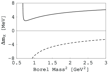
Figure 2: The mass difference of the $K$ meson, as a function of the Borel mass square $M_{B}^{2}$. The dashed curve is obtained when $s_{0}(K^{0},\bar{K}^{0})=s_{0}(K^{\pm})=0.900$ GeV². The solid curve is obtained when $s_{0}(K^{0},\bar{K}^{0})=0.916$ GeV² and $s_{0}(K^{\pm})=0.900$ GeV².

Now let us study the $K$ decay constant. We need to input the mass of the $K$ meson which we use the experimental values, $m_{K^{0}(\bar{K}^{0})}=497.6$ MeV and $m_{K^{\pm}}=493.7$ MeV Eidelman:2004wy . The left panel of Fig. 3 shows the $K^{\pm}$ decay constant $f_{K^{\pm}}$ as a function of the Borel mass square $M_{B}^{2}$ when $s_{0}=0.900$ GeV² is used. The result for $K^{0}$ ($\bar{K}^{0}$) and $K^{\pm}$ can not be distinguished in this figure (see the right panel and discussion below). It is interesting that the sum rule values take around $165$ MeV with a good Borel stability and is consistent with the experimental value $f_{K^{\pm}}=159.8\pm 1.84$ MeV Eidelman:2004wy .

The difference of the $K$ decay constants $\Delta f_{K}=f_{K^{0}(\bar{K}^{0})}-f_{K^{\pm}}$ is plotted in the right panel of Fig. 3, as a function of the Borel mass square $M_{B}^{2}$. The meaning of the dashed and solid curves are the same as for Fig. 2. When the same threshold values are used, $\Delta f_{K}$ takes values $0.2\sim 0.5$ MeV for $1\lesssim M_{B}^{2}\lesssim 3$ GeV² with some strong Borel mass dependence. However, when using the different threshold values, we obtain $\Delta f_{K}=1.5\pm 0.2$ MeV with a good Borel stability for $1\lesssim M_{B}^{2}\lesssim 3$ GeV².

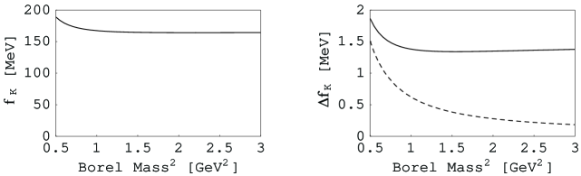
Figure 3: The left panel shows the $K^{\pm}$ decay constant $f_{K^{\pm}}$, as a function of the Borel mass square $M_{B}^{2}$, for threshold value $s_{0}=0.900$ GeV². The right panel shows the difference of the $K$ decay constants, as a function of the Borel mass square $M_{B}^{2}$. The dashed curve is obtained when $s_{0}(K^{0},\bar{K}^{0})=s_{0}(K^{\pm})=0.900$ GeV². The solid curve is obtained when $s_{0}(K^{0},\bar{K}^{0})=0.916$ GeV² and $s_{0}(K^{\pm})=0.900$ GeV².

III.2 The QCD Sum Rule for the $K^{*}$ Meson

For the $K^{*}$ meson, we expect that the QCD sum rule works well just as in the case of the $\rho$ meson. In order to check the validity of the present sum rule, we show the mass of $K^{*\pm}$ in the left panel of Fig. 4, where we find a very good Borel stability. The absolute value depends slightly on the choice of the threshold value $s_{0}$, which we choose $s_{0}=1.80$ GeV² to reproduce the experimental value $m_{K^{*\pm}}=891.7$ MeV Eidelman:2004wy . The result for $K^{*0}$ ($\bar{K}^{*0}$) is very similar.

The mass difference $\Delta m_{K^{*}}=m_{K^{*0}}-m_{K^{*\pm}}$ is shown in the right panel of Fig. 4 as a function of the Borel mass square $M_{B}^{2}$. The dashed curve is obtained when the same threshold value $s_{0}=1.80$ GeV² is used both for $K^{*0}$ ($\bar{K}^{*0}$) and $K^{*\pm}$. The Borel stability is not good. We can fine tune the threshold value $s_{0}$ again and use different ones for $K^{*0}$ ($\bar{K}^{*0}$) and $K^{*\pm}$. The solid line is obtained when we take $s_{0}(K^{*0},\bar{K}^{*0})=1.83$ GeV² and $s_{0}(K^{*\pm})=1.80$ GeV², with which the sum rule value takes $\Delta m_{K^{*}}=7\pm 1$ MeV ($M_{B}^{2}\gtrsim 1$ GeV²). This is consistent with the experimental value $\Delta m_{K^{*}}=6.7\pm 1.2$ MeV Eidelman:2004wy . The Borel stability is much improved for $M_{B}^{2}\gtrsim 1$ GeV².

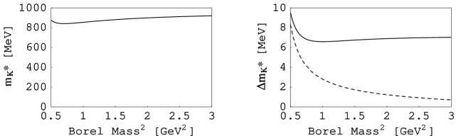
Figure 4: The masses of $K^{*0}$($\bar{K}^{*0}$) and $K^{*\pm}$ and their differences, as a function of the Borel mass square $M_{B}^{2}$ for threshold values $s_{K^{*0},\bar{K}^{*0}}=1.83$ GeV² and $s_{K^{*\pm}}=1.80$ GeV².

For the study of $K^{*}$ decay constant, we use the experimental values for the mass of $K^{*}$ meson, $m_{K^{*0}}=896.1$ MeV and $m_{K^{*\pm}}=891.7$ MeV Eidelman:2004wy . The left panel of Fig. 5 shows the $K^{*\pm}$ decay constant $f_{K^{*\pm}}$ as a function of the Borel mass square $M_{B}^{2}$ when $s_{0}=1.80$ GeV² is used. The result for $K^{*0}$ ($\bar{K}^{*0}$) is very similar. The sum rule values take around $230$ MeV with a good Borel stability. We can estimate the decay rate of $\tau^{-}\rightarrow K^{*-}\nu_{\tau}$ as Donoghue:1992

$$\Gamma_{\tau\rightarrow K^{*-}\nu_{\tau}} = |V_{us}|^{2}{G_{\mu}^{2}\over 8\pi}\left(f_{K^{*}}\over\sqrt{2}m_{K^{*}}\right)^{2}m^{3}_{\tau}m^{2}_{K^{*}}\left(1-{m^{2}_{K^{*}}\over m^{2}_{\tau}}\right)^{2}\left(1+2{m^{2}_{K^{*}}\over m^{2}_{\tau}}\right)$$

$$= 3.42\times 10^{-14}\mbox{ GeV}\,,$$

which is not far from the experimental values $\Gamma_{\tau^{-}\rightarrow K^{*-}\nu_{\tau}}=2.78\times 10^{-14}$ GeV Eidelman:2004wy .

We can also calculate the decay rate of $\tau^{-}\rightarrow K^{-}\nu_{\tau}$

$$\Gamma_{\tau\rightarrow K^{-}\nu_{\tau}} = |V_{us}|^{2}{G_{\mu}^{2}\over 8\pi}\left(f_{K}\over\sqrt{2}m_{K}\right)^{2}m^{3}_{\tau}m^{2}_{K}\left(1-{m^{2}_{K}\over m^{2}_{\tau}}\right)^{2}$$

$$= 1.67\times 10^{-14}\mbox{ GeV}\,,$$

which is also consistent with the experimental values $\Gamma_{\tau^{-}\rightarrow K^{-}\nu_{\tau}}=1.48\times 10^{-14}$ GeV Eidelman:2004wy .

The difference of the $K^{*}$ decay constants $\Delta f_{K^{*}}=f_{K^{*0}(\bar{K}^{*0})}-f_{K^{*\pm}}$ is plotted in the right panel of Fig. 5, as a function of the Borel mass square $M_{B}^{2}$. The meaning of the dashed and solid curves are the same as for Fig. 4.

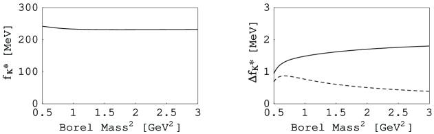
Figure 5: The decay constants of $K^{*0}$($\bar{K}^{*0}$) and $K^{*\pm}$ and their differences, as a function of the Borel mass square $M_{B}^{2}$ for threshold values $s_{K^{*0},\bar{K}^{*0}}=1.83$ GeV² and $s_{K^{*\pm}}=1.80$ GeV².

III.3 The Threshold Value $s_{0}$ Dependence

Finally, let us investigate $s_{0}$ dependence of the present QCD sum rule analyses. In order to see its typical behavior, we fix the Borel mass to be $M_{B}^{2}=1$ GeV². We use the two threshold values

$$s_{0}(K^{0},K^{*0}) = s_{0}+\Delta s_{0},\mbox{ ~{}~{}~{}~{}~{}for $K^{0}$ or $K^{*0}$}\,,$$

$$s_{0}(K^{\pm},K^{*\pm}) = s_{0},\mbox{ ~{}~{}~{}~{}~{}~{}~{}~{}~{}~{}~{}~{}~{}~{}for $K^{\pm}$ or $K^{*\pm}$}\,.$$

As $s_{0}$ is varied, $\Delta s_{0}$ is fixed such that the experimental mass difference $\Delta m_{K}$ or $\Delta m_{K^{*}}$ is reproduced. The differences of the decay constants $\Delta f$ are then computed as functions of $s_{0}$. The resulting $\Delta s_{0}$ and $\Delta f$ are plotted in Fig. 6 for $K$ and in Fig. 7 for $K^{*}$. It is interesting to observe that although $\Delta s_{0}$ are monotonically increasing functions, $\Delta f$’s are rather stable as $s_{0}$ is varied. It would be an indication that the present sum rule analyses especially for $\Delta f$ are stable.

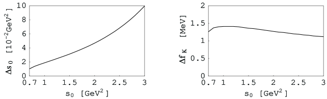
Figure 6: $\Delta s_{0}\equiv s_{0}(K^{0})-s_{0}(K^{\pm})$ and $\Delta f_{K}$ as functions of $s_{0}$. $\Delta s_{0}$ is determined so as to reproduce the experimental value of $\Delta m_{K}=3.972$ MeV at $M_{B}^{2}=1$ GeV².

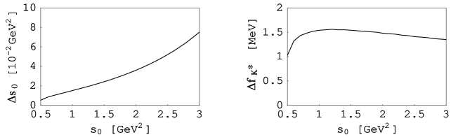
Figure 7: $\Delta s_{0}\equiv s_{0}(K^{*0})-s_{0}(K^{*\pm})$ and $\Delta f_{K^{*}}$ as functions of $s_{0}$. $\Delta s_{0}$ is determined so as to reproduce the experimental value of $\Delta m_{K^{*}}=6.7$ MeV at $M_{B}^{2}=1$ GeV².

IV Summary

In this paper, we have studied isospin breaking for masses and decay constants of $K$ and $K^{*}$. We have adopted gauge invariant currents coupled by a photon field. We have then estimated isospin symmetry breaking effects through different values of the parameters such as quark masses, condensates and threshold values. Quark masses and condensates were fixed from other sources, while the threshold values were fixed such that the mass differences of charged and neutral $K$ and $K^{*}$ were reproduced. The resulting decay constants were found to be very stable against the change in the Borel mass and the threshold values. The resulting values for $\Delta m$ and $\Delta f$ are consistent with experimental values.

The present analysis with good stability indicates that the QCD sum rule can be applied to study the symmetry breaking effects in hadron physics. In the near future, BESIII collaboration will measure the mass splittings of $K$ and $K^{\ast}$ systems precisely. Investigation of isospin symmetry breaking patterns helps to explore the low-energy sector of the underlying QCD dynamics.

References

(1)
T. Das, G. S. Guralnik, V. S. Mathur, F. E. Low and J. E. Young,
Phys. Rev. Lett. 18, 759 (1967).
(2)
K. Fujikawa and P. J. O’Donnell,
Phys. Rev. D 9, 461 (1974).
(3)
L. Scorzato,
Eur. Phys. J. C 37, 445 (2004)
[arXiv:hep-lat/0407023].
(4)
W. A. Bardeen, J. Bijnens and J. M. Gerard,
Phys. Rev. Lett. 62, 1343 (1989).
(5)
A. Duncan, E. Eichten and H. Thacker,
Phys. Rev. Lett. 76, 3894 (1996)
[arXiv:hep-lat/9602005].
(6)
S. L. Zhu and Z. P. Li,
Phys. Rev. D 55, 7093 (1997)
[arXiv:hep-ph/9703371].
(7)
L. S. Kisslinger and Z. P. Li,
Phys. Rev. Lett. 74, 2168 (1995)
[arXiv:hep-ph/9409377].
(8)
M. A. Shifman, A. I. Vainshtein and V. I. Zakharov,
Nucl. Phys. B 147, 385 (1979).
(9)
P. Ball and R. Zwicky,
Phys. Lett. B 633, 289 (2006)
[arXiv:hep-ph/0510338].
(10)
L. J. Reinders, H. Rubinstein and S. Yazaki,
Phys. Rept. 127, 1 (1985).
(11)
J. Gasser and H. Leutwyler,
Nucl. Phys. B 250, 465 (1985).
(12)
T. Hatsuda, H. Hogaasen and M. Prakash,
Phys. Rev. C 42, 2212 (1990).
(13)
V. L. Chernyak and A. R. Zhitnitsky,
Phys. Rept. 112, 173 (1984).
(14)
S. Eidelman et al. [Particle Data Group],
Phys. Lett. B 592 (2004) 1.
(15)
K. C. Yang, W. Y. P. Hwang, E. M. Henley and L. S. Kisslinger,
Phys. Rev. D 47, 3001 (1993).
(16)
V. Gimenez, V. Lubicz, F. Mescia, V. Porretti and J. Reyes,
Eur. Phys. J. C 41, 535 (2005)
[arXiv:hep-lat/0503001].
(17)
M. Jamin,
Phys. Lett. B 538, 71 (2002)
[arXiv:hep-ph/0201174].
(18)
B. L. Ioffe and K. N. Zyablyuk,
Eur. Phys. J. C 27, 229 (2003)
[arXiv:hep-ph/0207183].
(19)
A. A. Ovchinnikov and A. A. Pivovarov,
Sov. J. Nucl. Phys. 48, 721 (1988)
[Yad. Fiz. 48, 1135 (1988)].
(20)
J. F. Donoghue, E. Golowich and B. R. Holstein,
Dynamics of the Standard Model (Cambridge University Press, 1992)