Energy density of the Glasma

Abstract

The initial energy density produced in an ultrarelativistic heavy ion collision can, in the color glass condensate framework, be factorized into a product of the integrated gluon distributions of the nuclei. Although this energy density is well defined without any infrared cutoff besides the saturation scale, it is apparently logarithmically ultraviolet divergent. We argue that this divergence is not physically meaningful and does not affect the behavior of the system at any finite proper time.

I Introduction

The matter produced at central rapidities in a heavy ion collision is dominated by the small $x$ partons in the wave function of the high energy nuclei. These degrees of freedom can, because of their high occupation numbers, be described as a classical Weizsäcker-Williams color field. The source for this field is formed by the large $x$ partons, which are seen by the small $x$ ones as classical color charges. The nonlinear interactions between the small $x$ gluons give rise to gluon saturation, and the wavefunction is described by an energy (or $x$) dependent saturation scale. This way of understanding the small $x$ wavefunction is known as the color glass condensate. A model incorporating these physical features was written down by McLerran and Venugopalan (MV) McLerran:1994ni ; McLerran:1994ka ; McLerran:1994vd .

The initial transverse energy and gluon multiplicity in a collision of two sheets of color glass in the MV model has been calculated to all orders in the gluon field already some time ago Krasnitz:1998ns ; Krasnitz:1999wc ; Krasnitz:2000gz ; Krasnitz:2001qu ; Lappi:2003bi ; Lappi:2004sf . Recently there has been a renewed interest in the very early time behavior of these classical “Glasma” gluon fields Lappi:2006fp ; Fries:2006pv , in the context of pair production from the classical background field Gelis:2003vh ; Gelis:2004jp ; Lappi:2006nx ; Gelis:2005pb ; Fujii:2005rm ; Fujii:2005vj ; Kharzeev:2005iz ; Kharzeev:2006zm and parity violation through the Chern-Simons charge density of the fields Kharzeev:2001ev ; Kharzeev:2004ey . More attention has also been paid to the 3-dimensional energy density (instead of the energy per unit rapidity) of these field configurations as a quantity that could be directly related to the initial conditions of hydrodynamical calculations Hirano:2004rs ; Hirano:2004rsb .

The purpose of this note is to clarify some properties of the initial energy density of the gauge fields in the MV model. We shall first, in Sec. II, demonstrate that the initial energy density can be completely factorized into the product of the gluon distribution functions of the colliding nuclei. Going to finite proper times, or looking at the multiplicity, will change this factorization into a convolution of the unintegrated gluon distributions. We shall then, in Sec. III, go on to discuss the known properties of the correlator of two pure gauge fields involved in the initial energy density and, in Sec. IV, try to understand the behavior of large ${\mathbf{p}_{T}}$ modes with the help of the lowest order perturbative solution of the classical field equations.

II Initial condition

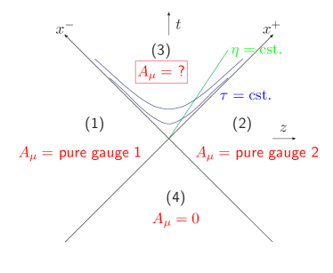
Figure 1: The color fields in different regions of spacetime. In regions (1) and (2), where only one of the nuclei has passed by, the field is the pure gauge field of this one nucleus. Inside region (3) the field is known numerically, but the initial condition for the field on the light cone $\tau=0$ is determined by the two pure gauge fields.

Figure 2: Components of the color field, computed on a $512^{2}$ lattice with $g^{2}\mu R_{A}=67.7$.

Because of their high speed and Lorentz time dilation, the large $x$ degrees of freedom are seen by the low $x$ fields as slowly evolving in light cone time. They form classical, static (in light cone time) sources on the light cones:

$$J^{\mu}=\delta^{\mu+}\rho_{(1)}(\mathbf{x}_{T},x^{-})+\delta^{\mu-}\rho_{(2)}(\mathbf{x}_{T},x^{+}),$$ (1)

where the support of the sources around the light cone must be understood as being very close to a delta function: $\rho_{(1,2)}(\mathbf{x}_{T},x^{\pm})\sim\delta(x^{\pm})$. We shall work here in the Schwinger gauge $A_{\tau}=\left(x^{+}A^{-}+x^{-}A^{+}\right)/\tau=0$, in which the current (1) is not rotated by the soft classical field; in more general gauges Eq. (1) should be dressed by Wilson lines to maintain its covariant conservation. The Weizsäcker-Williams fields describing the softer degrees of freedom can then be computed from the classical Yang-Mills equation

$$[D_{\mu},F^{\mu\nu}]=J^{\nu}.$$ (2)

In the light cone gauge the field of one nucleus is a pure gauge outside the light cone (see Fig. 1)

$$A^{i}_{(1,2)}(\mathbf{x}_{T})=\frac{i}{g}U_{(1,2)}(\mathbf{x}_{T})\partial_{i}U^{\dagger}_{(1,2)}(\mathbf{x}_{T}),$$ (3)

where the SU(3) matrices $U_{(m)}(\mathbf{x}_{T})$ are determined from the color sources as

$$U_{(1,2)}(\mathbf{x}_{T})=P\exp\left\{-ig\int\,\mathrm{d}x^{\pm}\frac{1}{\boldsymbol{\nabla}_{T}^{2}}\rho_{(1,2)}(\mathbf{x}_{T},x^{\pm})\right\}.$$ (4)

In the original MV model, which we shall be using here, the color charge densities are stochastic Gaussian random variables on the transverse plane: $\rho^{a}_{(1)}(\mathbf{x}_{T},x^{-})=\delta(x^{-})\rho^{a}(\mathbf{x}_{T})$ with

$$\langle\rho^{a}(\mathbf{x}_{T})\rho^{b}(\mathbf{y}_{T})\rangle=g^{2}\mu^{2}\delta^{ab}\delta^{2}(\mathbf{x}_{T}-\mathbf{y}_{T}),$$ (5)

where the density of color charges $g^{2}\mu$ is, up to a numerical constant and a logarithmic uncertainty, related to the saturation scale $Q_{\mathrm{s}}$.

The initial conditions for the fields in the future light cone between the two colliding sheets were derived and the equations of motion solved to lowest order in the fields in Kovner:1995ja ; Kovner:1995ts ; Gyulassy:1997vt (see also Ref. Kovchegov:1997ke for the same calculation in covariant gauge and Ref. Fries:2006pv for another formulation.) This initial condition has a simple expression in terms of the pure gauge fields of the two colliding nuclei (3):

$$A^{i} = A^{i}_{(1)}+A^{i}_{(1)}$$ (6)

$$A^{\eta} = \frac{ig}{2}\left[A^{i}_{(1)},A^{i}_{(2)}\right]$$ (7)

$$\partial_{\tau}A_{i} = 0$$ (8)

$$\partial_{\tau}A^{\eta} = 0.$$ (9)

Note that the metric in the $(\tau,\eta,\mathbf{x}_{T})$ coordinate system is $g_{\mu\nu}=\mathrm{diag}(1,-\tau^{2},-1,-1)$ so that $A_{\eta}=-\tau^{2}A^{\eta}$. In the Schwinger gauge $A^{\tau}=0$ the $\pm$ components of the gauge field are related by $A^{\pm}=\pm x^{\pm}A^{\eta}$. Because of the explicit time dependence in the metric $A^{\eta}$ corresponds, at $\tau=0$, to the $z$-component of the chromoelectric field. At the initial time the only nonzero components of the field strength tensor are the longitudinal electric and magnetic fields and consequently the energy density is given by

$$\varepsilon(\tau=0)=\lim_{\tau\to 0^{+}}\frac{1}{\tau}\frac{\,\mathrm{d}E}{\,\mathrm{d}^{2}\mathbf{x}_{T}\,\mathrm{d}\eta}=\\ \frac{1}{2}\,\mathrm{Tr}\,F_{ij}F_{ij}+4\,\mathrm{Tr}\,\left(A^{\eta}\right)^{2}.$$ (10)

Let us introduce a shorter notation for the correlation function of the pure gauge field of the nucleus when averaged with the distribution (5). We shall define the correlation function $G({\mathbf{p}_{T}})$ by

$$\left\langle A_{i}^{(m)a}({\mathbf{p}_{T}})A_{j}^{(n)b}({\mathbf{q}_{T}})\right\rangle\equiv\\ (2\pi)^{2}\delta^{mn}\delta^{ab}\delta^{2}({\mathbf{p}_{T}}+{\mathbf{q}_{T}})\frac{p_{i}p_{j}}{{\mathbf{p}_{T}}^{2}}G({\mathbf{p}_{T}}).$$ (11)

The index in parentheses $(m)$ refers to the two colliding nuclei, which are, naturally, independent of each other, thus the $\delta^{mn}$ in the correlator. The correlator must also be diagonal in the color index ($\delta^{ab}$) because there is no preferred direction in color space present in the problem. We are assuming translational invariance on the transverse plane ($\delta^{2}({\mathbf{p}_{T}}+{\mathbf{q}_{T}})$), which is justified because we are only interested in momentum scales much larger than the nuclear geometry effects which break this invariance (meaning that we are assuming $|{\mathbf{p}_{T}}|\gg 1/R_{A}$). The transverse spatial index structure $p_{i}p_{j}$ is the only one consistent with rotational invariance on the transverse plane (again, at momentum scales $|{\mathbf{p}_{T}}|\gg 1/R_{A}$ there is no preferred direction in the system to break this invariance).

Using the notation of Eq.  (11) the two terms in the energy density (10) become

$$\int\,\mathrm{d}^{2}\mathbf{x}_{T}\frac{1}{2}\,\mathrm{Tr}\,F_{ij}F_{ij} = \frac{1}{2}g^{2}{N_{\mathrm{c}}}\left({N_{\mathrm{c}}}^{2}-1\right)\pi R_{A}^{2}\int\frac{\,\mathrm{d}^{2}{\mathbf{k}_{T}}}{(2\pi)^{2}}\frac{\,\mathrm{d}^{2}{\mathbf{p}_{T}}}{(2\pi)^{2}}\left[{\mathbf{p}_{T}}^{2}{\mathbf{k}_{T}}^{2}-({\mathbf{p}_{T}}\cdot{\mathbf{k}_{T}})^{2}\right]\frac{G({\mathbf{p}_{T}})}{{\mathbf{p}_{T}}^{2}}\frac{G({\mathbf{k}_{T}})}{{\mathbf{k}_{T}}^{2}}$$ (12)

$$\int\,\mathrm{d}^{2}\mathbf{x}_{T}4\,\mathrm{Tr}\,\left(A^{\eta}\right)^{2} = \frac{1}{2}g^{2}{N_{\mathrm{c}}}\left({N_{\mathrm{c}}}^{2}-1\right)\pi R_{A}^{2}\int\frac{\,\mathrm{d}^{2}{\mathbf{k}_{T}}}{(2\pi)^{2}}\frac{\,\mathrm{d}^{2}{\mathbf{p}_{T}}}{(2\pi)^{2}}\left[({\mathbf{p}_{T}}\cdot{\mathbf{k}_{T}})^{2}\right]\frac{G({\mathbf{p}_{T}})}{{\mathbf{p}_{T}}^{2}}\frac{G({\mathbf{k}_{T}})}{{\mathbf{k}_{T}}^{2}}$$ (13)

and the final result factorizes into

$$\varepsilon|_{\tau=0}=\frac{g^{2}}{2}{N_{\mathrm{c}}}\left({N_{\mathrm{c}}}^{2}-1\right)\left[\int\frac{\,\mathrm{d}^{2}{\mathbf{p}_{T}}}{(2\pi)^{2}}G({\mathbf{p}_{T}})\right]^{2}.$$ (14)

Equation (14) is our main result. The initial energy density factorizes completely into a product of two terms, both of which only depend on the properties of one single nucleus. This happens only strictly at $\tau=0$.

Note that due to rotational invariance the initial energy density in the magnetic field, Eq. (12) and the electric field, Eq. (13) are equal. The discretized version of the computation on a transverse lattice breaks this rotational invariance (for an explicit expression see the lattice perturbation theory result in Appendix B of Ref. Krasnitz:1998ns ). This violation is largest for the momentum modes near the edges of the Brillouin zone. As we shall discuss in the following, for larger proper times these modes do not affect the energy density any more, and the energy densities in the longitudinal electric and magnetic fields approach each other, as can be seen in Fig. 2.

III Properties of the gauge field correlator

Let us then recall some known properties of $G({\mathbf{p}_{T}})$, the correlation function of the pure gauge fields defined in Eq. (11). In light cone quantization it is related to the unintegrated gluon distribution function

$$xG(x,Q^{2})=R_{A}^{2}\left({N_{\mathrm{c}}}^{2}-1\right)\int^{Q^{2}}\frac{\,\mathrm{d}^{2}{\mathbf{k}_{T}}}{(2\pi)^{2}}G({\mathbf{k}_{T}}).$$ (15)

Note, however, that our $G({\mathbf{p}_{T}})$ is equivalent to the unintegrated gluon distribution used to compute gluon production in pA-collisions only in the weak field limit. We refer the reader to Refs. Kharzeev:2003wz ; Blaizot:2004wu ; Gelis:2006tb for a discussion of the difference. Our $G({\mathbf{p}_{T}})$ is equivalent, up to the normalization, to $\phi^{\textrm{WW}}$ of Ref. Kharzeev:2003wz .

The correlator $G({\mathbf{p}_{T}})$ has been analytically evaluated in several papers Jalilian-Marian:1997xn ; Kovchegov:1996ty ; Kovchegov:1997pc . The result is expressed in closed form in coordinate space as

$$G(\mathbf{x}_{T})=\frac{4}{g^{2}{N_{\mathrm{c}}}\mathbf{x}_{T}^{2}}\left(1-e^{-\frac{{N_{\mathrm{c}}}}{8\pi}\mathbf{x}_{T}^{2}(g^{2}\mu)^{2}\ln\frac{1}{\Lambda|\mathbf{x}_{T}|}}\right).$$ (16)

Here $\Lambda$ is an infrared cutoff that one must introduce in order to invert the 2 dimensional Laplace operator. The same function can also be measured in the numerical setup used to compute the glasma fields Krasnitz:1998ns ; Krasnitz:1999wc ; Krasnitz:2000gz ; Krasnitz:2001qu ; Lappi:2003bi . The numerical procedure used is not exactly equivalent to the calculation leading to Eq. (16), because the source in Eq. (4) is taken as exactly a delta function on the light cone and the infrared divergence in inverting the Laplace operator $\boldsymbol{\nabla}_{T}^{2}$ is effectively regulated by the size of the lattice. These differences can, however, be absorbed into the infrared cutoff $\Lambda$, and the numerical evaluation (see in particular Fig. 3 of Ref. Krasnitz:2002mn ) of the correlator agrees with the behavior of Eq. (16). Note that to derive the correct initial conditions, Eqs. (3), (4), (6) and (7), it is essential to consider the source as spread out in the longitudinal coordinate. Only when this is done can one, in practice, take the source as a delta function on the light cone when evaluating the Wilson line, Eq. (4).

Let us then estimate the behavior of the correlator $G({\mathbf{p}_{T}})$ in momentum space. For small momenta $G({\mathbf{p}_{T}})$ diverges, but the divergence is only logarithmic and thus integrable. This is the essential feature of gluon saturation; bulk quantities that are sensitive to the harder modes in the spectrum, such as the energy density, are infrared finite when the nonlinear interactions are taken into account fully.

For large momenta $G({\mathbf{p}_{T}})$ has a perturbative tail behaving as $1/{\mathbf{p}_{T}}^{2}$, meaning that the integral $\int\,\mathrm{d}^{2}{\mathbf{p}_{T}}G({\mathbf{p}_{T}})$ and thus the initial energy density are seemingly ultraviolet divergent. This can be seen equivalently as the logarithmic ultraviolet divergence in Eq. (16),

$$\int\frac{\,\mathrm{d}^{2}{\mathbf{p}_{T}}}{(2\pi)^{2}}G({\mathbf{p}_{T}})=\lim_{|\mathbf{x}_{T}|\to 0}G(\mathbf{x}_{T})\\ =\frac{1}{2\pi g^{2}}(g^{2}\mu)^{2}\lim_{|\mathbf{x}_{T}|\to 0}\ln\frac{1}{|\mathbf{x}_{T}|\Lambda}.$$ (17)

We must emphasize that although Eq. (17) involves, for dimensional reasons, the infrared cutoff $\Lambda$, it corresponds to a divergence from large transverse momentum, or small distance, modes.

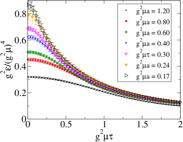
Figure 3: The energy density for different lattice spacings with $g^{2}\mu R_{A}=67.7$ The continuum limit corresponds to $g^{\mu}a\to 0$. The fields configurations have been calculated on transverse lattices of $100^{2}$ to $700^{2}$ points. The errors are statistical from between 20 configurations for the smaller lattices to 5 configurations on the largest ones.

The initial energy density of the glasma is infrared finite, but seemingly logarithmically ultraviolet divergent. There are two reasons why this divergence is fundamentally not a problem for the physical picture of the glasma. The first reason is that, as can be seen from Eq. (15), the divergence corresponds to large $Q^{2}$ and thus, for a fixed energy, large $x$ modes in the wavefunction. These are degrees of freedom that were, by our initial assumptions, not meant to be included in the classical field in the first place. It would therefore be physically well motivated to regulate them with an ultraviolet cutoff $\Lambda_{\mathrm{UV}}\gtrsim Q_{\mathrm{s}}$, and then match this cutoff with whatever way one treats these hard collisions. This is indeed the approach advocated e.g. in Ref. Fries:2006pv . The other reason for not worrying about the ultraviolet divergence is that, as we shall argue in the following, the energy density of the system at later proper times $\tau\sim 1/Q_{\mathrm{s}}$ has a finite $\Lambda_{\mathrm{UV}}\to\infty$ limit. Thus if one regulates the ultraviolet divergence in any convenient way and proceeds to solve the equations forward in time, the cutoff no longer significantly influences the later time evolution of the glasma fields.

IV Perturbative comparison and the apparent UV divergence

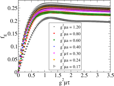
Figure 4: The energy per unit rapidity $f_{E}\equiv\frac{g^{2}}{\pi R_{A}^{2}(g^{2}\mu)^{3}}\frac{\,\mathrm{d}E}{\,\mathrm{d}\eta}$ (energy density divided by proper time) for different lattice spacings. The data are from the same numerical calculation as Fig. 3.

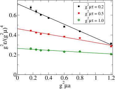
Figure 5: The energy density at proper times $\tau$ of 0.2, 0.5 and 1.0 in units of $1/g^{2}\mu$ as a function of the lattice spacing $a$, also in units of $1/g^{2}\mu$. The data are from the same calculation as Fig. 3. One sees that the energy density converges to the continuum limit ($g^{2}\mu a\to 0$) better at later times. The straight lines are linear extrapolations.

In the perturbative (lowest order in the source charge densities) solution Kovner:1995ja ; Kovner:1995ts ; Gyulassy:1997vt ; Kovchegov:1997ke the field amplitudes behave, in the two dimensional Coulomb gauge, like Bessel functions

$$A_{i}(\tau,{\mathbf{k}_{T}}) = A_{i}(\tau=0,{\mathbf{k}_{T}})J_{0}(|{\mathbf{k}_{T}}|\tau)$$ (18)

$$A_{\eta}(\tau,{\mathbf{k}_{T}}) = \frac{2\tau}{|{\mathbf{k}_{T}}|}A^{\eta}(\tau=0,{\mathbf{k}_{T}})J_{1}(|{\mathbf{k}_{T}}|\tau).$$ (19)

The energy density corresponding to this perturbative solution (this time dependence is also derived in Refs. Kovchegov:2005ss ; Kovchegov:2005kn ) is

$$\varepsilon=\frac{1}{2}g^{2}{N_{\mathrm{c}}}\left({N_{\mathrm{c}}}^{2}-1\right)\int\frac{\,\mathrm{d}^{2}{\mathbf{k}_{T}}}{(2\pi)^{2}}\frac{\,\mathrm{d}^{2}{\mathbf{p}_{T}}}{(2\pi)^{2}}G({\mathbf{p}_{T}})G({\mathbf{k}_{T}})\\ \times\left[J^{2}_{0}(|{\mathbf{p}_{T}}+{\mathbf{k}_{T}}|\tau)+J^{2}_{1}(|{\mathbf{p}_{T}}+{\mathbf{k}_{T}}|\tau)\right].$$ (20)

To lowest order in the sources the pure gauge field correlator is

$$G({\mathbf{p}_{T}})=\frac{1}{g^{2}}\frac{(g^{2}\mu)^{2}}{{\mathbf{p}_{T}}^{2}}$$ (21)

and, using the asymptotic behavior of the Bessel functions in Eq. (20), the energy density for large times reduces to

$$\varepsilon(\tau\to\infty)=\frac{1}{\tau}\int\,\mathrm{d}^{2}{\mathbf{k}_{T}}\frac{\,\mathrm{d}N}{\,\mathrm{d}y\,\mathrm{d}^{2}{\mathbf{k}_{T}}}|{\mathbf{k}_{T}}|$$ (22)

with the Bertsch-Gunion Gunion:1981qs type multiplicity resulting from the lowest order solution Kovner:1995ja ; Kovner:1995ts ; Gyulassy:1997vt ; Kovchegov:1997ke :

$$\frac{\,\mathrm{d}N}{\,\mathrm{d}y\,\mathrm{d}^{2}{\mathbf{k}_{T}}}=\frac{\pi R_{A}^{2}}{(2\pi)^{2}}\frac{{N_{\mathrm{c}}}({N_{\mathrm{c}}}^{2}-1)g^{6}\mu^{4}}{{\mathbf{k}_{T}}^{2}}\frac{1}{\pi}\\ \times\int\frac{\,\mathrm{d}^{2}{\mathbf{p}_{T}}}{(2\pi)^{2}}\frac{1}{{\mathbf{p}_{T}}^{2}({\mathbf{k}_{T}}-{\mathbf{p}_{T}})^{2}}.$$ (23)

Also in the full nonperturbative solution the most ultraviolet modes behave in the same way Krasnitz:2001qu ; Lappi:2003bi ; Krasnitz:2003jw . Let us now assume that we have computed the initial energy density with some ultraviolet cutoff $\Lambda_{\mathrm{UV}}$ (such as the inverse lattice spacing in the numerical calculation). The initial energy density Eq. (14) depends on this cutoff as $\ln^{2}\Lambda_{\mathrm{UV}}$, as can be seen in the numerical result in Fig. 3. After a time $\tau\gtrsim 1/\Lambda_{\mathrm{UV}}$, however, the time dependence of the modes near the cutoff changes from the initial $A_{i}(\tau)=A_{i}(0)\left(1+\mathcal{O}(\tau^{2})\right)$ to the asymptotic regime $A_{i}\sim 1/|{\mathbf{k}_{T}}|\tau$ and the contribution of these modes to the total energy density is suppressed by an additional power of the momentum, making the energy density finite in the limit $\Lambda_{\mathrm{UV}}\to\infty$. After a time $\tau\gtrsim 1/\Lambda_{\mathrm{UV}}$, or $\tau\gtrsim a$ in the lattice computation, the energy density then converges to a value that is independent of the lattice spacing, as shown in Fig. 4. The larger the proper time that one is looking at, the better the convergence in the continuum limit is. Figure 5 shows the continuum extrapolations of the energy densities at $g^{2}\mu\tau=0.2$, $0.5$ and $1.0$.

By turning this argument around one can see that if one takes first the continuum limit ($\Lambda_{\mathrm{UV}}\to\infty$ or $a\to 0$) for a finite $\tau$, the continuum extrapolated energy density will behave as $\ln^{2}1/\tau$. Thus if the limits are taken in this order, the energy density is indeed finite for all $\tau>0$, but diverges logarithmically at $\tau=0$. Note that this divergence is so weak that the energy per unit rapidity ($\tau\varepsilon$) is still zero at $\tau=0$. Thus we se that the solution of the field equations is well defined as an initial value problem only in the presence of an ultraviolet cutoff in the transverse momenta, but for later times the system loses memory of this cutoff. Incidentally, because of this feature one can argue that introducing of a finite initial time (such as done in Refs. Romatschke:2005pm ; Romatschke:2006nk to avoid the singularity resulting from broken boost invariance of the field configurations) does not really add another physical parameter into the model.

V Energy density in physical units and conclusion

For concreteness let us finally try to express the results shown in Figs. 3, 4 and 5 in physical units. Due to the difficulty in fixing exactly the right value of the color charge density parameter $g^{2}\mu$ this is not necessarily straightforward. For RHIC energies one can argue, based on both the gluon multiplicity found in the numerical calculation Krasnitz:2000gz ; Krasnitz:2001qu ; Lappi:2003bi and counting the number of large $x$ degrees of sources in the wavefunction from conventional parton distribution functions Gyulassy:1997vt that the relevant value would be $g^{2}\mu=2\ \textrm{GeV}$. Other estimates, e.g. Gelis:2005pb , give a smaller value, so $g^{2}\mu=2\ \textrm{GeV}$ should be considered an upper bound for RHIC. For LHC energies the estimate based on parton distributions Gyulassy:1997vt gives $g^{2}\mu\sim 4\ \textrm{GeV}$, but this is most certainly an overestimate, since the calculation in Ref. Gyulassy:1997vt is based on parton distributions in the proton and does not take into account shadowing corrections. Another way of estimating the color charge density is based on the small $x$ scaling properties observed in deep inelastic scattering data Golec-Biernat:1998js ; Golec-Biernat:1999qd ; Stasto:2000er ; Freund:2002ux ; Kharzeev:2004if . The saturation scale in this scaling can then be related to the MV model color charge density Iancu:2003xm ; Weigert:2005us . This line of thought leads to a scaling $Q_{\mathrm{s}}^{2}\sim(g^{2}\mu)^{2}\sim\sqrt{s}^{\bar{\lambda}}$, where $\bar{\lambda}=\lambda/(1+\lambda/2)$ and a fit to the HERA data Golec-Biernat:1998js gives $\lambda=0.288$ and thus $\bar{\lambda}\approx 0.25$. The result for the color charge density at the LHC would be $g^{2}\mu\approx 3\ \textrm{GeV},$ which is the value we will use in the following.

As we have seen, the energy density strictly at $\tau=0$ is not the best quantity to look at. Let us instead estimate the energy density at the time $\tau=1/g^{2}\mu$. This is when, as can be seen from Fig. 4, the $1/\tau$–decrease of the energy density seems to start. The simple linear continuum extrapolation of Fig. 5 yields $\varepsilon(\tau=1/g^{2}\mu)=0.26(g^{2}\mu)^{4}/g^{2}$. Using $g=2$ we then get the estimates $\varepsilon(\tau=0.1\ \textrm{fm})\approx 130\ \textrm{GeV}/\!\ \textrm{fm}^{3}$ for RHIC and $\varepsilon(\tau=0.07\ \textrm{fm})\approx 700\ \textrm{GeV}/\!\!\ \textrm{fm}^{3}$ for the LHC. This estimate agrees with the values given in Ref. Krasnitz:2003jw for $\tau=3/g^{2}\mu$ when the $\sim 1/\tau$ behavior of the energy density is taken into account. The uncertainty due to the unprecise value of $g^{2}\mu$ in these numbers is quite large because of the power law dependence $\varepsilon\sim(g^{2}\mu)^{4}$.

In conclusion, we have shown that the initial 3 dimensional energy density of the Glasma fields in the MV model can be expressed as a product of of the (integrated) gluon distribution functions of the colliding nuclei. Only the energy density at later times and the multiplicity involve convolutions of the unintegrated gluon distributions, probing the ${\mathbf{k}_{T}}$-distributions in the wavefunctions of the colliding nuclei in more detail. We have recalled the known properties if the pure gauge field correlator Eq. (11) appearing in the initial energy density. As expected from general gluon saturation arguments, the initial energy density is infrared finite when the gluon fields are solved to all orders in the source. The energy density strictly at $\tau=0$ is, however, ultraviolet divergent in the MV model. We show, both by a direct numerical calculation and by examining the time dependence of the ultraviolet modes, that this divergence does not persist when the equations of motion are solved to times larger than the inverse ultraviolet cutoff.

- (1) L. D. McLerran and R. Venugopalan, Phys. Rev. D49, 2233 (1994), [arXiv:hep-ph/9309289].
- (2) L. D. McLerran and R. Venugopalan, Phys. Rev. D49, 3352 (1994), [arXiv:hep-ph/9311205].
- (3) L. D. McLerran and R. Venugopalan, Phys. Rev. D50, 2225 (1994), [arXiv:hep-ph/9402335].
- (4) A. Krasnitz and R. Venugopalan, Nucl. Phys. B557, 237 (1999), [arXiv:hep-ph/9809433].
- (5) A. Krasnitz and R. Venugopalan, Phys. Rev. Lett. 84, 4309 (2000), [arXiv:hep-ph/9909203].
- (6) A. Krasnitz and R. Venugopalan, Phys. Rev. Lett. 86, 1717 (2001), [arXiv:hep-ph/0007108].
- (7) A. Krasnitz, Y. Nara and R. Venugopalan, Phys. Rev. Lett. 87, 192302 (2001), [arXiv:hep-ph/0108092].
- (8) T. Lappi, Phys. Rev. C67, 054903 (2003), [arXiv:hep-ph/0303076].
- (9) T. Lappi, Phys. Rev. C70, 054905 (2004), [arXiv:hep-ph/0409328].
- (10) T. Lappi and L. McLerran, Nucl. Phys. A772, 200 (2006), [arXiv:hep-ph/0602189].
- (11) R. J. Fries, J. I. Kapusta and Y. Li, arXiv:nucl-th/0604054.
- (12) F. Gelis and R. Venugopalan, Phys. Rev. D69, 014019 (2004), [arXiv:hep-ph/0310090].
- (13) F. Gelis, K. Kajantie and T. Lappi, Phys. Rev. C71, 024904 (2005), [arXiv:hep-ph/0409058].
- (14) T. Lappi, arXiv:hep-ph/0606090.
- (15) F. Gelis, K. Kajantie and T. Lappi, Phys. Rev. Lett. 96, 032304 (2006), [arXiv:hep-ph/0508229].
- (16) H. Fujii, F. Gelis and R. Venugopalan, Eur. Phys. J. C43, 139 (2005), [arXiv:hep-ph/0502204].
- (17) H. Fujii, F. Gelis and R. Venugopalan, Phys. Rev. Lett. 95, 162002 (2005), [arXiv:hep-ph/0504047].
- (18) D. Kharzeev and K. Tuchin, Nucl. Phys. A753, 316 (2005), [arXiv:hep-ph/0501234].
- (19) D. Kharzeev, E. Levin and K. Tuchin, arXiv:hep-ph/0602063.
- (20) D. Kharzeev, A. Krasnitz and R. Venugopalan, Phys. Lett. B545, 298 (2002), [arXiv:hep-ph/0109253].
- (21) D. Kharzeev, Phys. Lett. B633, 260 (2006), [arXiv:hep-ph/0406125].
- (22) T. Hirano and Y. Nara, Nucl. Phys. A743, 305 (2004), [arXiv:nucl-th/0404039].
- (23) T. Hirano and Y. Nara, J. Phys. G30, S1139 (2004), [arXiv:nucl-th/0403029].
- (24) A. Kovner, L. D. McLerran and H. Weigert, Phys. Rev. D52, 6231 (1995), [arXiv:hep-ph/9502289].
- (25) A. Kovner, L. D. McLerran and H. Weigert, Phys. Rev. D52, 3809 (1995), [arXiv:hep-ph/9505320].
- (26) M. Gyulassy and L. D. McLerran, Phys. Rev. C56, 2219 (1997), [arXiv:nucl-th/9704034].
- (27) Y. V. Kovchegov and D. H. Rischke, Phys. Rev. C56, 1084 (1997), [arXiv:hep-ph/9704201].
- (28) E. Iancu, A. Leonidov and L. D. McLerran, Nucl. Phys. A692, 583 (2001), [arXiv:hep-ph/0011241].
- (29) D. Kharzeev, Y. V. Kovchegov and K. Tuchin, Phys. Rev. D68, 094013 (2003), [arXiv:hep-ph/0307037].
- (30) J. P. Blaizot, F. Gelis and R. Venugopalan, Nucl. Phys. A743, 13 (2004), [arXiv:hep-ph/0402256].
- (31) F. Gelis, A. M. Stasto and R. Venugopalan, arXiv:hep-ph/0605087.
- (32) J. Jalilian-Marian, A. Kovner, L. D. McLerran and H. Weigert, Phys. Rev. D55, 5414 (1997), [arXiv:hep-ph/9606337].
- (33) Y. V. Kovchegov, Phys. Rev. D54, 5463 (1996), [arXiv:hep-ph/9605446].
- (34) Y. V. Kovchegov, Phys. Rev. D55, 5445 (1997), [arXiv:hep-ph/9701229].
- (35) A. Krasnitz, Y. Nara and R. Venugopalan, Nucl. Phys. A717, 268 (2003), [arXiv:hep-ph/0209269].
- (36) Y. V. Kovchegov, Nucl. Phys. A762, 298 (2005), [arXiv:hep-ph/0503038].
- (37) Y. V. Kovchegov, Nucl. Phys. A764, 476 (2006), [arXiv:hep-ph/0507134].
- (38) J. F. Gunion and G. Bertsch, Phys. Rev. D25, 746 (1982).
- (39) A. Krasnitz, Y. Nara and R. Venugopalan, Nucl. Phys. A727, 427 (2003), [arXiv:hep-ph/0305112].
- (40) P. Romatschke and R. Venugopalan, Phys. Rev. Lett. 96, 062302 (2006), [arXiv:hep-ph/0510121].
- (41) P. Romatschke and R. Venugopalan, Phys. Rev. D74, 045011 (2006), [arXiv:hep-ph/0605045].
- (42) K. Golec-Biernat and M. Wusthoff, Phys. Rev. D59, 014017 (1999), [arXiv:hep-ph/9807513].
- (43) K. Golec-Biernat and M. Wusthoff, Phys. Rev. D60, 114023 (1999), [arXiv:hep-ph/9903358].
- (44) A. M. Stasto, K. Golec-Biernat and J. Kwiecinski, Phys. Rev. Lett. 86, 596 (2001), [arXiv:hep-ph/0007192].
- (45) A. Freund, K. Rummukainen, H. Weigert and A. Schafer, Phys. Rev. Lett. 90, 222002 (2003), [arXiv:hep-ph/0210139].
- (46) D. Kharzeev, E. Levin and M. Nardi, Nucl. Phys. A747, 609 (2005), [arXiv:hep-ph/0408050].
- (47) E. Iancu and R. Venugopalan, arXiv:hep-ph/0303204.
- (48) H. Weigert, Prog. Part. Nucl. Phys. 55, 461 (2005), [arXiv:hep-ph/0501087].