Global three-parameter model for neutrino oscillations using Lorentz violation

Abstract

A model of neutrino oscillations is presented that has only three degrees of freedom and is consistent with existing data. The model is a subset of the renormalizable sector of the Standard-Model Extension (SME), and it offers an alternative to the standard three-neutrino massive model. All classes of neutrino data are described, including solar, reactor, atmospheric, and LSND oscillations. The disappearance of solar neutrinos is obtained without matter-enhanced oscillations. Quantitative predictions are offered for the ongoing MiniBooNE experiment and for the future experiments OscSNS, NOvA, and T2K.

I Introduction

Local Lorentz invariance is a basic feature of our best existing theory, which is the Standard Model (SM) coupled to General Relativity (GR). This theory is widely believed to be the effective low-energy limit of an underlying structure that unifies quantum physics and gravity at the Planck scale, $M_{P}\simeq 10^{19}$ GeV. Direct experimentation at this scale is infeasible, but sensitive measurements might detect suppressed low-energy signals of the expected new physics, including small violations of Lorentz and CPT symmetry cpt04 ; reviews . At presently attainable energies, these unconventional effects can be characterized in the language of effective field theory kp . Extending the GR-coupled SM by adding all terms that involve operators for Lorentz violation and that are scalars under coordinate transformations results in a general effective field theory called the Standard-Model Extension (SME). The leading terms in this theory include those of the SM and GR, together with ones violating Lorentz and CPT symmetry constructed from SM and GR fields ck ; akgrav .

Neutrinos are natural quantum interferometers, and so neutrino oscillations represent sensitive phenomena with which to conduct searches for physics beyond the minimal SM, including Lorentz and CPT violation. Compelling experimental evidence for oscillations exists, and they are conventionally attributed to neutrino masses. In the standard three-neutrino massive model pdg , the effective hamiltonian for neutrino propagation and oscillation is a 3$\times$3 matrix determined by six parameters, consisting of two squared-mass differences $\Delta m^{2}_{\odot}$, $\Delta m^{2}_{\rm atm}$, three mixing angles $\theta_{12}$, $\theta_{23}$, $\theta_{13}$, and a phase $\delta$. This model can reproduce the observed features of the solar-neutrino suppression Homestake ; SAGE ; GNO ; Super-Ksol ; SNOsol , the atmospheric-neutrino oscillations MACRO ; K2K ; Super-Kosc ; MINOS , and the KamLAND results KamLANDosc . However, the model cannot reproduce the LSND signal LSND2 .

The presence of Lorentz and CPT violation in the underlying theory can produce additional or alternative sources of neutrino oscillations in the low-energy effective Lagrange density, which are contained in the neutrino sector of the SME. Even if attention is restricted to three generations of active neutrinos and dominant effects, the SME involves many terms and many types of effects km1 . These oscillation effects are controlled by coefficients for Lorentz violation forming various 3$\times$3 matrices denoted $(a_{L})^{\alpha}_{ab}$, $(c_{L})^{\alpha\beta}_{ab}$, etc., where $\alpha$, $\beta$ are Lorentz indices and the matrix indices $a$, $b$ label neutrino flavor and span $e$, $\mu$, $\tau$. It is elegant to regard these coefficients as arising from spontaneous Lorentz violation ksp , which is consistent with Riemann geometry akgrav and may be ubiquitous in effective field theories bak . Some of the neutrino coefficients for Lorentz violation act to mimic aspects of conventional mass-induced oscillations, while others predict qualitatively new features of oscillations such as sidereal variations, direction dependence, unconventional spectral behavior, Lorentz-violating seesaws, neutrino-antineutrino mixing, and more.

The LSND collaboration recently analyzed the sidereal-time dependence of their reported $\bar{\nu}_{e}$ appearance signal LVLSND , using the short-baseline approximation km3 . Since this signal cannot be incorporated within the standard three-neutrino massive model, a possible explanation is Lorentz violation. The scale required to generate a neutrino-oscillation signal at the LSND energies $E\simeq 10^{-2}$ GeV was found to be of order $10^{-19}$ GeV for $(a_{L})^{\alpha}_{e\mu}$ and $(c_{L})^{\alpha\beta}_{e\mu}E$. This result is compatible with the dimensionless ratio $\simeq 10^{-17}$ of electroweak to Planck scales that might be expected to control suppression of Planck-scale physics. The sensitivity achieved is comparable to other searches for Lorentz and CPT violation using interferometric techniques in high-energy physics involving $K$ oscillations KTeV , $D$ oscillations FOCUS , and $B_{d}$ oscillations BaBar ; BELLE ; OPAL ; DELPHI , including ones with sidereal variations ak . More generally, the SME sensitivities attainable with various types of neutrino searches can be comparable km1 to those achieved in the numerous experiments in astrophysics, atomic physics, optical physics, nuclear physics, and particle physics cpt04 ; reviews .

Each coefficient for Lorentz violation leads to an energy behavior different from that of a neutrino mass, so estimates for the size of possible Lorentz violation may be found by considering the energy dependence of the existing neutrino-oscillation data cg ; bpww ; bbm ; dgpg ; hmw . With this approach, profitable experiments for certain types of coefficients would involve ultra-high-energy neutrinos gghm because the long-baselines and high-energies involved would yield high sensitivity to certain small Lorentz-violating terms. However, it has been shown that some special combinations of coefficients for Lorentz violation can mimic a mass-like energy dependence through a Lorentz-violating seesaw mechanism, even if the hamiltonian contains no mass terms. The so-called ‘bicycle’ model km2 offers a simple example with only two coefficients for Lorentz violation. Despite having no neutrino mass in the hamiltonian, the model reproduces many features of the neutrino-oscillation data through a pseudomass term generated by a seesaw.

In this work, we describe a model for neutrino oscillations based on the SME that, like the bicycle model, uses one CPT-odd coefficient and one CPT-even coefficient. However, we also introduce a mass term, so the hamiltonian has three degrees of freedom. This ‘tandem’ model has two Lorentz-violating seesaw mechanisms that interplay in interesting ways in certain energy regimes. We demonstrate that the model reproduces the features of all reported neutrino-oscillation data, including the LSND signal. The model and some basic theoretical topics are discussed in Sec. II, while the application of the model in the context of neutrino-oscillation data is presented in Sec. III. We find that observed $L/E$ behaviors are reproduced for all baselines $L$ and energies $E$, and the solar-neutrino result is obtained without the use of matter-enhanced oscillations msw .

II Tandem model

In this section, we first discuss some criteria that are useful in guiding the construction of neutrino models in the presence of Lorentz and CPT violation. The tandem model is then obtained, and some of its basic properties are presented.

II.1 Criteria

In the standard three-neutrino massive model pdg , the effective 3$\times$3 hamiltonian describing the propagation and oscillation of neutrinos of energy $E$ takes the form

$$(h_{\rm SM})_{ab} = E\delta_{ab}+{{(m^{2}_{\rm SM})_{ab}}\over{2E}}.$$ (1)

The squared-mass matrix $(m^{2}_{\rm SM})_{ab}$ can be specified by two squared-mass differences, three mixing angles, and a phase. Except for the LSND signal, the current neutrino-oscillation data are consistent with two large mixing angles and one approximately zero. It follows that $(m^{2}_{\rm SM})_{ab}$ can be written phenomenologically in the four-parameter matrix form

$$m^{2}_{\rm SM}\approx U^{T}_{\rm SM}\left(\begin{array}[]{ccc}0&0&0\\ 0&\Delta m^{2}_{\odot}&0\\ 0&0&\Delta m^{2}_{\rm atm}\end{array}\right)U_{\rm SM}$$ (2)

with

$$U_{\rm SM}=\left(\begin{array}[]{ccc}1&0&0\\ 0&\cos\theta_{23}&\sin\theta_{23}\\ 0&-\sin\theta_{23}&\cos\theta_{23}\end{array}\right)\hskip-5.0pt\left(\begin{array}[]{ccc}\cos\theta_{12}&\sin\theta_{12}&0\\ -\sin\theta_{12}&\cos\theta_{12}&0\\ 0&0&1\end{array}\right).$$ (3)

The existing data are consistent with the parameter values $\Delta m^{2}_{\odot}\simeq 8.0\times 10^{-5}$ eV², $\Delta m^{2}_{\rm atm}\simeq 2.5\times 10^{-3}$ eV², $\theta_{12}\simeq 34^{\circ}$, and $\theta_{23}\simeq 45^{\circ}$.

In this paper, we develop an alternative model that adequately describes all the existing neutrino-oscillation data, including the LSND signal. The effective hamiltonian for neutrino propagation in this model contains a term involving conventional neutrino mass, together with an admixture of Lorentz-violating terms. To date, no compelling evidence for Lorentz violation exists, so a model of this type is of immediate interest only if it is more attractive than the conventional picture in some other respects. The standard three-neutrino massive model (1) has a solid foundation in renormalizable quantum field theory, and it is consistent with all data other than LSND using only four parameters. Moreover, its mass scales $\mathrel{\hbox to0.0pt{\lower 4.0pt\hbox{\hskip 1.0pt$\sim$}\hss}\raise 1.0pt\hbox{$<$}}0.1$ eV are compatible with a seesaw origin seesaw ; seesawreview . Therefore, if Lorentz violation is to be invoked, it is desirable to consider models that (i) are based on quantum field theory, (ii) involve only renormalizable terms, (iii) offer an acceptable description of the neutrino-oscillation data, (iv) have any mass scales $\mathrel{\hbox to0.0pt{\lower 4.0pt\hbox{\hskip 1.0pt$\sim$}\hss}\raise 1.0pt\hbox{$<$}}0.1$ eV for seesaw compatibility, (v) involve fewer parameters than the four used in the standard picture, (vi) have coefficients for Lorentz violation consistent with a Planck-scale suppression $\mathrel{\hbox to0.0pt{\lower 4.0pt\hbox{\hskip 1.0pt$\sim$}\hss}\raise 1.0pt\hbox{$<$}}10^{-17}$, and (vii) can accommodate the LSND signal.

How challenging is it to satisfy these seven criteria? To satisfy (i) it suffices to focus on the SME, since this provides a general field-theoretic framework for Lorentz violation. Satisfying (ii) requires restricting attention to Lorentz-violating operators of dimension four or less. However, this restriction is highly nontrivial when taken in conjunction with (iii). Coefficients for Lorentz violation satisfying (ii) generate neutrino oscillations that are either independent of $E$ or proportional to $E$, in sharp contrast to the observed behavior proportional to $1/E$ required to satisfy (iii).

One potential solution to this problem is illustrated in the bicycle model km2 , which is based on the minimal SME and describes well the behavior of solar and atmospheric neutrinos mm through a Lorentz-violating seesaw mechanism. The bicycle model has no mass terms and only two coefficients for Lorentz violation suppressed by the Planck scale, so (iv) is irrelevant and (v), (vi) are satisfied. The observed $E^{-1}$ dependence of oscillations at large energies emerges as a combination of the Lorentz-violating $E^{0}$ and $E^{1}$ dependences. However, at lower energies the model predicts a direction-dependent constant-energy signal, which may be excluded by KamLAND data. Also, the LSND signal remains unexplained.

II.2 Hamiltonian

The goal of the present work is to provide an explicit example of a model satisfying all seven criteria (i)-(vii). To satisfy (i) and (ii), we adopt Lorentz-violating terms from the minimal SME but omit for simplicity the provision for neutrino-antineutrino mixing. In this context, the effective hamiltonian for neutrino propagation takes the form km1

$$(h^{\nu}_{\rm{eff}})_{ab} = E{\delta}_{ab}+{{(m^{2})_{ab}}\over{2E}}$$ (4)

$$\qquad+{{1}\over{E}}[(a_{L})^{\mu}p_{\mu}-(c_{L})^{\mu\nu}p_{\mu}p_{\nu}]_{ab}.$$

Since the coefficients $(a_{L})^{\mu}_{ab}$ are associated with CPT-odd operators in the Lagrange density, the effective hamiltonian $(h^{\bar{\nu}}_{\rm{eff}})_{ab}$ for antineutrino propagation is obtained by reversing the sign of the coefficients $(a_{L})^{\mu}_{ab}$. The coefficients $(a_{L})^{\mu}_{ab}$ have dimensions of mass, while $(c_{L})^{\mu\nu}_{ab}$ are dimensionless. In obtaining Eq. (4), possible gravitational couplings akgrav ; baik have been disregarded, and the coefficients $(a_{L})^{\mu}_{ab}$ and $(c_{L})^{\mu\nu}_{ab}$ are assumed to be spacetime constants. If these coefficients originate in spontaneous Lorentz violation, they have companion Nambu-Goldstone fluctuations that could be interpreted as the photon bkng , the graviton kpng , or additional neutrino interactions gktw , but these effects are secondary in the present context and are disregarded in this work.

The occurrence of the neutrino three-momentum $\vec{p}$ in the hamiltonian (4) means that the oscillation physics in the chosen inertial frame typically depends on the direction of neutrino propagation km1 . The number of degrees of freedom can be significantly reduced if this complication is avoided. One possibility is to suppose the model is rotationally invariant. In a Lorentz-violating theory, this requirement can be implemented only in a single special inertial frame. If this frame is identified with that of the cosmic microwave background radiation, for example, then direction-dependent effects are still present in neutrino-oscillation experiments because the solar system is moving with respect to this frame. However, the rotational, orbital, and translational motions of the Earth are essentially nonrelativistic in the approximately inertial Sun-centered frame sunframe relevant for neutrino experiments, so in practice any direction-dependent effects in models of this type are suppressed to parts in a thousand or more. Another possibility is to suppose the model does have large direction-dependent effects but that they are irrelevant for describing the available experimental data. The point is that reported neutrino-oscillation results are typically obtained by integrating data taken over long time periods, so the average values of the direction-dependent coefficients may suffice even in theories with large direction-dependent effects. In what follows, we disregard direction-dependent effects as a reasonable first approximation, without precluding their existence in a more detailed treatment.

With this assumption, the neutrino effective hamiltonian can be written in the form

$$(h^{\nu}_{\rm{eff}})_{ab} \approx E{\delta}_{ab}+{{(m^{2})_{ab}}\over{2E}}+(a_{L})_{ab}-\textstyle{{{4}\over{3}}}(c_{L})_{ab}E.$$ (5)

In practice, terms proportional to the unit matrix can be disregarded because they produce no oscillation effects. Note, however, that mass terms proportional to the unit matrix may play a role in ensuring stability and causality of the underlying theory kleh .

To maintain the possibility of satisfying criteria (iii) and (vii) while keeping the number of degrees of freedom small, we further restrict attention to effective hamiltonians of the form (5) adapted from the simple scheme of the bicycle model km2 . In that model, the high-energy pseudomass is created from a Lorentz-violating seesaw mechanism involving a $(c_{L})$-type coefficient in the on-diagonal $(h_{\rm eff})_{ee}$ component together with off-diagonal $(a_{L})$-type coefficients. To incorporate also the observed KamLAND $L/E$ dependence KamLANDosc and generate effects that can reproduce the LSND signal LSND2 , a second ‘tandem’ Lorentz-violating seesaw can be introduced that operates at low energies. This can be triggered by adding another on-diagonal entry that is located in the $(h_{\rm eff})_{\tau\tau}$ component and involves an $(m^{2})$-type parameter. These considerations suggest limiting attention to the special case of the hamiltonian (5) taking the form

$$h^{\nu}_{\rm eff} = \left(\begin{array}[]{ccc}-\textstyle{{{4}\over{3}}}(c_{L})_{ee}E&~{}(a_{L})_{e\mu}&~{}(a_{L})_{e\tau}\\ (a_{L})_{\mu e}&~{}0&~{}(a_{L})_{\mu\tau}\\ (a_{L})_{\tau e}&~{}(a_{L})_{\tau\mu}&~{}(m^{2})_{\tau\tau}/2E\end{array}\right).$$ (9)

Since this hamiltonian is hermitian and the elements are real, it is symmetric. The model (9) therefore has five degrees of freedom.

To satisfy criterion (v), we must reduce the degrees of freedom to fewer than four. We find that the current data may be described with the simplifying assumptions that all the $(a_{L})$-type coefficients are identical, $(a_{L})_{e\mu}=(a_{L})_{\mu\tau}=(a_{L})_{\tau e}$. For simplicity, following the suggestive notation of Ref. km1 , we write $m_{\tau\tau}={\mathaccent 23{m}}$, $a_{L}={\mathaccent 23{a}}$, and $-4(c_{L})_{ee}/3={\mathaccent 23{c}}$. The effective hamiltonian for neutrinos becomes

$$h^{\nu}_{\rm TM} = \left(\begin{array}[]{ccc}{\mathaccent 23{c}}E&~{}{\mathaccent 23{a}}&~{}{\mathaccent 23{a}}\\ {\mathaccent 23{a}}&~{}0&~{}{\mathaccent 23{a}}\\ {\mathaccent 23{a}}&~{}{\mathaccent 23{a}}&~{}{{{\mathaccent 23{m}}}^{2}}/2E\end{array}\right).$$ (13)

This is the tandem model, which depends on only three independent degrees of freedom and is the focus of the remainder of this work. Note that the presence of CPT violation implies that the corresponding effective hamiltonian for antineutrinos is

$$h^{\bar{\nu}}_{\rm TM} = \left(\begin{array}[]{ccc}{\mathaccent 23{c}}E&~{}-{\mathaccent 23{a}}&~{}-{\mathaccent 23{a}}\\ -{\mathaccent 23{a}}&~{}0&~{}-{\mathaccent 23{a}}\\ -{\mathaccent 23{a}}&~{}-{\mathaccent 23{a}}&~{}{{{\mathaccent 23{m}}}^{2}}/2E\end{array}\right).$$ (17)

Feature	Standard model pdg	x Bicycle km2 x	x Tandem x
Lagrange-density formulation compatible with other physics	yes	yes	yes
renormalizable terms only	yes	yes	yes
generations of active neutrino species	3	3	3
number of sterile neutrinos	0	0	0
degrees of freedom in effective hamiltonian	4 to 6a	2	3
global description of neutrino-oscillation data except LSND	yes	yesb	yes
description of LSND result	no	no	yes
matter-enhanced oscillations needed	yes	yes	no
seesaw-natural masses (if any) $\mathrel{\hbox to0.0pt{\lower 4.0pt\hbox{\hskip 1.0pt$\sim$}\hss}\raise 1.0pt\hbox{$<$}}$ 0.1 eV	yes	none	yes
coefficients for Lorentz violation (if any) $\mathrel{\hbox to0.0pt{\lower 4.0pt\hbox{\hskip 1.0pt$\sim$}\hss}\raise 1.0pt\hbox{$<$}}10^{-17}$ suppressed	none	yes	yes
CPT-odd operators	no	yes	yes
large direction-dependent effects	no	yes	noc
neutrino-antineutrino mixingd	no	no	no

aDepending on whether $\theta_{13}$ and $\delta$ are included.

bExcept perhaps KamLAND (cf. Sec. II.1).

cIn the isotropic approximation.

dSee Ref. km1 for models with this feature.

Table 1: Some attributes of the standard three-neutrino massive model, the bicycle model, and the tandem model.

In Sec. III, we show that a choice for the three degrees of freedom can be made that respects criteria (iv) and (v) and that yields a global description of the current neutrino-oscillation data including the LSND signal. This means that the tandem model satisfies all seven criteria (i)-(vii), making it a useful alternative candidate model for neutrino oscillations. In fact, the structure of neutrino oscillations in the tandem model is remarkably rich despite the presence of only three degrees of freedom. This is a consequence of the double Lorentz-violating seesaw and the accompanying CPT violation, and it predicts a variety of observable phenomena in future experiments. Table I provides a summary comparison of some attributes of the standard three-neutrino massive model, the bicycle model, and the tandem model.

II.3 Properties

To analyse neutrino mixing in the tandem model, we diagonalize the hamiltonian (13) using a 3$\times$3 unitary mixing matrix $U$,

$$h^{\nu}_{\rm TM}=U^{\dagger}E_{\rm TM}U,$$ (18)

where $E_{\rm TM}$ is a $3\times 3$ diagonal matrix containing the $h^{\nu}_{\rm TM}$ eigenvalues $E_{J}$, $J=1,2,3$. The description of neutrino oscillations then depends on the mixing matrix elements $U_{Ja}$ and the eigenvalue differences $\Delta_{JK}=E_{J}-E_{K}$.

Since $h^{\nu}_{\rm TM}$ is nondiagonal and includes terms with distinct dependences on the neutrino energy $E$, both $U_{Ja}$ and $\Delta_{JK}$ have intricate energy behavior. Moreover, the $E$ dependences of the corresponding quantities for the antineutrino hamiltonian (17) are different. As a result, the oscillation probabilities for neutrinos and antineutrinos can vary strongly and distinctly with $E$. For example, we show in the next section that the dependence of $U_{Ja}$ on $E$ results in energy variations for solar pp- and ⁸B-neutrino oscillations analogous to those arising via matter-enhanced effects msw in the standard three-neutrino massive model. Similarly, the dependence of $\Delta_{JK}$ with $E$ produces behavior matching the data for both the KamLAND reactor and the Super-Kamiokande atmospheric neutrinos. Also, an oscillation signal for LSND emerges.

To perform the diagonalization explicitly, we used two different procedures: numerical matrix diagonalization, and analytical solution of the cubic eigenvalue equation. The two procedures yield the same results. For the numerical work, we adopted the simple Jacobi method ppvf . An appropriate orthogonal matrix (Jacobi rotation) is created and applied to the hamiltonian to eliminate one off-diagonal component. This is repeated in turn for the other two off-diagonal elements, thereby completing one Jacobi sweep. Five sweeps yield diagonalization at sufficient precision, permitting calculation of the eigenvalue differences $\Delta_{JK}$ and mixing-matrix elements $U_{Ja}$. For the analytical method, the standard del Ferro-Cardano solution of the cubic equation was used to obtain the three eigenvalues and the corresponding eigenvectors and to construct the mixing matrix. Some details of this solution are given in the Appendix. In practice, the diagonalization procedure was repeated for each value of the neutrino energy $E$ of interest.

The neutrino-oscillation probability in the SME framework is derived in Ref. km1 . For the tandem model, all coefficients in $h^{\nu}_{\rm TM}$ are real and the oscillation probability for neutrinos reduces to the simple form

$$P_{\nu_{a}\rightarrow\nu_{b}}=\delta_{ab}-4\sum_{J>K}U_{Ja}U_{Jb}U_{Ka}U_{Kb}\sin^{2}{\left({\textstyle{1\over 2}}{\Delta_{JK}L}\right)},$$ (19)

where $L$ is the baseline distance. The oscillation probability $P_{\bar{\nu}_{b}\rightarrow\bar{\nu}_{a}}$ for antineutrinos is given by an expression of the same form, but with $U_{Ja}$ and $\Delta_{JK}$ obtained by diagonalizing $h^{\bar{\nu}}_{\rm TM}$ instead.

Since the effective hamiltonian $h^{\nu}_{\rm TM}$ is symmetric, $P_{\nu_{a}\rightarrow\nu_{b}}=P_{\nu_{b}\rightarrow\nu_{a}}$, as may also be seen from Eq. (19). This is a property associated with T invariance. In fact, the Lorentz violation arising via nonzero isotropic coefficients ${\mathaccent 23{a}}$ and ${\mathaccent 23{c}}$ preserves T symmetry. The presence of the coefficient ${\mathaccent 23{a}}$ implies CPT violation, but detecting this violation via $P_{\nu_{a}\rightarrow\nu_{b}}\neq P_{\bar{\nu}_{b}\rightarrow\bar{\nu}_{a}}$ may be challenging in certain energy regimes, as discussed in the next section. Since the tandem model is CPT violating but T invariant, it breaks CP symmetry. More generally, Lorentz violation maintaining rotation invariance and controlled by coefficients of the $a_{L}$ and $c_{L}$ types preserves T symmetry but violates CP through a combination of C and P breaking km1 ; klp . Note that this origin of CP violation is qualitatively different from that in the standard three-neutrino massive model, which arises via a phase in the mixing matrix $U$ pdg .

Finally, we offer a few remarks about model building. At present, no completely satisfactory theory of lepton and quark masses is available. In the standard three-neutrino massive model, understanding the neutrino mass matrix offers some unique challenges associated with the origin, values, and stability of the masses and mixing angles. The standard picture provides partial answers by invoking one or more seesaw mechanisms in a grand-unified theory, perhaps with supersymmetry ms ; nubooks . In this context, provided criterion (iv) is satisified in the selection of the value of ${{\mathaccent 23{m}}}^{2}$, the tandem model is on a roughly comparable footing to the standard three-neutrino massive model. However, the required structure of the neutrino mass matrix is somewhat different, which offers interesting scope for model building. The essential issue for the tandem model is to explain the dominance of the component $(m^{2})_{\tau\tau}$ in the mass matrix in Eq. (4). This can arise naturally in some cases. For example, in a simple SO(10) grand-unified theory the neutrino Dirac-mass matrix can be proportional to the quark mass matrix nubooks ; fyy , so invoking a seesaw mechanism can produce neutrino masses proportional to the square of the quark masses. Under these circumstances, the large mass of the $t$ quark can ensure that the neutrino mass matrix is dominated by $(m^{2})_{\tau\tau}$, as is effectively assumed in the tandem model. Analogous model-building issues exist for the coefficients for Lorentz violation ${\mathaccent 23{c}}$ and ${\mathaccent 23{a}}$ in the tandem model, and these represent an interesting open area for future work.

III Application

We find that the tandem model provides a good description of existing neutrino-oscillation data with the following values for the mass parameter and the two coefficients for Lorentz violation in Eqs. (13) and (17):

$${\textstyle{1\over 2}}{{\mathaccent 23{m}}}^{2} = 5.2\times 10^{-3}~{}\mathrm{eV}^{2},$$

$${\mathaccent 23{a}} = -2.4\times 10^{-19}~{}\mathrm{GeV},$$

$${\mathaccent 23{c}} = 3.4\times 10^{-17}.$$ (20)

Note that this choice of ${\mathaccent 23{m}}$ respects the cosmological constraint on neutrino masses mt . Also, the values for ${\mathaccent 23{a}}$ and ${\mathaccent 23{c}}$ are consistent with the results extracted from LSND data LVLSND ; km3 .

The choice of values for ${{\mathaccent 23{m}}}^{2}$, ${\mathaccent 23{a}}$, and ${\mathaccent 23{c}}$ is guided by the presence of the double Lorentz-violating seesaw in the tandem model. Taken independently, each seesaw generates distinct asymptotic effects, but by continuity the two must merge in some energy regime. Near the merger scale, the neutrino behavior is controlled by the interplay of both seesaws, and interesting effects appear. The values (20) are chosen to yield these merger effects around 10 MeV, while still satisfying criteria (iv) and (vi). It is possible that other values for ${\mathaccent 23{m}}$, ${\mathaccent 23{a}}$, and ${\mathaccent 23{c}}$ exist that are compatible with the neutrino-oscillation data.

In this section, we begin by describing some general features predicted by the model with the values (20). We then offer a comparison to existing results from a variety of neutrino-oscillation experiments.

III.1 Features

Figure 1: Neutrino behavior in the tandem model. (a) Location of the first oscillation maximum in the $\log L$-$\log E$ plane. The dashed, dotted, and dash-dotted lines correspond to $\Delta_{21}$, $\Delta_{32}$, and $\Delta_{31}$, respectively. For comparison, the thin and thick solid lines show the location for $\Delta m^{2}_{\rm atm}$ and $\Delta m^{2}_{\odot}$, respectively, in the standard three-neutrino massive model. (b) Values of $-4U_{Ja}U_{Jb}U_{Ka}U_{Kb}$ versus energy for $\nu_{e}\leftrightarrow\nu_{\mu}$ oscillations. The dashed, dotted, and dash-dotted lines correspond to $(J,K)=(2,1)$, $(3,2)$, and $(3,1)$, respectively. (c) Same for $\nu_{\mu}\leftrightarrow\nu_{\tau}$ oscillations. (d) Same for $\nu_{e}\leftrightarrow\nu_{\tau}$ oscillations.

Figure 2: Antineutrino behavior in the tandem model. The descriptions of (a)-(d) match those of Fig. 2. In (a), the dotted and dash-dotted lines appear to coincide but in fact remain distinct for all $E$, as explained in the Appendix.

Some general features of the tandem model with the choices (20) are shown as a function of energy for neutrinos in Fig. 2 and for antineutrinos in Fig. 2. These figures reveal a relatively complicated energy dependence, arising because the energy dependences of the eigenvalue differences $\Delta_{JK}$ and the elements of the mixing matrix $U_{Ja}$ are more involved than the simple power law of the standard three-neutrino massive model. As can be seen by comparing Figs. 2 and 2, the oscillation lengths and probabilities of neutrinos and antineutrinos differ in detail. This occurs because the coefficient ${\mathaccent 23{a}}$ is associated with CPT violation and enters with the opposite sign in the two cases.

Figures 2(a) and 2(a) display curves in the $\log L$-$\log E$ plane that establish experimental sensitivities to oscillations involving particular flavors. The oscillation length $L$ for each type of oscillation is determined by the associated eigenvalue difference ${\Delta_{JK}}$, and the corresponding curve is the solution to the equation $\Delta_{JK}L=\pi$ that fixes the occurrence of the first oscillation maximum. An experiment is sensitive to oscillations of a particular type if it lies in a region of the $\log L$-$\log E$ plane above the corresponding curve.

In the standard three-neutrino massive model, the oscillations depend on $L/E$, and the condition for the first oscillation maximum is described by a straight line with $\log L\propto\log E$ in the $\log L$-$\log E$ plane. In Lorentz-violating models, a coefficient of the $a_{L}$ type also produces a straight line for the the first oscillation maximum, but with zero slope: $\log L$ is constant. A coefficient of the $c_{L}$ type produces a straight line with negative slope, $\log L\propto-\log E$. Neither of the latter two behaviors is observed in the neutrino-oscillation data. However, Lorentz-violating models with both types of coefficients can produce complicated energy dependences via seesaw effects km1 . These effects produce the sensitivity curves for the tandem model shown in Figs. 2(a) and 2(a).

Note that the tandem model does exhibit a limiting straight-line sensitivity behavior with $\log L\propto\log E$ for $\Delta_{21}$ at atmospheric-neutrino energies and baseline distances. This feature is also present in the bicycle model, and it matches the atmospheric-neutrino data km2 ; mm . At high energies, the limiting behavior of both $\Delta_{32}$ and $\Delta_{31}\equiv\Delta_{21}+\Delta_{32}$ is also linear, but with $\log L\propto-\log E$. In the low-energy limit, the sensitivity behaves as $\log L\propto-\log E$ for $\Delta_{21}$ and as $\log L\propto\log E$ for $\Delta_{32}$ and $\Delta_{31}$.

Figures 2(b)-(d) and 2(b)-(d) show the energy dependence of the quantities $-4U_{Ja}U_{Jb}U_{Ka}U_{Kb}$ in Eq. (19) that control the amplitude of the oscillation probabilities. Unlike the standard three-neutrino massive model, these quantities contribute to the energy dependence. It turns out that they permit a description of the energy dependence in the solar-neutrino data without resorting to matter-enhanced oscillations msw .

III.2 Comparison to data

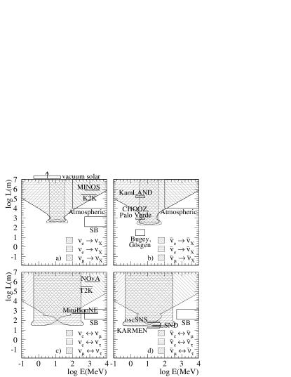
Figure 3: Oscillation probabilities in the $\log L$-$\log E$ plane for (a) $\nu$ disappearance, (b) $\bar{\nu}$ disappearance, (c) $\nu$ appearance, and (d) $\bar{\nu}$ appearance. In (a) and (b), the displayed regions have disappearance probability $P>10\%$. Regions for disappearance of different flavors are distinguished by different hatchings. In (c) and (d), the displayed regions have appearance probability $P>0.1\%$, and the regions for different flavors are again distinguished by different hatchings. Approximate $L$-$E$ sensitivity ranges for various oscillation experiments are displayed as labeled rectangles. In (a), the rectangle for solar neutrinos lies well above the plot, near $\log L\simeq 11$. Short-baseline experiments with $E\mathrel{\hbox to0.0pt{\lower 4.0pt\hbox{\hskip 1.0pt$\sim$}\hss}\raise 1.0pt\hbox{$>$}}1$ GeV are denoted SB.

Some generic predictions of the tandem model for typical experimental sensitivities are displayed in Fig. 3. These plots present information about appearance and disappearance probabilities in the $\log L$-$\log E$ plane for both neutrinos and antineutrinos. They provide an overview of the general predictions of the model and relate them to some existing and future experiments. Some details for the various classes of experiments are given in the following subsections.

In Figs. 3(a) and 3(b), regions above the curves correspond to disappearance probabilities greater than 10%. In Figs. 3(c) and 3(d), regions above the curves correspond to appearance probabilities greater than 0.1%. The figures also contain rectangles representing the regions of sensitivity of particular experiments. The tandem model predicts a signal in an experiment for oscillations of a particular type when its rectangle overlaps the region above the oscillation curve.

III.2.1 Solar

In the standard three-neutrino massive model, vacuum solar-neutrino oscillations show no energy dependence because $\Delta m^{2}_{\odot}\gg 10^{-10}$ eV² and the mixing matrix is energy independent. In the tandem model, however, the long-baseline limit of vacuum oscillations exhibits an energy dependence arising from the mixing matrix $U_{Ja}$, despite the loss of energy dependence in the factor $\sin^{2}(\Delta_{JK}L/2)$.

The $\nu_{e}$ survival probability on the energy scale relevant to the solar neutrino problem is shown in Fig. 4. This model yields an oscillation probability of $50\%$ for pp neutrinos, which have a continuous energy spectrum with endpoint at 0.420 MeV. The oscillation probability is also $50\%$ for ⁷Be neutrinos, which generate two monoenergetic lines with $90\%$ at 0.862 MeV and $10\%$ at 0.384 MeV. For the ⁸B neutrinos, which have a continuous energy spectrum with endpoint at 15.04 MeV, the model yields a probability of $\simeq 40\%$. These values are in reasonable agreement with the energy dependence observed in the existing solar-oscillation data.

In the tandem model, matter-enhanced oscillations msw play essentially no role in the description of solar neutrinos. In general, matter-enhanced solar-neutrino oscillations can be viewed as arising from an effective coefficient for Lorentz violation of the form km1 $(a_{L,{\rm eff}})_{ee}=\sqrt{2}G_{F}n_{e}$, where $n_{e}$ is the number density of electrons in the Sun. An analytical approximation for $n_{e}$ ssm yields $(a_{L,{\rm eff}})_{ee}\simeq 1.87\times 10^{-17}e^{-10.54R/R_{\odot}}$ MeV, where $R$ is the distance from the core and $R_{\odot}$ is the solar radius. In the tandem model, substantial effects can arise only if ${\mathaccent 23{c}}E\mathrel{\hbox to0.0pt{\lower 4.0pt\hbox{\hskip 1.0pt$\sim$}\hss}\raise 1.0pt\hbox{$<$}}(a_{L,{\rm eff}})_{ee}$, or $E\mathrel{\hbox to0.0pt{\lower 4.0pt\hbox{\hskip 1.0pt$\sim$}\hss}\raise 1.0pt\hbox{$<$}}0.5e^{-10.54R/R_{\odot}}$ MeV. For much of the solar-neutrino spectrum, this energy is too small to allow appreciable effects on the oscillation probability. This result is confirmed by numerical calculations.

We remark in passing that an interesting feature of the tandem model in the 10 MeV region is a reduced suppression of the $\bar{\nu}_{e}$ probability relative to that of $\nu_{e}$. This originates in CPT violation via the ${\mathaccent 23{a}}$ coefficient, and it may be relevant for $r$-process nucleosynthesis following core-collapse in supernovae qfmmww .

Figure 4: Solar-neutrino oscillation probabilities in the tandem model. (a) Curves representing survival probabilities for $\nu_{e}$ (solid), $\nu_{e}\rightarrow\nu_{\mu}$ (dashed), $\nu_{\mu}\rightarrow\nu_{\tau}$ (dotted), and $\nu_{\tau}\rightarrow\nu_{e}$ (dash-dotted). (b) Survival probability of $\nu_{e}$ in the tandem model (solid line) and in the standard three-neutrino massive model with a basic matter-induced effect (dashed). Note the different energy scales. The effects of experimental position and energy resolution are not shown.

III.2.2 Atmospheric

Figure 5: Survival probabilities for atmospheric neutrinos as a function of $L/E$ for (a) $\nu_{\mu}$ and (b) $\bar{\nu}_{\mu}$. Curves are shown for the tandem model (solid) and for the standard three-neutrino massive model (dashed). The effects of experimental position and energy resolution are not shown.

The atmospheric-neutrino results are well described by the tandem model. At high neutrino energies, the effective tandem hamiltonian for neutrinos becomes approximately

$$h^{\nu}_{\mathrm{TM}} \approx \left(\begin{array}[]{ccc}{\mathaccent 23{c}}E&~{}{\mathaccent 23{a}}&~{}{\mathaccent 23{a}}\\ {\mathaccent 23{a}}&~{}0&~{}{\mathaccent 23{a}}\\ {\mathaccent 23{a}}&~{}{\mathaccent 23{a}}&~{}0\end{array}\right),$$ (24)

with a similar simplification for $h^{\bar{\nu}}_{\mathrm{TM}}$. The ${\mathaccent 23{c}}$ and ${\mathaccent 23{a}}$ coefficients combine to produce a Lorentz-violating seesaw mechanism km1 , in which the model effectively reduces to a two-flavor limit with a pseudomass term km2 . The only significant probabilities are for the transitions $\nu_{\mu}\leftrightarrow\nu_{\tau}$ and $\bar{\nu}_{\mu}\leftrightarrow\bar{\nu}_{\tau}$, which involve $\Delta_{21}$ and are large only at energies above about 100 MeV. All amplitudes other than $U_{2\mu}U_{2\tau}U_{1\mu}U_{1\tau}$ approach zero at high energies.

A comparison of atmospheric-oscillation probabilities in the tandem model with those in the standard three-neutrino massive model is provided in Fig. 5. In both models, the disappearance probability is maximum in the region with $L/E=$ 300-600 m/MeV, which corresponds to the results reported by the Super-Kamiokande experiment Super-Kosc . This feature is common to both $\nu_{\mu}$-$\nu_{\tau}$ and $\bar{\nu}_{\mu}$-$\bar{\nu}_{\tau}$ oscillations. The tandem model contains CPT violation, but it is invisible in the high-energy region. These results are also consistent with the recent atmospheric measurement from the MINOS experiment MINOS .

III.2.3 Long-baseline reactor

At low neutrino energies, the effective tandem hamiltonian for antineutrinos becomes approximately

$$h^{\bar{\nu}}_{\mathrm{TM}} \approx \left(\begin{array}[]{ccc}0&~{}-{\mathaccent 23{a}}&~{}-{\mathaccent 23{a}}\\ -{\mathaccent 23{a}}&~{}0&~{}-{\mathaccent 23{a}}\\ -{\mathaccent 23{a}}&~{}-{\mathaccent 23{a}}&~{}{{{\mathaccent 23{m}}}^{2}}/2E\end{array}\right).$$ (28)

The component ${{{\mathaccent 23{m}}}^{2}}/2E$ creates another Lorentz-violating seesaw km1 . Here, it results in large $\bar{\nu}_{e}\leftrightarrow\bar{\nu}_{\mu}$ oscillations involving $\Delta_{21}$, with no contribution from other antineutrino flavors. The only oscillations are proportional to $U_{2e}U_{2\mu}U_{1e}U_{1\mu}$.

The oscillatory shape reported by the KamLAND experiment KamLANDosc is reproduced by the choice of values (20). Figure 6 shows the $\bar{\nu}_{e}$ survival probability as a function of energy and $L/E$.

Unlike the situation for atmospheric neutrinos, the CPT violation in the tandem model emerges in this $L$-$E$ range as a difference between $\nu_{e}$ and $\bar{\nu}_{e}$ survival probabilities. However, this difference is unobservable in the KamLAND experiment because the sources produce only $\bar{\nu}_{e}$. Note that the $\nu_{e}\rightarrow\nu_{\mu}$ oscillation probability is substantial only at low energies. This means the tandem model predicts a null signal for future long-baseline $\nu_{e}$-appearance experiments such as NOvA NOvA and T2K T2K .

Figure 6: Survival probabilities for long-baseline reactor antineutrinos. (a) Survival probabilities as a function of $E$ for $\bar{\nu}_{e}$ (solid), $\bar{\nu}_{e}\rightarrow\bar{\nu}_{\mu}$ (dashed), $\bar{\nu}_{\mu}\rightarrow\bar{\nu}_{\tau}$ (dotted), and $\bar{\nu}_{\tau}\rightarrow\bar{\nu}_{e}$ (dash-dotted). (b) Survival probabilities for $\bar{\nu}_{e}$ as a function of $L/E$ in the tandem model (solid) and in the standard three-neutrino massive model (dashed). The effects of experimental position and energy resolution are not shown.

III.2.4 Short-baseline reactor and accelerator

Experiment	Ref.	Oscillation channel	x Source x	x Baseline x	Energy	xx Status xx
Bugey	Bugey	$\bar{\nu}_{e}\rightarrow X$	reactor	15,40 m	3 MeV	null result
Gösgen	Gosgen	$\bar{\nu}_{e}\rightarrow X$	reactor	38, 46, 65 m	3 MeV	null result
Palo Verde	PaloVerde	$\bar{\nu}_{e}\rightarrow X$	reactor	750, 890 m	3 MeV	null result
CHOOZ	CHOOZ	$\bar{\nu}_{e}\rightarrow X$	reactor	1 km	3 MeV	null result
KARMEN	KARMEN	$\bar{\nu}_{\mu}\rightarrow\bar{\nu}_{e}$	accelerator	18 m	40 MeV	null result
LSND	LSND2	$\bar{\nu}_{\mu}\rightarrow\bar{\nu}_{e}$	accelerator	30 m	40 MeV	signal
OscSNS	OscSNS	$\bar{\nu}_{\mu}\rightarrow\bar{\nu}_{e}$	accelerator	60 m	40 MeV	planning
MiniBooNE	MiniBooNE	$\nu_{\mu}\rightarrow\nu_{e}$	accelerator	550 m	800 MeV	ongoing
CDHS	CDHS	$\nu_{\mu}\rightarrow X$	accelerator	130 m	1 GeV	null result
BNL-E776	BNLE776	$\nu_{\mu}\rightarrow\nu_{e}$, $\bar{\nu}_{\mu}\rightarrow\bar{\nu}_{e}$	accelerator	1 km	1.4 GeV	null result
CHORUS	CHORUS	$\nu_{\mu}\rightarrow\nu_{\tau}$	accelerator	600 m	27 GeV	null result
NOMAD	NOMAD	$\nu_{\mu}\rightarrow\nu_{\tau}$	accelerator	600 m	45 GeV	null result
CCFR	CCFR	$\nu_{\mu}\rightarrow\nu_{e}$, $\bar{\nu}_{\mu}\rightarrow\bar{\nu}_{e}$	accelerator	1 km	140 GeV	null result
NuTeV	NuTeV	$\nu_{\mu}\rightarrow\nu_{e}$, $\bar{\nu}_{\mu}\rightarrow\bar{\nu}_{e}$	accelerator	1 km	150 GeV	null result

Table 2: Recent and near-future experiments involving short-baseline oscillations at reactors and accelerators. The notation $\nu_{a}\rightarrow\nu_{b}$ indicates an appearance search, while $\nu_{a}\rightarrow X$ indicates a disappearance search.

Figure 7: Oscillation probabilities as a function of $E$ for neutrinos (solid) and antineutrinos (dashed) in (a) KARMEN, (b) LSND, (c) the proposed OscSNS experiment, and (d) the currently running MiniBooNE experiment. The effects of experimental position and energy resolution are not shown.

In recent years, many experiments with short baselines KARMEN ; LSND2 ; MiniBooNE ; Bugey ; Gosgen ; OscSNS ; PaloVerde ; CHOOZ ; CDHS ; CHORUS ; NOMAD ; BNLE776 ; CCFR ; NuTeV have searched for oscillations using neutrinos from reactor and accelerator sources. The results are summarized in Table 2. The predictions of the tandem model relevant at these baselines and energies are discussed in this subsection.

In the tandem model, oscillation probabilities at short baselines are typically small, so they are undetectable in reactor-disappearance experiments with sensitivities of order 10%. This can be seen from Fig. 3. Conceivably, a sensitive reactor experiment with a baseline of $\mathrel{\hbox to0.0pt{\lower 4.0pt\hbox{\hskip 1.0pt$\sim$}\hss}\raise 1.0pt\hbox{$>$}}$ 1 km might observe a signal predicted by the tandem model in the highest-energy bins of the $\bar{\nu}_{e}$ spectrum.

For short baselines $\mathrel{\hbox to0.0pt{\lower 4.0pt\hbox{\hskip 1.0pt$\sim$}\hss}\raise 1.0pt\hbox{$<$}}$ 1 km, oscillations of neutrinos at high energies $\mathrel{\hbox to0.0pt{\lower 4.0pt\hbox{\hskip 1.0pt$\sim$}\hss}\raise 1.0pt\hbox{$>$}}$ 100 MeV are strongly suppressed, as can also be seen from Fig. 3. The oscillation behavior in the high-energy region is similar to that of atmospheric neutrinos, and any experiments with high-energy neutrinos that are insensitive to atmospheric-parameter oscillations are also insensitive to oscillations in the tandem model.

In contrast, for short-baseline low-energy accelerator experiments, the nonzero mass term in the tandem model results in a small oscillation probability that lies on the edge of experimental sensitivity. The $\nu_{\mu}\rightarrow\nu_{e}$ and $\bar{\nu}_{\mu}\rightarrow\bar{\nu}_{e}$ oscillation probabilities for KARMEN, LSND, OscSNS, and MiniBooNE are shown in Fig. 7. The tandem model yields an oscillation probability on the order of 0.05-1% in the detectable energy range for all these experiments.

In particular, the model yields an acceptable value for the oscillation probability of $(0.264\pm 0.067\pm 0.045)\%$ reported by LSND. The oscillation probability is smaller for the KARMEN experiment due to the shorter baseline, and it lies below the experimental sensitivity. The tandem model predicts substantial appearance signals for $\nu_{e}$ and $\bar{\nu}_{e}$ in OscSNS and MiniBooNE. Note that these signals fall off rapidly with increasing energy.

IV Summary

In this work, we have constructed a model of neutrino oscillations involving only three degrees of freedom that describes all features of existing oscillation experiments, including the LSND result. This tandem model uses renormalizable terms in the SME, with one mass parameter and two coefficients for Lorentz violation. The value of the mass parameter is compatible with a conventional seesaw mechanism, and the coefficients for Lorentz violation have Planck-suppressed magnitudes that are consistent with the measurements recently reported by LSND. The observed solar-neutrino suppression and energy dependence are achieved without employing matter-enhanced oscillations.

The tandem model makes quantitative predictions that can be tested in the near future with results from the MiniBooNE experiment and from various planned short- and long-baseline appearance experiments such as OscSNS, NOvA, and T2K. There may also be subsidiary signals involving sidereal variations or other unconventional physics. In any case, the tandem model represents a candidate alternative to the standard three-neutrino massive model, and its existence reconfirms the key role of neutrino experiments in the ongoing exploration of physics beyond the Standard Model.

Appendix A Diagonalization

The general symmetric effective hamiltonian represented by the $3\times 3$ matrix

$$h_{\rm eff} = \left(\begin{array}[]{ccc}h_{ee}&h_{e\mu}&h_{\tau e}\\ h_{e\mu}&h_{\mu\mu}&h_{\mu\tau}\\ h_{\tau e}&h_{\mu\tau}&h_{\tau\tau}\end{array}\right)$$ (32)

can be analytically diagonalized, $h_{\rm eff}=U^{\dagger}E_{\rm eff}U$, by solving the cubic eigenvalue equation for the eigenvalues $E_{J}$ and then obtaining the diagonalizing matrix $U_{Ja}$. In the effective hamiltonians (13) and (17) for the tandem model, the entries are all real and given by $h_{ee}={\mathaccent 23{c}}E$, $h_{\mu\mu}=0$, $h_{\tau\tau}={{{\mathaccent 23{m}}}^{2}}/2E$, and $h_{e\mu}=h_{\tau e}=h_{\mu\tau}=\pm{\mathaccent 23{a}}$.

The first step is to solve the cubic eigenvalue equation. This takes the form

$$\lambda^{3}+a\lambda^{2}+b\lambda+c=0,$$ (33)

where

$$a = -{\rm{tr}}(h_{\mathrm{eff}}),$$

$$b = {\textstyle{1\over 2}}[{\rm{tr}}(h_{\mathrm{eff}})]^{2}-{\textstyle{1\over 2}}{\rm{tr}}(h_{\mathrm{eff}}^{2}),$$

$$c = -{\rm{det}}(h_{\mathrm{eff}}).$$ (34)

For the tandem model, these quantities are

$$a = -{\mathaccent 23{c}}E-{{{\mathaccent 23{m}}}^{2}}/2E,$$

$$b = {\mathaccent 23{c}}{{\mathaccent 23{m}}}^{2}/2-3{\mathaccent 23{a}}^{2},$$

$$c = {\mathaccent 23{a}}^{2}\left({\mathaccent 23{c}}E\mp 2{\mathaccent 23{a}}+{{{\mathaccent 23{m}}}^{2}}/2E\right).$$ (35)

Note that $b$ is energy independent and that CPT violation contributes only to the determinant quantity $c$.

It is convenient to introduce the combinations of $a$, $b$, and $c$ given by

$$Q = \textstyle{{{1}\over{9}}}(a^{2}-3b),$$

$$R = \textstyle{{{1}\over{54}}}(2a^{3}-9ab+27c),$$

$$\theta = \cos^{-1}\left({{R}\over{\sqrt{Q^{3}}}}\right).$$ (36)

In terms of these combinations, the energy eigenvalues $E_{J}$ can be expressed as

$$E_{1} = -2\sqrt{Q}\cos\left({{\theta}\over{3}}\right)-\textstyle{{{1}\over{3}}}a,$$

$$E_{2} = -2\sqrt{Q}\cos\left({{\theta+2\pi}\over{3}}\right)-\textstyle{{{1}\over{3}}}a,$$

$$E_{3} = -2\sqrt{Q}\cos\left({{\theta-2\pi}\over{3}}\right)-\textstyle{{{1}\over{3}}}a.$$ (37)

In general, the solution to the cubic (33) involves three unequal real eigenvalues $E_{J}$ provided the discriminant $D\equiv R^{2}-Q^{3}$ is negative definite. For the tandem model, the values (20) chosen for the model satisfy this condition for all neutrino energies $E$. With these values, the discriminant $D$ increases with $E$ to a maximum near 10 MeV, then decreases as $E$ increases. The appearance of the maximum around 10 MeV reflects the merger of the two Lorentz-violating seesaw mechanisms near that energy. Also, since the eigenvalues $E_{J}$ of the tandem-model effective hamiltonian are distinct for all energies $E$, no two eigenvalue differences $\Delta_{JK}$ coincide exactly for any given $E$. This fact is reflected in Figs. 2(a) and 2(a): if two eigenvalue differences were to coincide exactly then the logarithm of the third would diverge, a behavior absent from the figures.

The mixing matrix $U_{Ja}$ is found to take the form

$$U = \left(\begin{array}[]{ccc}{B_{1}C_{1}}/{N_{1}}&~{}{B_{2}C_{2}}/{N_{2}}&~{}{B_{3}C_{3}}/{N_{3}}\\ {C_{1}A_{1}}/{N_{1}}&~{}{C_{2}A_{2}}/{N_{2}}&~{}{C_{3}A_{3}}/{N_{3}}\\ {A_{1}B_{1}}/{N_{1}}&~{}{A_{2}B_{2}}/{N_{2}}&~{}{A_{3}B_{3}}/{N_{3}}\end{array}\right),$$ (41)

where

$$A_{J} = h_{\mu\tau}(h_{ee}-E_{J})-h_{\tau e}h_{e\mu},$$

$$B_{J} = h_{\tau e}(h_{\mu\mu}-E_{J})-h_{e\mu}h_{\mu\tau},$$

$$C_{J} = h_{e\mu}(h_{\tau\tau}-E_{J})-h_{\mu\tau}h_{\tau e},$$ (42)

and the normalization for each fixed $J$ is

$$N_{J} = \sqrt{A_{J}^{2}B_{J}^{2}+B_{J}^{2}C_{J}^{2}+C_{J}^{2}A_{J}^{2}}.$$ (43)

References

- (1) For recent conference proceedings including experimental aspects see, for example, V.A. Kostelecký, ed., CPT and Lorentz Symmetry III, World Scientific, Singapore, 2005; CPT and Lorentz Symmetry II, World Scientific, Singapore, 2002; CPT and Lorentz Symmetry, World Scientific, Singapore, 1999.
- (2) For recent reviews see, for example, R. Bluhm, hep-ph/0506054; D.M. Mattingly, Living Rev. Rel. 8, 5 (2005); G. Amelino-Camelia, C. Lämmerzahl, A. Macias, and H. Müller, AIP Conf. Proc. 758, 30 (2005).
- (3) V.A. Kostelecký and R. Potting, Phys. Rev. D 51, 3923 (1995).
- (4) D. Colladay and V.A. Kostelecký, Phys. Rev. D 55, 6760 (1997); Phys. Rev. D 58, 116002 (1998).
- (5) V.A. Kostelecký, Phys. Rev. D 69, 105009 (2004).
- (6) Particle Data Group, S. Eidelman et al., Phys. Lett. B 592, 1 (2004), and 2005 partial update for edition 2006.
- (7) B.T. Cleveland et al., Astrophys. J. 496, 505 (1998).
- (8) SAGE Collaboration, J.N. Abdurashitov et al., J. Exp. Theor. Phys. 95, 181 (2002).
- (9) GNO Collaboration, M. Altmann et al., Phys. Lett. B 490, 16 (2000).
- (10) Super-Kamiokande Collaboration, M.B. Smy et al., Phys. Rev. D 69, 011104 (2004).
- (11) SNO Collaboration, B. Aharmim et al., Phys. Rev. D 72, 052010 (2005).
- (12) MACRO Collaboration, M. Ambrosio et al., Eur. Phys. J. C 36, 323 (2004).
- (13) K2K Collaboration, E. Aliu et al., Phys. Rev. Lett. 94, 081802 (2005).
- (14) Super-Kamiokande Collaboration, Y. Ashie et al., Phys. Rev. Lett. 93, 101801 (2004).
- (15) MINOS Collaboration, P. Adamson et al., hep-ex/0512036.
- (16) KamLAND Collaboration, T. Araki et al., Phys. Rev. Lett. 94, 081801 (2005).
- (17) LSND Collaboration, A.A. Aguilar et al., Phys. Rev. D 64, 112007 (2001).
- (18) V.A. Kostelecký and M. Mewes, Phys. Rev. D 69, 016005 (2004).
- (19) V.A. Kostelecký and S. Samuel, Phys. Rev. D 39, 683 (1989); V.A. Kostelecký and R. Potting, Nucl. Phys. B 359, 545 (1991).
- (20) B. Altschul and V.A. Kostelecký, Phys. Lett. B 628, 106 (2005).
- (21) LSND Collaboration, L.B. Auerbach et al., Phys. Rev. D 72, 076004 (2005).
- (22) V.A. Kostelecký and M. Mewes, Phys. Rev. D 70, 076002 (2004).
- (23) KTeV Collaboration, H. Nguyen, in CPT and Lorentz Symmetry II, Ref. cpt04 .
- (24) FOCUS Collaboration, J.M. Link et al., Phys. Lett. B 556, 7 (2003).
- (25) BaBar Collaboration, B. Aubert et al., Phys. Rev. Lett. 92, 142002 (2004).
- (26) BELLE Collaboration, K. Abe et al., Phys. Rev. Lett. 86, 3228 (2001).
- (27) OPAL Collaboration, R. Ackerstaff et al., Z. Phys. C 76, 401 (1997).
- (28) DELPHI Collaboration, M. Feindt et al., preprint DELPHI 97-98 CONF 80 (1997).
- (29) V.A. Kostelecký, Phys. Rev. Lett. 80, 1818 (1998); Phys. Rev. D 61, 016002 (2000); Phys. Rev. D 64, 076001 (2001).
- (30) S.R. Coleman and S.L. Glashow, Phys. Rev. D 59, 116008 (1999).
- (31) V.D. Barger, S. Pakvasa, T.J. Weiler, and K. Whisnant, Phys. Rev. Lett. 85, 5055 (2000).
- (32) J.N. Bahcall, V. Barger, and D. Marfatia, Phys. Lett. B 534, 120 (2002).
- (33) A. de Gouvêa and C. Peña-Garay, Phys. Rev. D 71, 093002 (2005).
- (34) D. Hooper, D. Morgan, and E. Winstanley, Phys. Rev. D 72, 065009 (2005).
- (35) M.C. Gonzalez-Garcia, F. Halzen and M. Maltoni, Phys. Rev. D 71, 093010 (2005).
- (36) V.A. Kostelecký and M. Mewes, Phys. Rev. D 70, 031902(R) (2004).
- (37) L. Wolfenstein, Phys. Rev. D 17, 2369 (1978); S. Mikheev and A. Smirnov, Sov. J. Nucl. Phys. 42, 913 (1986); Sov. Phys. JETP 64, 4 (1986); Nuovo Cimento 9C, 17 (1986).
- (38) M. Gell-Mann, P. Ramond, and R. Slansky, in P. van Nieuwenhuizen and D.Z. Freedman, ed., Supergravity, North Holland, Amsterdam, 1979; T. Yanagida, in O. Sawada and A. Sugamoto, eds., Workshop on Unified Theory and the Baryon Number of the Universe, KEK, Japan, 1979; R. Mohapatra and G. Senjanović, Phys. Rev. Lett. 44, 912 (1980).
- (39) For a review see, for example, P. Langacker, Int. J. Mod. Phys. A18, 4015 (2003).
- (40) The Super-Kamiokande atmospheric data is fitted in M.D. Messier, CPT and Lorentz Symmetry III, Ref. cpt04 .
- (41) Q.G. Bailey and V.A. Kostelecký, gr-qc/0606030; V.A. Kostelecký and S. Samuel, Phys. Rev. Lett. 63, 224 (1989); Phys. Rev. D 40, 1886 (1989).
- (42) R. Bluhm and V.A. Kostelecký, Phys. Rev. D 71, 065008 (2005).
- (43) V.A. Kostelecký and R. Potting, Gen. Rel. Grav. 37, 1675 (2005).
- (44) Y. Grossman, C. Kilic, J. Thaler, and D.G.E. Walker, Phys. Rev. D 72, 125001 (2005).
- (45) R. Bluhm et al., Phys. Rev. D 68, 125008 (2003); Phys. Rev. Lett. 88, 090801 (2002); V.A. Kostelecký and M. Mewes, Phys. Rev. D 66, 056005 (2002).
- (46) V.A. Kostelecký and R. Lehnert, Phys. Rev. D 63, 065008 (2001).
- (47) W.H. Press, S.A. Teukolsky, W.T. Vetterling, and B.P. Flannery, Numerical Recipes in C++: The Art of Scientific Computing, Cambridge University Press, New York, 2002.
- (48) V.A. Kostelecký, C.D. Lane, and A.G.M. Pickering, Phys. Rev. D 65, 056006 (2002).
- (49) For a recent review, see R.N. Mohapatra and A.Y. Smirnov, hep-ph/0603118.
- (50) For recent textbooks discussing these issues see, for example, M. Fukugita and T. Yanagida, Physics of Neutrino and Applications to Astrophysics, Springer, New York, 2003; R.N. Mohapatra and P. Pal, Massive Neutrinos in Physics and Astrophysics, World Scientific, Singapore, 2004.
- (51) An early discussion of a model of this type is M. Fukugita, T. Yanagida, and M Yoshimura, Phys. Lett. B 106, 183 (1981).
- (52) For a recent review see, for example, M. Tegmark, hep-ph/0503257.
- (53) J.N. Bahcall, M.H. Pinsonneault, and S. Basu, Astrophys. J. 555, 990 (2001).
- (54) The effects on the -process of an enhancement of relative to are discussed in Y.-Z. Qian, G.M. Fuller, G.J. Mathews, R.W. Mayle, J.R. Wilson, and S.E. Woosley, Phys. Rev. Lett. 71, 1965 (1993). For a recent review see, for example, Y.-Z. Qian, Prog. Part. Nucl. Phys. 50, 153 (2003).
- (55) NOvA Collaboration, D.S. Ayres et al., hep-ex/0503053.
- (56) Y. Itow et al., arXiv:hep-ex/0106019.
- (57) Y. Declais et al., Nucl. Phys. B 434, 503 (1995).
- (58) G. Zacek et al. Phys. Rev. D 34, 2621 (1986).
- (59) F. Boehm et al., Phys. Rev. D 64, 112001 (2001).
- (60) M. Apollonio et al., Eur. Phys. J. C 27, 331 (2003).
- (61) KARMEN Collaboration, B. Armbruster et al. Phys. Rev. D 65, 112001 (2002).
- (62) G.T. Garvey et al., Phys. Rev. D 72, 092001 (2005).
- (63) MiniBooNE Collaboration, R. Tayloe, Nucl. Phys. Proc. Suppl. 118, 157 (2003).
- (64) F. Dydak et al., Phys. Lett. B 134, 281 (1984).
- (65) L. Borodovsky et al., Phys. Rev. Lett. 68, 274 (1992).
- (66) CHORUS Collaboration, E. Eskut et al. Phys. Lett. B 497 (2001) 8.
- (67) NOMAD Collaboration, P. Astier et al., Nucl. Phys. B 611, 3 (2001).
- (68) CCFR/NuTeV Collaboration, A. Romosan et al., Phys. Rev. Lett. 78, 2912 (1997).
- (69) S. Avvakumov et al., Phys. Rev. Lett. 89, 011804 (2002).