INTRODUCTION TO EXTRA DIMENSIONS 

The aim of this talk is to provide non-experts with a brief and elementary introduction on the field of extra dimensions. The main motivation for extra dimensions relies on the more fundamental string theories that predict ten (or eleven) space-time dimensions. Extra dimensions must be compactified and there appear branes where gauge and/or gravity propagates. Compactification relates string constants (string scale and string coupling) with four-dimensional constants (Planck scale and gauge coupling). Only gravity can propagate in dimensions transverse to the brane. They can be detected either by gravitational (table-top) or by collider experiments where Kaluza-Klein graviton production appears as missing energy. Transverse dimensions can be as large as the sub-millimeter. Ordinary matter can also propagate in dimensions parallel to the brane. It can give rise to bumps in the dilepton invariant mass in hadron colliders or contribute by indirect effects to the electroweak observables. Longitudinal dimensions can be probed at LHC up to a scale of 6.7 TeV (9 TeV) for one (two) extra dimension(s). Extra dimensions also give rise to new theoretical ideas related to supersymmetry and electroweak breaking. Some of these ideas are reviewed.

1 Introduction

These notes contain very elementary and introductory material on the field of (large) extra dimensions mainly addressed to non-expert theorists and experimentalists wishing to initiate themselves in the subject. Although this author has contributed to some of the original developments that will be reviewed, no effort will be made for originality here.

Extra dimensions were introduced to solve classical problems of Particle Physics. Mainly to solve the hierarchy problem. Here two main avenues were open.

$\bullet$ If there is a “warped” extra dimension, large scales at the Planck brane are redshifted at the TeV brane $\!{}^{{\bf?}}$ as it is shown in the cartoon of Fig. 1 (left panel). The (RS) relationship between the weak and Planck scales is given by

$$M_{W}=e^{-2k\pi R}M_{P\ell}$$ (1)

$\bullet$ If there are $n$ very large extra dimensions where only gravity propagates the Planck scale is “reduced” by the large compactification volume $V\sim R^{n}$. In this case the (ADD) relation between weak and Planck scales is $\!{}^{{\bf?}}$

$$M_{W}\simeq\left[M_{Pl}\,R\right]^{-\frac{n}{n+2}}M_{Pl}$$ (2)

This solution is illustrated in the right panel of Fig. 1.

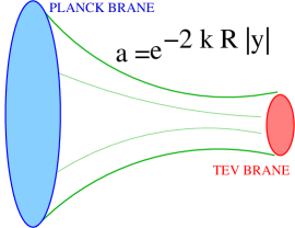
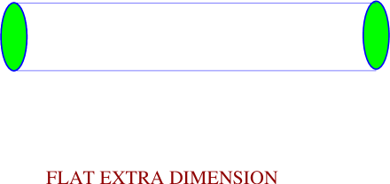
Figure 1: Left panel: The RS solution to the hierarchy; $a$ is the warp factor, $k$ is the AdS curvature and $R$ the compactified radius. Right panel: The ADD solution to the hierarchy.

2 Where do extra dimensions come from?

For a consistent quantum theory description of gravity we must abandon the concept of particle and instead introduce that of string $\!{}^{{\bf?}}$. Strings and in particular superstrings will lead, as we will see, to the existence of extra dimensions. In fact a string is a generalization of a “point particle”. While the latter is described, when propagating in the space-time, by a world line $X^{\mu}=X^{\mu}(\tau)$, where $\tau$ is the proper time of the particle, a string is a one-dimensional spatially extended object that, when propagating in D space-time dimensions, spans a world sheet $X^{\mu}=X^{\mu}(\xi^{\alpha}),\quad\xi^{\alpha}=(\tau,\sigma)$, where now there are a proper time $\tau$ and a proper space $\sigma$. Strings can be open or closed in the proper space direction $\sigma$, as shown in Fig. 2.

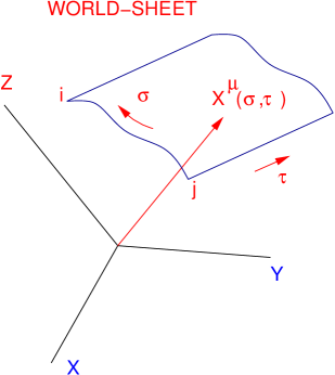
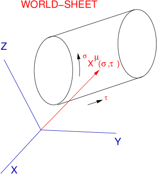
Figure 2: Left panel: The world sheet of an OPEN string propagating in the space-time. Right panel: The world sheet of a CLOSED string.

The cancellation of the conformal anomaly leads to a critical value of the space-time dimensionality. In the case of supersymmetric strings it is given by $D=10$ ($D=11$ for M-theory $\!{}^{{\bf?}}$). There are then six extra dimensions on top of the four flat ones that we experience. The six extra dimensions must be compactified and the size of their radii is constrained by experimental data, as we will see. The existence of extra (compactified) spatial dimensions is the first remarkable feature of string theories.

3 Strings and branes

The second great feature of string theories is that they predict the existence of subsurfaces of the whole space or “branes”. In particular $Dp$-branes are $(p+1)$-dimensional subsurfaces where open strings can end. Extra dimensions can then be either LONGITUDINAL or TRANSVERSE to the branes. Technically speaking longitudinal directions are those where the string has Neumann boundary conditions while on transverse directions the string has Dirichlett boundary conditions. In other words open string ends can move along longitudinal (Neumann) coordinates and therefore they have Kaluza-Klein (KK) modes with respect to them while they are fixed at transverse (Dirichlett) coordinates and have winding modes ($\omega$) depending on the number of times the string winds around the transverse (compact) coordinate. Closed strings propagate in the bulk. These situations are illustrated in Fig. 3

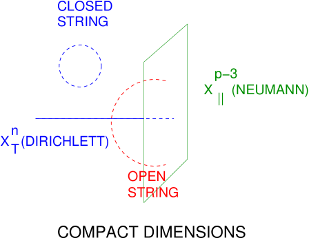
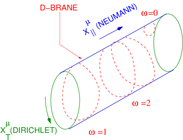
Figure 3: Open and closed strings propagating in extra dimensions. Closed strings propagate in the bulk (left panel). Open strings propagate with ends at $X_{T}=$constant for different windings (right panel) while they depend on $X_{L}\equiv X_{||}$.

To make contact with experiments we will describe the different string theories from the point of view of effective field theories. The parameters are

$\bullet$ $String\ scale\quad{\Rightarrow}\quad M_{s}=\ell_{s}^{-1}$, where $\alpha^{\prime}\sim 1/M_{s}^{2}$ is the string tension.

$\bullet$ $String\ coupling\quad{\Rightarrow}\quad\lambda_{s}=e^{\langle\phi\rangle}$, where $\phi$ is the dilaton field.

$\bullet$ COMPACTIFICATION $10D\Rightarrow 4D\otimes V_{6}$

$\bullet$ $Planck\ scale\quad{\Rightarrow}\quad M_{P}=\ell_{P}^{-1}$

$\bullet$ $Gauge\ coupling\quad{\Rightarrow}\quad g$

The massless modes of open and closed strings describe the physical degrees of freedom of our four-dimensional effective theories. In particular

$\bullet$ Closed strings describe gravity

$\bullet$ Open strings with ends bounded to propagate on Dp-branes describe gauge interactions.

The relationship between the string parameters, string scale ($M_{s}$) and the string coupling ($\lambda_{s}$), and the four-dimensional parameters, Planck scale ($M_{P\ell}$) and unified gauge coupling ($g$) is provided by the compactification from ten to four dimensions. The six internal compact dimensions are [p-3] (longitudinal) and [n=(9-p)](transverse). The ten-dimensional effective action can be written as (the different powers of string parameters are easily obtained)

$$S=\int_{{bulk}}d^{10}x\frac{1}{\lambda_{s}^{2}}\ell_{s}^{-8}\mathcal{{R}}+\int_{{brane}}d^{p+1}x\frac{1}{\lambda_{s}}\ell_{s}^{3-p}{F^{2}}$$ (3)

Upon compactification of extra dimensions the following relations between string and four-dimensional parameters follow

$$\frac{1}{\ell_{P}^{2}}=\frac{V_{L}V_{T}}{\lambda_{s}^{2}\ell_{s}^{8}}\qquad\frac{1}{g^{2}}=\frac{V_{L}}{\lambda_{s}\ell_{s}^{p-3}}$$ (4)

and rescaling the longitudinal volume as $V_{L}\equiv v_{L}\ell_{s}^{p-3}$ one gets the final relation

$$M_{P}^{2}=\frac{1}{g^{4}v_{L}}M_{s}^{2+n}R_{T}^{n}\qquad\lambda_{s}=g^{2}v_{L}$$ (5)

Defining now the (4+n) Planck scale $M_{*}$ as $M_{*}^{2+n}=M_{s}^{2+n}/g^{4}v_{L}$ one can finally write the ADD relation as

$$M_{P}^{2}=M_{*}^{2+n}R_{T}^{n}$$ (6)

4 Experimental detection

If $M_{s}\sim M_{*}\sim$ few TeV string excitations can be at reach at LHC. On the other hand the ADD relation can “explain” the weakness of gravitational interactions by the size of extra-large transverse dimensions $1/R_{T}\ll 1$ TeV. Both transverse and longitudinal dimensions (i. e. their Kaluza-Klein excitations) can be at reach at experiments:

$\bullet$ Kaluza-Klein excitations of transverse dimensions $R_{T}$ can affect gravitational (and collider) experiments.

$\bullet$ Kaluza-Klein excitations of longitudinal dimensions with size $1/R_{L}\sim$ few TeV can be detected at LHC.

4.1 Transverse dimensions

Only gravity propagates in transverse extra dimensions. Therefore these dimensions can be extra-large. Let $R_{T}$ be the (common) radius of transverse dimensions where gravity propagates. The ADD relation (6) relates the scales of quantum gravity in the higher dimensional theory and the transverse radius. For instance for a value of the fundamental scale $M_{*}=2$ TeV the value of the common transverse radius $R_{T}$ depends on the different possible dimensionalities ($n$) of the transverse space. This is illustrated in Table 1.

Table 1: The prediction of the transverse radius for different dimensions of the transverse space

n	1	2	6
$R_{T}$	$10^{7}$ Km	0.2 mm	0.1 fm
	excluded	barely	consistent
		consistent

As we can see from Table 1 the case of $n=1$ transverse dimension is excluded while the case of $n=2$ is barely consistent with table-top gravitational experiments.

– Gravitational experiments

Extra dimensions produce deviations from Newton’s law. They can be parametrized in the following way:

$$V(r)=\left\{\begin{array}[]{l}-\frac{G_{N}}{r}\left(1+\alpha e^{-r/R_{T}}+\cdots\right),\ r\geq R_{T}\\ -\frac{G_{N}^{(4+n)}}{r^{1+n}},\ r\ll R_{T}\end{array}\right.$$ (7)

Present gravitational experiments place the lower bounds on $R_{T}$ in the sub-millimeter region. Some recent experimental results can be found in Ref. $\!{}^{{\bf?}}$. These bounds appear in the typical way shown in Fig. 4.

Figure 4: Limit on non-Newtonian forces at short distances as a function of their range $\lambda$ and their strength relative to gravity $\alpha$. Present bounds are in the sub-millimeter region.

– Collider signatures

Transverse extra dimensions can also be detected in high-energy colliders. The signatures are based on missing energy in reactions corresponding to the production of KK-gravitons in the bulk. For instance

$$e^{+}e^{-}\longrightarrow\gamma{\displaystyle\sum_{k}}G^{(k)}$$ (8)

Every single graviton couples gravitationally $\sim 1/M_{P}^{2}$ but the large amount of gravitons cancels (using ADD relation) the $M_{P\ell}^{2}$ dependence

$$\sigma\sim s^{n/2}/M_{*}^{n+2}$$ (9)

The 95% confidence limits on $R_{T}$ [cm] and $M_{*}$ [GeV] have been computed in Ref. $\!{}^{{\bf?}}$, where $R_{T}$ and $M_{*}$ are related by the ADD relation. For present or past accelerators the results are (depending on the dimensionality of the extra space) given in Table 2.

Table 2: Bounds on $M_{*}$ [GeV] and $R_{T}$ [cm] from LEP2 and Tevatron

Collider	$R_{T}$ / $M_{*}$ ($n=2$)	$R_{T}$ / $M_{*}$ ($n=6$)
LEP2	$4.8\times 10^{-2}$ / 1200	$6.9\times 10^{-12}$ / 520
Tevatron	$11.0\times 10^{-2}$ / 750	$5.8\times 10^{-12}$ / 610

For future accelerators (as the LHC and the ILC) the bounds obtained in $\!{}^{{\bf?}}$ range for $M_{*}$, between 8 TeV (for $n=2$) and 3 TeV (for $n=6$), and for $R_{T}$ between $10^{-3}$ cm (for $n=2$) and $10^{-13}$ cm (for $n=6$).

4.2 Longitudinal directions

Longitudinal directions are those where the Standard Model (SM) fields can propagate. In this picture the SM fields propagate in a brane, with p-3 longitudinal dimensions wrapped on a compact space (orbifold) with 4D boundaries at the fixed points. The cartoon of the brane looks like in Fig. 5.

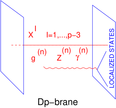
Figure 5: A $p$-brane where SM fields propagate. We will consider that the gauge sector is propagating in the bulk of the extra dimensions while the quark and lepton sector is localized at the orbifold fixed points.

– Indirect detection

The indirect detection of longitudinal extra dimensions is based on the modification of EW observables $(M_{W},\,\Gamma_{\ell\ell},\,\Gamma_{had},\,A_{FB}^{\ell},\,Q_{W},\,\dots)$ by the exchange of KK-modes $Z^{(n)}$, $\gamma^{(n)}$, as it is shown in the picture of Fig. 6.

Electroweak precision tests provide bounds on the compactification scale $M_{c}=1/R$ that are model dependent and in all cases of order a few TeV. To give an idea of the model dependence of the result we present in Fig. 7 the bounds on $M_{c}$ as a function of $\sin^{2}\beta$ (where $\tan\beta=v_{2}/v_{1}$) for the different models analyzed in Ref. $\!{}^{{\bf?}}$. For more details see Ref. $\!{}^{{\bf?}}$.

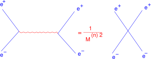
Figure 6: Fermions localized on the brane couple to KK modes and give rise to an effective six-dimensional operator.

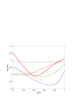
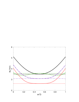
Figure 7: Lower bounds on $M_{c}$ in five-dimensional models from electroweak precision tests.

– Direct detection

Direct detection is based on production of KK modes from $f\bar{f}$ and subsequent decay into a pair of fermions. For instance in hadron colliders (as Tevatron or LHC) it will proceed through Drell-Yan processes as that presented in Fig. 8.

The direct production of KK-modes through Drell-Yan processes will in turn produce two effects. One is that it will increase the number of events with respect to the Standard Model prediction. For instance for the LHC collider and a given number of extra dimensions ($D=1,2$) one can predict the excess in the number of events $(N_{N}^{\rm SM})/\sqrt{N^{\rm SM}}$ as a function of the longitudinal radius $R_{L}$ as in the left panel of Fig. 9 $\!{}^{{\bf?}}$. One can see that, depending on the number of extra dimensions, one can reach 9 TeV for the 95 % confidence level bounds. The other effect is when the resonance is detected and produces a bump on the invariant mass of the final states. This one is the “golden channel” to discover an extra gauge boson. In the case of KK excitations, and depending on the compactification radius, one can even detect the first two-KK modes for the case of one extra dimension as shown in the right panel of Fig. 9.

We will conclude this section by summarizing in Table 3 the largest compactification scales that can be probed at 95 % confidence level for one extra dimension and different colliders.

Table 3: Highest compactification scales at reach for one extra dimension.

Collider	LEP2	ILC-500	ILC-1000	Tevatron	LHC
$M_{c}$ (TeV)	1.9	8	13	1.2	6.7

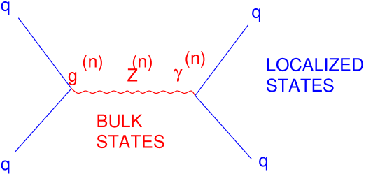
Figure 8: Drell-Yan process through exchange of the KK mode of a gluon, electroweak gauge boson or photon.

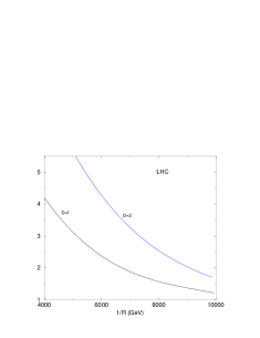
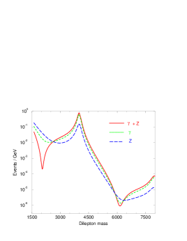
Figure 9: Left panel: Excess of lepton pair events at LHC for dilepton invariant mass above 400 GeV from $D=1,2$ extra dimensions. Right panel: Production at LHC of $\gamma$ and $Z$ Kaluza-Klein excitations.

5 New theoretical ideas from extra dimensions

Extra dimensions also exhibit the feature of providing NEW solutions to OLD problems in Particle Physics. These solutions mainly concern the problem of supersymmetry breaking as well as electroweak symmetry breaking. In this section we will cover a sample of possibilities and will leave aside others (as e. g. Higgsless models). Our selection is biased by our own experience and does not reflect at all any scientific preference.

5.1 Supersymmetry breaking

$\bullet$ Supersymmetry can be broken on the fixed points by orbifold boundary conditions $\!{}^{{\bf?}}$: the number of supersymmetries on the branes is halved. For instance in the case of one or two extra dimensions compactified on orbifolds the number of supersymmetries of zero modes is

$N=2\quad{\Rightarrow}\quad N=1$

$\bullet$ Supersymmetry can be further broken by twisted boundary conditions: the so-called Scherk-Schwarz breaking $\!{}^{{\bf?}}$. Then in the effective four-dimensional theory

$N=1\quad{\Rightarrow}\quad N=0$

$\bullet$ In particular if gauginos (and squarks) propagate in the bulk of extra dimensions they acquire masses proportional to the compactification scale

$M_{1/2}\sim 1/R$

5.2 Gauge-Higgs unification

It is possible to unify the Higgs and gauge sectors by using for the former the extra dimensional components of the higher-dimensional gauge bosons: this is called gauge-Higgs unification

$A_{\mu}^{\alpha}={\rm gauge\ bosons},\\ A_{i}^{\alpha}={\rm Higgses};\ \ {\alpha\in{\rm Adjoint}}$

The two main features of the gauge-Higgs unification are:

$\bullet$ It requires to enlarge the SM gauge group e. g. $\!{}^{{\bf?}}$

$SU(3)\to SU(2)\otimes U(1)$

$\bullet$ This is an alternative solution to the hierarchy problem because the extra dimensional gauge theory protects the Higgs mass from quadratic divergences $\!{}^{{\bf?}}$.

$\bullet$ Electroweak breaking proceeds via the Hosotani mechanism $\!{}^{{\bf?}}$ (Wilson line). For instance in the simplest model $\!{}^{{\bf?}}$

$A_{\mu}^{SU(2)\otimes U(1)}$= SM gauge bosons

$A_{i}^{SU(3)/SU(2)\otimes U(1)}$= SM Higgs bosons

$\bullet$ The Higgs mass parameter becomes tachyonic radiatively

$m_{H}^{2}\sim-({\rm loop\ factor})\ 1/R^{2}$

$\bullet$ It is difficult to obtain realistic models: quadratically divergent localized tadpoles can appear, Higgs mass requires more than five dimensions, fermion masses are difficult to obtain, …

5.3 Higgs Electroweak Symmetry Breaking

By using the Scherk-Schwarz mechanism to break supersymmetry and the matter localized on the four-dimensional boundary (gaugino mediated supersymmetry breaking) $\!{}^{{\bf?}}$ one can obtain a realistic and very peculiar model of electroweak symmetry breaking $\!{}^{{\bf?}}$. This model has the following nice features:

$\bullet$ Models are of ”no-scale” type and then no anomaly mediated supersymmetry breaking occurs.

$\bullet$ No one-loop quadratic or linear sensitivity on the cutoff $\Lambda$ of Higgs masses.

$\bullet$ Gauginos are the heaviest supersymmetric particles (they are in the TeV or multi-TeV region).

$\bullet$ EWSB is triggered by tachyonic tree-level masses and two-loop radiative corrections.

$\bullet$ Squarks and sleptons acquire radiative masses from gluinos and electroweak gauginos, respectively. In fact there is a “fixed” mass relation that can be considered as the smoking gun of these models. It is given by

$$(m_{\tilde{q}_{L}},\,m_{\tilde{u}_{R}},\,m_{\tilde{d}_{R}},\,m_{\tilde{\ell}_{L}},\,m_{\tilde{e}_{R}})\simeq\\ (0.110,\,0.103,\,0.102,\,0.042,\,0.025)\sin\pi\omega/R$$ (10)

where the SS parameter is $\omega=M_{\tilde{g}}R$.

$\bullet$ Charged and neutral Higgsinos are almost degenerate with mass splittings $\sim 1$ GeV.

$\bullet$ Fine-tuning of MSSM alleviated.

$\bullet$ The LSP is a neutralino which is a good candidate to Dark Matter.

6 Conclusions

We will conclude with a few obvious observations:

• Large extra dimensions are well motivated theoretically.

• Large extra dimensions and low scale quantum gravity effects are at reach at present (Tevatron) and future (LHC) colliders.

• Large extra dimensions have unambiguous experimental signatures.

• Large extra dimensions can also help to solve theoretical Particle Physics problems (electroweak breaking, hierarchy, flavor,…).

• If extra dimensions are found at LHC it would possibly constitute the most important revolution in the History of Particle Physics!

References

References

- [1] L. Randall and R. Sundrum, Phys. Rev. Lett. 83 (1999) 3370 [arXiv:hep-ph/9905221].
- [2] N. Arkani-Hamed, S. Dimopoulos and G. R. Dvali, Phys. Lett. B 429 (1998) 263 [arXiv:hep-ph/9803315].
- [3] M. B. Green, J. H. Schwarz and E. Witten, “Superstring Theory. Vol. 1: Introduction, and Vol. 2: Loop Amplitudes, Anomalies And Phenomenology,”
- [4] P. Horava and E. Witten, Nucl. Phys. B 475 (1996) 94 [arXiv:hep-th/9603142].
- [5] S. J. Smullin, A. A. Geraci, D. M. Weld, J. Chiaverini, S. Holmes and A. Kapitulnik, “New constraints on Yukawa-type deviations from Newtonian gravity at 20-microns,” Phys. Rev. D 72 (2005) 122001 [Erratum-ibid. D 72 (2005) 129901] [arXiv:hep-ph/0508204]; C. D. Hoyle, D. J. Kapner, B. R. Heckel, E. G. Adelberger, J. H. Gundlach, U. Schmidt and H. E. Swanson, “Sub-millimeter tests of the gravitational inverse-square law,” Phys. Rev. D 70 (2004) 042004 [arXiv:hep-ph/0405262]; J. C. Long, H. W. Chan, A. B. Churnside, E. A. Gulbis, M. C. M. Varney and J. C. Price, “Upper limits to submillimeter-range forces from extra space-time dimensions,” Nature 421 (2003) 922.
- [6] E. A. Mirabelli, M. Perelstein and M. E. Peskin, Phys. Rev. Lett. 82 (1999) 2236 [arXiv:hep-ph/9811337].
- [7] A. Delgado, A. Pomarol and M. Quiros, JHEP 0001 (2000) 030 [arXiv:hep-ph/9911252].
- [8] I. Antoniadis, K. Benakli and M. Quiros, Phys. Lett. B 331 (1994) 313 [arXiv:hep-ph/9403290]; I. Antoniadis, K. Benakli and M. Quiros, Phys. Lett. B 460 (1999) 176 [arXiv:hep-ph/9905311].
- [9] L. J. Dixon, J. A. Harvey, C. Vafa and E. Witten, Nucl. Phys. B 261 (1985) 678; L. J. Dixon, J. A. Harvey, C. Vafa and E. Witten, Nucl. Phys. B 274 (1986) 285.
- [10] J. Scherk and J. H. Schwarz, Phys. Lett. B 82 (1979) 60; J. Scherk and J. H. Schwarz, Nucl. Phys. B 153 (1979) 61.
- [11] I. Antoniadis, K. Benakli and M. Quiros, New J. Phys. 3 (2001) 20 [arXiv:hep-th/0108005].
- [12] Y. Hosotani, Phys. Lett. B 126 (1983) 309; Y. Hosotani, Phys. Lett. B 129 (1983) 193.
- [13] A. Pomarol and M. Quiros, Phys. Lett. B 438 (1998) 255 [arXiv:hep-ph/9806263]; I. Antoniadis, S. Dimopoulos, A. Pomarol and M. Quiros, Nucl. Phys. B 544 (1999) 503 [arXiv:hep-ph/9810410]; A. Delgado, A. Pomarol and M. Quiros, Phys. Rev. D 60 (1999) 095008 [arXiv:hep-ph/9812489].
- [14] D. Diego, G. von Gersdorff and M. Quiros, JHEP 0511 (2005) 008 [arXiv:hep-ph/0505244]; D. Diego, G. von Gersdorff and M. Quiros, arXiv:hep-ph/0605024.