TUM-HEP-634/06

MADPH-06-1459

Optimization of a neutrino factory oscillation experiment

P. Huber,  M. Lindner,  M. Rolinec,  W. Winter

Department of Physics, University of Wisconsin,

1150 University Avenue, Madison, WI 53706, USA

^,Physik–Department, Technische Universität München,

James–Franck–Strasse, 85748 Garching, Germany

Max–Planck–Institut für Kernphysik,

Postfach 10 39 80, 69029 Heidelberg, Germany

School of Natural Sciences, Institute for Advanced Study,

Einstein Drive, Princeton, NJ 08540, USA

We discuss the optimization of a neutrino factory experiment for neutrino oscillation physics in terms of muon energy, baselines, and oscillation channels (gold, silver, platinum). In addition, we study the impact and requirements for detector technology improvements, and we compare the results to beta beams. We find that the optimized neutrino factory has two baselines, one at about $3\,000$ to $5\,000\,\mathrm{km}$, the other at about $7\,500\,\mathrm{km}$ (“magic” baseline). The threshold and energy resolution of the golden channel detector have the most promising optimization potential. This, in turn, could be used to lower the muon energy from about $50\,\mathrm{GeV}$ to about $20\,\mathrm{GeV}$. Furthermore, the inclusion of electron neutrino appearance with charge identification (platinum channel) could help for large values of $\sin^{2}2\theta_{13}$. Though tau neutrino appearance with charge identification (silver channel) helps, in principle, to resolve degeneracies for intermediate $\sin^{2}2\theta_{13}$, we find that alternative strategies may be more feasible in this parameter range. As far as matter density uncertainties are concerned, we demonstrate that their impact can be reduced by the combination of different baselines and channels. Finally, in comparison to beta beams and other alternative technologies, we clearly can establish a superior performance for a neutrino factory in the case $\sin^{2}2\theta_{13}\lesssim 0.01$.

1 Introduction

Neutrino oscillation physics has entered the precision age by the measurements of the leading atmospheric and solar oscillation parameters. The status of current data and parameter estimates can be found, e.g., in Refs. [1, 2]. The common framework typically used for neutrino oscillations includes three active flavors, which can accommodate all data besides the LSND evidence [3]. The rough picture is that there are two mass splittings which are different by a factor of $\sim 30$, as well as one possibly maximal mixing angle, and one large, but certainly not maximal, mixing angle. The third mixing angle is known to be not larger than the Cabibbo angle. That leaves a number of open questions even within the standard framework: The value of the small mixing angle $\theta_{13}$, the ordering of the mass eigenstates, the value of the Dirac-type CP phase, and whether there is maximal mixing in the neutrino sector. A number of experiments in the near future are targeted towards providing answers to some of those questions. They all have in common that they only will succeed for values of $\sin^{2}2\theta_{13}$ not too much below the current bound. Examples are future reactor experiments with near and far detectors [4, 5, 6, 7] and neutrino beams [8, 9, 10]. Since none of them will be able to provide more than indications and hints towards the mass hierarchy and leptonic CP violation, there will be the need for an advanced neutrino oscillation facility. It will allow to make firm statements and precise measurements in order to finally reveal the underlying theoretical structures. There is a large number of contenders for this advanced neutrino facility, but it seems there is consensus that the most capable of these are neutrino factories [11, 12, 13] and higher gamma beta beams [14, 15]. They will allow for high precision measurements for large $\sin^{2}2\theta_{13}$, or will have excellent discovery reaches for small values of $\sin^{2}2\theta_{13}$.

In this study, we focus on the optimization and physics reach of a neutrino factory. Earlier studies discussing the potential and optimization of such an experiment include Refs. [16, 17, 18, 19]. We extend those results by including the full parameter correlations, degenerate solutions, the matter density uncertainty as well as detector effects, backgrounds and systematical errors in the analysis. We investigate the continuous dependence of the performance on $L$ and $E_{\mu}$ as well. In addition, we improve on the use of disappearance information by using a data sample without charge identification, we test the combination of baselines, and we discuss different channels and improvements to the detection system. The objective of this work is to identify the “optimal” setup given current possibilities and to determine the factors which have the greatest potential for improvement. Based on that, we will formulate the requirements which upgrades of a neutrino factory should fulfill in order to yield a certain level of performance gain. These requirements will allow to focus R&D for further optimization in the coming years.

In order to optimize the neutrino factory, we consider the sensitivities to $\sin^{2}2\theta_{13}$, the mass hierarchy, and CP violation, as well as we discuss measurement of the leading atmospheric parameters. For the underlying oscillation theory, we assume unitary three-flavor neutrino oscillations without significant “new physics” effects, since there is so far no convincing evidence for such effects. However, note that the physics motivation for a neutrino factory does include many more measurements than discussed in this study, some of which may lead to a very different optimization. Already from the point of view of oscillation physics, an important application, which is not discussed here, are precision measurements of $\sin^{2}2\theta_{13}$ and $\delta_{\mathrm{CP}}$, as soon as $\sin^{2}2\theta_{13}>0$ is established (see, e.g., Refs. [20, 21]). Furthermore, the issue of whether $\theta_{23}$, if it is not maximal, is smaller or larger than $\pi/4$ (octant) is an important question [22]. Furthermore, using a very long baseline $L\gtrsim 5\,000\,\mathrm{km}$, one can verify the MSW effect at high significance [17, 23] even for $\sin^{2}2\theta_{13}=0$ by the solar appearance term [24]. In addition, a baseline $L\simeq 6\,000\,\mathrm{km}$ could be required for the mass hierarchy determination for $\sin^{2}2\theta_{13}=0$ using disappearance information [25, 26], and the possible application of a matter density measurement may have some impact on the baseline choice as well [27]. Except from standard three-flavor oscillation, another important category are “new physics” tests, where a large volume of literature exists, see, e.g., Refs. [28, 29, 30, 31, 32, 33, 34, 35, 36, 37, 38]. For a discussion of present bounds on non-standard neutrino interactions, see Ref. [39]. In addition, the neutrino factory front-end can be used for high statistics muon and neutrino physics experiments [40]. Therefore, the physics motivation for a neutrino factory does not only depend on the measurements discussed in this study, but is based on a much wider range of physics. Obviously, the “optimal” neutrino factory for testing new physics effects may be completely different from the one found as optimal with respect to, for instance, CP violation. This should be kept in mind in interpreting our results.

This study is organized as follows: In Section 2 we describe the neutrino oscillation phenomenology in terms of oscillation probabilities, we discuss the impact of using different channels, and we describe our simulation methods. Next in Section 3, we introduce and optimize our “standard” neutrino factory, which corresponds to the one from earlier studies with some slight improvements. This neutrino factory represents common knowledge on detector technology and does not include additional channels, as well as we focus on a single baseline optimization in that section. As far as the detector optimization is concerned, we introduce possible improvements to the golden channel detector in Section 4, and illustrate where to concentrate the R&D. As a completely independent discussion, we introduce more oscillation channels (silver, platinum) in Section 5, we demonstrate how these affect the energy and baseline optimization, and we discuss ways of improving these channels. In the last Section 6, we compare different optimized setups from earlier sections, include the evaluation of two simultaneously operated baselines, and show the results for the combination of different optimization strategies. Finally, we summarize our results in Section 7. Note that a more detailed summary on “where to concentrate the efforts” in terms of categories can be found in Section 6.3.

2 Phenomenology and simulation methods

In this section, we describe the theoretical framework for much of this work. Following that, performance indicators and standard values will be defined setting the stage for the actual results.

It was recognized quite early that the most favorable transition to study genuine three flavor effects and the influence of matter on neutrino propagation in an accelerator experiment is the so called “golden channel” $\nu_{e}\rightarrow\nu_{\mu}$ [41, 42, 43, 44, 45, 46, 47, 48, 49, 17]. It is sensitive to $\sin^{2}2\theta_{13}$, $\delta_{\mathrm{CP}}$, and sign($\Delta m^{2}_{31}$). However, a measurement using the golden channel suffers from correlations and degeneracies. This, already, can be seen from the oscillation probability. In the following we will use an expansion of $P_{e\mu}$ in the small parameters $\sin 2\theta_{13}$ and $\alpha\equiv\frac{\Delta m^{2}_{21}}{\Delta m^{2}_{31}}\sim\pm 0.04$ up to second order [50, 17]

$$P_{e\mu}\ \simeq\ \sin^{2}2\theta_{13}\ T_{1}\ +\ \alpha\ \sin 2\theta_{13}\ T_{2}+\ \alpha\ \sin 2\theta_{13}\ T_{3}\ +\ \alpha^{2}\ T_{4},$$ (1)

where the individual terms are of the form

$$T_{1} = \sin^{2}\theta_{23}\ \frac{\sin^{2}[(1-\hat{A})\Delta]}{(1-\hat{A})^{2}}\,,$$ (2)

$$T_{2} = \sin\delta_{\mathrm{CP}}\ \sin 2\theta_{12}\ \sin 2\theta_{23}\ \sin\Delta\frac{\sin(\hat{A}\Delta)}{\hat{A}}\frac{\sin[(1-\hat{A})\Delta]}{(1-\hat{A})}\,,$$ (3)

$$T_{3} = \cos\delta_{\mathrm{CP}}\ \sin 2\theta_{12}\ \sin 2\theta_{23}\ \cos\Delta\ \frac{\sin(\hat{A}\Delta)}{\hat{A}}\frac{\sin[(1-\hat{A})\Delta]}{(1-\hat{A})}\,,$$ (4)

$$T_{4} = \cos^{2}2\theta_{23}\ \sin^{2}2\theta_{12}\ \frac{\sin^{2}(\hat{A}\Delta)}{\hat{A}^{2}}\,,$$ (5)

with $\Delta\equiv\frac{\Delta m^{2}_{31}\ L}{4\ E_{\nu}}$ and $\hat{A}\equiv\frac{2\sqrt{2}G_{F}n_{e}E}{\Delta m^{2}_{31}}$. Obviously this expression depends on all of the oscillation parameters: the solar parameters $\Delta m^{2}_{21}$ and $\theta_{12}$, the leading atmospheric parameters $\Delta m^{2}_{31}$ and $\theta_{23}$, as well as $\theta_{13}$ and $\delta_{\mathrm{CP}}$. Thus, if one wants to extract information on only one parameter, correlations with all the other parameters, which are not exactly known, will deteriorate the achievable precision or limit. For example, one can only easily extract a continuous set of combinations between $\sin^{2}2\theta_{13}$ and $\delta_{\mathrm{CP}}$ from this channel. The usual strategy in order to resolve this correlation between $\sin^{2}2\theta_{13}$ and $\delta_{\mathrm{CP}}$ is the inclusion of antineutrino running with

$$P_{\bar{e}\bar{\mu}} = P_{e\mu}(\delta_{\mathrm{CP}}\rightarrow-\delta_{\mathrm{CP}},\hat{A}\rightarrow-\hat{A})\ =$$

$$\simeq \sin^{2}2\theta_{13}\ T_{1}(\hat{A}\rightarrow-\hat{A})\ -\ \alpha\ \sin 2\theta_{13}\ T_{2}(\hat{A}\rightarrow-\hat{A})$$

$$+ \alpha\ \sin 2\theta_{13}\ T_{3}(\hat{A}\rightarrow-\hat{A})\ +\ \alpha^{2}\ T_{4}(\hat{A}\rightarrow-\hat{A})$$ (7)

In combination with the golden channel from neutrino running only, one intersection besides the original solution in $(\theta_{13},\delta_{\mathrm{CP}})$ remains.

Even with neutrino and antineutrino running, there is a set of eight discrete degeneracies affecting the performance [52]:

• Intrinsic ($\theta_{13}$,$\delta_{\mathrm{CP}}$) degeneracy with ($\theta_{13}$,$\delta_{\mathrm{CP}}$) $\rightarrow$ ($\theta_{13}^{\prime}$,$\delta_{\mathrm{CP}}^{\prime}$) [18].

• Sign-degeneracy with $\Delta m^{2}_{31}\rightarrow-\Delta m^{2}_{31}$ [53].

• Octant-degeneracy with $\theta_{23}\rightarrow\pi/2-\theta_{23}$ [54].

The octant-degeneracy does not influence our results and discussions, since the true value for the atmospheric mixing angle is set to the current best-fit value $\sin^{2}2\theta_{23}=1$, which means that the degenerate solution is the same as the original solution. The sign-degeneracy is only exact in the vacuum case where $\hat{A}=0$ and the sign change of $\Delta m^{2}_{31}$ can be exactly compensated by the additional transformation $\delta_{\mathrm{CP}}\rightarrow-\delta_{\mathrm{CP}}$. In matter, however, as for a neutrino factory baseline, this degeneracy is not exact, and the second degenerate solution appears at a different value of $\delta_{\mathrm{CP}}$ and may in some cases affect the sensitivity to CP violation. For the true value $\delta_{\mathrm{CP}}=3\pi/2$, the sign-degenerate solution can move as function of $\sin^{2}2\theta_{13}$ and be located at fit values for $\delta_{\mathrm{CP}}$ near the CP conserving values. Therefore, CP conservation cannot be excluded even if CP is maximally violated. This effect is also called “$\pi$-transit” [20]. Similarly, the intrinsic or mixed degeneracies can destroy the CP violation sensitivity if one of the degeneracies cannot be distinguished from CP conservation.

Using neutrino and antineutrino channels, as well as spectral data, one can resolve the intrinsic degeneracy completely [19], and one can resolve the sign-degeneracy (and thus determine the mass hierarchy) if the true value of $\sin^{2}2\theta_{13}$ is not too small. Nevertheless, correlations and degeneracies cannot be resolved in all areas of the parameter space. Thus, it is worthwhile to discuss additional strategies to resolve these problems. For example, the correlation with the phase $\delta_{\mathrm{CP}}$ can be completely resolved if the golden channel measurement is performed at the so-called “magic baseline” at approximately 7500 km. At this baseline, by definition the condition $\sin(\hat{A}\Delta)=0$ is fulfilled and only the term $T_{1}$ remains, while $T_{2}$, $T_{3}$, and $T_{4}$ vanish (cf., Eq. (3) to Eq. (5)). Therefore, a clean measurement of $\sin^{2}2\theta_{13}$ becomes possible [55]. Note that one looses the sensitivity to the CP phase at the magic baseline, and thus needs an additional detector at a different baseline for a measurements of $\delta_{\mathrm{CP}}$.

The two additional appearance channels, the silver $\nu_{e}\rightarrow\nu_{\tau}$ channel [56] and the platinum $\nu_{\mu}\rightarrow\nu_{e}$ channel [57] in principle allow to reduce the effects of correlations and degeneracies since there the dependence on the oscillation parameters is slightly different. The probability for the silver channel is given by the expression

$$P_{e\tau} = P_{e\mu}(s^{2}_{23}\leftrightarrow c^{2}_{23},\sin 2\theta_{23}\rightarrow-\sin 2\theta_{23})\ =$$

$$\simeq \sin^{2}2\theta_{13}\ T_{1}\ -\ \alpha\ \sin 2\theta_{13}\ T_{2}$$

$$- \alpha\ \sin 2\theta_{13}\ T_{3}\ +\ \alpha^{2}\ T_{4}\,.$$

Note, that the transformation $s^{2}_{23}\leftrightarrow c^{2}_{23}$ does not affect the probability since $s^{2}_{23}=c^{2}_{23}$ holds for the assumption of maximal mixing. The dependency on the CP phase is different than for the other channels, since here the sign of the CP-odd (containing $T_{2}$) and CP-even (containing $T_{3}$) terms is changed relative to the other two terms, while only the sign of the CP-odd term is changed by switching to the golden antineutrino channel or the platinum channel. The platinum channel appearance probability is given by

$$P_{\mu e} = P_{e\mu}(\delta_{\mathrm{CP}}\rightarrow-\delta_{\mathrm{CP}})\ =$$

$$\simeq \sin^{2}2\theta_{13}\ T_{1}\ -\ \alpha\ \sin 2\theta_{13}\ T_{2}$$

$$+ \alpha\ \sin 2\theta_{13}\ T_{3}\ +\ \alpha^{2}\ T_{4},$$

which indicates that the platinum channel is comparable to anti-neutrino running without the change due to the matter effect (T-conjugated channel). This could support measurements of $\delta_{\mathrm{CP}}$ for large values of $\sin^{2}2\theta_{13}$, which are usually restricted due to the matter density uncertainty along this baseline.

A neutrino factory experiment, however, will not measure probabilities, but event rates, which are a convolution of the oscillation probabilities, cross sections, detector efficiencies, asf. Thus the relative merit of each option only can be assessed by performing a simulation of event rates and a subsequent statistical analysis of those simulated data. In this study this is done with the GLoBES software [58]. As input or so called true values, we use, unless stated otherwise (taken from [59])

$$\Delta m^{2}_{31}=2.2^{+1.1}_{-0.8}\cdot 10^{-3}\,\mathrm{eV}^{2}\quad\sin^{2}\theta_{23}=0.5^{+0.18}_{-0.16}\,,$$

$$\Delta m^{2}_{21}=8.1^{+1.0}_{-0.9}\cdot 10^{-5}\,\mathrm{eV}^{2}\quad\sin^{2}\theta_{12}=0.3^{+0.08}_{-0.07}\,,$$

$$\sin^{2}\theta_{13}=0^{+0.047}_{-0}\quad\delta_{\mathrm{CP}}=0^{+\pi}_{-\pi}\,$$ (10)

where the ranges represent the current $3\sigma$ allowed ranges (see also Refs. [60, 61, 62]). In addition, we assume a 5% external measurement for $\Delta m_{21}^{2}$ and $\theta_{12}$ from solar experiments at that time (see, e.g., Ref. [61]), and include matter density uncertainties of the order of 5% [63, 64] uncorrelated between different baselines. We include the $\mathrm{sgn}(\Delta m_{31}^{2})$-degeneracy and the $(\theta_{13},\delta_{\mathrm{CP}})$-degeneracy, whereas the octant degeneracy does not appear for maximal mixing.

In order to allow for a concise comparison of the various options, we introduce performance indicators. They are mainly chosen for their ability to condense the information about the performance of a given setup into a very small set of numbers. We are aware that this implies a certain loss of information and detail. In the cases where this data compression results in a bias towards or against a certain setup, we provide more details in the text and/or additional figures. As the performance indicators for the purpose of optimization, we choose the $\sin^{2}2\theta_{13}$, maximal CP violation, and mass hierarchy sensitivities. We define the $\sin^{2}2\theta_{13}$ sensitivity as the largest fit value of $\sin^{2}2\theta_{13}$ which fits the true $\sin^{2}2\theta_{13}=0$. As illustrated in Appendix C of Ref. [65], this definition does not depend on $\delta_{\mathrm{CP}}$ and the mass hierarchy if correlations and degeneracies are taken into account. Compared to the $\sin^{2}2\theta_{13}$ discovery potential, it corresponds to the hypothesis of no signal. For the sensitivity to maximal CP violation $\delta_{\mathrm{CP}}=\pi/2$ or $3\pi/2$ (simulated value), we test if one can exclude CP conservation $\delta_{\mathrm{CP}}=0$ and $\delta_{\mathrm{CP}}=\pi/2$ (fit values) at the chosen confidence level. Including correlations and degeneracies, this implies that any degenerate solution fitting one of these two values destroys the CP violation sensitivity. In addition, we define to have sensitivity to a chosen mass hierarchy (normal or inverted simulated hierarchy) if we can exclude any solution with the wrong hierarchy at the chosen confidence level. Note that in all cases the unused oscillation parameters are marginalized over (effect of correlations). At some points, we will also use the $\sin^{2}2\theta_{13}$ discovery potential, which tests the hypothesis of nonzero $\sin^{2}2\theta_{13}$ compared to the fit $\sin^{2}2\theta_{13}=0$. This performance indicator depends on the (simulated) $\delta_{\mathrm{CP}}$ and the mass hierarchy. Furthermore, we will use the “Fraction of (true) $\delta_{\mathrm{CP}}$” as performance indicator for the $\sin^{2}2\theta_{13}$ discovery potential and the CP violation and mass hierarchy sensitivities. Since the performance of all of these indicators depends on the simulated/true $\delta_{\mathrm{CP}}$, the “Fraction of (true) $\delta_{\mathrm{CP}}$” quantifies for what fraction of all possible values the respective quantity can be discovered. Note that we will in most cases only discuss a normal simulated mass hierarchy, since we know from earlier studies that the results do not look qualitatively very different for the inverted hierarchy (see, e.g., Ref. [15]). The reason is the symmetric operation in the neutrino and antineutrino modes, which means that the different hierarchy only means slightly adjusted statistics due to different neutrino and antineutrino cross sections, etc..

3 Optimization of our “standard” neutrino factory

In this section, we define and optimize our standard neutrino factory for specific performance indicators in a self-consistent matter. We will discuss deviations and possible improvements from this definition and their consequences in the following sections.

3.1 Definition of our “standard neutrino factory”

As our “standard neutrino factory”, we use the definition NuFact-II from Ref. [20] with some modifications that we will discuss below. This setup uses $1.06\cdot 10^{21}$ useful muon decays per year and a total running time of four years in each polarity (corresponding to $5.3\cdot 10^{20}$ useful muon decays per year and polarity for a simultaneous operation with both polarities). The detector is a magnetized iron detector with a fiducial mass of $50\,\mathrm{kt}$ located in a distance $L$ from the source. We allow the baseline $L$ and the muon energy $E_{\mu}$ to vary within a reasonable range. In the standard setup, we only include the $\nu_{\mu}$ appearance and disappearance channels (for neutrinos and antineutrinos), where we assume that the best information on the leading atmospheric parameters is determined from the experiment’s own disappearance channels.

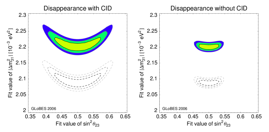
Figure 1: Comparison of $\Delta m_{31}^{2}$-$\theta_{23}$-precision between CID (left) and no CID (right) in the disappearance channel including all correlations ($1\sigma$, $2\sigma$, $3\sigma$, 2 d.o.f., $\sin^{2}2\theta_{13}=0$). The appearance information is added as usual with CID. Dashed curves correspond to the inverted hierarchy solution.

Compared to the NuFact-II setup from Ref. [20], we split the raw dataset into two samples: One with charge identification (CID), the other without, where the dataset with charge identification is used for the appearance channel and modeled according to Ref. [20]. As it can be seen from Figure 1, it turns out to be useful not to use the CID information for the disappearance channels (cf., Ref. [26]). This allows to use also the low energy bins with full efficiency, which maximizes the oscillatory signal. The price one has to pay for that is that the neutrino and antineutrino rates have to be added in this case, which is not a major problem for the disappearance channel [23]. However, as pointed out in Ref. [26], the higher event rates at low energies may lead to relatively fast oscillations especially for long baselines, which can lead to problems for large muon energies and small bin numbers. Therefore, we change the binning and use $43$ bins in total. In addition, we use the filter feature from GLoBES in order to average any fast oscillations already on the probability level over a width of $150\,\mathrm{MeV}$. We have tested that this choice appropriately describes the low energy range where the first significant events enter in order to allow muon energies up to about $100\,\mathrm{GeV}$ in combination with baselines up to about $9\,000\,\mathrm{km}$. Since we do not use CID in the disappearance channel, we use the MINOS efficiencies and threshold from Refs. [8, 65] in this channel. Note that we now have two different energy threshold functions. The fact that there are almost no events below about $4\,\mathrm{GeV}$ in the appearance channel is appropriately modeled. Finally, we choose 2.5% for the signal normalization errors, 20% for the background normalization errors, and $\sigma_{E}=0.15\,E_{\nu}$ for the energy resolution.

3.2 Optimized reach in $\boldsymbol{\sin^{2}2\theta_{13}}$ as function of energy and baseline

We now discuss the optimization of $L$ and $E_{\mu}$ for the $\sin^{2}2\theta_{13}$ sensitivity, CP violation sensitivity, and mass hierarchy sensitivity, assuming that we have a single “standard” neutrino factory experiment. In this section, we are mainly interested in the reach in $\sin^{2}2\theta_{13}$, i.e., the smallest values of $\sin^{2}2\theta_{13}$ for which a given performance indicator can be probed.

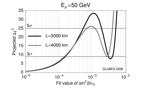
Figure 2: Projected $\Delta\chi^{2}$ for the $\sin^{2}2\theta_{13}$ sensitivity as function of the fit value of $\sin^{2}2\theta_{13}$ for $E_{\mu}=50\,\mathrm{GeV}$ and two different baselines as given in the plot legend (includes degeneracies).

For the $\sin^{2}2\theta_{13}$ sensitivity, one has to be carful to interpret the results with respect to the $(\theta_{13},\delta_{\mathrm{CP}})$-degeneracy [18]. We illustrate this challenge in Figure 2. Since we define the $\sin^{2}2\theta_{13}$ sensitivity as the largest $\sin^{2}2\theta_{13}$ which fits $\sin^{2}2\theta_{13}=0$, any degenerate solution will destroy the $\sin^{2}2\theta_{13}$ sensitivity. The interpretation in terms of the $(\theta_{13},\delta_{\mathrm{CP}})$-degeneracy is then as follows: If there is no signal (hypothesis $\sin^{2}2\theta_{13}=0$), this degeneracy (see bumps in the right-hand side of the figure) will destroy the $\sin^{2}2\theta_{13}$ sensitivity, i.e., a fake solution with a relatively large $\sin^{2}2\theta_{13}$ will still be consistent with $\sin^{2}2\theta_{13}=0$. Therefore, one will not be able to exclude that $\sin^{2}2\theta_{13}$ could be rather large. Since we want the results to be robust with respect to this definition, we choose $\Delta\chi^{2}=25$ (corresponding to $5\sigma$) for all $\sin^{2}2\theta_{13}$ sensitivity plots. As one can read off from Figure 2, choosing the $\Delta\chi^{2}=9$ (corresponding to $3\sigma$) would imply that very small changes in luminosity and configuration could, depending on the baseline, lead to jumps of the $\sin^{2}2\theta_{13}$ sensitivity by an order of magnitude. For example, if one was not able to achieve the originally anticipated luminosity by 10% for $\Delta\chi^{2}=9$, the results would look qualitatively different. However, for $\Delta\chi^{2}=25$, the degeneracy will always be visible in the two different baseline cases in Figure 2, and these two cases will be interpreted as qualitatively similar (which they in fact are).

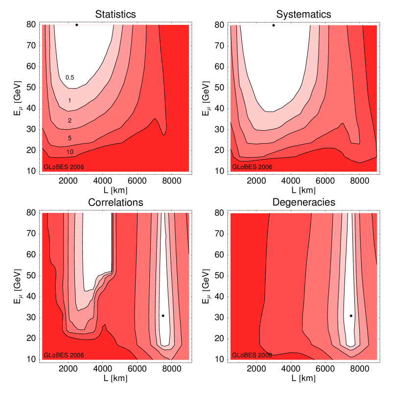
Figure 3: Sensitivity to $\sin^{2}2\theta_{13}$ ($5\sigma$) relative to the optimum (white) within each plot. The different panels correspond to successively taking into account statistics, systematics, correlations, and degeneracies. The different contours represent the region within a factor of 0.5, 1, 2, 5, and 10 above the optimal sensitivity in each plot. The optimal sensitivities are $\sin^{2}2\theta_{13}<1.4\cdot 10^{-5}$ (statistics), $2.8\cdot 10^{-5}$ (systematics), $2.4\cdot 10^{-4}$ (correlations), and $5.0\cdot 10^{-4}$ (degeneracies), obtained at the energies and baselines marked by the diamonds.

In Figure 3, we show the $\sin^{2}2\theta_{13}$ sensitivity ($5\sigma$) relative to the optimum (white) within each plot, i.e., the absolute minima in the different plots are different. Not surprisingly, for the systematics and correlations limits, baselines from $1\,000$ to $4\,000\,\mathrm{km}$ with as much muon energy as possible give the best sensitivities. However, including correlations and degeneracies, the “magic baseline” [55] at about $7\,500\,\mathrm{km}$ becomes more emphasized, where a correlation- and degeneracy-free measurement of $\sin^{2}2\theta_{13}$ is possible. Most importantly, the optimal muon energies do not need to be higher than about $40\,\mathrm{GeV}$, even $30\,\mathrm{GeV}$ are absolutely sufficient for the long baseline. The reason for this is that the $\sin^{2}2\theta_{13}$-term in the appearance probability does not drop as function of baseline at the mantle matter resonance energy. Therefore, matter effects prefer lower energies, whereas higher muon energies imply higher event rates and a relative decrease of events at the mantle resonance. The optimum is determined by a balance between these two factors. We have compared these results with the $\sin^{2}2\theta_{13}$ discovery reach (systematics only). We find that qualitatively the $\sin^{2}2\theta_{13}$ discovery reach for a CP fraction of $0$ (best case of $\delta_{\mathrm{CP}}$) is very similar to the upper row of Figure 3, but the $\sin^{2}2\theta_{13}$ discovery reach for a CP fraction of $100\%$ (conservative $\delta_{\mathrm{CP}}$) corresponds more to the lower row of Figure 3. This result is not very surprising, since the $\sin^{2}2\theta_{13}$ sensitivity basically corresponds to the conservative, i.e. worst case true value of $\delta_{\mathrm{CP}}$, discovery reach.

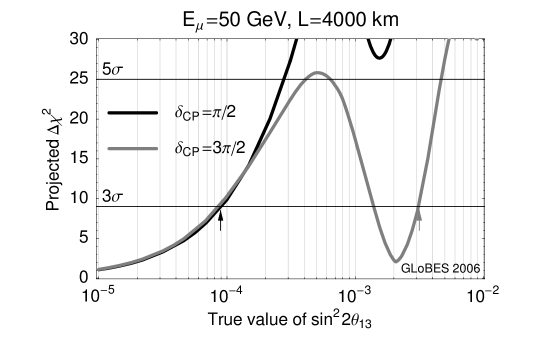
Figure 4: Projected (marginalized) $\Delta\chi^{2}$ for the sensitivities to maximal CP violation $\delta_{\mathrm{CP}}=\pi/2$ and $\delta_{\mathrm{CP}}=3\pi/2$ as function of the true value of $\sin^{2}2\theta_{13}$ for $E_{\mu}=50\,\mathrm{GeV}$ and $L=4\,000\,\mathrm{km}$. Sensitivity to maximal CP violation is given where $\Delta\chi^{2}>9$ ($3\sigma$). The arrow represents the “conservative” reaches for $\delta_{\mathrm{CP}}=\pi/2$ (gray arrow) and $\delta_{\mathrm{CP}}=3\pi/2$ (black arrow) used for Figure 5, i.e., thresholds in $\sin^{2}2\theta_{13}$ above which CP violation can be found for any value of $\sin^{2}2\theta_{13}$.

In order to discuss the CP violation sensitivity in terms of the $L$-$E$-optimization, we have to sufficiently condense the information. Since we are interested in the $\sin^{2}2\theta_{13}$ reach, i.e., the smallest values of $\sin^{2}2\theta_{13}$ for which one can measure leptonic CP violation, we have to define how to deal with “gaps” in the $\sin^{2}2\theta_{13}$ direction. This is illustrated in Figure 4, where CP violation sensitivity is given for all shown true values of $\sin^{2}2\theta_{13}$ when the function is above the chosen confidence level line. Obviously, for maximal CP violation $\delta_{\mathrm{CP}}=3\pi/2$, there is a gap independent of the choice of $\Delta\chi^{2}=9$ or $25$, which is not present for $\delta_{\mathrm{CP}}=\pi/2$. Therefore, we choose $\Delta\chi^{2}=9$ for all mass hierarchy and CP violation measurements because the qualitative interpretation hardly depends on the confidence level. In order to determine the $\sin^{2}2\theta_{13}$ reach, we choose the rightmost intersection with the chosen CL line, as illustrated by the arrows for the two different curves (“conservative reach”). In order to illustrate the details for CP violation and mass hierarchy we will show both figures with compressed information as well as we will later show all regions where these measurements are possible. Note that the interpretation is very different from the $\sin^{2}2\theta_{13}$ sensitivity: Since we show the CP violation sensitivity as function of the true $\sin^{2}2\theta_{13}$, we are, in principle, interested in all regions of the parameter space where we can measure leptonic CP violation. This means that one can measure CP violation if nature has chosen a value in the sensitive regions. If there is only a small gap, not finding CP violation in some sense would be “bad luck”. On the other hand it is a real risk for the experiment to fail. For the $\sin^{2}2\theta_{13}$ sensitivity, however, such a gap in the fitted value of $\sin^{2}2\theta_{13}$ would mean that we could not establish a small exclusion limit.

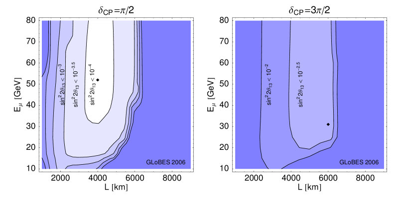
Figure 5: Sensitivity to maximal CP violation ($\delta_{\mathrm{CP}}=\pi/2$ or $3\pi/2$) for a normal mass hierarchy as function of $L$ and $E$. The sensitivity is given as absolute reach in $\sin^{2}2\theta_{13}$ at the $3\sigma$ confidence level including all parameter correlations and degeneracies. The minima are at $\sin^{2}2\theta_{13}=8.8\cdot 10^{-5}$ (left plot) and $\sin^{2}2\theta_{13}=1.3\cdot 10^{-3}$ (right plot) and marked by the diamonds. See text for more explanations and definition of the $\sin^{2}2\theta_{13}$ reach.

We show in Figure 5 the sensitivity to maximal CP violation for the two different choices of $\delta_{\mathrm{CP}}$. For $\delta_{\mathrm{CP}}=\pi/2$, we find the optimal performance at about $3\,000-5\,000\,\mathrm{km}$ for $E_{\mu}\gtrsim 30\,\mathrm{GeV}$, where large energies are not necessary. For the case $\delta_{\mathrm{CP}}=3\pi/2$, the absolute $\sin^{2}2\theta_{13}$ reach is rather poor, where we again have in this case shown the most conservative value of $\sin^{2}2\theta_{13}$ above which CP violation can be determined. In this case, degeneracies affect the CP violation performance. As it has been demonstrated in Ref. [21], the “magic baseline” can be used to resolve these degeneracies in the third and fourth quadrants of $\delta_{\mathrm{CP}}$. Therefore, in order to have optimal performance, a second baseline is necessary if $\delta_{\mathrm{CP}}$ turned out to be in this region.

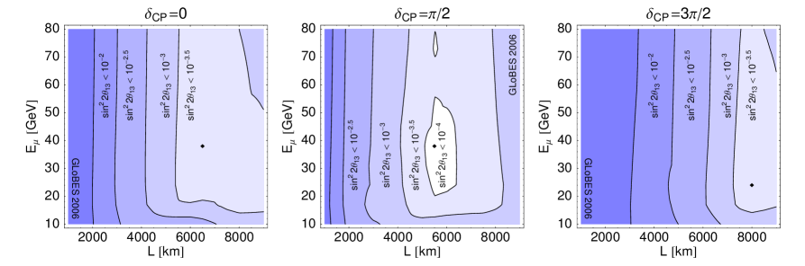
Figure 6: Sensitivity to a normal mass hierarchy for different values of $\delta_{\mathrm{CP}}$ (plot labels) as function of $L$ and $E$. The sensitivity is given as absolute reach in $\sin^{2}2\theta_{13}$ at the $3\sigma$ confidence level including all parameter correlations and degeneracies. The minima are at $\sin^{2}2\theta_{13}=1.8\cdot 10^{-4}$ (left plot), $\sin^{2}2\theta_{13}=6.7\cdot 10^{-5}$ (middle plot), and $\sin^{2}2\theta_{13}=1.6\cdot 10^{-4}$ (right plot) and marked by the diamonds. See text for more explanations and definition of the $\sin^{2}2\theta_{13}$ reach.

The normal mass hierarchy sensitivity reach in $\sin^{2}2\theta_{13}$ is shown in Figure 6 for different values of $\delta_{\mathrm{CP}}$. As one can read off this figure, the mass hierarchy sensitivity essentially increases with the baseline because of matter effects. This means that for very small true values of $\sin^{2}2\theta_{13}$, one will need a very long baseline. The muon energy is of secondary interest, as long as it is larger than about $20\,\mathrm{GeV}$. In fact, for $\delta_{\mathrm{CP}}=\pi/2$ or very long baselines $L>8\,000\,\mathrm{km}$, having a muon energy larger than $50\,\mathrm{GeV}$ is unfavorable because of the matter resonance at lower energies. In all cases, the “magic baseline” $L\simeq 7\,500\,\mathrm{km}$ is near the optimum. There is, however, one feature which is not shown in Figure 6: For certain values of $\delta_{\mathrm{CP}}$, there are gaps in the $\sin^{2}2\theta_{13}$ direction (similar to Figure 4). In Figure 6, such gaps occur for $\delta_{\mathrm{CP}}=3\pi/2$, and we have chosen to show the most conservative value of $\sin^{2}2\theta_{13}$ above which mass hierarchy sensitivity can be achieved for all values of $\sin^{2}2\theta_{13}$. Therefore, Figure 6, right, actually shows the ranges for the “gap-less” determination of the mass hierarchy. Thus, for very long baselines $L\gtrsim 7\,500\,\mathrm{km}$, the mass hierarchy can be determined in the full shown range of $\sin^{2}2\theta_{13}$. Note that in this case such a baseline itself allows to resolve the degeneracies.

As far as the dependence on the true $\Delta m_{31}^{2}$ is concerned, we have tested somewhat larger values of $\Delta m_{31}^{2}$, which could be suggested by the latest MINOS results [66], for the $\sin^{2}2\theta_{13}$ and CP violation sensitivities. For the $\sin^{2}2\theta_{13}$ sensitivity, the “magic baseline” choice does not depend on $\Delta m_{31}^{2}$. However, for $\Delta m_{31}^{2}$ somewhat larger than the current best-fit value, the rates at both the short and long baseline choices increase, and so does the absolute performance at both baselines. However, it turns out that the relative improvement at the magic baseline is even stronger, i.e., this baseline choice becomes even more emphasized. For CP violation, the effect of a larger $\Delta m_{31}^{2}$ is essentially an improvement of the absolute reach without baseline re-optimization (but slightly larger values of $E_{\mu}\gtrsim 40\,\mathrm{GeV}$ preferred). In addition, the baseline window where one can measure CP violation becomes slightly broader. For the mass hierarchy sensitivity, the absolute baseline length determines the $\sin^{2}2\theta_{13}$ reach, which means that the optimization should hardly depend on $\Delta m_{31}^{2}$.

3.3 Optimized precision of the leading atmospheric parameters

Except from any suppressed three-flavor effects, a neutrino factory might be useful for the precision measurement of the leading atmospheric parameters $\Delta m_{31}^{2}$ and $\theta_{23}$. For simplicity, we discuss the case of the true $\sin^{2}2\theta_{13}=0$ in this section, because $\sin^{2}2\theta_{13}>0$ yields complicated correlations in the disappearance channel (cf., Eq. (33) in Ref. [51]). In addition, we do not include degeneracies for the $\Delta m_{31}^{2}$ precision. For $\theta_{23}$, we are mainly interested in deviations from maximal mixing, which turns out to be a useful indicator for neutrino mass models [67]. Of course, this indicator is only useful if $\theta_{23}$ is consistent with maximal mixing before the neutrino factory operation. However, the precision of $\theta_{23}$ behaves very similar.

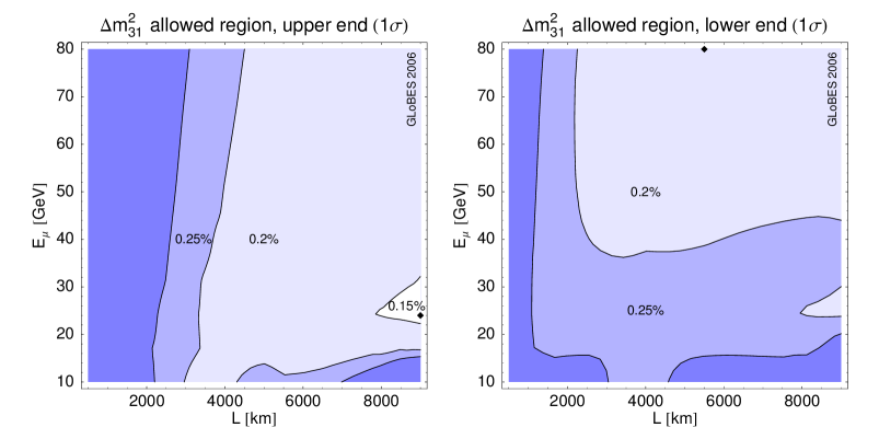
Figure 7: Precision of $\Delta m_{31}^{2}$ for a normal mass hierarchy and $\sin^{2}2\theta_{13}=0$ as function of $L$ and $E$. The precision is given as relative precision $\Delta m_{31}^{2}$ in per cent at the $1\sigma$ confidence level including all parameter correlations. The upper end (left panel) and lower end (right panel) of the allowed region are given separately because the $\Delta\chi^{2}$ is quite asymmetric. The minima occur at 0.14% (left) and 0.18% (right) and are marked by the diamonds.

We show in Figure 7 the precision of $\Delta m_{31}^{2}$ for a normal mass hierarchy and $\sin^{2}2\theta_{13}=0$ as function of $L$ and $E$. The precision is given as relative precision $\Delta m_{31}^{2}$ in per cent at the $1\sigma$ confidence level including all parameter correlations. The upper end (left panel) and lower end (right panel) of the allowed region are given separately, because the $\Delta\chi^{2}$ is quite asymmetric in many cases. As the most important result, the separate analysis of the dataset without CID yields an extremely good relative precision of $\Delta m_{31}^{2}$ of the order of $0.2\%$ for $L\gtrsim 3\,000\,\mathrm{km}$ and $E_{\mu}\gtrsim 40\,\mathrm{GeV}$. This extremely high precision comes, compared to Ref. [19], from the ability to resolve the oscillation maximum at low energies for long enough baselines and good enough statistics because of the improved threshold function without CID. In addition, the overall efficiency of the disappearance channel is higher without CID. Though the total rate decreases for longer baselines, more oscillation maxima can be resolved. Note that we have included sufficiently many bins at low energies to incorporate these effects. In general, the first oscillation maximum can be found at

$$\frac{L_{\mathrm{max}}}{\mathrm{km}}\sim 564\,\frac{E}{\mathrm{GeV}}\,,$$ (11)

which more or less determines the optimal configuration. If $L\ll L_{\mathrm{max}}$, the $\sin$-term in the oscillation probability can be expanded and $\theta_{23}$ and $\Delta m_{31}^{2}$ are highly correlated. This means that $L\gtrsim 1\,000\,\mathrm{km}$ is a necessary condition to be able to disentangle $\theta_{23}$ from $\Delta m_{31}^{2}$ because of the energies where the first significant events enter ($\sim 2\,\mathrm{GeV}$). In addition, this formula explains the optimum for $E_{\mu}\sim 10\,\mathrm{GeV}$ at about $3\ 500\,\mathrm{km}$ if one takes into account that the mean energy is somewhat below $E_{\mu}$. In summary, a neutrino factory optimized for $\Delta m_{31}^{2}$ has an very good precision compared to all other available technologies.

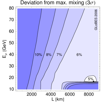
Figure 8: Sensitivity to deviations from maximal mixing for a normal mass hierarchy and $\sin^{2}2\theta_{13}=0$ as function of $L$ and $E$. The sensitivity is given as relative deviation of $\sin^{2}\theta_{23}$ from $0.5$ in per cent at the $3\sigma$ confidence level including all parameter correlations, where only the upper branch $\sin^{2}\theta_{23}>0.5$ is taken into account. The minimum as at 4.2% and marked by the diamond.

For $\theta_{23}$, we show in Figure 8 the sensitivity to deviations from maximal mixing for a normal mass hierarchy and $\sin^{2}2\theta_{13}=0$ as function of $L$ and $E$. The sensitivity is given as relative deviation of $\sin^{2}\theta_{23}$ from $0.5$ in per cent at the $3\sigma$ confidence level including all parameter correlations. Note that only the upper branch $\sin^{2}\theta_{23}>0.5$ is taken into account, because there is hardly any sensitivity to the $(\theta_{23},\pi/2-\theta_{23})$ ambiguity [54] and the problem is very symmetric around $\theta_{23}=\pi/4$. We find a very similar qualitative and quantitative behavior compared to Ref. [19]. However, the low energy performance for very long baselines $L\gtrsim 6\,000\,\mathrm{km}$ is significantly improved because the efficiencies at lower energies are better without CID. Most importantly, it is very hard to improve the sensitivity to deviations from maximal mixing with the given setup, probably because of the rather large normalization uncertainties. In particular, T2HK could achieve a similar quantitative performance [67].

3.4 Optimization for large $\boldsymbol{\sin^{2}2\theta_{13}}$

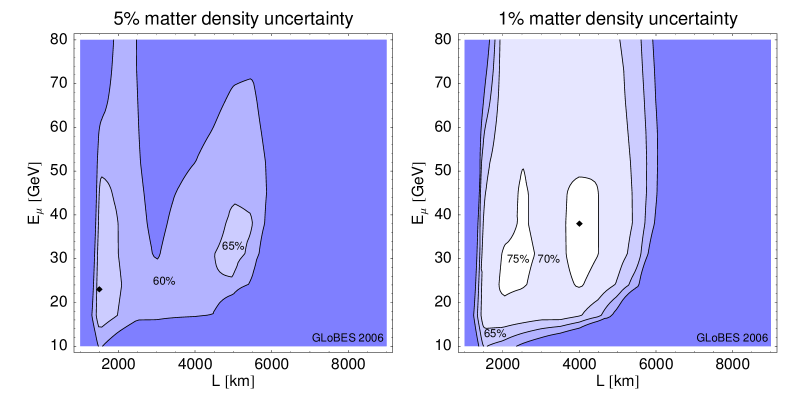
Figure 9: Fraction of (true) $\delta_{\mathrm{CP}}$ as function of $L$ and $E$ for the measurement of CP violation for $\sin^{2}2\theta_{13}=0.1$ and a normal mass hierarchy ($3\sigma$, including all parameter correlations and degeneracies). The left panel corresponds to a matter density uncertainty of $5\%$, and the right panel to a matter density uncertainty of $1\%$. The optima are at 68% (left plot) and 77% (right plot) and are marked by the diamonds.

Let us now assume that $\sin^{2}2\theta_{13}$ is large, such as $\sin^{2}2\theta_{13}\simeq 0.1$, which means that it will be quickly found by the next generation of superbeam experiments. However, it is well known that for large $\sin^{2}2\theta_{13}$ matter density uncertainties affect the precision measurements of $\sin^{2}2\theta_{13}$ and $\delta_{\mathrm{CP}}$ (see, e.g., Refs. [20, 64]). Therefore, it is an interesting question if the optimization changes for large $\sin^{2}2\theta_{13}$, and if one can exceed the performance of conventional techniques. Since maximal CP violation measurements and mass hierarchy measurements should for most parameter values not be a problem in this case, but usually depend on the true $\delta_{\mathrm{CP}}$, we choose as a performance indicator the fraction of all values of $\delta_{\mathrm{CP}}$ for which CP violation or the mass hierarchy can be established at the $3\sigma$ confidence level.

For the mass hierarchy, we find that the optimization is hardly affected by the matter density uncertainty. As a general rule of thumb, one can measure it for all values of $\delta_{\mathrm{CP}}$ for $L\gtrsim 1\,000\,\mathrm{km}$ almost independent of the muon energy. Later, we will also demonstrate that the discovery of $\sin^{2}2\theta_{13}$ is possible independent of $\sin^{2}2\theta_{13}$. This means that the only relevant question for large $\sin^{2}2\theta_{13}$ is the CP violation sensitivity, which we show in Figure 9 as the CP fraction for $\sin^{2}2\theta_{13}=0.1$ and a normal mass hierarchy as function of $L$ and $E$. The left panel corresponds to a matter density uncertainty of $5\%$, and the right panel to a matter density uncertainty of $1\%$. As a first result, the maximum achievable CP fraction depends on the matter density uncertainty, and is only marginally affected by a different baseline choice in the window between $1\,500$ and $5\,500\,\mathrm{km}$ for small matter density uncertainties. Comparing Figure 9, right, with Figure 5, left, also illustrates that for small values of the matter density uncertainty, the “usual” optimization for CP violation is qualitatively recovered. However, from Figure 9, left, we can read off a very different result for large matter density uncertainties which are more realistic for current knowledge [63, 64, 68]. As a very important result, the often used combination $L=3\,000\,\mathrm{km}$, $E_{\mu}=50\,\mathrm{GeV}$ performs especially bad. It is not trivial to explain this minimum: First of all, small muon energies are preferred because matter density uncertainties hardly affect the the $\sin^{2}2\theta_{13}$-term in Eq. (2) (which is acting as background to the $\delta_{\mathrm{CP}}$ measurement) close to the matter resonance (cf., Figure 3 of Ref. [64]). Second, small baselines are preferred because there the matter effects are small in general, and therefore also the absolute impact of matter density uncertainties is small. Third, there is a second optimum for $L\simeq 5\,000\,\mathrm{km}$, where the CP asymmetric term is enhanced for $E\sim 10\,\mathrm{GeV}$ (cf., Eq. (11); remember that the mean energy of the spectrum is considerably below the muon energy). These factors together cause the structure in Figure 9, left. From Figure 9, right, we can read off that the optimal performance for small matter density uncertainties is reached in a wide range of $L$ and $E_{\mu}$.

Performance indicator	$L$ [km]	$E_{\mu}$ [GeV]
Three-flavor effects:
$\sin^{2}2\theta_{13}$ sensitivity	$\sim 7\,500$ (“magic baseline”)	20-50
Mass hierarchy sensitivity	$\gtrsim 6\,000$	20-50
Max. CP violation sensitivity	$\sim 3\,000-5\,000$	$>$ 30
Leading atmospheric parameters:
$\Delta m_{31}^{2}$ precision	$\gtrsim 3\,000$	$\gtrsim 40$
Deviation from maximal mixing ($\theta_{23}$)	$\gtrsim 3\,500+50\cdot E_{\mu}/\mathrm{GeV}$	$\gtrsim 20$
Optimization for large $\boldsymbol{\sin^{2}2\theta_{13}}$:
Mass hierarchy sensitivity	$>1\,000$	$>10$
CP violation sensitivity ($\Delta\rho=1\%\,\bar{\rho}$)	$\sim 1\,500-5\,500$	20-50
CP violation sensitivity ($\Delta\rho=5\%\,\bar{\rho}$)	$\sim 1\,500-2\,000$	20-50
	$\sim 4\,500-5\,500$	20-40

Table 1: Requirements for the near-optimal performance of our “standard neutrino factory” (one individual experiment) for $\Delta m_{31}^{2}=0.0022\,\mathrm{eV}^{2}$ for different performance indicators.

We summarize in Table 1 the requirements for the optimization of our standard neutrino factory. There are two very important results. For the baselines, we need two different baselines for the optimal performance: A “shorter” baseline $L\sim 3\,000-5\,000\,\mathrm{km}$ for CP violation and leading atmospheric parameter measurements, and a longer baseline $L\simeq 7\,500\,\mathrm{km}$ for the sensitivity to $\sin^{2}2\theta_{13}$, mass hierarchy sensitivity reach, and the disentanglement of degeneracies for CP violation measurements. For the muon energies, we find that $E_{\mu}\gtrsim 20\,\mathrm{GeV}$ is sufficient for most applications, and $E_{\mu}\sim 40\,\mathrm{GeV}$ should be on the safe side. Therefore, we find that the main challenge for a neutrino factory will be the baseline, which can affect the physics potential much more than a muon energy lower than previously assumed. For the rest of this work, we will consider two baselines for our standard neutrino factory, one at $4\,000\,\mathrm{km}$ right at the optimal $\sin^{2}2\theta_{13}$ reach for CP violation (and close to the optimum for large $\sin^{2}2\theta_{13}$), and one at $7\,500\,\mathrm{km}$ (magic baseline). For the muon energy, we will use $50\,\mathrm{GeV}$, unless stated otherwise.

4 Detector requirements

A neutrino factory requires a large investment into accelerator R&D and infrastructure. Therefore, it is worth to consider an increased effort on the detector side of the experiment. The aspect of joint optimization of both accelerator and detector has so far been neglected, where the main problem is the lack of reliable performance predictions for large magnetic detectors. The goal of this section is not to prove the feasibility of certain detector properties or parameters, but to demonstrate the possible gain in physics reach if certain properties can be achieved. Therefore, the following statements or assumptions about the detector performance are not to be mistaken as a claim of feasibility, but should be understood as desirable improvements to be determined by extensive R&D. Nevertheless, we have tried to choose our assumptions not too far away from what seems to be possible [69]. We will, however, discuss how variations of our assumptions affect the physics results in some cases. Thus, the results may serve as guideline where to focus efforts in detector R&D, and will be indicative of the expected improvements as well. They should be interpreted as “optimization potential of the detector” rather than as “optimized detector”.

4.1 Improved detector assumptions

The main limitation of a neutrino factory compared to other advanced neutrino facilities comes from the fact the standard detector has a relatively high neutrino energy threshold (necessary for charge identification), which makes the first oscillation maximum basically inaccessible (cf., Ref. [70]). All measurements have therefore to be performed in the high energy tail of the oscillation probability off the oscillation maximum. In different words, a neutrino factory is optimized for high statistics in the appearance channel, not for operation at the oscillation maximum. This is the reason why it seems to be the experiment most affected by the eightfold degeneracy [52, 20]. A number of solutions to this degeneracies problem has been proposed, amongst them it has been studied what a better detector in terms of a better neutrino energy threshold could achieve [20]. We will pick up this starting point and discuss improvements in the detection threshold and energy resolution in this section.

The high neutrino energy threshold in Ref. [70] is the result from optimizing for the purest possible sample of wrong sign muons, which clearly puts the emphasis on events with a high energy muon. The lower the muon energy is, the higher the likelihood to mis-identify the muon charge or the nature of the event (CC vs NC) becomes. Thus the background increases with decreasing neutrino energy, since the average muon energy will decrease with the neutrino energy. The background fraction scales with the neutrino energy such as a power law with a spectral index around $-2$. Our background model assumes that whatever happens with the threshold will only affect events below the threshold, but not events above, i.e., there is only down-feeding of background but no up-feeding. The reason behind this assumption is that a mis-identified NC event always should have a reconstructed energy which is lower than the true energy, since there is missing energy in every NC event. In order to roughly match the total background obtained in Ref. [70], we use a background fraction $\beta E_{\nu}^{-2}$ with $\beta=10^{-3}$. Integrating this background fraction from $4\,\mathrm{GeV}$ to $50\,\mathrm{GeV}$ yields an average background fraction of $5\cdot 10^{-6}$. We assume this background fraction separately for the background from neutral currents and wrong sign muons.

Achieving a lower threshold probably requires a finer granularity of the detector, i.e., a higher sampling density in the calorimeter. This should at the same time improve the energy resolution of the detector. We use a parameterization $\sigma_{E}\,[\mathrm{GeV}]=\sigma\,\sqrt{E_{\nu}\,[\mathrm{GeV}]}+0.085\,\mathrm{GeV}$ with $\sigma=0.15$ for the energy resolution (as compared to $\sigma_{E}=0.15\,E_{\nu}$ before, corresponding to $\sigma\simeq 0.5$), where the constant part models a lower limit from Fermi motion. For definiteness, we take the neutrino energy threshold to be $1\,\mathrm{GeV}$, and the efficiency to be constant $0.5$ for all appearance neutrino events above threshold. This setup of combined lower threshold, increasing background fraction, and better energy resolution will be called “optimal appearance”. Similar numbers are quoted for the NO$\nu$A detector [71], which is a totally active calorimeter.

In order to illustrate the sensitivity of the results to these numbers, we will use the following setups:

1. Standard detector, as from the last section.

2. Optimal appearance: $\sigma=15\%$, $\beta=10^{-3}$, full efficiency of 50% already reached at $1\,\mathrm{GeV}$.

3. Better threshold: Same as 2), but $\sigma=50\%$ (similar to 1).

4. Better energy resolution: Same as 2), but old threshold from 1).

As before, we we assume that the systematical background uncertainty is $20\%$ and the corresponding error $s$ for the signal is $s=2.5\%$ for all these setups.

4.2 Impact on physics reach

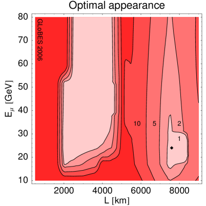
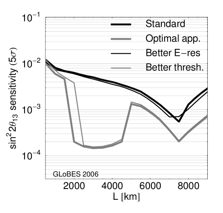
Figure 10: $\sin^{2}2\theta_{13}$ sensitivity ($5\sigma$) for several improved detector options. The left hand panel shows the $\sin^{2}2\theta_{13}$ sensitivity as function of baseline and muon energy relative to the minimum for the ‘optimal appearance’ detector including degeneracies similar to Figure 3 (lower right). The minimum appears at $\sin^{2}2\theta_{13}=1.1\cdot 10^{-4}$ marked by the diamond. The right hand panel shows the $\sin^{2}2\theta_{13}$ sensitivity as function of baseline for different detector options (see plot legend) and $E_{\mu}=50\,\mathrm{GeV}$ fixed. Note that the better energy resolution option uses a different background model, which leads to the crossing with the “standard” curve at $L\sim 7\,500\,\mathrm{km}$.

Changing the detector threshold by a large amount certainly should impact the choice of the optimal baseline and muon energy. In the left panel of Figure 10, the sensitivity to $\sin^{2}2\theta_{13}$ at $5\,\sigma$ is shown for the optimal detector as a function of the baseline and muon energy including degeneracies. The optimum is marked by the diamond and has a value of $\sin^{2}2\theta_{13}=1.1\cdot 10^{-4}$, it is located at around $7\,500\,\mathrm{km}$ and $E_{\mu}=24\,\mathrm{GeV}$ similar to Figure 3 (lower right). Compared to Figure 3, the second optimum at shorter baselines is still present including degeneracies, and the allowed muon energies tend to be rather low. Even energies as low as $20\,\mathrm{GeV}$ now work reasonably well for both baselines. Next is is interesting to see whether the improvements are mainly due to the lower threshold or energy resolution. This is illustrated in the right hand panel of Figure 10, where different combinations of better threshold or energy resolution are compared with the standard setup with respect to their $\sin^{2}2\theta_{13}$ sensitivity (in this figure, $E_{\mu}$ is fixed to $50\,\mathrm{GeV}$). The main effect for the $\sin^{2}2\theta_{13}$ sensitivity improvement clearly comes from lower energy threshold, the better energy resolution only plays a very minor role. Note that the optimum in this figure occurs at around $3\,000\,\mathrm{km}$ for the optimal detector because we have fixed the muon energy. A comparison to Figure 10, left, illustrates that this is not the global minimum in $L$-$E_{\mu}$-space.

The behavior for the other performance indicators CP violation and mass hierarchy is slightly different, as we discuss with Figure 11. In this figure, $\delta_{\mathrm{CP}}=3\pi/2$ was chosen since for this specific value degeneracies have a large impact (compared to $\delta_{\mathrm{CP}}=\pi/2$) and any improvements are most obvious there.

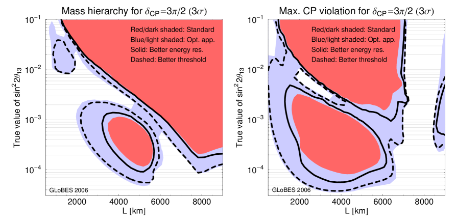
Figure 11: The normal mass hierarchy (left) and CP violation (right) sensitivities ($3\sigma$) as function of baseline and true $\sin^{2}2\theta_{13}$ for a normal hierarchy and $\delta_{\mathrm{CP}}=3\pi/2$, different detector options (see legend), and $E_{\mu}=50\,\mathrm{GeV}$. Sensitivity is given in the shaded/enclosed regions.

The left hand panel shows the sensitivity to the mass hierarchy at $3\,\sigma$, where sensitivity is given within the shaded/ marked areas. The red (dark) shaded regions shows the result for the standard detector whereas the blue (light) shaded region shows the result for the optimal setup. Clearly, the accessible range in $\sin^{2}2\theta_{13}$ improves as well as the constraints on the baseline become somewhat weaker for the better detector. The difference between having only a better threshold (dashed line) and only a better energy resolution (solid line) is quite large. Therefore, for the mass hierarchy the main improvement comes from to the lower threshold as well. For CP violation in the right panel of Figure 11, the detailed picture looks different but the conclusion is the same: Large improvements come from a lower threshold, and there is only minor influence of the energy resolution. The choice of the optimal $L$ and $E$ seems to be basically unaffected by a better detector.

One important issue in this context is the performance of a neutrino factory if $\sin^{2}2\theta_{13}$ turns out to large, such as around $0.1$. There will be information regarding this case from reactor experiments by around 2010, such as from Double Chooz [7, 72]. Note that we have stated earlier that $\sin^{2}2\theta_{13}$ discovery and mass hierarchy measurements are unproblematic for large values of $\sin^{2}2\theta_{13}$, which means that the optimization is determined by $\delta_{\mathrm{CP}}$ measurements. We show in Figure 12 the fraction of $\delta_{\mathrm{CP}}$ for the sensitivity to CP violation as a function of the baseline for $\sin^{2}2\theta_{13}=0.1$ and different combinations of experimental setup and matter density errors. In the case of large $\sin^{2}2\theta_{13}$, alternative technologies, such as superbeams, can be very competitive in their physics reach. Therefore, we show for comparison as the grey line the CP fraction for which T2HK^∗ would be sensitive to CP violation. In the left hand panel the results are shown for the canonical value for the matter density uncertainty of $5\%$. Clearly the standard neutrino factory setup does not perform better than the superbeam. The situation changes once better detectors are considered. The optimal setup defined previously would yield a significant improvement over the superbeam for nearly all choices of the baseline above $1500\,\mathrm{km}$. It also can be seen that the improvement comes from both the lower threshold and better energy resolution. In this scenario, the detector performance is crucial in making the case for a neutrino factory.

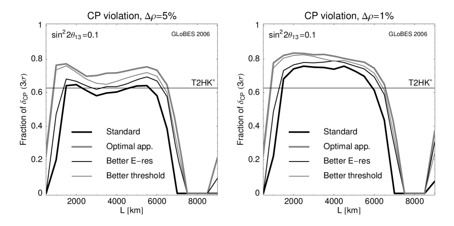
Figure 12: The CP fraction for the sensitivity to CP violation ($3\sigma$) for a normal hierarchy as function of baseline for different detector options (see legend) and $E_{\mu}=50\,\mathrm{GeV}$. The left plot correspond to $5\%$ matter density uncertainty, and the right plot to $1\%$ matter density uncertainty.

The right hand panel shows the result if the matter density uncertainty could be reduced down to $1\%$. Quite obviously this would further improve the performance of neutrino factory, as well as it affects the baseline somewhat. We have checked that these results for the optimal detector hold for a lower muon energies around $20\,\mathrm{GeV}$ as well, i.e., though $50\,\mathrm{GeV}$ do not harm, $20\,\mathrm{GeV}$ are sufficient in this case. Thus, for the case of large $\sin^{2}2\theta_{13}$, we conclude that improving the detector energy resolution and energy threshold would allow to choose a shorter baseline of about $1500\,\mathrm{km}$ and a muon energy of $20\,\mathrm{GeV}$, while the option $4000\,\mathrm{GeV}$ at $50\,\mathrm{km}$ does not mean a significant loss in sensitivity (the loss is, depending on the matter density uncertainty, about $0.05$ to $0.08$ in the CP fraction between the optimum and this point). Furthermore, for one neutrino factory baseline only, it can be concluded that lower threshold, better energy resolution, and lower matter density uncertainty would equally help to improve the performance.

4.3 Systematics impact and disappearance channel

Above we have defined a background model and assumed a certain systematical uncertainty on the signal. Here we show how our results for the measurement of CP violation change if we modify the input values for the background fraction $\beta$ and the signal normalization error $s$ (as defined in Section 4.1). In addition, we discuss the impact of energy resolution and systematics on the disappearance channel.

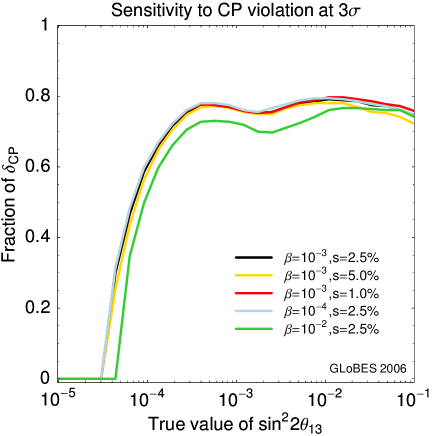
Figure 13: Fraction of $\delta_{\mathrm{CP}}$ for which CP violation can be established at $3\,\sigma$ as function of $\sin^{2}2\theta_{13}$. The different curves are for different assumptions about background and systematical uncertainty of the signal as defined in the legend.

Figure 13 shows the impact of varying the systematics parameters $\beta$ or $s$ on the CP violation measurement. To a very good approximation, it is safe to say that varying $s$ from $1\%$ to $5\%$ does not change the results at all. Furthermore, Figure 13 also shows that $\beta$ is only important as far as it may not become too large, but even a factor of 10 is not devastating. Note, that the error on the background is assumed to be $20\%$, which is quite conservative compared to the numbers usually quoted for superbeams. Certainly the impact of an increased background will be strongly reduced by reducing this uncertainty.

The disappearance channels are mainly used to determine the atmospheric neutrino parameters $\Delta m_{31}^{2}$ and $\sin^{2}\theta_{23}$. As shown in Figure 1, the obtainable accuracies are very impressive even with the standard setup. It also can be seen from that figure that having a low threshold is important in order to properly cover the first oscillation dip.

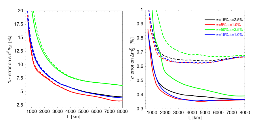
Figure 14: The relative $1\,\sigma$ (full width) errors on $\sin^{2}\theta_{23}$ (left hand panel) and $\Delta m_{31}^{2}$ (right hand panel) as a function of the baseline. The result is shown for various combinations of energy resolution $\sigma$ and systematic error $s$. The dashed lines assume an uncertainty on $\Delta m_{21}^{2}$ and $\theta_{12}$ of $10\%$, whereas the solid lines are calculated for the default value of $5\%$. The results are computed for $\sin^{2}2\theta_{13}\equiv 0$.

The optimal detector considered here will not improve the threshold for the disappearance channel (because we do not use charge identification for that channel), but the energy resolution will be much better. It has been demonstrated in Ref. [26] that the energy resolution has a large influence on the accuracy for the leading parameters. In Figure 14 the relative $1\,\sigma$ (full width) errors on $\sin^{2}\theta_{23}$ (left hand panel) and $\Delta m_{31}^{2}$ (right hand panel) as a function of the baseline are shown. The different colored lines correspond to different values of the energy resolution $\sigma$ and the normalization error of the signal $s$. Interestingly, the signal error $s$ seems to be quite unimportant. The energy resolution, on the other hand, has a relatively large impact, especially at the shorter baselines. The dashed lines show the results if the error on the solar parameters were $10\%$ instead of $5\%$, and one can see that this would deteriorate the results considerably. Irrespective of the error on the solar parameters and the energy resolution, longer baselines are preferred especially for $\sin^{2}\theta_{23}$.

5 Addition of silver and platinum channel data

So far we have discussed the $\nu_{\mu}\rightarrow\nu_{\mu}$-disappearance channel for the leading atmospheric oscillation parameters, and the “golden” $\nu_{e}\rightarrow\nu_{\mu}$-appearance channel for sub-leading three-flavor effects, i.e., $\sin^{2}2\theta_{13}$, $\delta_{\mathrm{CP}}$ and the sign of $\Delta m^{2}_{31}$. Besides these channels, the neutrino flavors contained in the beam of a neutrino factory allow for additional oscillation channels which could help to resolve correlations and degeneracies: the $\nu_{e}\rightarrow\nu_{\tau}$-appearance channel (“silver channel”) and the $\nu_{\mu}\rightarrow\nu_{e}$-appearance channel (“platinum channel”); for details on the phenomenology, see Section 2. In this section, we first describe the definition for the silver and platinum channels as is used throughout this work and discuss technical issues relevant for these channels as well. The silver channel has been studied in great detail in the context of the OPERA experiment and thus is very well understood in terms of the detector. For the platinum channel the situation is slightly less favorable since no reliable data on electron charge identification was available. For both additional channels, we define two setups, a standard scenario with a conservative choice of parameters and an optimistic scenario which certainly would require a considerable detector R&D effort to be realized. The idea is, to explore the possible maximal gain in physics reach which could be obtained by the optimistic setups in order to show whether an increased effort in R&D is necessary. For the silver channel, we also investigate optimization issues concerning the placement of the second detector. For both, we formulate the requirements to reach a certain level of improvement in the physics performance. Then, in the last subsection, we analyze the impact of this additional channel information for the three performance indicators introduced in Section 2 (the sensitivity limit to $\sin^{2}2\theta_{13}$, the sensitivity to maximal CP violation and the sensitivity to the sign of $\Delta m_{31}$), and we compare the different additional channels performances.

5.1 Silver channel

For the silver channel, the tau neutrinos are detected which are oscillating from the electron neutrinos in the beam. Since the neutrino energies at a neutrino factory are above the tau production threshold, tau leptons can be produced in charged-current reactions. The detection of these tau leptons from the $\nu_{e}\rightarrow\nu_{\tau}$ oscillation is called “silver channel” and was already discussed in the literature [56, 73]. The observation of the produced tau leptons is not possible at the “golden” detector, which means that a second Opera-like Emulsion Cloud Chamber (ECC) detector is assumed for the measurement. This kind of detector is capable of distinguishing the tau lepton events from other events by the observation of the decay topology of the tau decay. Our description of the silver channel follows Ref. [73]. The discussed OPERA-like ECC detector is capable of observing the decay of the charged-current produced tau leptons into muons. We incorporate an energy dependent threshold for the decay-produced muon identification. The evolution of this threshold was taken from Figure 7 in Ref. [73]. The energy resolution is assumed to be $20\%\times E$, which is also an optimistic choice. We assume silver channel data taking only during the $\mu^{+}$-stored phase.

Background source	Rejection factor
Neutrino induced charm production	$10^{-8}\,\times\,(N_{CC}(\nu_{e})+N_{CC}(\nu_{\mu}))$
Anti-neutrino induced charm production	$3.7\cdot 10^{-6}\,\times\,N_{CC}(\bar{\nu}_{\mu})$
$\tau^{+}\rightarrow\mu^{+}$ decays	$10^{-3}\,\times\,N_{CC}(\bar{\nu}_{\tau})$
$\mu$ matched to hadron track	$7\cdot 10^{-9}\,\times\,N_{CC}(\bar{\nu}_{\mu})$
Decay-in-flight and punch-trough hadrons	$6.97\cdot 10^{-7}\,\times N_{NC}\,+$
	$+\,2.1\cdot 10^{-8}\,\times\,N_{CC}(\nu_{e})$
Large-angle muon scattering	$10^{-8}\,\times\,N_{CC}(\nu_{\mu})$

Table 2: The background sources and rejection factors for the silver channel measurement in the $\mu^{+}$-stored phase. The numbers are taken from Ref. [73].

As indicated above, we define two setups representing the current “standard” assumptions and the improvement potential in the spirit of the last section for the golden detector:

• Standard: Silver
  We assume the ECC detector to have a fiducial mass of 5 kt as in Ref. [73]. In addition, we apply an overall signal efficiency of approximately 10%, which was chosen to reproduce the signal event numbers from Table 4 in Ref. [73]. The background rejection factors are taken from Ref. [73] as well, and are summarized in Table 2.

• Optimistic: Silver^∗
  In the standard scenario, it was assumed, that only leptonic tau decays can be observed. But, in principle, all the other decay channels of the tau lepton might be analyzed as well, this increases the signal by a factor of five. At the same time, we assume that those improvements necessary for identifying hadronic tau decays will allow to reduce the background somewhat and hence we take only three time the value of the standard setup [74]. Furthermore, we assume a fiducial detector mass of 10 kt.

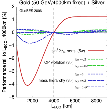
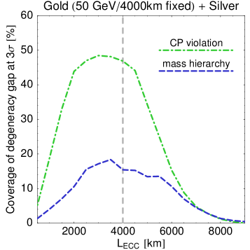
Figure 15: Optimization of the ECC detector baseline (standard silver channel scenario) for a fixed golden channel with $\mathrm{E_{\mu}=50\,GeV}$ and $\mathrm{L_{MID}=4000\,km}$. The ECC detector baseline is varied from 500 to 9000 km. Left-hand side (statistics dominated regime): The smallest $\sin^{2}2\theta_{13}$ for which sensitivity can be found for the three performance indicators $\sin^{2}2\theta_{13}$ sensitivity (solid red/dark curve), sensitivity to maximal CP violation (bright grey/green dashed curves), and sensitivity to normal mass hierarchy (dark grey/blue dashed curves) relative to the case of $\mathrm{L_{ECC}=L_{MID}=4000\,km}$ (negative numbers are better). Right-hand side (degeneracy resolution potential): The coverage of the sensitivity gap for sensitivity to maximal CP violation (dashed-dotted curve) and sensitivity to normal mass hierarchy (dashed curve), which appears for the golden channel alone for a medium $\sin^{2}2\theta_{13}\sim 10^{-2.5}$ and $\delta_{CP}=3\pi/2$ at 3$\sigma$. See text for details.

The silver channel detector can be operated independently from the golden channel detector, and can, in principle, be located at a different baseline. We checked that the additional silver channel data does not affect the golden channel baseline optimization. On the other hand, one can think of optimizing the silver baseline for a optimized fixed golden baseline of $\mathrm{L_{MID}=4000\,km}$, i.e., placing the silver channel detector at a different baseline. In Figure 15, the impact of a variation of the ECC detector baseline for the standard silver channel scenario is shown for the three performance indicators sensitivity to $\sin^{2}2\theta_{13}$, sensitivity to maximal CP violation, and sensitivity to normal mass hierarchy. There are two topics illustrated in this figure: On the left-hand side, we give the absolute reach in small $\sin^{2}2\theta_{13}$, i.e., the smallest true value of $\sin^{2}2\theta_{13}$ for which we still find sensitivity (statistics dominated regime). The absolute reach is shown relative to the $\mathrm{L_{ECC}=L_{MID}=4000\,km}$ case, where negative numbers refer to better performance. For CP violation and mass hierarchy sensitivity, the impact of the silver baseline variation is within less than 1%. The best sensitivity limit to $\sin^{2}2\theta_{13}$ is given at a ECC detector baseline of 1500 km, but also here, the effect is only 4% because of the low event rate for small $\sin^{2}2\theta_{13}$. Note that this effect would hardly be visible on a logarithmic scale, such as in Figure 11. A different topic is illustrated in Figure 15, right (degeneracy resolution potential): As easily visible in Figure 11, the golden channel measurement suffers significantly from degeneracies for true $\delta_{CP}=3\pi/2$ at the $4\,000\,\mathrm{km}$ baseline. Therefore, at medium true values of $\sin^{2}2\theta_{13}\sim 10^{-2.5}$, the sensitivities to maximal CP violation and the normal mass hierarchy are lost, and a sensitivity gap appears. On the right-hand side of Figure 15 the coverage of this sensitivity gap is shown for the inclusion of silver channel data with varied ECC detector baselines. The gap is defined as the size of the region without sensitivity at $3\,\sigma$ in units of $\log\sin^{2}2\theta_{13}$. The golden channel is again fixed to an optimized setup with $\mathrm{E_{\mu}=50\,GeV}$ and $\mathrm{L_{MID}=4000\,km}$. As can be seen, the optimal ECC baselines to cover the sensitivity gap as much as possible is found between 2500 and 5000 km. This effect is visible on logarithmic scales of $\sin^{2}2\theta_{13}$, since we define the coverage width of the gap on a logarithmic scale. Because of this effect and because it is more cost effective, we will therefore assume in the following that the ECC detector be located at the golden main detector baseline.

5.2 Platinum channel

Background source	Rejection factor
Muon disappearance	$10^{-3}\,\times\,N_{CC}(\nu_{\mu})\,(N_{CC}(\bar{\nu}_{\mu}))$
Tau appearance	$5\cdot 10^{-2}\,\times\,N_{CC}(\nu_{\tau})\,(N_{CC}(\bar{\nu}_{\tau}))$
Neutral current reactions	$10^{-2}\,\times\,N_{NC}$
Wrong sign electron/positron	$10^{-2}\,\times\,N_{CC}(\bar{\nu}_{e})\,(N_{CC}(\nu_{e}))$

Table 3: The background sources and rejection factors for the platinum channel measurement for the $\mu^{-}$-stored phase, while the brackets refer to the $\mu^{+}$-stored phase. The numbers, besides the background from electron/positron CID, are taken from Ref. [75].

Besides the previously considered channels, the neutrino beam of a neutrino factory allows to observe neutrino oscillations from the $\nu_{\mu}/\bar{\nu}_{\mu}\rightarrow\nu_{e}/\bar{\nu}_{e}$ channel, which is often called “platinum channel”. This is the T-conjugated oscillation channel to the golden channel, and corresponds to the CP-conjugated golden channel with different matter effect. Therefore, it should allow to resolve the correlations and degeneracies of the golden channel measurements as well. Again, as for the silver channel, we define two different scenarios, one conservative and one optimistic. For the description of the platinum channel, we roughly follow the $\nu_{e}$-appearance performance of the MINOS detector, which has been estimated in Ref. [75]. However, since we require charge identification to establish the $\nu_{e}$ ($\bar{\nu}_{e}$) appearance against the $\bar{\nu}_{e}$ ($\nu_{e}$) disappearance from the beam, we add an extra background from these disappearance neutrinos. We assume the background after the CID selection to be 1% of all electron neutrino disappearance neutrinos. We apply a lower energy detection threshold at 0.5 GeV. Electron charge ID so far has been only studied for a magnetized liquid Argon TPC and the numbers above roughly match the ones indicated in [76]. In the same Ref. it was also pointed out that electron charge ID may have an upper threshold beyond which it may no longer be possible to measure the charge. Electrons/positrons at higher energies tend to shower early, which means that the track is too short and the curvature is hardly measurable. Therefore, the CID of electrons and positrons most likely is only possible up to a certain energy threshold.

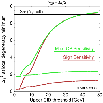
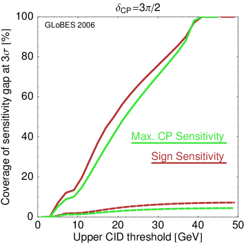
Figure 16: The evolution of the height of the $\Delta\chi^{2}$ at the local degeneracy minimum (left) and the coverage of the sensitivity gap (right) as function of the upper electron/positron CID threshold for the sensitivity to CP violation. The sensitivity gap (see Figure 15) and local degeneracy appear for about the true $\sin^{2}2\theta_{13}\approx 2.5\times 10^{-3}$ if the true value $\delta_{\mathrm{CP}}=3\pi/2$ is assumed. The different curves refer to the sensitivity to maximal CP violation (light gray/green) and sensitivity to the normal mass hierarchy (dark grey/red). The baseline is assumed to be 4000 km and the energy of the parent muons is 50 GeV. The dashed curves refer to the standard scenario with a lower detector mass (15 kt instead of 50 kt) and lower efficiencies (20% instead of 40%).

For the platinum channel, we will always assume the same baseline as for the golden channel, since it is at least in principle conceivable to use the same detector for both golden and platinum channel. We define two setups:

• Standard: Platinum
  We assume a platinum channel detector with a fiducial mass of 15 kt, which may be the largest magnetizable volume for a liquid argon TPC. The signal efficiency is taken to be 20% [76], and the background rejection factors are summarized in Table 3. Furthermore, the energy resolution is assumed to be $15\%\times E$. The upper threshold for the electron/positron CID is assumed to be 7.5 GeV. The CID background is assumed to be $1\%$ [76] and the other backgrounds are taken from Ref. [75].

• Optimistic: Platinum^∗
  We assume a platinum channel detector with a fiducial mass of 50 kt. This choice is inspired by the possibility (at least in principle) to use the same, improved detector than for the golden channel. The signal efficiency is 40%. The background rejection factors of Ref. [75] are extrapolated to higher energies. The CID background is the same than for the standard setup. Electron/positron CID is assumed to be possible to the highest energies and no upper threshold is imposed.

First,we will discuss the impact of the upper CID threshold and discuss the performance of the additional platinum channel data depending on the value of this threshold energy. Again, as the first case, we want to use the additional channel data to resolve the degeneracies, which especially appear for the choice of true $\delta_{\mathrm{CP}}=3\pi/2$. As indicated in Figure 4, the sensitivity gap for maximal CP violation appears as a local minimum in the projected $\Delta\chi^{2}$ at higher values of true $\sin^{2}2\theta_{13}$, which is also true for the mass hierarchy. In the left-hand side of Figure 16, we therefore show the height of these minima as function of the assumed upper electron/positron CID threshold for the platinum channel. One can easily see that the platinum channel data can help to resolve the degeneracy and push the minimum above the $3\sigma$ confidence level similar to the silver channel. However, it could only significantly contribute, if the CID were possible up to high energies larger than about 20 to 30 GeV. On the right-hand side of Figure 16, we show how the width of the sensitivity gap (already discussed in Figure 15) at $3\sigma$ evolves. For high CID thresholds, it can be covered completely. The dashed curves show the same results but for the reduced detector mass and efficiencies. One can see, that in this case, the reduced statistics in the platinum channel data cannot help to resolve the degeneracy. In order to show the maximal contribution from platinum data and its usefulness for the physics performance, we will only discuss platinum CID thresholds possible up to $50\,\mathrm{GeV}$.

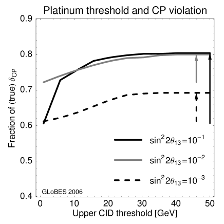
Figure 17: The fraction of (true) $\delta_{\mathrm{CP}}$ for which CP violation can be discovered at the $3\sigma$ confidence level as function of the upper platinum CID threshold (for a normal mass hierarchy). As a setup, we use the golden and platinum channels (platinum with 50 kt mass, 40% detection efficiency) at $4\,000\,\mathrm{km}$ for $E_{\mu}=50\,\mathrm{GeV}$. The different curves correspond to different values of $\sin^{2}2\theta_{13}$ as given in the plot legend. The arrows refer to the improvement in the physics potential by using the platinum channel.

As opposed to using the platinum channel to resolve degeneracies for medium $\sin^{2}2\theta_{13}$, we will also discuss its potential for large $\sin^{2}2\theta_{13}$. We show in Figure 17 the fraction of (true) $\delta_{\mathrm{CP}}$ for which CP violation can be discovered as function of the upper platinum CID threshold, i.e., we discuss the performance for all values of $\delta_{\mathrm{CP}}$ in this figure. As in Figure 16, one can easily see the relatively shallow dependence on the threshold for $\sin^{2}2\theta_{13}\lesssim 10^{-2}$, whereas for large $\sin^{2}2\theta_{13}$ already a $6\,\mathrm{GeV}$ upper threshold can increase the fraction of $\delta_{\mathrm{CP}}$ by about 10%. This means that if it turns out that the platinum channel is mainly useful for large $\sin^{2}2\theta_{13}$, a relatively low upper threshold will not harm. However, if we intend to use it for medium $\sin^{2}2\theta_{13}$ as a degeneracy resolver, the threshold will need to be as high as 20 to 30 GeV.

Configuration	Fraction of $\delta_{\mathrm{CP}}$
Golden only	61%
Golden+$\nu_{e}$/$\bar{\nu_{e}}$-disappearance (with CID)	71%
Golden+$\nu_{e}$/$\bar{\nu_{e}}$-disappearance (without CID)	76%
Golden+Platinum∗ ($\nu_{e}$/$\bar{\nu_{e}}$-appearance)	80%
Golden+Platinum∗+$\nu_{e}$/$\bar{\nu_{e}}$-disappearance (with CID)	82%

Table 4: The fraction of (true) $\delta_{\mathrm{CP}}$ in per cent for which CP violation can be discovered for $\sin^{2}2\theta_{13}=0.1$ and a normal mass hierarchy for several electron neutrino detection options. For the detector parameters (efficiencies, etc.), the same values as for the Platinum^∗ channel have been used. For the option without CID, we have added the electron neutrino appearance and disappearance signals. For all options, a 2.5% normalization error has been used, but we have checked that the results do not change for a 1% normalization error.

While we have only considered electron neutrino (and anti-neutrino) appearance in this section, one could also think about implementing the electron neutrino disappearance channels. We have tested the impact of these channels for $\sin^{2}2\theta_{13}=0.1$ (where the effect on the disappearance is largest), and we have found some improvement for large $\sin^{2}2\theta_{13}$, which is, however, not as good as the platinum appearance potential. We show in Table 4 several options with electron neutrino detection for large $\sin^{2}2\theta_{13}=0.1$. Obviously, for the platinum channel with CID the best potential can be achieved, and an additional 2% in the fraction of $\delta_{\mathrm{CP}}$ can be gained by using the $\nu_{e}$/$\bar{\nu_{e}}$-disappearance channels as well. However, if one cannot achieve CID to the anticipated level/upper energies, the disappearance channel alone without CID can also provide some additional information. Surprisingly, the electron neutrino disappearance channel with CID performs worse than the one without CID (appearance and disappearance rates added), but note that the combination without CID contains some information on $\delta_{\mathrm{CP}}$ as well (as opposed to the one with CID) while the leading $\sin^{2}2\theta_{13}$-term is of the same order of magnitude. We do not consider electron neutrino disappearance for the rest of this paper anymore because we expect the best results from the platinum channel as we have defined it. Nevertheless, if electron neutrino detection is eventually implemented, the disappearance information should be exploited as well.

5.3 Impact on physics reach

In this section, we summarize the possible impact of the data from the additional channels and the combination of golden, silver, and platinum channels. Therefore, we discuss all three performance indicators: Sensitivity to $\sin^{2}2\theta_{13}$, maximal CP violation, and the mass hierarchy.

$\sin^{2}2\theta_{13}=10^{-1}$	Signal	Background	S/$\mathrm{\sqrt{B}}$
Golden	31000 (6000)	39 (73)	5000 (700)
Silver	210 (–)	32 (–)	37 (–)
Silver@732km	260 (–)	110 (–)	25 (–)
Silver∗	2100 (–)	190 (–)	150 (–)
Silver∗@732km	2600 (–)	670 (–)	100 (–)
Platinum	4 (120)	140 (110)	0.3 (11)
Platinum∗	6700 (27000)	190000 (160000)	15 (68)
$\mathrm{(Golden)_{\mathrm{MB}}}$	5100 (340)	9 (17)	1700 (83)

$\sin^{2}2\theta_{13}=10^{-2.5}$	Signal	Background	S/$\mathrm{\sqrt{B}}$
Golden	1900 (450)	39 (72)	300 (53)
Silver	3 (–)	33 (–)	0.5 (–)
Silver@732km	1.7 (–)	110 (–)	0.2 (–)
Silver∗	29 (–)	200 (–)	2.1 (–)
Silver∗@732km	17 (–)	680 (–)	0.7 (–)
Platinum	1 (5)	170 (110)	0.08 (0.5)
Platinum∗	500 (1600)	190000 (160000)	1.1 (4)
$\mathrm{(Golden)_{\mathrm{MB}}}$	200 (10)	9 (17)	67 (2.4)

Table 5: The (rounded) event rates in the $\mu^{+}$-stored phase ($\mu^{-}$-stored phase) for the golden channel and the standard silver and platinum channels, as well as their optimized scenarios (indicated by the stars) at a baseline of 4000 km and for $\mathrm{E_{\mu}=50\,GeV}$. For reasons of comparison, the last row gives the event rates of the golden channel at the magic baseline of 7500 km and the silver channel event rates are also given at a baseline of 732 km. The upper table is calculated for a large case $\sin^{2}2\theta_{13}=10^{-1}$ and the lower table for a medium case $\sin^{2}2\theta_{13}=10^{-2.5}$. For the other oscillation parameters the true values are chosen as in Eq. 10 and $\delta_{CP}=0$.

The relative contribution to the physics reach can be roughly understood by looking at the statistical significance of the various options. To this end we show the signal and background event rates for two specific points in parameter space in Table 5. In this table, the rounded signal and background event rates, as well as signal over square root of the background are given for either $\sin^{2}2\theta_{13}=0.1$ or $\sin^{2}2\theta_{13}=10^{-2.5}$. Quite obviously the golden channel deserves its name, for both values of $\sin^{2}2\theta_{13}$ it by far has the most statistical significance. This is due to the fact that muons are relatively straightforward to detect and easy to distinguish from backgrounds. The platinum channel also has very high statistics, but the background is very high as well. Most importantly, the platinum channel has better statistics for the $\mu^{-}$-stored phase when the golden channel is weaker because of the matter effect suppression, and vice versa. Thus, it acts as an anti-neutrino mode without matter effect suppression. The silver channel, on the other hand, suffers from both very low statistics and relatively high background. The event rates for the silver cannel scenarios are also given at a ECC detector baseline of 732 km, the distance of the CERN to Gran Sasso baseline, where the OPERA detector will be located. One can see, that the variation of the baseline has not a big impact on the total rates here. Note that the performance of the golden channel can also be improved by a second detector at the magic baseline and degeneracies can be effectively resolved. Therefore, we also give the golden channel event rates at the magic baseline for comparison. Despite the almost doubled baseline, very high statistics still remains with a much better signal to background ratio than for the platinum channel. From this simple discussion we expect that additional channels will be only useful in those regions of the parameter space where the performance of a neutrino factory is strongly comprised by either degeneracies or correlations.

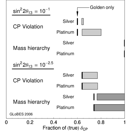
Figure 18: Fraction of true values of $\delta_{CP}$ for which CP violation and a normal mass hierarchy can be established at the $3\sigma$ confidence level for two different values of $\sin^{2}2\theta_{13}$. The baselines are assumed to be 4000 km for all channels and $\mathrm{E_{\mu}=50\,GeV}$. The black lines refer to the performance of the golden detector only, and the gray bars the potential of the additional channel data. The left edges of the bars are for the standard scenarios Silver and Platinum, whereas the right edges of the bars refer to the optimization potentials Silver^∗ and Platinum^∗.

In Figure 18, the contribution from additional silver channel and platinum channel data is discussed for two true values of $\sin^{2}2\theta_{13}$, which represent two conceptually different cases. For a medium $\sin^{2}2\theta_{13}=10^{-2.5}$, the golden channel suffers from degeneracies, and the additional data could help resolve it. For a large $\sin^{2}2\theta_{13}=10^{-1}$, the golden channel suffers from the uncertainty in the matter density and also there, additional channel data could improve the performance. For $\sin^{2}2\theta_{13}\ll 10^{-2.5}$, however, we do not expect major contributions from any of the two channels because of a lack of statistics (silver) or the CID background (platinum). The black lines in Figure 18 refer to the golden channel only, and the improvement from the additional channels is visualized with the bars. The left edges of these bars represent the contribution from the standard scenarios Silver and Platinum, whereas the right edges represent the maximal contribution from the optimistic scenarios Silver^∗ and Platinum^∗. Thus, the finally achievable contribution most likely is within the bars. It can be read off from Figure 18 that the standard scenarios do not contribute in a sizable way, whereas there is a substantial contribution for the optimistic setups. We will therefore only discuss the scenarios Silver^∗ and Platinum^∗ in the following. In the case of a medium $\sin^{2}2\theta_{13}=10^{-2.5}$, the impact of the silver channel and platinum channel is comparable. The sensitivity to the mass hierarchy is restored in the complete $\delta_{CP}$ range, and the fraction of true $\delta_{CP}$ where sensitivity to CP violation is given is significantly increased. However, in the case of the large value of $\sin^{2}2\theta_{13}=10^{-1}$, the platinum channel performs noticeably better than the silver channel. One reason for this, lies in the tau production threshold for the silver channel which suppresses the most useful events around the first oscillation maximum. Note, that already the golden channel alone can distinguish the mass hierarchy over the whole $\delta_{CP}$ range and no improvement can come from the additional channel data.

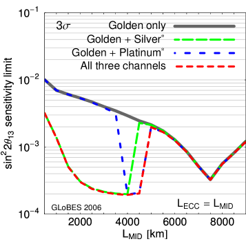
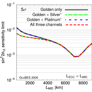
Figure 19: The $\sin^{2}2\theta_{13}$ sensitivity limit for the combination of different channels at $3\sigma$ (left) and $5\sigma$ (right). The energy of the parent muons is fixed to 50 GeV, and systematics, correlations, and degeneracies are taken into account.

As it was shown in Figure 2, the $\sin^{2}2\theta_{13}$ sensitivity suffers from the intrinsic degeneracy, i.e., a second fit solution at $\sin^{2}2\theta_{13}\approx 2.5\times 10^{-3}$ which appears at the $3\sigma$ confidence level. In Figure 19, the sensitivity to $\sin^{2}2\theta_{13}$ is therefore shown at the $3\sigma$ (left) and $5\sigma$ (right) confidence level for the golden channel alone, the combination of golden and silver channel, the combination of golden and platinum channel, and the combination of all three channels as indicated by the plot legend. The baseline of all detectors at the same location is varied between 500 and 9000 km. Again, the effect of the magic baseline at $L\simeq 7500\,\mathrm{km}$ can be easily seen. At $5\sigma$, the degeneracy is still present in all combinations of channels, and the overall sensitivity to $\sin^{2}2\theta_{13}$ is not affected. Only the silver channel improves the achievable limit to some extend at lower baselines. If, however, the $3\sigma$ sensitivity is considered, the silver channel allows to resolve the degeneracy up to baselines of $L\simeq 4000\,\mathrm{km}$, and the platinum channel resolves the degeneracy at $L\simeq 4000\,\mathrm{km}$. In both cases, the sensitivity makes a jump of one order of magnitude in $\sin^{2}2\theta_{13}$, which comes from lifting the degenerate solution in Figure 2 above the $3\sigma$ threshold. However, if one considers the depth of the local $\Delta\chi^{2}$ minimum at $\sin^{2}2\theta_{13}\approx 2.5\times 10^{-3}$, it is only marginally above the $3\sigma$ confidence level. This effect could also be achieved by moderately increasing the detector mass of the golden detector.

Since the silver and platinum channel appearance probabilities have a different dependence in $\delta_{\mathrm{CP}}$, the addition of the data from the two channels should help resolve degeneracies. In order to check the baseline optimization, we show in Figure 20 the sensitivity to the normal mass hierarchy (left) and maximal CP violation (right) for several combinations of channels and $\delta_{\mathrm{CP}}=3\pi/2$, where the degeneracy problem is present.

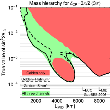
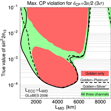
Figure 20: The sensitivity to mass hierarchy (left) and sensitivity to maximal CP violation (right) at $3\sigma$ for the combination of different channels as given in the plot legends. The true value for the CP phase is assumed to be $\delta_{\mathrm{CP}}=3\pi/2$, since for this value the golden channel suffers from the intrinsic degeneracy. All correlations and degeneracies are taken into account.

For the sensitivity to the mass hierarchy (left plot), the additional silver and platinum channel data can improve the sensitivity and close the sensitivity gap between the dark shaded regions in a large baseline window. This implies that the $4\,000\,\mathrm{km}$ baseline alone is very good for the chosen $\delta_{\mathrm{CP}}\approx 3\pi/2$ compared to the magic baseline. We will test in Section 6 if this result holds for all values of $\delta_{\mathrm{CP}}$. We have also checked that the impact of the additional channels is small for $\delta_{\mathrm{CP}}=0$ and even negligible for $\delta_{\mathrm{CP}}=\pi/2$. At this point we would like to point out that the inclusion of the additional silver and platinum channel data does not affect the baseline choice of $4\,000\,\mathrm{km}$. For the maximal CP violation sensitivity (right plot), the best reach of sensitivity to maximal CP violation in small $\sin^{2}2\theta_{13}$ is still obtained at $\mathrm{L\approx 4000\,km}$, while the degeneracy gap can be closed by either of the additional channels. We have not shown the case of the true value $\delta_{\mathrm{CP}}=\pi/2$, but since there the effect of degeneracies is small, we have checked that the impact of the additional channels is negligible in that case for baselines around $4\,000\,\mathrm{km}$.

Besides the baseline optimization, we discuss the muon energy dependence in Appendix A. As the main result, the tau production threshold for the silver channel seems to point to muon energies higher than about $30\,\mathrm{GeV}$.

In this section, we have defined and tested several options for silver and platinum channels, and we have demonstrated their degeneracy resolving potential at individual points in the parameter space. We have shown that the golden channel baseline choice is not affected by the inclusion of the silver channel. In addition, we have found that the platinum channel could be especially useful for large $\sin^{2}2\theta_{13}$, where the impact of the upper CID threshold is lowest. In the next Section 6, we will quantify the synergy of the different channels and other options in terms of the full relevant parameter space. However, we will focus on the optimized setups found in this section (i.e., the “star” options).

6 Comparison of optimized setups

Effort: Baselines $\rightarrow$	One baseline	Two baselines
Detectors $\downarrow$   Overall $\searrow$	(thin curves)	(thick curves)
Single detector	Golden	not applicable
	(Golden)MB
	Beta beam
Double detector	(Golden)2L	Golden+(Golden)MB
	Golden∗
	Golden+Silver∗
	Golden+Platinum∗
Triple detector		Golden∗+(Golden∗)MB
		Golden+(Golden)MB+Platinum∗
Quadruple detector		Golden∗+(Golden∗)MB+Platinum∗

Table 6: Different (optimized) setups considered for comparison. The column headings also contain the line styles used for Figure 21 (for the convenience of comparing similar options). The detector effort is characterized in terms of multiples of a conventional detector: Using an optimized detector, a hybrid detector, additional (optimized) channel, or conventional detector with double luminosity increases the detector effort by one (simplified picture). Therefore, the different rows represent different levels of sophistication in terms of detector, whereas the different columns represent different levels of sophistication in terms of number of baselines. For the muon energy, we use, unless noted otherwise, $E_{\mu}=50\,\mathrm{GeV}$. For all neutrino factory channels, we use, unless noted otherwise, $L=4\,000\,\mathrm{km}$ and $m_{\mathrm{Det}}=50\,\mathrm{kt}$ (a number index refers to a different baseline, “MB” to the magic baseline, and the index $2\mathcal{L}$ refers to double luminosity, i.e., $m_{\mathrm{Det}}=100\,\mathrm{kt}$). The stars refer to the optimized detectors: For the golden channel, a better threshold and energy resolution is implemented, as well as $E_{\mu}=20\,\mathrm{GeV}$ is used for all options including the optimized golden detector; for the silver channel, a $10\,\mathrm{kt}$ ECC with a signal efficiency increased by a factor of five and a background increased by a factor of three is used, which could be achieved by the implementation of more decay channels of the tau lepton; for the platinum channel, the full golden detector mass of $50\,\mathrm{kt}$ is used with an efficiency of 40% in the whole analysis range. For the beta beam, we use the $\gamma=350$ option from Ref. [77] for reference.

In order to compare different neutrino factory options and to discuss where to focus the effort, we use a number of different setups and classify them according to the sophistication of the detection system, the total luminosity, and the number of baselines used. In Table 6, we list these setups in a matrix, where the rows correspond to a similar effort to the detection system, and the columns to an equal number of baselines. We define the “detector effort” in terms of multiples of a conventional detector: Using an optimized detector, a hybrid detector, additional (optimized) channel, or conventional detector with double luminosity/mass increases the detector effort by one. This picture may be a bit over-simplified, since some approaches may be feasible from the current point of view (such as the double mass detector), while others may even not be possible to their full extent (such as the completely optimized detector, or the silver or platinum channels). However, this classification should somehow reflect the level of sophistication in terms of the detection system. For the number of baselines, we restrict ourselves to one or two, i.e., additional detectors/channels have to be placed such that this baseline constraint is not violated. In summary, the effort in Table 6 increases from the top to the bottom in terms of the detection system, from left to right in terms of number of baselines, and diagonally from top left to bottom right in total. Note, however, that an increased detector effort and baseline effort may not be comparable at all, since a second baseline depends on accelerator considerations (such as the storage ring shape), while the increased detector effort is often limited by technical feasibility. Therefore, we visualize these completely different degrees of freedom by the matrix choice in Table 6: The columns represent the accelerator degree of freedom, the rows the detector degree of freedom.

Here we compare optimal setups, i.e., the optimized choices from the previous sections. We do not discuss the baseline and muon energy optimization anymore, but we take the choices for these parameters from the earlier discussion. Let us now quickly explain the setups and their labels as used in Table 6. For the muon energy, we use, unless noted otherwise, $E_{\mu}=50\,\mathrm{GeV}$. For all golden channels, we use $L=4\,000\,\mathrm{km}$ and $m_{\mathrm{Det}}=50\,\mathrm{kt}$, where a number index in the setup refers to a different baseline, and the index “MB” refers to the magic baseline. In addition, the index “$2\mathcal{L}$” refers to double luminosity, i.e., $m_{\mathrm{Det}}=100\,\mathrm{kt}$. The stars refer to the optimized, improved detectors. For the golden channel detector, a better threshold and energy resolution is used, as well as $E_{\mu}=20\,\mathrm{GeV}$ for all options including the optimized golden detector. Therefore, although the setups Golden^∗ represent a detector with a high level of sophistication, the lower muon energy may compensate for this effort. For the silver channel, a $10\,\mathrm{kt}$ ECC with a signal efficiency increased by a factor of five and a background increased by a factor of three is used, which could be achieved by the implementation of more decay channels of the tau lepton. For the platinum channel, the full golden detector mass of $50\,\mathrm{kt}$ is used with an efficiency of 40% in the whole analysis range. Therefore, we use for both silver and platinum channels only the improved setups from the previous section, Silver^∗ and Platinum^∗. Note that wherever the platinum channel is used, it is used in (or at the location of) all golden detectors (such as for Golden+(Golden)_MB+Platinum^∗). In addition, note that the matter density error is assumed to be correlated among all channels at the same baseline. In order to compare the neutrino factory with its possible alternative, a beta beam, we choose the the $\gamma=350$ option from Ref. [77] for reference.

The organization of the section is as follows: First, we will discuss real synergies with respect to the physics potential only, i.e., we compare options which use similar luminosities in terms of flux $\times$ running time $\times$ total detector mass. In the next part, we will discuss specific physics scenarios and how the choice of technology changes with respect to these. And finally, we will focus on the optimized physics potential, where we will demonstrate where to focus the effort.

6.1 Synergies in physics potential

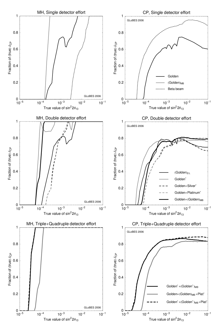
Figure 21: Comparison of the different options from Table 6, where we show the fraction of true $\delta_{\mathrm{CP}}$ as function of true $\sin^{2}2\theta_{13}$ for the normal mass hierarchy sensitivity (left column, $3\sigma$) and CP violation sensitivity (right column, $3\sigma$). The different rows correspond to an increasing detector effort (from top to bottom) corresponding to the rows in Table 6. Note that thin curves represent one-baseline options, and thick curves two-baseline options.

As in Ref. [78], we define the extra gain in the combination of the experiments beyond a simple addition of statistics as the synergy among two or more experiments. A reasonable definition of synergy must therefore subtract, in a suitable way, the increase of statistics of otherwise more or less equivalent experiments. Therefore, from the physics point of view, we restrict the synergy discussion to within the rows in Table 6, since any increase in the detector effort also increases statistics. In order to compare our standard detector to more sophisticated detector combinations (double detector effort), we have incorporated the setup “(Golden)_2L” (second row) with the doubled detector mass. In Figure 21, a comparison of the different options from Table 6 is performed, where we show the fraction of true $\delta_{\mathrm{CP}}$ as function of true $\sin^{2}2\theta_{13}$ for the normal mass hierarchy sensitivity (left column) and CP violation sensitivity (right column). The different rows correspond to an increasing detector effort (from top to bottom) corresponding to the rows in Table 6. Note that thin curves represent one-baseline options, and thick curves two-baseline options. As far as our synergy discussion is concerned, it is taking place within the rows of Figure 21.

The first row in Figure 21 (single detector effort) does not contain any major surprises. For the mass hierarchy, the neutrino factory at the “magic baseline” [55] has the best potential because of the long baseline and reduced degeneracies, which, however, does not have any CP violation sensitivity at all. The neutrino factory faces severe problems with degenerate solutions for intermediate values of $\sin^{2}2\theta_{13}$ (making up the wiggles). The beta beam is extremely good for CP violation measurements, but the relatively short baseline makes the mass hierarchy determination difficult. This property is common to higher gamma beta beams almost independent of the gamma and baseline chosen, because its spectrum easily covers at least one oscillation maximum, but the neutrino energies are too low to go to long baselines with large matter effects (see, e.g., Ref. [15]).

There is a large number of observations from the second row in Figure 21 (double detector effort). One can easily identify synergies by the comparison of the simple luminosity upgrade (golden channel with double luminosity) with the other shown options: Wherever the alternative option is better than the luminosity upgrade, we speak about “synergy” according to our definition, since we gain complementary information to a detector upgrade. For the mass hierarchy, we find such synergies for the silver and platinum channels for intermediate $\sin^{2}2\theta_{13}$, and for the improved detector (Golden^∗) and magic baseline (Golden+(Golden)_MB) even for smaller $\sin^{2}2\theta_{13}$. Note that these latter two options are qualitatively different: For the improved detector, correlations and degeneracies are resolved by increased statistics. Therefore, some “wiggles” at intermediate values of $\sin^{2}2\theta_{13}$ remain. For the magic baseline, statistics is lower because of the $1/L^{2}$ drop of the flux, but correlations and degeneracies are intrinsically not present. For CP violation, we identify the platinum channel and magic baseline to be synergistic for large $\sin^{2}2\theta_{13}$, and the improved detector for small and large $\sin^{2}2\theta_{13}$. Note that the ability of the magic baseline to help for large $\sin^{2}2\theta_{13}$ is new, which comes from the clean measurement of $\sin^{2}2\theta_{13}$ and matter effects without correlation with $\delta_{\mathrm{CP}}$. As far as the silver channel is concerned, we only find very small regions in parameter space where it could be useful compared to the increased golden channel statistics for CP violation, and we have identified much stronger alternatives for the mass hierarchy determination. This means that we do not consider the silver channel for further upgrades anymore. This also because it requires larger muon energies above $E_{\mu}=30\,\mathrm{GeV}$. However, since the platinum channel has the best potential for large $\sin^{2}2\theta_{13}$, we will include it in further discussions.

The last row in Figure 21 represents the most sophisticated neutrino factory setups we could come up with, and all include a second baseline. The option “Golden + (Golden)_MB + Platinum^∗” represents the best option for two baselines if the golden channel detector cannot be improved (and the silver channel is not used). In addition, we include two options “Golden^∗ + (Golden^∗)_MB” and “Golden^∗ + (Golden^∗)_MB + Platinum^∗” with improved detector. One can clearly read off this row that an improved golden detector helps almost everywhere. The platinum channel is, in addition, useful for large $\sin^{2}2\theta_{13}$ (for small $\sin^{2}2\theta_{13}$, the charge identification error limits the potential), whereas it does not improve the mass hierarchy reach for these sophisticated options at all. As the last observation, if one has the choice between R&D for the platinum channel and the improved golden channel detector, one can read off that even for large $\sin^{2}2\theta_{13}$ the improved golden channel is more powerful in combination with the second baseline. In summary, the best neutrino factory setup with two baselines, two improved golden channel detectors, and electron neutrino detection at both detectors could, for the chosen parameter values, measure the mass hierarchy down to $\sin^{2}2\theta_{13}\sim 10^{-4.5}$ and CP violation for most values of $\delta_{\mathrm{CP}}$ down to $\sin^{2}2\theta_{13}\sim 10^{-4}$ at the $3\sigma$ confidence level.

6.2 Performance comparison for specific physics scenarios

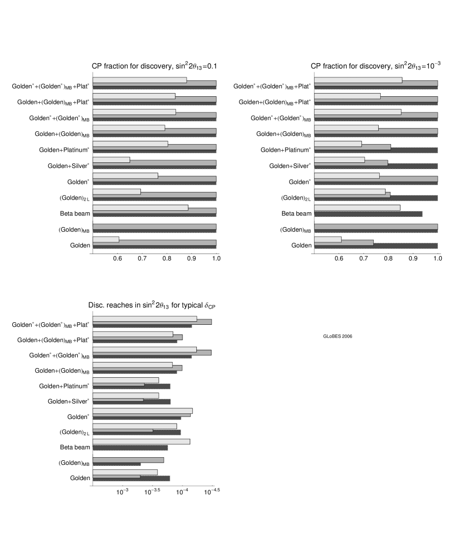
Figure 22: Direct comparison of the $\sin^{2}2\theta_{13}$ (dark bars, $5\sigma$), mass hierarchy (medium bars, $3\sigma$), and CP violation (light bars, $3\sigma$) discovery reaches for the setups from Table 6. The upper left plot shows the fraction of $\delta_{\mathrm{CP}}$ for the physics scenario “large $\sin^{2}2\theta_{13}$” ($\sin^{2}2\theta_{13}=0.1$), the upper right plot the fraction of $\delta_{\mathrm{CP}}$ for the physics scenario “medium $\sin^{2}2\theta_{13}$” ($\sin^{2}2\theta_{13}=10^{-3}$), and the lower plot the $\sin^{2}2\theta_{13}$ discovery reach for the physics scenario “small $\sin^{2}2\theta_{13}$” (for a CP fraction of $0.5$ corresponding to the “typical value of $\delta_{\mathrm{CP}}$”). The detector effort (as defined in Table 6) increases from bottom to top.

As far as the physics scenarios for a neutrino factory are concerned, the main discriminator will certainly be $\sin^{2}2\theta_{13}$. For example, one may distinguish the following scenarios:

Large $\boldsymbol{\sin^{2}2\theta_{13}}$

($\sin^{2}2\theta_{13}\gtrsim 10^{-2}$) In this case, the main question for a neutrino factory is the competitiveness to other options, such as superbeams or beta beams.

Medium $\boldsymbol{\sin^{2}2\theta_{13}}$

($10^{-4}\lesssim\sin^{2}2\theta_{13}\lesssim 10^{-2}$) This is the typical scenario for a neutrino factory. The main focus is on resolving degeneracies.

Small $\boldsymbol{\sin^{2}2\theta_{13}}$

($\sin^{2}2\theta_{13}\lesssim 10^{-4}$) For this range, statistics in combination with low backgrounds is important, which means that the selection of channels and baselines may look differently.

In order to discuss these physics scenarios further, we show in Figure 22 a direct comparison of the $\sin^{2}2\theta_{13}$ (dark bars), mass hierarchy (medium bars), and CP violation (light bars) discovery reaches for the setups from Table 6. The upper left plot shows the fraction of $\delta_{\mathrm{CP}}$ for an example of the physics scenario “large $\sin^{2}2\theta_{13}$” ($\sin^{2}2\theta_{13}=0.1$), the upper right plot the fraction of $\delta_{\mathrm{CP}}$ for one representative example of the physics scenario “medium $\sin^{2}2\theta_{13}$” ($\sin^{2}2\theta_{13}=10^{-3}$), and the lower plot the $\sin^{2}2\theta_{13}$ discovery reach for the physics scenario “small $\sin^{2}2\theta_{13}$” (for a CP fraction of $0.5$ corresponding to the “typical value of $\delta_{\mathrm{CP}}$”). This means that we use the $\sin^{2}2\theta_{13}$ reach as performance indicator for small $\sin^{2}2\theta_{13}$ because it is more discriminating than the CP fraction for a specific value of $\sin^{2}2\theta_{13}$

Let us first discuss the typical interesting range for a neutrino factory (upper right plot). In this example, the $\sin^{2}2\theta_{13}$ discovery is not an issue for any of the neutrino factory options and any value of $\delta_{\mathrm{CP}}$. The mass hierarchy can be measured for all values of $\delta_{\mathrm{CP}}$ by either improving the detector, or by adding the magic baseline. For the measurement of CP violation, however, both of these options may be necessary to increase to physics reach to the optimum and make it competitive to the beta beam. Note that for CP violation alone, increasing the mass of the golden channel detector may be better than adding the second baseline because of the better statistics. As far as the overall comparison with the beta beam is concerned, a superior performance for the neutrino factory can be easily established with respect to $\sin^{2}2\theta_{13}$ and mass hierarchy discovery, whereas the improved detector and second baseline will allow for the best physics potential for all shown performance indicators.

For small values of $\sin^{2}2\theta_{13}$, the $\sin^{2}2\theta_{13}$ discovery reach is shown in the lower panel of Figure 22. In this case, the optimal reach for all indicators can clearly be obtained by an improved detector operated at two baselines “Golden^∗+(Golden^∗)_MB”, where the magic baseline is a key component to improve the mass hierarchy reach. The final potential for each of the three performance indicators is significantly better than the one of the beta beam. However, note that also the golden channel alone performs already fairly well, since correlations and degeneracies are less important than statistics in this regime.

For large values of $\sin^{2}2\theta_{13}$ (upper left plot in Figure 22), we find that neither the mass hierarchy nor the $\sin^{2}2\theta_{13}$ discovery are a problem for any $\delta_{\mathrm{CP}}$ or option. Thus, the performance comparison reduces to the CP violation potential. One can read off this figure that the potential of the neutrino factory can be significantly improved by adding the magic baseline, utilizing the platinum channel, or improving the golden channel detector. In principle, one can also think about a re-optimization of the final configuration in two-baseline space using all available channels and improvements. Although we find that this could increase the CP violation potential slightly (such as using a $L=1\,500\,\mathrm{km}$ baseline instead of the very long baseline), it is hard to compete with the beta beam in the entire range $\sin^{2}2\theta_{13}\gtrsim 0.01$. Therefore, even after all of these improvements, there is no clear advantage compared to the beta beam, which serves as a representative for a number of circulating beta beam and superbeam upgrade options at this place.

In summary, we have demonstrated that one might optimize a neutrino factory for extremely good performances in $\sin^{2}2\theta_{13}$, mass hierarchy, and CP violation discovery reach below $\sin^{2}2\theta_{13}\lesssim 10^{-2}$. This means that we believe it to be difficult for alternative options to compete in this range for all of these specific performance indicators. However, we cannot establish the physics case for a neutrino factory for $\sin^{2}2\theta_{13}\gtrsim 0.01$ for sure. This means that depending on systematics and achievable luminosities for alternative options (beta beams, superbeams), as well as the utilization of the platinum channel and the improvement of the golden detector at the neutrino factory, alternative options could actually be better for CP violation. Note that for large $\sin^{2}2\theta_{13}$, the $\sin^{2}2\theta_{13}$ and mass hierarchy discoveries are very likely possible with many alternatives.

6.3 Where to concentrate the efforts?

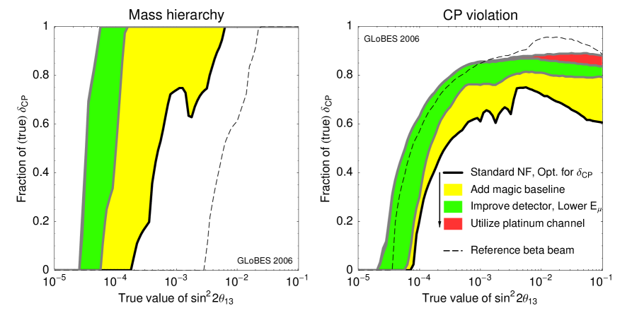
Figure 23: Summary of the optimization potential of a neutrino factory for mass hierarchy (left) and CP violation (right) at the $3\sigma$ confidence level. The different shaded areas correspond to successively taking into account the additional optimizations as given in the plot legend. This means, for instance, that the best curves include both magic baseline and (improved) platinum channels. For reference, we show the $\gamma=350$ beta beam from Ref. [77].

Given the discussions in the last two subsections, let us summarize the results of the optimization and where to concentrate the efforts.

For the optimal baseline, we find that CP violation measurements favor a baseline around $4\,000\,\mathrm{km}$, where baselines between $3\,000\mathrm{km}$ and $5\,000\,\mathrm{km}$ do not affect the sensitivity too much. For large values of $\sin^{2}2\theta_{13}$, shorter baselines $L\gtrsim 1\,500\,\mathrm{km}$ are possible as well. Note that the “short” baseline ($L\lesssim 5\,000\,\mathrm{km}$) is affected by correlations and degeneracies for small and intermediate values of $\sin^{2}2\theta_{13}$, which means that it has moderate $\sin^{2}2\theta_{13}$ and mass hierarchy sensitivities. In addition, we have tested this optimization result for larger values of $\Delta m_{31}^{2}$, and it does not change significantly (whereas the absolute physics potential increases).

As far as baseline upgrades are concerned, a degeneracy resolving baseline is necessary to improve the $\sin^{2}2\theta_{13}$ sensitivity, $\sin^{2}2\theta_{13}$ discovery reach, and mass hierarchy discovery reach. The “magic baseline” at $L\sim 7\,000\,\mathrm{km}-7\,500\,\mathrm{km}$ is a very robust such degeneracy resolver (independent of the oscillation parameters, possibly over-estimated luminosities, chosen confidence level, etc.) because the appearance probability does not depend on $\delta_{\mathrm{CP}}$ there and the ($\delta_{\mathrm{CP}},\theta_{13}$)-degeneracy can be unambiguously resolved. Furthermore, matter effects are stronger than for the shorter baseline, which means that the magic baseline measures a different physics instead of being a pure luminosity upgrade. In addition, it helps for CP violation measurements at large $\sin^{2}2\theta_{13}$, and can establish the MSW effect in Earth matter even for $\sin^{2}2\theta_{13}=0$ [24]. Since this baseline is useful in all physics scenarios, one may want to choose a storage ring and neutrino factory setup with two baselines already from the very beginning.

For detector upgrades, an improvement of the golden channel detector is certainly the main objective. Especially, improving the detection threshold will greatly improve the physics potential in all physics scenarios and for both mass hierarchy and CP violation measurements. In particular, we have demonstrated that an improved detector would allow to use a lower $E_{\mu}\sim 20\,\mathrm{GeV}$ instead of $E_{\mu}\sim 50\,\mathrm{GeV}$, which means that the effort on the accelerator side would be much lower. However, note that an improved detector will not be able to solve all degeneracy issues on its own.

In addition, as an independent effort for useful additional channels, the platinum channel (electron neutrino detection) will be very useful for large $\sin^{2}2\theta_{13}\gtrsim 10^{-2}$ if the assumed level of charge identification can be achieved up to large enough energies (about $10$ to $15\,\mathrm{GeV}$, cf., Figure 17), and enough statistics can be collected. This improvement would also be complementary to the improved detector from the theoretical point of view, since a different combination of CP violation and matter effects would be measured (the channel behaves like an antineutrino channel with neutrino matter effects, i.e., it is the T-conjugated channel to the golden channel). However, it should be secondary objective after improving the golden channel detection threshold. In addition, the silver channel might be useful for a small fraction of the parameter space for relatively large detectors and enough tau decay channels implemented to improve statistics. Note that the silver channel could be interesting for different applications not tested here, such as new physics tests or deviations from maximal mixing.

The muon energy for a neutrino factory should be around $40$ to $50\,\mathrm{GeV}$ in order to be optimized for all measurements, where it may not have to be as high as $50\,\mathrm{GeV}$ for neutrino oscillation physics because of the matter resonance in the Earth’s mantle. An improvement of the detection threshold could reduce the muon energy to $20\,\mathrm{GeV}$ while having excellent physics sensitivities, and the physics scenario “large $\sin^{2}2\theta_{13}$” may even allow for lower energies (while $50\,\mathrm{GeV}$ do not harm). Note that the use of the silver channel disfavors too low muon energies, i.e., $E_{\mu}$ should in this case be larger than about $30\,\mathrm{GeV}$.

We show in Figure 23 the summary of this optimization discussion by successively switching on the second baseline, by improving the detector performance, and by using the platinum channel (Platinum^∗). We have chosen this order because it we believe that it somehow represents the order of the technical feasibility at this point of time. The second baseline will be a major challenge from the engineering point of view. However, the physics potential of this baseline is well established and the technical feasibility should be rather predictable. The improvement of the detector with respect to energy resolution and threshold should be doable to a certain extent, but it is not yet clear yet by how much exactly. The platinum channel may be implemented in the golden detector, but the electron neutrino detection may turn out to be technically not doable at this level and might be limited to too low energies. In this figure, the beta beam curves are once again given for reference. One can easily read off the excellent combined potential for mass hierarchy and CP violation for the neutrino factory below $\sin^{2}2\theta_{13}\lesssim 10^{-2}$. Remember that none of these suggested improvements could be achieved with a simple luminosity upgrade, i.e., adding mass to the golden channel detector. Therefore, we speak of real synergies.

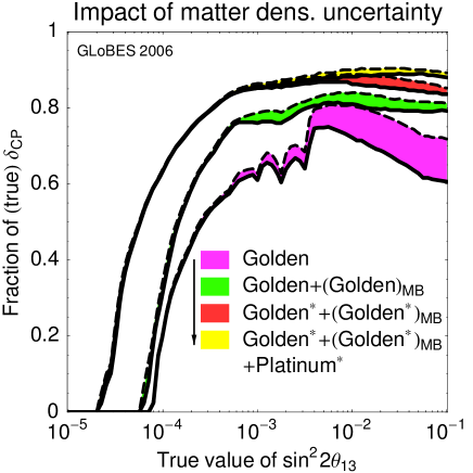
Figure 24: Curves from Figure 23 (right) for 5% matter density uncertainty (solid) and 2% matter density uncertainty (dashed), i.e., the shaded areas represent the improvement potential with respect to the unknown matter density profile. Note, that in going from Golden to Golden* the muon energy goes down from $E_{\mu}=50\,\mathrm{GeV}$ to $E_{\mu}=20\,\mathrm{GeV}$.

Finally, it is well known that the matter density uncertainty is important for $\sin^{2}2\theta_{13}$ and $\delta_{\mathrm{CP}}$ measurements at large $\sin^{2}2\theta_{13}$ (see, e.g., Refs. [20, 64] for the relevant regions in parameter space). Since magic baseline and platinum channel extract the information on $\sin^{2}2\theta_{13}$ (and $\delta_{\mathrm{CP}}$) in a different way compared to the golden channel, one may suspect that the correlation with the matter density can be partially eliminated. We therefore test the impact of the matter density uncertainty on our optimization summary in Figure 24. Obviously, for the $L=4\,000\mathrm{km}$ baseline alone, the impact of matter density uncertainties is rather large (“Golden”). However, especially the magic baseline and platinum channel reduce this dependency. This result is very interesting, since it means that using magic baseline and possibly platinum channel, an improvement of the knowledge on the matter density profile may not be necessary anymore. Nevertheless, note that a lower matter density uncertainty cannot replace the detector, channel, and baseline improvements discussed in this section.

7 Summary and conclusions

In this study, we have optimized a neutrino factory for oscillation parameter measurements. Assuming the standard magnetized iron calorimeter as detector we find the following results: For small $\sin^{2}2\theta_{13}$, we have found an excellent (maximal) CP violation sensitivity for baselines $L\simeq 3\,000\,\mathrm{km}$ to $5\,000\,\mathrm{km}$, mass hierarchy sensitivity for $L\gtrsim 6\,000\,\mathrm{km}$, and $\sin^{2}2\theta_{13}$ sensitivity at the “magic baseline” $L\simeq 7\,500\,\mathrm{km}$. Thus, the optimal baseline depends on the performance indicator one is optimizing for. In summary, we have identified the combination of two baselines $L\sim 4\,000\,\mathrm{km}$ and $L\simeq 7\,500\,\mathrm{km}$ as the optimal configuration given these different performance indicators. For the muon energy, we have found that $E_{\mu}\gtrsim 40\,\mathrm{GeV}$ should be sufficient. Note that a longer baseline (such as the $L\simeq 7\,500\,\mathrm{km}$) is useful for the $\pi/2-\theta_{23}$ measurement as well as for seeing multiple oscillation nodes.

For large $\sin^{2}2\theta_{13}$, the determination of the mass hierarchy and $\sin^{2}2\theta_{13}$ discovery are not a problem at all. Therefore, the optimization is determined by the CP violation sensitivity. We have found that in this case slightly shorter baselines $L\gtrsim 1\,500\,\mathrm{km}$ and lower muon energies $E_{\mu}\gtrsim 20\,\mathrm{GeV}$ are sufficient, while the values identified for small $\sin^{2}2\theta_{13}$ do not harm. In addition, the “magic baseline” improves the CP violation measurement potential because of a “clean” (i.e. unaffected by $\delta_{\mathrm{CP}}$) measurement of $\sin^{2}2\theta_{13}$.

In order to further improve the neutrino factory, we have demonstrated that a lower energy threshold and higher energy resolution for the muon neutrino (golden channel) detector would increase the physics potential significantly. In that case, also, the muon energy can be reduced to $E_{\mu}=20\,\mathrm{GeV}$. In particular, the lower energy threshold increases the mass hierarchy and CP violation discovery reaches. This statement is true even in the presence of a higher background fraction from neutral currents and mis-identified events. For large $\sin^{2}2\theta_{13}$, we have found that all of the following help for a single detector/baseline: lower threshold, better energy resolution, and lower matter density uncertainties. Therefore, improving the golden channel detector will have an excellent potential to push the neutrino factory physics reach independently of the value of $\theta_{13}$. Further studies are needed to demonstrate to what extent the detector improvements, we have anticipated, can be achieved.

As far as different channels are concerned, we have modeled electron (platinum channel) and tau (silver channel) neutrino appearance. Due to the assumption of standard oscillations of three active flavors, the additional channels do not provide completely independent information. From an experimental point of view, both channels represent a considerably more difficult challenge than the golden channel. As a consequence the number of events in either the silver or platinum channel will typically be smaller than the one in the golden channel, and the backgrounds always will be higher, which means that the statistical significance is doubly suppressed. Therefore, additional channels can only improve the physics reach of the golden channel in those regions of parameter space where the performance of the golden channel alone is sub-optimal. The two regions where this happens are either large $\sin^{2}2\theta_{13}\sim 0.1$, where the matter density uncertainty spoils the sensitivity to CP violation, or intermediate $\sin^{2}2\theta_{13}\sim 3\times 10^{-3}$, where the so-called $\pi$-transit of the mass hierarchy degeneracy can destroy CP violation and mass hierarchy sensitivities. For the standard configurations of both channels using currently accepted parameter estimates, we found that the impact is small in comparison to the additional effort. Therefore, we have considered improved versions of these channels throughout this study, which we have introduced as Silver^∗ and Platinum^∗. The improvements with respect to the standard setups are mainly much larger statistics (factor 5-10) and lower backgrounds (Silver^∗), as well as a wider energy range for charge identification (Platinum^∗). These improvements are, at current, hypothetical, and more detector studies are clearly needed. We have demonstrated that the improved platinum channel is especially helpful for large $\sin^{2}2\theta_{13}$, where the impact of the upper CID threshold is moderate. For intermediate values of $\sin^{2}2\theta_{13}$, we find that both the improved silver and platinum channel can resolve the effects of the $\pi$-transit. However, the platinum channel requires a much higher CID threshold in this range. Note that we have not tested the use of the silver channel for significant deviations from maximal mixing and for new physics test, which are under discussion elsewhere (see, e.g., Refs. [73, 37]). In summary, the addition of silver and platinum channels is most likely only justified by their ability to provide crucial cross checks of the assumption of standard three flavor oscillation.

In the last part of this study, we have compared different options for synergies and competitiveness including the option of multiple baselines, as well as we have compared the neutrino factory to a higher gamma beta beam representative. We have found that magic baseline, improved golden detector, and platinum channels are synergistic at a varying degree and competitive in different regions of the parameter space. Thus, the same physics potential cannot just be achieved by increasing the luminosity. In addition, we have shown that a neutrino factory can outperform the competing technologies, such as beta beams, for $\sin^{2}2\theta_{13}\lesssim 10^{-2}$. This is especially true with respect to the fact that a neutrino factory can address all open issues in oscillation physics. For large $\sin^{2}2\theta_{13}\gtrsim 10^{-2}$, we have demonstrated that improving the golden channel detector, adding the magic baseline, and using the platinum channel would improve the physics potential. We have also found that the use of magic baseline and platinum channel reduces the impact of matter density uncertainties for large $\sin^{2}2\theta_{13}$ significantly, i.e., the more information is added, the less important the matter density uncertainties become. However, it is yet unclear if not other alternatives, such as higher gamma beta beams, can do the desired measurements with a lower effort, which very much depends on the systematics assumed for these experiments.

We conclude that the neutrino factory setup optimized for oscillation parameter measurements has two baselines, one at $L\sim 4000\,\mathrm{km}$ and one at $L\simeq 7\,500\,\mathrm{km}$, an optimized golden channel detector with lower threshold and higher energy resolution and a muon energy of $E_{\mu}\sim 20\,\mathrm{GeV}$. This set of improvements exhausts the optimization potential in the majority of the parameter space. The only region where an additional gain may be achieved is for large $\sin^{2}2\theta_{13}\sim 0.1$. Here the addition of a high statistics platinum channel detector would decrease the impact of the matter density uncertainty.

As far as future neutrino factory R&D is concerned, we find that the ability to operate two baselines as well as the lower detection threshold of the golden detector are the most critical components to the optimized physics potential. Furthermore, a better energy resolution of the golden channel detector would improve the physics potential further.

Appendix A Impact of muon energy on additional channels

Besides the baseline, the muon energy (energy of the muons stored in the storage ring) can be changed. In the former discussions of additional channel data this parameter was set to the standard neutrino factory value $E_{\mu}=50\,\mathrm{GeV}$. A reduction of the muon energy may be especially interesting in connection with an improved detector, as well as it may allow to use a larger fraction of the platinum channel data if the upper platinum CID threshold is at lower energies. On the other hand, the tau production threshold may affect the usefulness of the silver channel for lower muon energies. Therefore, we discuss in this appendix if the inclusion of additional channel information changes the muon energy optimization.

As far as the sensitivity to the normal mass hierarchy is concerned, we show in Figure 25 (left) the relevant $\sin^{2}2\theta_{13}$ reach $L_{\mathrm{MID}}=L_{\mathrm{ECC}}=4000\,\mathrm{km}$. The variation of the absolute reach in small values of true $\sin^{2}2\theta_{13}$ is of minor importance, and even improves slightly for the choice of smaller parent energies. For the golden channel only, or golden and platinum channels combined, the optimum is approximately reached for $E_{\mu}\sim 30\,\mathrm{GeV}$. The lack of sensitivity to the mass hierarchy in the gap between the dark gray-shaded regions cannot be resolved by the golden channel alone independent of $\mathrm{E_{\mu}}$. However, if combined with the silver or platinum channel, the sensitivity gap can be closed for parent energies $E_{\mu}\gtrsim 20\,\mathrm{GeV}$ (platinum combinations) or larger than about $E_{\mu}\gtrsim 25\,\mathrm{GeV}$ (golden and silver combined). For the platinum combinations (or all channels combined), the additional channel information does not only allow to use a lower energy neutrino beam, but also favors a lower parent energy of $E_{\mu}\sim 30\,\mathrm{GeV}$. If, on the other hand, only the silver channel data is used, the tau production threshold disfavors too low muon energies.

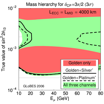
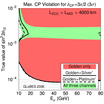
Figure 25: The sensitivity to the normal mass hierarchy (left) and to maximal CP violation (right) at $3\sigma$ for the combination of different channels as given in the plot legend. The true value of the phase is assumed to be $\delta_{\mathrm{CP}}=3\pi/2$, and the hierarchy is assumed to be normal. The parent energy of the stored muons is varied and the baseline is fixed to $L_{\mathrm{MID}}=L_{\mathrm{ECC}}=4000\,\mathrm{km}$

On the right-hand side of Figure 25, the sensitivity to maximal CP violation is shown as function of the muon energy. The qualitative observations are the same as for the mass hierarchy, but the silver channel favors $\mathrm{E_{\mu}\gtrsim 20\,GeV}$.

References

- [1] G. L. Fogli, E. Lisi, A. Marrone, and A. Palazzo (2005), hep-ph/0506083.
- [2] T. Schwetz (2006), hep-ph/0606060.
- [3] A. Aguilar et al. (LSND), Phys. Rev. D64, 112007 (2001), hep-ex/0104049.
- [4] H. Minakata, H. Sugiyama, O. Yasuda, K. Inoue, and F. Suekane, Phys. Rev. D68, 033017 (2003), hep-ph/0211111.
- [5] P. Huber, M. Lindner, T. Schwetz, and W. Winter, Nucl. Phys. B665, 487 (2003), hep-ph/0303232.
- [6] K. Anderson et al. (2004), hep-ex/0402041.
- [7] F. Ardellier et al. (2004), hep-ex/0405032.
- [8] E. Ables et al. (MINOS) FERMILAB-PROPOSAL-P-875.
- [9] Y. Itow et al. (2001), hep-ex/0106019.
- [10] D. S. Ayres et al. (NOvA) (2004), hep-ex/0503053.
- [11] S. Geer, Phys. Rev. D57, 6989 (1998), hep-ph/9712290.
- [12] C. Albright et al. (2000), hep-ex/0008064.
- [13] M. Apollonio et al. (2002), hep-ph/0210192.
- [14] J. Burguet-Castell, D. Casper, J. J. Gomez-Cadenas, P. Hernandez, and F. Sanchez, Nucl. Phys. B695, 217 (2004), hep-ph/0312068.
- [15] P. Huber, M. Lindner, M. Rolinec, and W. Winter, Phys. Rev. D73, 053002 (2006), hep-ph/0506237.
-
[16]
V. Barger,
S. Geer, and
K. Whisnant,
Phys. Rev. D61,
053004 (2000),
hep-ph/9906487. - [17] A. Cervera et al., Nucl. Phys. B579, 17 (2000), hep-ph/0002108.
- [18] J. Burguet-Castell, M. B. Gavela, J. J. Gomez-Cadenas, P. Hernandez, and O. Mena, Nucl. Phys. B608, 301 (2001), hep-ph/0103258.
- [19] M. Freund, P. Huber, and M. Lindner, Nucl. Phys. B615, 331 (2001), hep-ph/0105071.
- [20] P. Huber, M. Lindner, and W. Winter, Nucl. Phys. B645, 3 (2002), hep-ph/0204352.
- [21] P. Huber, M. Lindner, and W. Winter, JHEP 05, 020 (2005), hep-ph/0412199.
- [22] A. Donini, E. Fernandez-Martinez, D. Meloni, and S. Rigolin, Nucl. Phys. B743, 41 (2006), hep-ph/0512038.
- [23] M. Freund, P. Huber, and M. Lindner, Nucl. Phys. B585, 105 (2000), hep-ph/0004085.
- [24] W. Winter, Phys. Lett. B613, 67 (2005), hep-ph/0411309.
- [25] A. de Gouvea, J. Jenkins, and B. Kayser, Phys. Rev. D71, 113009 (2005), hep-ph/0503079.
- [26] A. de Gouvea and W. Winter, Phys. Rev. D73, 033003 (2006), hep-ph/0509359.
- [27] W. Winter, Phys. Rev. D72, 037302 (2005), hep-ph/0502097.
- [28] T. Ota, J. Sato, and N.-a. Yamashita, Phys. Rev. D65, 093015 (2002), hep-ph/0112329.
- [29] P. Huber, T. Schwetz, and J. W. F. Valle, Phys. Rev. D66, 013006 (2002), hep-ph/0202048.
- [30] P. Huber, T. Schwetz, and J. W. F. Valle, Phys. Rev. Lett. 88, 101804 (2002), hep-ph/0111224.
- [31] M. Campanelli and A. Romanino, Phys. Rev. D66, 113001 (2002), hep-ph/0207350.
- [32] M. Garbutt and B. H. J. McKellar (2003), hep-ph/0308111.
- [33] V. Barger, S. Geer, and K. Whisnant, New J. Phys. 6, 135 (2004), hep-ph/0407140.
- [34] M. Blennow, T. Ohlsson, and W. Winter, JHEP 06, 049 (2005), hep-ph/0502147.
- [35] M. Blennow, T. Ohlsson, and W. Winter (2005), hep-ph/0508175.
- [36] T. Ota and J. Sato, Phys. Rev. D71, 096004 (2005), hep-ph/0502124.
- [37] N. Kitazawa, H. Sugiyama, and O. Yasuda (2006), hep-ph/0606013.
- [38] F. R. Klinkhamer, Phys. Rev. D73, 057301 (2006), hep-ph/0601116.
- [39] S. Davidson, C. Pena-Garay, N. Rius, and A. Santamaria, JHEP 03, 011 (2003), hep-ph/0302093.
- [40] M. L. Mangano et al. (2001), hep-ph/0105155.
- [41] V. D. Barger, K. Whisnant, and R. J. N. Phillips, Phys. Rev. Lett. 45, 2084 (1980).
- [42] A. De Rujula, M. B. Gavela, and P. Hernandez, Nucl. Phys. B547, 21 (1999), hep-ph/9811390.
- [43] K. Dick, M. Freund, M. Lindner, and A. Romanino, Nucl. Phys. B562, 29 (1999), hep-ph/9903308.
- [44] A. Donini, M. B. Gavela, P. Hernandez, and S. Rigolin, Nucl. Phys. B574, 23 (2000), hep-ph/9909254.
- [45] M. Freund, M. Lindner, S. T. Petcov, and A. Romanino, Nucl. Phys. B578, 27 (2000), hep-ph/9912457.
- [46] J. Arafune, M. Koike, and J. Sato, Phys. Rev. D56, 3093 (1997), hep-ph/9703351.
- [47] H. Minakata and H. Nunokawa, Phys. Lett. B413, 369 (1997), hep-ph/9706281.
- [48] H. Minakata and H. Nunokawa, Phys. Rev. D57, 4403 (1998), hep-ph/9705208.
- [49] M. Tanimoto, Phys. Lett. B435, 373 (1998), hep-ph/9806375.
- [50] M. Freund, Phys. Rev. D64, 053003 (2001), hep-ph/0103300.
- [51] E. K. Akhmedov, R. Johansson, M. Lindner, T. Ohlsson, and T. Schwetz, JHEP 04, 078 (2004), hep-ph/0402175.
- [52] V. Barger, D. Marfatia, and K. Whisnant, Phys. Rev. D65, 073023 (2002), hep-ph/0112119.
- [53] H. Minakata and H. Nunokawa, JHEP 10, 001 (2001), hep-ph/0108085.
- [54] G. L. Fogli and E. Lisi, Phys. Rev. D54, 3667 (1996), hep-ph/9604415.
- [55] P. Huber and W. Winter, Phys. Rev. D68, 037301 (2003), hep-ph/0301257.
- [56] A. Donini, D. Meloni, and P. Migliozzi, Nucl. Phys. B646, 321 (2002), hep-ph/0206034.
- [57] A. Bueno, M. Campanelli, S. Navas-Concha, and A. Rubbia, Nucl. Phys. B631, 239 (2002), hep-ph/0112297.
- [58] P. Huber, M. Lindner, and W. Winter, Comput. Phys. Commun. 167, 195 (2005), http://www.ph.tum.de/∼globes, hep-ph/0407333.
- [59] M. Maltoni, T. Schwetz, M. A. Tortola, and J. W. F. Valle, New J. Phys. 6, 122 (2004), hep-ph/0405172.
- [60] G. L. Fogli, E. Lisi, A. Marrone, and D. Montanino, Phys. Rev. D67, 093006 (2003), hep-ph/0303064.
- [61] J. N. Bahcall, M. C. Gonzalez-Garcia, and C. Pena-Garay, JHEP 08, 016 (2004), hep-ph/0406294.
- [62] A. Bandyopadhyay, S. Choubey, S. Goswami, S. T. Petcov, and D. P. Roy (2004), hep-ph/0406328.
- [63] R. J. Geller and T. Hara, Nucl. Instrum. Meth. A503, 187 (2001), hep-ph/0111342.
- [64] T. Ohlsson and W. Winter, Phys. Rev. D68, 073007 (2003), hep-ph/0307178.
- [65] P. Huber, M. Lindner, M. Rolinec, T. Schwetz, and W. Winter, Phys. Rev. D70, 073014 (2004), hep-ph/0403068.
- [66] N. Tagg (the MINOS) (2006), hep-ex/0605058.
- [67] S. Antusch, P. Huber, J. Kersten, T. Schwetz, and W. Winter, Phys. Rev. D70, 097302 (2004), hep-ph/0404268.
- [68] S. V. Panasyuk, Rem (reference earth model) web page (2000), http://cfauvcs5.harvard.edu/lana/rem/index.htm.
- [69] ISS detector working group, private communication.
- [70] A. Cervera, F. Dydak, and J. Gomez Cadenas, Nucl. Instrum. Meth. A451, 123 (2000).
- [71] I. Ambats et al. (NOvA) FERMILAB-PROPOSAL-0929.
- [72] P. Huber, J. Kopp, M. Lindner, M. Rolinec, and W. Winter, JHEP (to be published), hep-ph/0601266.
- [73] D. Autiero et al., Eur. Phys. J. C33, 243 (2004), hep-ph/0305185.
- [74] P. Migliozzi, private communication.
- [75] M. Diwan et al. (MINOS), A study of sensitivity in MINOS, Tech. Rep. NuMI-L-714 (2001).
- [76] A. Rubbia (2001), hep-ph/0106088.
- [77] J. Burguet-Castell, D. Casper, E. Couce, J. J. Gomez-Cadenas, and P. Hernandez, Nucl. Phys. B725, 306 (2005), hep-ph/0503021.
- [78] P. Huber, M. Lindner, and W. Winter, Nucl. Phys. B654, 3 (2003), hep-ph/0211300.