$pp\rightarrow jje^{\pm}\mu^{\pm}\nu\nu$ and $jje^{\pm}\mu^{\mp}\nu\nu$ at ${\cal O}(\alpha_{\rm em}^{6})$ and ${\cal O}(\alpha_{\rm em}^{4}\alpha_{s}^{2})$ for the Study of the Quartic Electroweak Gauge Boson Vertex at LHC

Abstract

We analyze the potential of the CERN Large Hadron Collider (LHC) to study the structure of quartic vector–boson interactions through the pair production of electroweak gauge bosons via weak boson fusion $qq\to qqWW$. In order to study these couplings we have performed a partonic level calculation of all processes $pp\rightarrow jje^{\pm}\mu^{\pm}\nu\nu$ and $pp\rightarrow jje^{\pm}\mu^{\mp}\nu\nu$ at the LHC using the exact matrix elements at ${\cal O}(\alpha_{\rm em}^{6})$ and ${\cal O}(\alpha_{\rm em}^{4}\alpha_{s}^{2})$ as well as a full simulation of the $t\bar{t}$ plus 0 to 2 jets backgrounds. A complete calculation of the scattering amplitudes is necessary not only for a correct description of the process but also to preserve all correlations between the final state particles which can be used to enhance the signal. Our analyses indicate that the LHC can improve by more than one order of magnitude the bounds arising at present from indirect measurements.

I Introduction

Within the framework of the Standard Model (SM), the structure of the trilinear and quartic vector boson couplings is completely determined by the $SU(2)_{L}\times U(1)_{Y}$ gauge symmetry. The study of these interactions can either lead to an additional confirmation of the model or give some hint on the existence of new phenomena at a higher scale anomalous . The triple gauge–boson couplings were probed at the LEP lep ; exp:LEP and are still under scrutiny at the Tevatron teva through the production of vector boson pairs. However, we have only started to study directly the quartic gauge–boson couplings exp:LEP . If any deviation from the SM predictions is observed, independent tests of the triple and quartic gauge–boson couplings can give important information on the type of new physics responsible for the departures from the SM. For example, the exchange of heavy bosons can generate a tree level contribution to four gauge–boson couplings while its effect in the triple–gauge vertex would only appear at one–loop level, and consequently be suppressed with respect to the quartic one aew .

At present the scarce experimental information on quartic anomalous couplings arises from the processes $e^{+}e^{-}\rightarrow W^{+}W^{-}\gamma$, $Z\gamma\gamma$, $ZZ\gamma$, and $\nu\bar{\nu}\gamma\gamma$ at LEP exp:LEP . Due to phase space limitations, the best sensitivity is attainable for couplings involving photons which should appear in the final state. Photonic quartic anomalous couplings can also affect $\gamma\gamma Z$ and $\gamma\gamma W$ productions at Tevatron our:quartic ; stir2 and they will be further tested at LHC our:quartic2 and in the long term at the next generation $e^{+}e^{-}$ collider Belanger:1999aw ; nlc ; bel:bou ; ggnos ; our:vvv .

Purely electroweak quartic couplings $W^{+}W^{-}W^{+}W^{-}$ and $W^{+}W^{-}ZZ$ have not been directly tested so far but will be within reach at LHC bagger0 ; bagger ; dobado ; Belyaev:1998ih . In this work we study the potential of the LHC to probe them by performing a detailed analysis of the most sensitive channels that are the production via weak boson fusion (WBF) of $W^{+}W^{-}$ pairs accompanied by jets, i.e.,

$$p+p\to jjW^{+}W^{-}\to jje^{\pm}\mu^{\mp}\nu\nu\;,$$ (1)

and the WBF production of a pair of jets plus $W^{\pm}W^{\pm}$

$$p+p\to jjW^{\pm}W^{\pm}\to jje^{\pm}\mu^{\pm}\nu\nu\;.$$ (2)

We have only considered final state with different flavor leptons ($e$ and $\mu$) in order to avoid backgrounds coming from $Z,\gamma\to e^{+}e^{-}$ or $\mu^{+}\mu^{-}$. The advantage of WBF, where the scattered final–state quarks receive significant transverse momentum and are observed in the detector as far-forward/backward jets, is the strong reduction of QCD backgrounds due to the kinematic configuration of the colored part of the event.

There are previous studies of the quartic gauge boson couplings at the LHC. The earlier works bagger0 ; bagger ; dobado relied upon the equivalence theorem equ or/and the effective $W$–boson approximation evb . In Ref. Belyaev:1998ih the full tree level calculation of the processes $pp\to VV+$ 2 jets, with $V=W^{\pm},Z^{0}$ was presented. Here, we improve over these earlier works by computing the full matrix element for all processes with the six fermion final states in (1) and (2) at ${\cal O}(\alpha_{\rm em}^{6})$ and ${\cal O}(\alpha_{\rm em}^{4}\alpha_{s}^{2})$. This includes the contribution from the resonant gauge boson pair production considered in Ref. Belyaev:1998ih as well as all the non–resonant contributions and their interference. We have also performed a full simulation of the $t\bar{t}$ background and evaluated the $t\bar{t}$ plus 1 and 2 jets backgrounds using the narrow width approximation for the top.

The interactions responsible for the electroweak symmetry breaking play an important role in the gauge–boson scattering at high energies as they are an essential ingredient to avoid unitarity violation in the scattering amplitudes of massive vector bosons at the TeV scale unit . There are two possible forms of electroweak symmetry breaking which lead to different solutions to the unitarity problem: $(a)$ there is a particle lighter than 1 TeV, the Higgs boson in the standard model, or $(b)$ such particle is absent and the longitudinal components of the $W$ and $Z$ bosons become strongly interacting at high energies. In the latter case, the symmetry breaking occurs due to the nonzero vacuum expectation value of some composite operators which are related with new underlying physics.

We parameterize in a model independent form the possible deviations of the SM predictions for the $W^{+}W^{-}W^{+}W^{-}$ and $W^{+}W^{-}ZZ$ quartic gauge couplings in these two different scenarios as described in Sec. II. In the first case we assume the existence of a light Higgs boson and consequently we are lead to dimension eight effective operators where the $SU(2)_{L}\times U(1)_{Y}$ gauge invariance is realized linearly. We also contemplate the scenario where no new heavy resonance has been observed that leads to the gauge symmetry being realized nonlinearly by using the chiral Lagrangian approach.

Valuable information on the possibility of new physics effects can also be gathered from the low energy data and the results of the $Z$ physics; see Ref. Barbieri:2004qk for a recent review. In particular they can constrain the possible deviations of the quartic gauge boson self–interactions from the SM predictions through their contributions to the electroweak radiative corrections Brunstein:1996fz . For completeness we present in Sec. III the updated bounds on these effects from the global electroweak fit.

Sections IV and V contain the details of the strategies proposed to reduce the backgrounds to acceptable levels while keeping the signal from the quartic gauge vertex. We find that the complete calculation of the scattering amplitudes is necessary to preserve all correlations between the final state particles which can be used to enhance the signal. We also study the precision with which the background rate in the search region can be predicted which is the ultimately limiting factor.

Our final quantitative results on the attainable sensitivity at LHC are presented in Sec. VI. We find that LHC can improve by more than one order of magnitude the bounds arising at present from indirect measurements and it is able to test deviations with the size expected in the scenario in which no light Higgs boson is found and the gauge symmetry is realized nonlinearly.

II Theoretical framework

In this work we focus on the study of the structure of the weak quartic couplings containing $W^{\pm}$’s and/or $Z$’s. For the sake of simplicity we will consider effective interactions that do not contain derivatives of the gauge fields. With this requirement there are only two possible Lorentz invariant structures contributing to each of the four gauge boson vertices

$${\cal O}^{WW}_{0}=g^{\alpha\beta}g^{\gamma\delta}\left[W^{+}_{\alpha}W^{-}_{\beta}W^{+}_{\gamma}W^{-}_{\delta}\right]\;,\;\;\;\;\;\;\;\;\;{\cal O}^{WW}_{1}=g^{\alpha\beta}g^{\gamma\delta}\left[W^{+}_{\alpha}W^{+}_{\beta}W^{-}_{\gamma}W^{-}_{\delta}\right]\;,$$

$${\cal O}^{WZ}_{0}=g^{\alpha\beta}g^{\gamma\delta}\left[W^{+}_{\alpha}Z_{\beta}W^{-}_{\gamma}Z_{\delta}\right]\;,\;\;\;\;\;\;\;\;\;\;\;\;\;\;{\cal O}^{WZ}_{1}=g^{\alpha\beta}g^{\gamma\delta}\left[W^{+}_{\alpha}W^{-}_{\beta}Z_{\gamma}Z_{\delta}\right]\;,$$ (3)

$${\cal O}^{ZZ}_{0}={\cal O}^{ZZ}_{1}\equiv{\cal O}^{ZZ}=g^{\alpha\beta}g^{\gamma\delta}\left[Z_{\alpha}Z_{\beta}Z_{\gamma}Z_{\delta}\right]\;,$$

and the Lagrangian for the four gauge boson vertex will be

$${\cal L}^{VVV^{\prime}V^{\prime}}\equiv\,c^{VV^{\prime}}_{0}\,{\cal O}^{VV^{\prime}}_{0}\,+\,c_{1}^{VV^{\prime}}\,{\cal O}^{VV^{\prime}}_{1}\>.$$ (4)

In the SM, $SU(2)_{L}$ gauge invariance and renormalizability imply that

$$c_{0,\rm SM}^{WW}=-c_{1,\rm SM}^{WW}=\frac{2}{c_{W}^{2}}c_{0,\rm SM}^{WZ}=-\frac{2}{c_{W}^{2}}c_{1,\rm SM}^{WZ}=g^{2}\;\;\;\;\;\;\;\;c^{ZZ}_{\rm SM}=0$$ (5)

where $c_{W}$ is the cosine of the weak mixing angle and $g$ is the $SU(2)_{L}$ coupling constant.

Conversely, if the SM is thought of only as an effective low energy theory valid up to the scale $\Lambda$, one expects deviations from Eq. (5) even if we still retain the gauge symmetry group, the fermionic spectrum, and the pattern of spontaneous symmetry breaking (EWSB) as valid ingredients to describe Nature at energies $E\ll\Lambda$. In this case one can still write the Lagrangian for the four gauge boson interactions as Eq. (4) but now the coefficients, $c_{0}$ and $c_{1}$ will be in general independent, and we can write

$$c^{VV^{\prime}}_{i}=c_{i,\rm SM}^{VV^{\prime}}\,+\,g^{2}\,\Delta c^{VV^{\prime}}_{i}\;.$$ (6)

In the language of effective Lagrangians the deviations $\Delta c_{i}$ will be generated by higher dimension operators parameterizing the low energy effect of the new physics. The order on the expansion at which these deviations are expected to appear depends on whether the low energy spectrum still contains a light SM–like Higgs boson responsible of EWSB or, on the contrary, EWSB is due to a heavy (or not fundamental) Higgs boson.

II.1 Effective Operators with Linear Realization of the $SU(2)_{L}\times U(1)$ Gauge Symmetry

We first assume that the low energy spectrum contains a light Higgs boson. In this case we chose a linear realization of the symmetry breaking in the form of the conventional Higgs doublet field $\Phi$. In the usual effective Lagrangian language, at low energy we describe the effects of the new physics – which will manifest itself directly only at scales above $\Lambda$ – by including higher–dimension operators in the Lagrangian. The basic blocks for constructing the operators which can modify the four gauge boson electroweak vertices are the Higgs field, its covariant derivative $D_{\mu}\Phi$, the $SU(2)_{L}$ field strength $W^{i}_{\mu\nu}$, and $U(1)_{Y}$ field strength $B_{\mu\nu}$. The lowest order operators which can be built are of dimension six linear . However dimension six operators which modify the four gauge boson vertices, affect either the two or three gauge boson couplings as well. Consequently they are better searched for, and severely constrained at present, by looking into those effects.

The lowest dimension operators that modify the quartic boson interactions but do not exhibit two or three weak gauge boson vertices are dimension 8. The counting is straight forward: one can get a weak boson field either from the covariant derivative of $\Phi$ or from the field strength tensor. In either case the vector field is either accompanied by a vacuum expectation value (VEV) of the Higgs field ($v$) or a derivative. Therefore genuine quartic vertices are of dimension 8 or higher. There are only two independent dimension 8 operators without derivatives of the gauge fields (for further details see appendix A)

$${\cal L}_{S,0} = \frac{f_{0}}{\Lambda^{4}}\left[\left(D_{\mu}\Phi\right)^{\dagger}D_{\nu}\Phi\right]\times\left[\left(D^{\mu}\Phi\right)^{\dagger}D^{\nu}\Phi\right]\;,$$ (7)

$${\cal L}_{S,1} = \frac{f_{1}}{\Lambda^{4}}\left[\left(D_{\mu}\Phi\right)^{\dagger}D^{\mu}\Phi\right]\times\left[\left(D_{\nu}\Phi\right)^{\dagger}D^{\nu}\Phi\right]\;.$$ (8)

When the Higgs field $\Phi$ is replaced by its VEV, (7) and (8) generate four gauge boson interactions as Eqs. (4) and (6) with

$$\Delta c^{WW}_{i} = \frac{g^{2}v^{4}f_{i}}{8\Lambda^{4}}\equiv\Delta c_{i,\rm lin}\;,$$

$$\Delta c^{WZ}_{i} = \frac{g^{2}v^{4}f_{i}}{16c_{W}^{2}\Lambda^{4}}=\frac{\Delta c_{i,\rm lin}}{2c_{W}^{2}}\;,$$ (9)

$$\Delta c^{ZZ} = \frac{g^{2}v^{2}(f_{0}+f_{1})}{32c_{W}^{4}\Lambda^{4}}=\frac{\Delta c_{0,\rm lin}+\Delta c_{1,\rm lin}}{4c_{W}^{4}}\;.$$

II.2 Effective Operators with Non-Linear Realization of the $SU(2)_{L}\times U(1)$ Gauge Symmetry

If the electroweak symmetry breaking is due to a heavy (strongly interacting) Higgs boson, which can be effectively removed from the physical low-energy spectrum, or to no fundamental Higgs scalar at all, one is led to consider the most general effective Lagrangian which employs a nonlinear representation of the spontaneously broken $SU(2)_{L}\otimes U(1)_{Y}$ gauge symmetry Appelquist . The resulting chiral Lagrangian is a non-renormalizable non-linear $\sigma$ model coupled in a gauge-invariant way to the Yang-Mills theory. This model independent approach incorporates by construction the low-energy theorems cgg , that predict the general behavior of Goldstone boson amplitudes irrespective of the details of the symmetry breaking mechanism. Notwithstanding, unitarity implies that this low-energy effective theory should be valid up to some energy scale smaller than $4\pi v\simeq 3$ TeV, where new physics would come into play.

To specify the effective Lagrangian one must first fix the symmetry breaking pattern. We consider that the system presents a global $SU(2)_{L}\otimes SU(2)_{R}$ symmetry that is broken to $SU(2)_{C}$. With this choice, the building block of the chiral Lagrangian is the dimensionless unimodular matrix field $\Sigma(x)$, which transforms under $SU(2)_{L}\otimes SU(2)_{R}$ as $(2,2)$:

$$\Sigma(x)~{}=~{}\exp\left(i\frac{\varphi^{a}(x)\tau^{a}}{v}\right)\;,$$ (10)

where the $\varphi^{a}$ fields are the would-be Goldstone fields and $\tau^{a}$ ($a=1$, $2$, $3$) are the Pauli matrices. The $SU(2)_{L}\otimes U(1)_{Y}$ covariant derivative of $\Sigma$ is defined as

$$D_{\mu}\Sigma~{}\equiv~{}\partial_{\mu}\Sigma+ig\frac{\tau^{a}}{2}W^{a}_{\mu}\Sigma-ig^{\prime}\Sigma\frac{\tau^{3}}{2}B_{\mu}\;.$$ (11)

Quartic vector boson interactions are generated at second order ($p^{4}$) in the derivative expansion Appelquist . For simplicity we will consider only interactions which respect the custodial $SU(2)$ symmetry. At this order, there are only two such operators usually denoted as

$${\cal L}^{(4)}_{4} = \alpha_{4}\left[{\rm{Tr}}\left(V_{\mu}V_{\nu}\right)\right]^{2}\;,$$ (12)

$${\cal L}^{(4)}_{5} = \alpha_{5}\left[{\rm{Tr}}\left(V_{\mu}V^{\mu}\right)\right]^{2}\;,$$ (13)

where we defined $V_{\mu}\equiv\left(D_{\mu}\Sigma\right)\Sigma^{\dagger}$. These effective operators generate four gauge boson interactions as Eqs. (4) and (6) with

$$\Delta c^{WW}_{0} = g^{2}\alpha_{4}\equiv\Delta c_{0,\rm no-lin}\;\;\;\;\;\;\;\;\;\;\;\;\Delta c^{WW}_{1}=g^{2}\alpha_{5}\equiv\Delta c_{1,\rm no-lin}$$

$$\Delta c^{WZ}_{0} = \frac{g^{2}}{2c_{W}^{2}}\alpha_{4}=\frac{\Delta c_{0,\rm no-lin}}{2c_{W}^{2}}\;\;\;\;\;\;\;\;\;\Delta c^{WZ}_{1}=\frac{g^{2}}{2c_{W}^{2}}\alpha_{5}=\frac{\Delta c_{1,\rm no-lin}}{2c_{W}^{2}}$$ (14)

$$\Delta c^{ZZ} = \frac{g^{2}}{4c_{W}^{4}}(\alpha_{4}+\alpha_{5})=\frac{\Delta c_{0,\rm no-lin}+\Delta c_{1,\rm no-lin}}{4c_{W}^{4}}\;\;\;\;\;\;\;\;\;$$

III Low energy constraints

Valuable information on the possibility of new physics effects can also be gathered from electroweak precision data, measured mainly at the $Z$-peak by LEP1 experiments, but also including the $W$ and top masses and other measurements. These data can be used to constrain the possible deviations of the quartic gauge boson self-interactions from the SM predictions as they contribute to the gauge boson self-energies at the one-loop level Brunstein:1996fz .

Standard Model electroweak radiative corrections as well as universal new physics effects enter in the predictions of these electroweak precision observables in three different combinations usually named $\varepsilon_{1},\varepsilon_{2},\varepsilon_{3}$ abc (or $S$, $T$, and $U$ pt ), so in general

$$\varepsilon_{i}=\varepsilon_{i,{\rm SM}}+\varepsilon_{i,{\rm new}}\;.$$ (15)

Technically the procedure to obtain the contribution from the operators (7), (8), (12), and (13) to the $\varepsilon$’s is the following: first we evaluate their contribution to the self–energies using dimensional regularization. Then, we keep only the leading non–analytic contributions – that is, the terms proportional to log$(\mu^{2})$ – dropping all others. These contributions are easily obtained by the substitution

$$\frac{2}{4-d}\rightarrow{\rm{log}}\;\frac{\Lambda^{2}}{M_{Z}^{2}}\;,$$

where $\Lambda$ is the energy scale which characterizes the appearance of new physics.

With this procedure we found in Ref. Brunstein:1996fz that for the operators (7), (8), (12), and (13), $\varepsilon_{2,\rm new}=\varepsilon_{3,\rm new}=0$ and that only $\varepsilon_{1,\rm new}$ is non-vanishing:

$$\varepsilon_{1,\rm new}= -\frac{\displaystyle 15g^{2}\Delta c_{0}}{\displaystyle 64\pi^{2}}(1+c_{W}^{2})\frac{s_{W}^{2}}{c_{W}^{2}}{\rm{log}}\;\frac{\Lambda^{2}}{M_{Z}^{2}}\;,$$ (16)

$$\varepsilon_{1,\rm new}= -\frac{\displaystyle 3g^{2}\Delta c_{1}}{\displaystyle 32\pi^{2}}(1+c_{W}^{2})\frac{s_{W}^{2}}{c_{W}^{2}}\;{\rm{log}}\;\frac{\Lambda^{2}}{M_{Z}^{2}}\;,$$ (17)

where $\Delta c_{i}$ for the case of linear [non-linear] realization of the gauge symmetry are defined in Eq. (9) [Eq. (14)]

Recent global analysis of the low energy and LEP data Barbieri:2004qk yields

$$\varepsilon_{1}=(5.0\pm 1.1)\times 10^{-3}\;,$$

while the SM prediction is a function of $m_{t}$, $m_{h}$, $\alpha_{s}$ and $\alpha_{\rm em}$. We use $m_{t}=178$ GeV, $\alpha_{s}(M_{Z})=0.119$ and $\alpha_{\rm em}(M_{Z})=1/128.88$.

For the case with a light Higgs boson of $m_{h}=120$ GeV and a new physics scale $\Lambda=2$ TeV we find that at 99% CL

$$-5.2< f_{0}\times 10^{-3} <9.0\;,$$

$$-13< f_{1}\times 10^{-3} <22\;.$$ (18)

In models without a light Higgs boson, the gauge-boson contribution to $\varepsilon_{1}$ is infinite as a consequence of the absence of the elementary Higgs. On the other hand, we must also include the tree level effect due to the ${\cal O}(p^{4})$ operator which violates custodial $SU(2)$ and which absorbs this infinity through the renormalization of the corresponding coefficient. If the renormalization condition is imposed at a scale $\Lambda$, we are left with the contribution due to the running from the scale $\Lambda$ to $M_{Z}$. Therefore, the SM contribution without the Higgs boson will be the same as that of the SM with an elementary Higgs boson, with the substitution $\ln(M_{H})\rightarrow\ln(\Lambda)$. For $\Lambda=2$ TeV we get the following 99% CL bounds

$$-0.32< \alpha_{4} <0.085\;,$$

$$-0.81< \alpha_{5} <0.21\;.$$ (19)

IV Calculation tools

We concentrate on the study of the structure of quartic vector–boson interactions through the production of $W^{\pm}W^{\mp}$ and $W^{\pm}W^{\pm}$ in WBF, with subsequent decay to $e\mu$ pairs and neutrinos. The signal is thus characterized by two quark jets, which typically enter in the forward and backward regions of the detector and are widely separated in pseudorapidity, by a significant transverse momentum imbalance, and by a pair $e^{\pm}\mu^{\mp}$ or $e^{\pm}\mu^{\pm}$.

Significant irreducible backgrounds can arise from QCD and electroweak (EW) processes which lead to the same final state

$$p+p\to jje^{\pm}\mu^{\mp}\nu\nu\;,\;jje^{\pm}\mu^{\pm}\nu\nu\;,$$

where the jets arise from a gluon or light quark production. They include “resonant” processes with the production and subsequent leptonic decay of $W^{\pm}W^{\mp}$ or $W^{\pm}W^{\pm}$ pairs (on- or off–shell) accompanied by jets, and “non-resonant” processes containing only one or no $W$’s in the s–channel. Furthermore for different sign final leptons, a large QCD background is expected from the production and subsequent decay of top quark pairs together with 0–2 jets.

The six–particle amplitudes for the signal and irreducible backgrounds are simulated at the parton level with full tree level matrix elements. The SM amplitudes are generated using Madgraph mad in the framework of Helas helas routines. The anomalous contributions arising from the effective interactions (9) and (14) are implemented as subroutines and included accordingly. We consistently took into account the effect of all interferences between the anomalous and the SM amplitudes, and did not use the narrow–width approximation for the vector boson propagators. For the treatment of the finite–width effects in massive vector–boson propagators we use a modified version of the complex mass scheme CMS in which we globally replace vector-boson masses $m_{V}^{2}$ with $m_{V}^{2}-im_{V}\Gamma_{V}$ without changing the real value of $\sin^{2}\theta_{W}$ CMS2 ; dieternew . This procedure respects electromagnetic gauge invariance. We have also performed a full simulation of the $t\bar{t}$ background and evaluated the $t\bar{t}$ plus 1 and 2 jets backgrounds using the narrow width approximation for the top quark. We took the electroweak parameters $\alpha_{\rm em}=1/128.93$, $m_{Z}=91.189$ GeV, $m_{W}=80.419$ GeV, and $m_{\rm top}=174.3$ GeV. The weak mixing angle was obtained imposing the tree level relation $\cos\theta_{W}=m_{W}/m_{Z}$, which leads to $\sin^{2}\theta_{W}=0.222$. In our calculations we used CTEQ5L parton distribution functions CTEQ5_pdf .

The general expression for the total cross sections for the processes considered can be written as

$$\sigma=\sigma_{\rm bck}+g^{2}(\Delta c_{0})\sigma_{0}+g^{2}(\Delta c_{1})\sigma_{1}+g^{4}(\Delta c_{0})^{2}\sigma_{00}+g^{4}(\Delta c_{1})^{2}\sigma_{11}+g^{4}(\Delta c_{0})(\Delta c_{1})\sigma_{01}\;,$$ (20)

where $\Delta c_{i}$ for the case of linear [non-linear] realization of the gauge symmetry are defined in Eq. (9) [Eq. (14)]. $\sigma_{\rm bck}$ contains the contributions from all the backgrounds described above while $\sigma_{0}$ and $\sigma_{1}$ contain the interference between SM and anomalous amplitudes. For the case of a linear realization of the gauge symmetry they contain the contribution of the light Higgs boson exchange, which is absent in the non–linear case. In either scenario the anomalous contributions $\sigma_{0}$, $\sigma_{1}$, $\sigma_{00}$, $\sigma_{01}$, and $\sigma_{11}$, as well as the EW contribution to $\sigma_{\rm bck}$ in the absence of a light Higgs boson, do not respect the unitarity of the partial–wave amplitudes $(a_{\ell}^{I})$ at large subprocess center–of–mass energies $M_{WW}$ boos . For higher $WW$ invariant masses, rescattering effects are important to unitarize the amplitudes. Taking into account this fact, we conservatively we impose in these cases the cut $M_{WW}<$ 1.25 TeV, which guarantees that the unitarity constraints are always satisfied. This requirement corresponds to a sharp–cutoff unitarization unit2 .

An important feature of the WBF signal is the absence of color exchange between the final state quarks, which leads to a depletion of gluon emission in the region between the two tagging jets. Thus one can enhance the signal to background ratio by vetoing additional soft jet activity in the central region veto . Certainly, a central jet veto is ineffective against the EW backgrounds which possess the same color structure as the signal. For the QCD backgrounds, however, there is color exchange in the $t$–channel and consequently a more abundant production of soft jets, with $p_{T}>20$ GeV, in the central region CZ . The probability of an event to survive such a central jet veto has been analyzed for various processes in Ref. rainth , from which we take the veto survival probabilities 0.8 (0.3) for electroweak (QCD) processes. Moreover, at the high–luminosity run of the LHC there will be more than one interaction per bunch crossing, consequently there is a probability of detecting an extra jet in the gap region due to pile–up. In Ref. atlas it was estimated that due to pile–up the jet–veto efficiency for a threshold cut of $p_{T}=20$ GeV is 0.75. Taking into account these two effects we obtain that the veto survival probabilities are

$$P_{\rm surv}^{\rm EW}=0.8\times 0.75=0.6\;\;\;\;\;\;,\;\;\;\;\;\;P_{\rm surv}^{\rm QCD}=0.3\times 0.75=0.225\;\;.$$ (21)

Constraining quartic gauge boson couplings in the WBF processes $pp\to jje\mu\nu\nu$ is essentially a counting experiment since there is no resonance in the $WW$ invariant mass distribution. The sensitivity of the search is thus determined by the precision with which the background rate in the search region can be predicted. In order to access the size of these uncertainties we have employed four different choices of the renormalization and factorization scales which we denote by:

• $\mu_{F}^{0}=\mu_{R}^{0}=\sqrt{(p_{Tj_{1}}^{2}+p_{Tj_{2}}^{2})/2}\;$;

• $\mu_{R}^{0}=\sqrt{(p_{Tj_{1}}^{2}+p_{Tj_{2}}^{2})/2}$ and $\mu_{F}^{0}=\sqrt{\hat{s}}$ where $\hat{s}$ is the squared parton center–of–mass energy;

• $\mu_{R}^{0}=\mu^{0}_{F}=\sqrt{p_{Tj1}~{}p_{Tj2}}$;

• $\alpha_{s}^{2}(\mu_{R}^{0})=\alpha_{s}(p_{Tj_{1}})~{}\alpha_{s}(p_{Tj_{2}})$ and $\mu_{F}^{0}=\hbox{min}(p_{Tj1},~{}p_{Tj2})$.

Finally, we simulate experimental resolutions by smearing the energies (but not directions) of all final state partons with a Gaussian error given by $\Delta E/E=0.5/\sqrt{E}\oplus 0.02$ if $|\eta_{j}|\leq 3$ and $\Delta E/E=1/\sqrt{E}\oplus 0.07$ if $|\eta_{j}|>3$ ($E$ in GeV), while for charged leptons we used a resolution $\Delta E/E=0.1/\sqrt{E}\oplus 0.01$. We considered the jet tagging efficiency to be $0.75\times 0.75=0.56$ while the lepton detection efficiency is taken to be $0.9\times 0.9=0.81$.

V Signal and Background Properties

V.1 Basic cuts

We initially impose the following jet acceptance cuts

$$p_{T}^{j}>20\hbox{ GeV}\;\;\;\;\;\;\;,\;\;\;\;|\eta_{j}|<4.9\;\;,$$ (22)

in order to have a well defined tagging jets. We also demand lepton acceptance and isolation cuts

$$|\eta_{\ell}|\leq 2.5\;\;\; \;\;\;\eta_{\rm min}^{j}<\eta_{\ell}<\eta_{\rm max}^{j}$$ ,

$$\Delta R_{\ell j}\geq 0.4\;\;\; \;\;\;\Delta R_{\ell\ell}\geq 0.4\;\;$$ , (23)

$$p_{T}^{\ell}\geq p_{T}^{\rm min}$$ ,

where $\eta_{\rm min\;(max)}$ is the minimum (maximum) rapidity of the tagging jets and $p_{T}^{\rm min}=100$ (30) GeV for opposite (equal) charge leptons. Since the signal events contains undetectable neutrinos that carry some transverse energy from the event, we also require a missing transverse momentum

$$p^{T}_{\text{missing}}\geq 30\hbox{ GeV}\;.$$ (24)

The tagging jets are usually well separated in rapidity in the signal, therefore we demand the existence of a rapidity gap between them

$$|\eta_{j1}-\eta_{j2}|>3.8\;\;\;,\;\;\;\eta_{j1}\cdot\eta_{j2}<0\;\;.$$ (25)

V.2 Additional cuts for $pp\to jje^{\pm}\mu^{\mp}\nu\nu$

The production of opposite sign leptons exhibits a very large background due to the production of $t\bar{t}$ pairs in association with $0,1,2$ jets. In the $t\bar{t}$ process the $b$-quarks produced in the $t$ decays are identified as the tagging jets. We denote by $t\bar{t}j$ and $t\bar{t}jj$ backgrounds those events where the additional jet(s) is (are) identified as the tagging jet(s) while one of the $b$-jets in $t\bar{t}j$ and both in $t\bar{t}jj$ are soft and central. $t\bar{t}j$ and $t\bar{t}jj$ events where one (or two) of the additional jet are not identified as the tagging ones contribute to the QCD radiation of the corresponding $t\bar{t}$ and $t\bar{t}j$ background and their effect is included in the gap survival probabilities dieter .

The relevance of the tighter cut on the transverse lepton momentum to suppress the different backgrounds in $pp\to jje^{\pm}\mu^{\mp}\nu\nu$ is illustrated in Fig. 1.

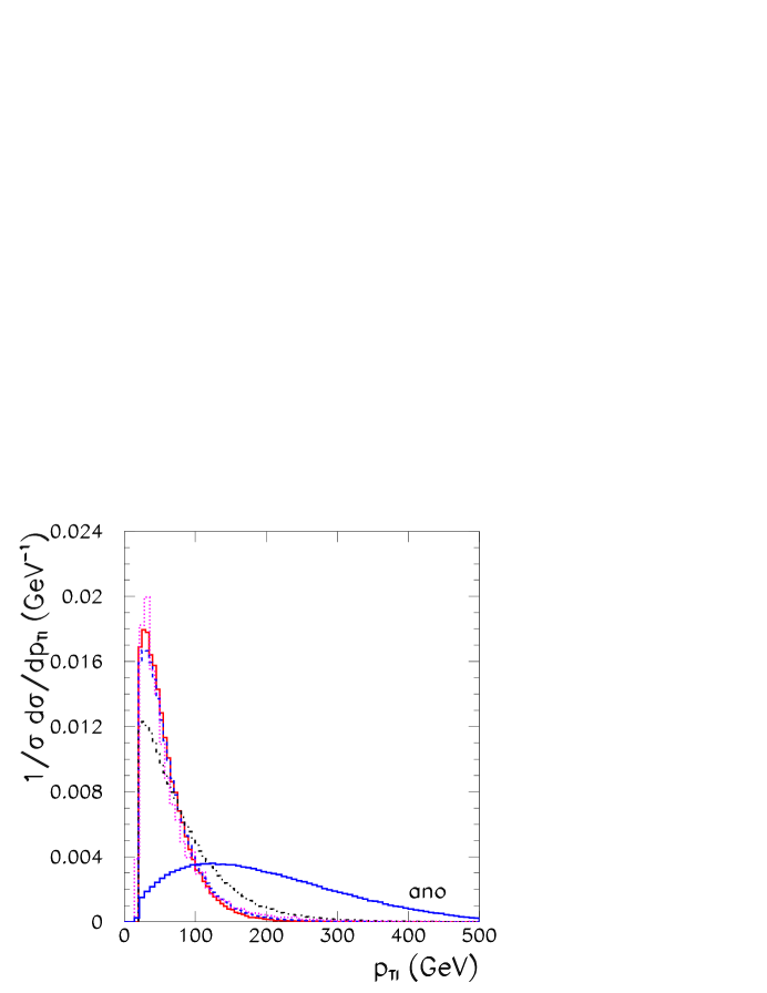
Figure 1: Normalized distribution of the transverse momentum of the charge leptons for $t\bar{t}$ (red solid line), $t\bar{t}j$ (blue dashed line), $t\bar{t}jj$ (black dot-dashed line), SM irreducible production (magenta dotted line), and anomalous $W^{+}W^{-}$ contribution $\sigma_{00}$ (blue solid line marked “ano”). We assumed $m_{h}=120$ GeV and applied cuts (22)–(25) but for with a relaxed cut $p_{T}^{\ell}>20$ GeV.

In order to further reduce these backgrounds we make use of the fact that QCD processes typically occur at smaller invariant masses of tagging jets compared to EW processes. This is illustrated in Fig. 2 where we show the normalized invariant mass distribution of the tagging jets for the different backgrounds and the anomalous contribution $\sigma_{00}$ for $pp\rightarrow jje^{+}\mu^{-}\nu\nu$. Consequently, in order to further suppress the backgrounds we also require a large invariant mass of the tagging jets

$$M_{jj}\geq 1000\hbox{ GeV}\;,$$ (26)

which mainly reduces the $t\bar{t}$ events but still leaves a large background from $t\bar{t}j$ and $t\bar{t}jj$ production. These events can be very efficiently suppressed by vetoing additional soft jet activity in the central region. Consequently, we impose that the event does not contain additional jets with transverse momentum larger than 20 GeV in between the tagging ones,

$$p_{T}^{j}<20~{}\hbox{ GeV}\;\;\;\;\hbox{if}\;\;\;\;\eta_{\rm min}^{j}<\eta_{j}<\eta_{\rm max}^{j}\;.$$ (27)

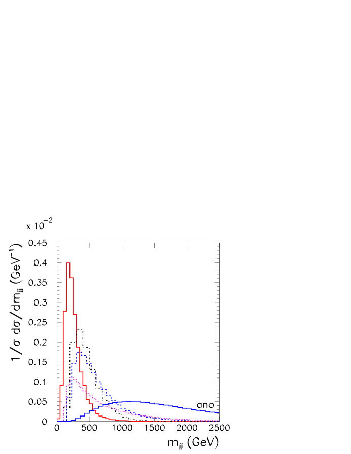
Figure 2: Normalized jet-jet invariant mass distribution for $t\bar{t}$ (red solid line), $t\bar{t}j$ (blue dashed line), $t\bar{t}jj$ (black dot-dashed line), SM irreducible production (magenta dotted line), and anomalous $W^{+}W^{-}$ contribution $\sigma_{00}$ (blue solid line marked “ano”). We assumed $m_{h}=120$ GeV and applied cuts (22)–(25).

Additionally we notice that the azimuthal angular distribution of the charged leptons relative to each other in the SM is different than in the anomalous contributions. The $e^{\pm}\mu^{\mp}$ pairs from the decay of the $W$ pairs produced via the effective interactions (9) and (14) are preferentially emitted in opposite direction from each other. This is shown in Fig. 3 where we plot the normalized distribution of the azimuthal angle between the electron and the muon. Thus we impose also the additional cut

$$\varphi_{e\mu}>2.25\;{\rm rd}.$$ (28)

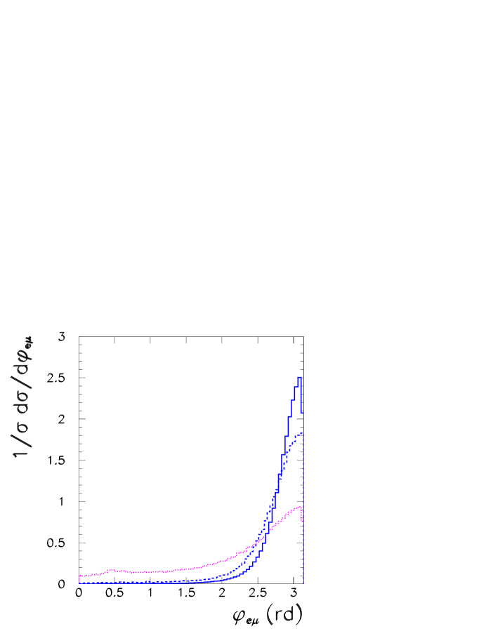
Figure 3: Normalized distribution of the $e\mu$ azimuthal angle difference for $t\bar{t}j$ (dashed line), irreducible background (dotted line), and anomalous $W^{+}W^{-}$ production (solid line). We assumed $m_{h}=120$ GeV and applied cuts (22)–(27).

Finally we make use of the fact that the anomalous contributions arising from the effective interactions (9) and (14) lead to a growth of the cross section for large $WW$ invariant masses; see Fig. 4.

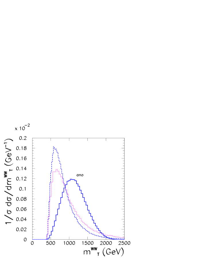
Figure 4: Normalized distribution of $M_{T}^{WW}$ for $t\bar{t}j$ (dashed line), irreducible background (dotted line), and anomalous $W^{+}W^{-}$ production (solid line). We assumed $m_{h}=120$ GeV and applied cuts (22)–(28).

Consequently we define the signal region

$$M_{T}^{WW}\geq 800\hbox{ GeV}\;,$$ (29)

where we define the transverse invariant mass as

$$M_{T}^{WW}=\left(\sqrt{(p_{T}^{e\mu})^{2}+m^{2}_{e\mu}}+\sqrt{/\!\!\!p_{T}^{2}+m^{2}_{e\mu}}\right)^{2}-(\vec{p_{T}^{e\mu}}+\vec{/\!\!\!p_{T}})^{2}$$ (30)

where $\vec{/\!\!\!p_{T}}$ is the missing transverse momentum vector, $\vec{p_{T}^{e\mu}}$ is the transverse momentum of the pair $e$-$\mu$ and $m_{e\mu}$ is the $e\mu$ invariant mass.

In Table 1, we illustrate the effect of the above cuts for $pp\to jje^{\pm}\mu^{\mp}\nu\nu$. In the lines marked IRED$+-$ we take into account the full scattering amplitude for the irreducible backgrounds. We separate the electroweak and QCD part of these backgrounds in order to show the effect of the veto survival probabilities. As illustration of the signal loss due to the imposed cuts, we also include the cross section for the anomalous term $\sigma_{00}$. From this table, we can see that the largest background is the $t\bar{t}+n$ jets production by three order of magnitude when we apply only the acceptance and tagging cuts. However, after cuts the dominant backgrounds are $t\bar{t}j$ and EW irreducible processes.

background/cut	(22)–(25) [$20$ GeV]	(22)–(25)	(22)–(26)	(22)–(27)	(22)–(27) $\times P_{\rm surv}$	(22)–(28) $\times P_{\rm surv}$
IRED$+-$ (QCD)	20.0	1.12	0.26	0.26	0.058	0.035
IRED$+-$ (EW)	4.4	0.30	0.24	0.24	0.14	0.089
$t\bar{t}$	217.	6.96	0.0306	0.0306	0.0069	0.0068
$t\bar{t}j$	1860.	73.8	8.88	0.776	0.175	0.158
$t\bar{t}jj$	682.	77.2	2.21	0.0140	0.0032	0.0031
Anomalous $\sigma_{00}$	2710	1710	1310	1310	786	758

Table 1: Cross sections in fb to illustrate the effect of cuts for the $pp\to jje^{\pm}\mu^{\mp}\nu\nu$ production. The column marked as (22)–(25) [$20$ GeV] shows the total cross sections after applying out basic cuts with a relaxed $p_{T}^{\rm min}=20$ GeV. In computing the SM cross section the contribution from a light Higgs boson with $m_{h}=120$ GeV is included. The cross sections (given in fb) do not include the forward jet and lepton detection efficiencies and they are obtained for choice C1 of the renormalization and factorization scales.

V.3 Cuts for $pp\to jje^{\pm}\mu^{\pm}\nu\nu$

In the first column in Table 2 we give the cross sections for $pp\to jje^{\pm}\mu^{\pm}\nu\nu$ after the basic cuts (22)–(25). As we can see, the only important source of background events is the SM electroweak processes contributing to the same final state.

Further enhancement of the signal from the anomalous contributions can be obtained by studying the transverse momentum of the produced leptons as demonstrated in Fig. 5 which shows the lepton transverse momentum distribution for the anomalous contribution $\sigma_{00}$ and for the SM background. As we can see, the background is peaked toward small lepton transverse momenta while the anomalous contributions leads to the production of leptons with a higher transverse momentum.

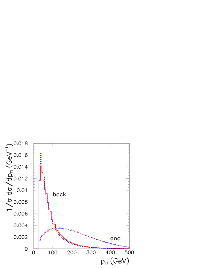
Figure 5: Normalized lepton transverse momentum distribution for IRED$++$ background (solid line), IRED$--$ background (dashed line), $W^{+}W^{+}$ $\sigma_{00}$ (dot-dashed line), and $W^{-}W^{-}$ $\sigma_{00}$ (dotted line). We assumed $m_{h}=120$ GeV and applied cuts (22)–(25).

Consequently, for processes leading to final state leptons with the same charge, we define our signal region by tightening the $p_{T}^{\ell}$ cut

$$p_{T}^{\ell}>100~{}\hbox{GeV.}$$ (31)

background/cut	(22)–(25)	(22)–(25) $+$ (31)	[(22)–(25) $+$ (31)] $\times P_{\rm surv}$
IRED$++$ (QCD)	0.07	0.004	0.0009
IRED$++$ (EW)	1.11	0.105	0.063
Anomalous $\sigma_{00}$	2250.	1470.	880.
IRED$--$ (QCD)	0.025	0.001	0.0002
IRED$--$ (EW)	0.365	0.046	0.028
Anomalous $\sigma_{00}$	536.	334.	200.

Table 2: Effect of cuts for $pp\to jje^{\pm}\mu^{\pm}\nu\nu$ production. The cross sections (in fb) do not include the forward jet and lepton detection efficiencies and they are obtained for choice C1 of the renormalization and factorization scales.

We present in Table 3 our final results for the coefficients $\sigma_{\rm bck},\sigma_{i},\sigma_{i,j}$ of Eq. (20) after cuts (22)–(28) for $pp\rightarrow jje^{\pm}\mu^{\mp}\nu\nu$ and cuts (22)–(25) $+$ (31) for $pp\rightarrow jje^{\pm}\mu^{\pm}\nu\nu$. The results include the effect of the veto survival probabilities as well as the forward jet and lepton detection efficiencies. They were obtained for choice C1 of the renormalization and factorization scales.

scenario	channel	$\sigma_{\rm bck}$	$\sigma_{0}$	$\sigma_{1}$	$\sigma_{00}$	$\sigma_{11}$	$\sigma_{01}$
	$pp\to e^{\pm}\mu^{\mp}\nu\nu jj$	0.067	—	—	300	655	822
$m_{h}=120$ GeV	$pp\to e^{+}\mu^{+}\nu\nu jj$	0.029	$-0.46$	$-0.20$	400	94	380
	$pp\to e^{-}\mu^{-}\nu\nu jj$	0.045	$-0.11$	$-0.04$	91	21	87
	$pp\to e^{\pm}\mu^{\mp}\nu\nu jj$	0.07	1.3	2.1	300	655	822
No light Higgs boson	$pp\to e^{+}\mu^{+}\nu\nu jj$	0.017	$-4.9$	$-2.3$	400	94	380
	$pp\to e^{-}\mu^{-}\nu\nu jj$	0.017	$-1.2$	$-0.54$	91	21	87

Table 3: Cross sections (in fb) for the different terms in Eq. (20). The results include the effect of the veto survival probabilities and the forward jet and lepton detection efficiencies. They are obtained for choice C1 of the renormalization and factorization scales.

V.4 Estimating the Backgrounds

As mentioned above, constraining the quartic gauge boson couplings is essentially a counting experiment and the sensitivity of the search is thus determined by the precision with which the background rate in the search region can be predicted. Since the signal selection is demanding, including double forward jet tagging and central jet vetoing techniques whose acceptance cannot be calculated with sufficient precision in perturbative QCD, the theoretically predicted background can vary up to a large factor. Though the QCD corrections to the irreducible EW processes seem to be modest dieternew the same is not guarantee for the QCD backgrounds. Here the situation is analogous to the Higgs boson production in WBF where the backgrounds must be also estimated from data estback .

We demonstrate the large QCD uncertainties in Fig. 6 where we plot the value of the $t\bar{t}j$ cross section after cuts (22)–(28) for different choices of the factorization and renormalization scale. Moreover, we should also keep in mind that the narrow width approximation used by us has a discrepancy with respect to the full LO amplitude calculation of the order of 10–20% nwafull . The obvious conclusion is that in order to obtain a meaningful estimate of the sensitivity the background levels need to be determined directly from LHC data.

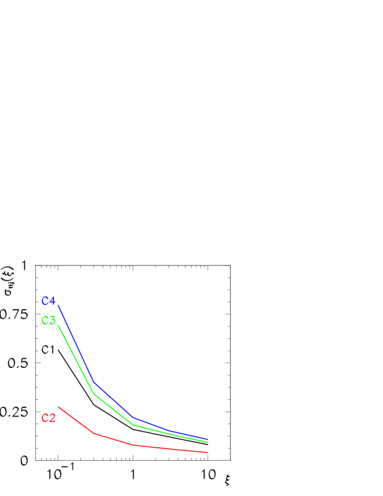
Figure 6: Cross section for $t\bar{t}j$ after cuts (22)–(28) as a function $\xi$, where $\mu_{R}=\xi\mu_{R}^{0}$ for the four choices choices of the factorization and renormalization scale defined in the text.

Fortunately, a sizable sample of $jje^{\pm}\mu^{\mp}\nu\nu$ and $jje^{\pm}\mu^{\pm}\nu\nu$ events will be available if some of the cuts are relaxed. In this way the background normalization error can be reduced by considering a larger phase space region as a calibration region. The background expected in the signal region is then obtained by extrapolation of the measured events in the calibration region to the signal region. This procedure introduces also an uncertainty, which we denote as QCD–extrapolation uncertainty, due to the extrapolation to the signal region. However, as we will show, these uncertainties are smaller than the overall normalization uncertainty.

Using the results in Fig. 4 we see that we can define the calibration region used to estimate the background for $jje^{\pm}\mu^{\mp}\nu\nu$ as the one complying with cuts (22)–(28) and

$$M_{T}^{WW}\leq 800\hbox{ GeV.}$$ (32)

Equivalently from the results in Fig. 5 we find that one can define the calibration region used to estimate the background for $jje^{\pm}\mu^{\pm}\nu\nu$ as the one within cuts (22)–(25)

$$30<p_{T}^{\ell}<100~{}\hbox{GeV.}$$ (33)

As a measure of theoretical uncertainty associated with the extrapolation from the calibration to the signal regions, we study the ratio of the cross sections in the signal region and the calibration region as a function of $\xi$, the scale factor for the four different renormalization scale choices $\mu_{R}=\xi\mu_{R}^{0}$ listed above. In this way we define for the final state exhibiting opposite charge leptons ($jje^{\pm}\mu^{\mp}\nu\nu$)

$$R_{\rm os}=\frac{\displaystyle\sigma_{\rm bck}(M_{T}^{WW}>800\hbox{ GeV})}{\displaystyle\sigma_{\rm bck}(M_{T}^{WW}<800\hbox{ GeV})}\;,$$ (34)

where in the evaluation of these ratios we have added the electroweak and QCD contributions from all background sources taking into account the corresponding veto survival probabilities. On the other hand, for the final state $jje^{\pm}\mu^{\pm}\nu\nu$ that exhibits same charge leptons we define

$$R_{\rm ss}=\frac{\displaystyle\sigma_{\rm bck}(p_{T}^{\ell}>100~{}{\rm GeV})}{\displaystyle\sigma_{\rm bck}(30<p_{T}^{\ell}<100~{}{\rm GeV})}\;,$$ (35)

where we have added the contributions from both signs.

We depict in Fig. 7 the $\xi$ dependence of $R_{\rm os}$ which shows that the extrapolation uncertainty is at a tolerable level ($\simeq 15$%) being much smaller than the normalization uncertainty. The corresponding extrapolation uncertainty for the processes with same sign leptons is smaller by a factor of 2 because of the QCD background is small.

Altogether the total expected uncertainty in the estimated number of background events has two sources: the theoretical uncertainty associated to the extrapolations from the calibration region ($\delta_{\text{bck,th}}$) and the statistical error associated to the determination of the background cross section in the calibration region ($\delta_{\text{bck,stat}}$). This last one is slightly different for the case of light or no light Higgs boson because of the slightly different number of events from the SM irreducible background. Assuming an integrated luminosity of 100 fb^-1 we find

$$\delta_{\text{bck,th,os}}=15\%\;\;,\;\;\; \delta^{\rm lin}_{\text{bck,stat,os}}=34\%\;\;,\;\;\; \delta^{\rm no-lin}_{\text{bck,stat,os}}=31\%\;\;,$$ (36)

$$\delta_{\text{bck,th,ss}}=7.5\%\;\;,\;\;\; \delta^{\rm lin}_{\text{bck,stat,ss}}=22\%\;\;,\;\;\; \delta^{\rm no-lin}_{\text{bck,stat,ss}}=21\%\;\;,$$ (37)

where we denoted by the superscript “lin” (“non-lin”) the case with (without) a light Higgs boson. In addition to these uncertainties considered here there are also experimental systematic uncertainties, which are sizable for the Higgs boson searches estback , however they do require a full detector simulation which is beyond the scope of this work.

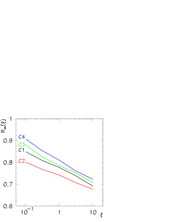
Figure 7: The ratio $R_{\rm os}$ is shown as a function of $\xi$, where $\mu_{R}=\xi\mu_{R}^{0}$ for the four choices of renormalization and factorization scales given in the text.

VI Results and Discussion

In order to obtain the attainable sensitivity to deviations of the SM predictions of the quartic gauge boson couplings we assumed an integrated luminosity of $100$ fb^-1 and that the observed number of events in the different scenarios is compatible with the background expectations for the choice C1 of the renormalization and factorization scales both in the signal ($N^{\text{S}}_{i,\text{data}}$) and in the calibration ($N^{\text{C}}_{i,\text{data}}$) regions, i.e.

$$N^{\text{S}}_{i,\rm data}=N^{\text{S}}_{i,\rm bck,C1}\;\;\;\;\;\hbox{and}\;\;\;\;\;N^{\text{C}}_{i,\rm data}=N^{\text{C}}_{i,\rm bck,C1}\;\;,$$ (38)

where we denote the process $pp\rightarrow jje^{\pm}\mu^{\mp}\nu\nu$ by $i=$ os and the sum of $pp\rightarrow jje^{+}\mu^{+}\nu\nu$ and $pp\rightarrow jje^{-}\mu^{-}\nu\nu$ by $i=$ ss.

Deviations from the SM prediction for the four gauge boson vertices manifest themselves as a difference between the number of observed events and the number of background events estimated from the extrapolation of the background measured in the calibration region ($N_{i,\rm back}^{\text{S}}$), that is,

$$N^{\text{S}}_{i,\rm data}-N_{i,\rm back}^{\text{S}}\;\;,$$ (39)

where $N_{i,\rm back}^{\text{S}}=R_{i}\,N^{\text{C}}_{i,\rm data}$. Notice that (38) implies that we are assuming that no departure of the SM predictions has been observed neither in the control region nor in the signal one.

The statistical error of the number of anomalous events is

$$\sigma_{i,\text{stat}}^{2}=N_{i,\text{data}}^{\text{S}}+(R_{i}\,N_{i,\text{data}}^{\text{C}}\delta_{\text{bck,stat}})^{2}$$ (40)

where the first term is the statistical error of the measured number of events in the signal region and the second term is the error in the determination of the background in the signal region due to the statistical error of the background measurement in the calibration region, $\delta_{\text{bck,stat}}$. The extrapolation uncertainty introduces an additional error

$$\sigma_{i,\text{th}}=R_{i}\,N_{i,\text{data}}^{\text{C}}\delta_{\text{bck,th}}\;\;.$$ (41)

Both errors can be assumed to be Gaussian and we combine then in quadrature.

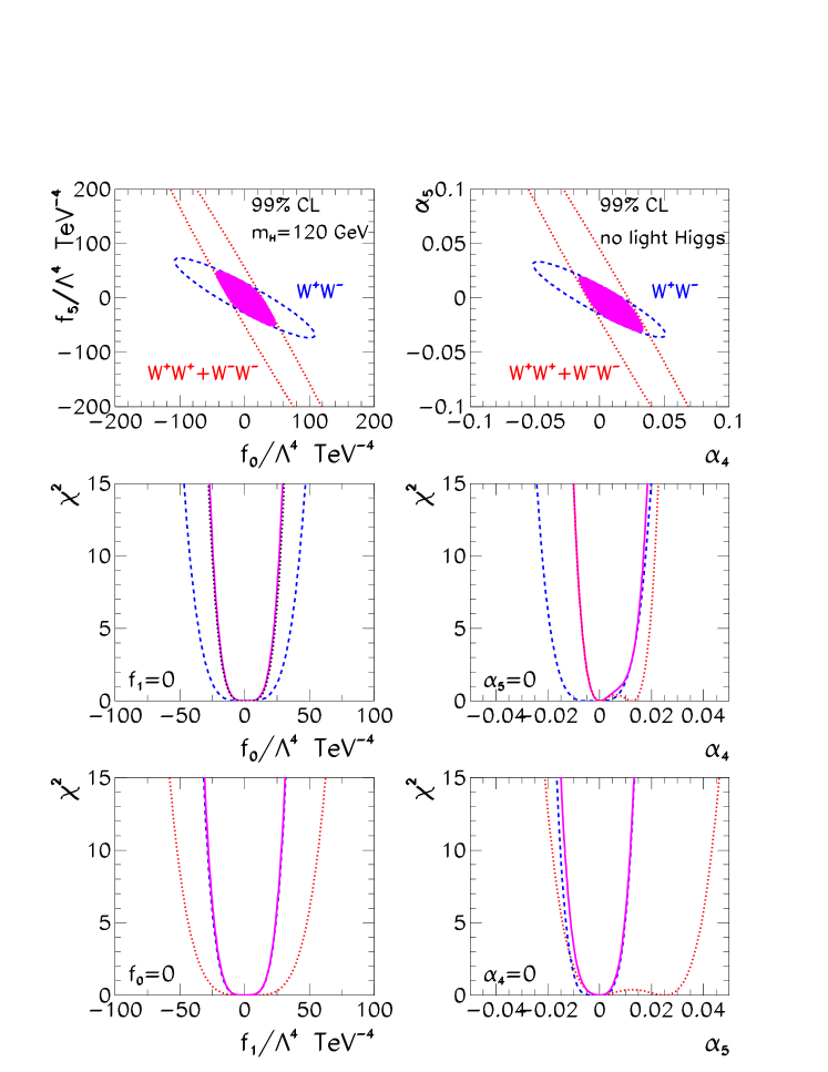
Figure 8: Sensitivity bounds on the coefficients of the anomalous quartic gauge boson operators for the case with a light Higgs boson (left panels) and with no light Higgs boson (right panels). The upper panels show the 99% CL allowed regions for the different channels. The lower panels show the dependence of the $\chi^{2}$ function for the different channels assuming that only under that only one anomalous parameter is non–vanishing. The dashed (dotted) lines corresponds to $pp\rightarrow jje^{\pm}\mu^{\mp}\nu\nu$ ($pp\rightarrow jje^{\pm}\mu^{\pm}\nu\nu$) while the combined analysis is indicated by the filled region and solid lines.

Given our definition of the signal (39), the errors (40)–(41), and the parametrization of the cross section in Eq. (20) we can easily obtain the attainable limits on any combination of quartic anomalous coefficients. We exhibit in the upper panels of Fig. 8 the 99% CL exclusion region in the plane $f_{0}$ versus $f_{1}$ (left) and $\alpha_{4}$ versus $\alpha_{5}$ (right) for each channel $i$ independently, and for the combination of both (full region). As we can see the same sign processes present a very strong correlation between both couplings while the correlation is somewhat smaller for the case of the processes with opposite sign leptons. As a consequence, the final allowed regions are rather “compact” and meaningful sensitivity bounds can be derived.

In the lower panels of Fig. 8 we plot the $\chi^{2}$ as a function of individual couplings, under the assumption that only one anomalous parameter is non–vanishing. From this we find that for the case with a light Higgs boson of $m_{h}=120$ GeV

$$-22< \frac{\displaystyle f_{0}}{\displaystyle\Lambda^{4}}({\rm TeV}^{-4}) <24\;\;,$$ (42)

$$-25< \frac{\displaystyle f_{1}}{\displaystyle\Lambda^{4}}({\rm TeV}^{-4}) <25\;\;,$$ (43)

at 99% CL. In models without a light Higgs boson we get the following 99% CL bounds

$$-7.7\times 10^{-3}< \alpha_{4} <15\times 10^{-3}\;\;,$$ (44)

$$-12\times 10^{-3}< \alpha_{5} <10\times 10^{-3}\;\;.$$ (45)

These results represent an improvement of more than one order of magnitude over the present sensitivity from indirect effects in low energy observables (18) and (19). Notwithstanding, for the case in which a light Higgs boson is found and the gauge theory is linearly realized, they do not reach the expected natural order of magnitude $f_{i}\sim{\cal O}(1)$ for new physics scale above 1 TeV. On the other hand, for scenarios without a light Higgs boson a natural order of magnitude of the anomalous couplings $\alpha_{i}$ in a fundamental gauge theory is $g^{2}v^{2}/\Lambda^{2}$ aew , since the quartic anomalous interactions can be generated by tree diagrams. Thus, we might expect that the size of the $\alpha$’s should be of the order of $M_{Z}^{2}/\Lambda^{2}\simeq 2\times 10^{-3}$ which is close to the attainable sensitivity that we obtain from our analysis.

It is also interesting to notice that the achievable sensitivity at the LHC is close to the recently derived lower bounds based on the usual analytical properties associated with causal, unitary theories grinstein . The lack of observation of an anomalous coupling $\alpha_{4}$ and $\alpha_{5}$ below that bound, would indicate the breakdown of some of these basic properties of the $S$-matrix. In particular, as pointed out in Ref. grinstein , since String theory is designed to produce $S$-matrix with these properties and therefore, the experimental verification of those bounds could be use to falsify string theory.

Acknowledgements: We would like to thank D. Rainwater and N. Kauer for illuminating discussions. This work was partially supported by Fundação de Amparo à Pesquisa do Estado de São Paulo (FAPESP), by Conselho Nacional de Desenvolvimento Científico e Tecnológico (CNPq). MCG-G is supported by National Science Foundation grant PHY-0354776 and by Spanish Grant FPA-2004-00996.

Appendix A Dimension 8 effective operators

We list here the parity conserving effective Lagrangians leading to pure quartic couplings between the weak gauge bosons assuming that a Higgs boson has been discovered, that is, employing the linear representation for the higher order operators. Denoting by $\Phi$ the Higgs doublet and by $U$ an arbitrary $SU(2)_{L}$ transformation, the basic blocks for constructing the effective Lagrangian and their transformations are:

$$\Phi\;,\;\hbox{ that transforms as } \Phi^{\prime}=U\Phi$$ (46)

$$D_{\mu}\Phi\;,\;\hbox{ that transforms as } D^{\prime}_{\mu}\Phi^{\prime}=UD_{\mu}\Phi$$ (47)

$$\hat{W}_{\mu\nu}\equiv\sum_{j}W^{j}_{\mu\nu}\frac{\sigma^{j}}{2}\;,\;\hbox{ that transforms as } \hat{W}_{\mu\nu}^{\prime}=U\hat{W}_{\mu\nu}U^{\dagger}$$ (48)

$$B_{\mu\nu}\;,\;\hbox{ that transforms as } B_{\mu\nu}^{\prime}=B_{\mu\nu}$$ (49)

where $W^{i}_{\mu\nu}$ is the $SU(2)_{L}$ field strength and $B_{\mu\nu}$ is the $U(1)_{Y}$ one. The covariant derivative is given by $D_{\mu}\Phi=(\partial_{\mu}-igW^{j}_{\mu}\frac{\sigma^{j}}{2}-ig^{\prime}B_{\mu}\frac{1}{2})\Phi$.

The lowest dimension operator that leads to quartic interactions but does not exhibit two or three weak gauge boson vertices is dimension 8. The counting is straight foward: when can get a weak boson field either from the covariant derivative of $\Phi$ or from the field strength tensor. In either case the vector field is accompanied by a VEV or a derivative. Therefore genuine quartic vertices are of dimension 8 or higher.

There are three classes of such operators:

A.0.1 Operators containing just $D_{\mu}\Phi$

The two independent operators in this class are

$${\cal L}_{S,0} = \left[\left(D_{\mu}\Phi\right)^{\dagger}D_{\nu}\Phi\right]\times\left[\left(D^{\mu}\Phi\right)^{\dagger}D^{\nu}\Phi\right]$$ (50)

$${\cal L}_{S,1} = \left[\left(D_{\mu}\Phi\right)^{\dagger}D^{\mu}\Phi\right]\times\left[\left(D_{\nu}\Phi\right)^{\dagger}D^{\nu}\Phi\right]$$ (51)

A.0.2 Operators containing $D_{\mu}\Phi$ and field strength

The operators in this class are:

$${\cal L}_{M,0} = \hbox{Tr}\left[\hat{W}_{\mu\nu}\hat{W}^{\mu\nu}\right]\times\left[\left(D_{\beta}\Phi\right)^{\dagger}D^{\beta}\Phi\right]$$ (52)

$${\cal L}_{M,1} = \hbox{Tr}\left[\hat{W}_{\mu\nu}\hat{W}^{\nu\beta}\right]\times\left[\left(D_{\beta}\Phi\right)^{\dagger}D^{\mu}\Phi\right]$$ (53)

$${\cal L}_{M,2} = \left[B_{\mu\nu}B^{\mu\nu}\right]\times\left[\left(D_{\beta}\Phi\right)^{\dagger}D^{\beta}\Phi\right]$$ (54)

$${\cal L}_{M,3} = \left[B_{\mu\nu}B^{\nu\beta}\right]\times\left[\left(D_{\beta}\Phi\right)^{\dagger}D^{\mu}\Phi\right]$$ (55)

$${\cal L}_{M,4} = \left[\left(D_{\mu}\Phi\right)^{\dagger}\hat{W}_{\beta\nu}D^{\mu}\Phi\right]\times B^{\beta\nu}$$ (56)

$${\cal L}_{M,5} = \left[\left(D_{\mu}\Phi\right)^{\dagger}\hat{W}_{\beta\nu}D^{\nu}\Phi\right]\times B^{\beta\mu}$$ (57)

$${\cal L}_{M,6} = \left[\left(D_{\mu}\Phi\right)^{\dagger}\hat{W}_{\beta\nu}\hat{W}^{\beta\nu}D^{\mu}\Phi\right]$$ (58)

$${\cal L}_{M,7} = \left[\left(D_{\mu}\Phi\right)^{\dagger}\hat{W}_{\beta\nu}\hat{W}^{\beta\mu}D^{\nu}\Phi\right]$$ (59)

A.0.3 Operators containing just the field strength tensor

The following operators containing just the field strength tensor also lead to quartic anomalous couplings:

$${\cal L}_{T,0} = \hbox{Tr}\left[\hat{W}_{\mu\nu}\hat{W}^{\mu\nu}\right]\times\hbox{Tr}\left[\hat{W}_{\alpha\beta}\hat{W}^{\alpha\beta}\right]$$ (60)

$${\cal L}_{T,1} = \hbox{Tr}\left[\hat{W}_{\alpha\nu}\hat{W}^{\mu\beta}\right]\times\hbox{Tr}\left[\hat{W}_{\mu\beta}\hat{W}^{\alpha\nu}\right]$$ (61)

$${\cal L}_{T,2} = \hbox{Tr}\left[\hat{W}_{\alpha\mu}\hat{W}^{\mu\beta}\right]\times\hbox{Tr}\left[\hat{W}_{\beta\nu}\hat{W}^{\nu\alpha}\right]$$ (62)

$${\cal L}_{T,3} = \hbox{Tr}\left[\hat{W}_{\alpha\mu}\hat{W}^{\mu\beta}\hat{W}^{\nu\alpha}\right]\times B_{\beta\nu}$$ (63)

$${\cal L}_{T,4} = \hbox{Tr}\left[\hat{W}_{\alpha\mu}\hat{W}^{\alpha\mu}\hat{W}^{\beta\nu}\right]\times B_{\beta\nu}$$ (64)

$${\cal L}_{T,5} = \hbox{Tr}\left[\hat{W}_{\mu\nu}\hat{W}^{\mu\nu}\right]\times B_{\alpha\beta}B^{\alpha\beta}$$ (65)

$${\cal L}_{T,6} = \hbox{Tr}\left[\hat{W}_{\alpha\nu}\hat{W}^{\mu\beta}\right]\times B_{\mu\beta}B^{\alpha\nu}$$ (66)

$${\cal L}_{T,7} = \hbox{Tr}\left[\hat{W}_{\alpha\mu}\hat{W}^{\mu\beta}\right]\times B_{\beta\nu}B^{\nu\alpha}$$ (67)

$${\cal L}_{T,8} = B_{\mu\nu}B^{\mu\nu}B_{\alpha\beta}B^{\alpha\beta}$$ (68)

$${\cal L}_{T,9} = B_{\alpha\mu}B^{\mu\beta}B_{\beta\nu}B^{\nu\alpha}$$ (69)

References

- (1) For a review see H. Aihara et al., in Electroweak Symmetry Breaking and New Physics at the TeV Scale, edited by T. Barklow, S. Dawson, H. Haber and J. Seigrist, (World Scientific, Singapore, 1996), p. 488 [arXiv:hep-ph/9503425].
- (2) P. Achard et al. [L3 Collaboration], Phys. Lett. B 586, 151 (2004); P. Abreu et al. [DELPHI Collaboration], Phys. Lett. B 502, 9 (2001); S. Schael et al. [ALEPH Collaboration], Phys. Lett. B 614 (2005) 7; G. Abbiendi et al. [OPAL Collaboration], Eur. Phys. J. C 33, 463 (2004).
- (3) ALEPH, DELPHI, L3, OPAL and the LEP Electroweak Working Group, arXiv:hep-ex/0511027.
- (4) K. Gounder [CDF Collaboration], arXiv:hep-ex/9903038; B. Abbott et al. [DØ Collaboration], Phys. Rev. D 62, 052005 (2000).
- (5) C. Arzt, M. B. Einhorn and J. Wudka, Nucl. Phys. B433, 41 (1995).
- (6) O. J. P. Éboli, M. C. Gonzalez-Garcia, S. M. Lietti and S. F. Novaes, Phys. Rev. D 63, 075008 (2001).
- (7) P. J. Dervan, A. Signer, W. J. Stirling and A. Werthenbach , J. Phys. G26, 607 (2000).
- (8) O. J. P. Éboli, M. C. Gonzalez-Garcia and S. M. Lietti, Phys. Rev. D 69, 095005 (2004).
- (9) G. Belanger, F. Boudjema, Y. Kurihara, D. Perret-Gallix and A. Semenov, Eur. Phys. J. C 13, 283 (2000).
- (10) G. Bélanger and F. Boudjema, Phys. Lett. B 288, 201 (1992); W. J. Stirling and A. Werthenbach, Eur. Phys. J. C 14, 103 (2000).
- (11) G. Bélanger and F. Boudjema, Phys. Lett. B 288, 210 (1992).
- (12) O. J. P. Éboli, M. B. Magro, P. G. Mercadante and S. F. Novaes, Phys. Rev. D 52, 15 (1995).
- (13) O. J. P. Éboli, M. C. Gonzalez-Garcia, and S. F. Novaes, Nucl. Phys. B411, 381 (1994).
- (14) J. Bagger, S. Dawson and G. Valencia, Nucl. Phys. B399, 364 (1993).
- (15) J. Bagger et al., Phys. Rev. D 49, 1246 (1994); Phys. Rev. D 52, 3878 (1995).
- (16) A. Dobado, D. Espriu and M. J. Herrero, Z. Phys. C 50, 205 (1991); A. Dobado and M. T. Urdiales, Z. Phys. C 17, 965 (1996); A. Dobado, M. J. Herrero, E. Ruiz, M. T. Urdiales and R. Pelaez, Phys. Lett. B 352, 400 (1995).
- (17) A. S. Belyaev, O. J. P. Éboli, M. C. Gonzalez-Garcia, J. K. Mizukoshi, S. F. Novaes and I. Zacharov, Phys. Rev. D 59, 015022 (1999).
- (18) J. M. Cornwall, D. N. Levin and G. Tiktopoulos, Phys. Rev. D 10, 1145 (1974); C. E. Vayonakis, Lett. Nuovo Cim. 17, 383 (1976); B. W. Lee, C. Quigg and H. B. Thacker, Phys. Rev. D 16, 1519 (1977); M. S. Chanowitz and M. K. Gaillard, Nucl. Phys. B261, 379 (1985).
- (19) G. L. Kane, W. W. Repko and W. B. Rolnick, Phys. Lett. B 148, 367 (1984); S. Dawson, Nucl. Phys. B249, 42 (1985).
- (20) B. Lee, C. Quigg and H. Thacker, Phys. Rev. Lett. 38, 883 (1977); Phys. Rev. D 16, 1519 (1977); D. Dicus and V. Mathur, Phys. Rev. D 7, 3111 (1973).
- (21) R. Barbieri, A. Pomarol, R. Rattazzi and A. Strumia, Nucl. Phys. B703, 127 (2004).
- (22) A. Brunstein, O. J. P. Éboli and M. C. Gonzalez-Garcia, Phys. Lett. B 375, 233 (1996).
- (23) W. Buchmüller and D. Wyler, Nucl. Phys. B268, 621 (1986); C. J. C. Burges and H. J. Schnitzer, Nucl. Phys. B228, 454 (1983); C. N. Leung, S. T. Love and S. Rao, Z. Phys. C 31, 433 (1986); A. De Rújula, M. B. Gavela, P. Hernández and E. Massó, Nucl. Phys. B384, 3 (1992); K. Hagiwara, S. Ishihara, R. Szalapski and D. Zeppenfeld, Phys. Lett. B 283, 353 (1992); Phys. Rev. D 48, 2182 (1993).
- (24) T. Appelquist and C. Bernard, Phys. Rev. D 22, 200 (1980); A. Longhitano, Phys. Rev. D 22, 1166 (1980); Nucl. Phys. B188, 118 (1981).
- (25) M. S. Chanowitz, M. Golden and H. Georgi, Phys. Rev. D 36, 1490 (1987).
- (26) G. Altarelli and R. Barbieri, Phys. Lett. B 253, 161 (1991); G. Altarelli, R. Barbieri and S. Jadach, Nucl. Phys. B369, 3 (1992) [Erratum-ibid. B376, 444 (1992)].
- (27) M. E. Peskin and T. Takeuchi, Phys. Rev. D 46, 381 (1992).
- (28) T. Stelzer and W. F. Long, Comput. Phys. Commun. 81, 357 (1994).
- (29) H. Murayama, I. Watanabe and K. Hagiwara, KEK report 91-11 (unpublished).
- (30) A. Denner, S. Dittmaier, M. Roth and D. Wackeroth, Nucl. Phys. B 560, 33 (1999).
- (31) C. Oleari and D. Zeppenfeld, Phys. Rev. D 69, 093004 (2004).
- (32) B. Jager, C. Oleari and D. Zeppenfeld, arXiv:hep-ph/0604200; B. Jager, C. Oleari and D. Zeppenfeld, arXiv:hep-ph/0603177.
- (33) H. L. Lai et al. [CTEQ Collaboration], Eur. Phys. J. C 12, 375 (2000).
- (34) E. E. Boos, H. J. He , W. Kilian, A. Pukhov and P. M. Zerwas, Phys. Rev. D 57, 1553 (1997).
- (35) V. Barger et al., Phys. Rev. D 42, 3052 (1990).
- (36) V. Barger, R. Phillips and D. Zeppenfeld, Phys. Lett. B 346, 106 (1995).
- (37) H. Chehime and D. Zeppenfeld, Phys. Rev. D 47, 3898 (1993); D. Rainwater, R. Szalapski and D. Zeppenfeld, Phys. Rev. D 54, 6680 (1996).
- (38) D. Rainwater, Ph.D. thesis, report arXiv:hep-ph/9908378.
- (39) V. Cavasinni, D. Costanzo and I. Vivarelli, ATL-PHYS-2002-008; S. Asai et al., Eur. Phys. J. C 32S2, 19 (2004).
- (40) D. L. Rainwater and D. Zeppenfeld, Phys. Rev. D 60, 113004 (1999) [Erratum-ibid. D 61, 099901 (2000)]; N. Kauer, T. Plehn, D. L. Rainwater and D. Zeppenfeld, Phys. Lett. B 503, 113 (2001).
- (41) See, for instance, N. Kauer, Phys. Rev. D 70, 014020 (2004); C. Buttar et al., arXiv:hep-ph/0604120; O. J. P. Éboli and D. Zeppenfeld, Phys. Lett. B 495, 147 (2000).
- (42) N. Kauer, Phys. Rev. D 67, 054013 (2003); N. Kauer and D. Zeppenfeld, Phys. Rev. D 65, 014021 (2002).
- (43) J. Distler, B. Grinstein and I. Z. Rothstein, arXiv:hep-ph/0604255.