CERN-PH-TH/2006-105

Living Dangerously with Low-Energy Supersymmetry

Gian F. Giudice and Riccardo Rattazzi

CERN, Theory Division, CERN, CH-1211 Geneva 23, Switzerland

We stress that the lack of direct evidence for supersymmetry forces the soft mass parameters to lie very close to the critical line separating the broken and unbroken phases of the electroweak gauge symmetry. We argue that the level of criticality, or fine-tuning, that is needed to escape the present collider bounds can be quantitatively accounted for by assuming that the overall scale of the soft terms is an environmental quantity. Under fairly general assumptions, vacuum-selection considerations force a little hierarchy in the ratio between $m_{Z}^{2}$ and the supersymmetric particle square masses, with a most probable value equal to a one-loop factor.

1 Introduction

For almost three decades, the gauge hierarchy problem has been the only reason to think that the Standard Model (SM) should be overthrown right around the weak scale. It has inspired the construction of a huge stack of new models and is arguably one of the main motivation to build the Large Hadron Collider. As it is normally formulated, the problem lies in the difficulty to understand the relatively low value of the Higgs mass parameter $|m_{H}^{2}|\sim(100\,\mathrm{GeV})^{2}$ in a framework in which the SM is valid up to some ultra-high scale $\Lambda$, for instance for $\Lambda$ of the order of the Planck scale $M_{P}$. We can equivalently picture the problem as one of criticality. Imagine the fundamental theory at the Planck scale has a few free parameters. In string theory, to be perhaps more concrete, these parameters may correspond to the (discrete) set of vacuum expectation values of the moduli fields. Let us consider the phase diagram for electroweak symmetry breaking, in the space of these parameters. Over the bulk of the parameter space, $|m_{H}^{2}|$ is expected to be of order $M_{P}^{2}$, and therefore either $\langle H\rangle\sim M_{P}$ or $\langle H\rangle=0$ depending on the sign of $m_{H}^{2}$. The hierarchy problem is now simply stated as: if the critical line separating the two phases is not special from the point of view of the fundamental theory, why are the parameters in the real world so chosen as to lie practically atop the critical line?

Supersymmetry is relevant to this puzzle for two reasons. First, because it selects the critical line as a locus of enhanced symmetry. More precisely, in the minimal supersymmetric SM with both supersymmetry and Peccei-Quinn (PQ) symmetry unbroken, the Higgs potential $V\propto(|H_{1}|^{2}-|H_{2}|^{2})^{2}$ is indeed “critical”, in the sense that the symmetric $H_{1}=H_{2}=0$ point is a minimum of the potential, but it can be destabilized by arbitrarily small mass perturbations. Second, supersymmetry is, under rather general circumstances, broken only by tiny non-perturbative effects [1]. These will unavoidably move the theory slightly off the critical line. Effectively this corresponds to the generation of tiny mass terms $\sim M_{P}e^{-1/\alpha}\ll M_{P}$ which generically lead to electroweak symmetry breakdown (while stabilizing at the same time the flat direction $|H_{1}|=|H_{2}|$) at a correspondingly low scale.

In hidden sector models, at energies below the Planck mass $M_{P}$, supersymmetry breaking is accurately parametrized by soft supersymmetry-breaking terms of order $M_{S}$. The electroweak vacuum dynamics is then controlled by Renormalization-Group (RG) evolution of the soft terms from $M_{P}$ down to $M_{S}$. One nice feature of this evolution is that, over a wide region of the soft parameter space, one of the eigenvalues of the Higgs squared-mass matrix flows to a negative value somewhere between $M_{P}$ and $M_{S}$ [2]. This makes electroweak symmetry breaking a rather natural phenomenon within supersymmetric extensions of the SM.

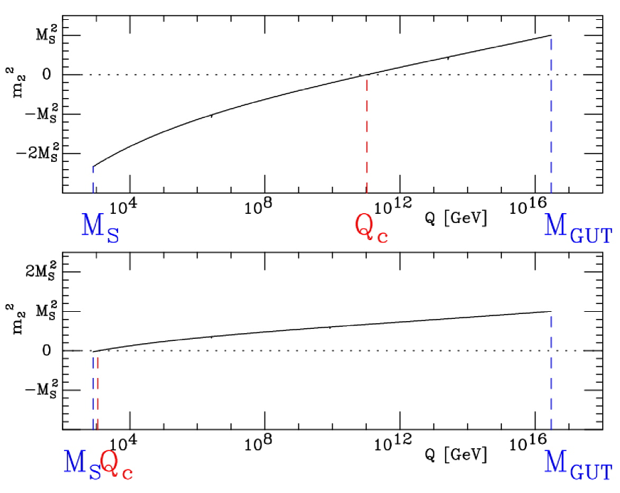
Figure 1: The running of the Higgs mass parameter $m_{2}^{2}$ as a function of the RG scale $Q$. The top frame shows the case of a generic supersymmetric setup, leading to $|m_{2}^{2}(M_{S})|=O(M_{S}^{2})$ and $M_{S}\ll Q_{c}\ll M_{P}$. The bottom frame corresponds to a fine-tuned choice of soft terms, such that $|m_{2}^{2}(M_{S})|\ll M_{S}^{2}$ and $M_{S}\simeq Q_{c}$.

For the sake of this discussion we should, however, be slightly more precise. Notice that, since the RG evolution is homogeneous in the soft terms, the RG scale $Q_{c}$ at which the Higgs mass eigenvalue crosses zero depends on $M_{P}$ and on dimensionless ratios of soft parameters, but it is parametrically unrelated to $M_{S}$. Furthermore, as long as the Higgs mass matrix is positive definite at $M_{P}$, since the evolution is logarithmic in the RG scale, $Q_{c}$ is exponentially suppressed with respect to $M_{P}$ (see fig. 1, top frame). Therefore, the supersymmetric parameter space is essentially divided into two regions (phases) characterized respectively by $M_{S}\ll Q_{c}\ll M_{P}$ and $Q_{c}\ll M_{S}\ll M_{P}$. In the first region, at the scale $M_{S}$ where RG evolution of the soft terms is frozen, the Higgs mass matrix has a negative eigenvalue of magnitude $\sim M_{S}^{2}$, due to the hierarchical separation between $M_{S}$ and $Q_{c}$. Given the structure and size of the Higgs quartic potential, this implies a weak scale $\langle H\rangle^{2}\sim M_{S}^{2}/g^{2}$ and $m_{Z}^{2}\sim M_{S}^{2}$. In the second region, RG evolution is frozen with a positive definite Higgs mass matrix so that the Higgs field does not break electroweak symmetry. We call this region the unbroken phase, although electroweak symmetry is still spontaneoulsly broken, but only by fermion condensation in QCD. The resulting spectrum is therefore vastly different than in the $\langle H\rangle\sim M_{S}/g$ phase. All elementary SM particles, including $W$ and $Z$, weigh less than about 100 MeV, while the superparners are still at $M_{S}$, so that the pattern is $m_{Z}<\Lambda_{\rm QCD}\ll M_{S}$. While the unbroken phase region does not resemble even approximately the world we live in, the broken phase region makes instead supersymmetry relevant to phenomenology, as it solves the gauge hierarchy problem and explains electroweak symmetry breaking in a unitary conceptual framework.

The generic spectrum $M_{S}\sim m_{Z}$ of the broken phase also held up great expectations for a discovery of supersymmetry at LEP [3]. As those expectations were then frustrated by the experimental data, in the post-LEP era also the broken phase does not seem to qualitatively describe our world. The direct and indirect limits placed by LEP point instead to a spectrum where $M_{S}$ is at least an order of magnitude larger than $m_{Z}(\gg\Lambda_{\rm QCD})$, corresponding to the boundary between the two phases. The strongest, but not unique, constraint is given by the experimental lower limit on the mass of the lightest CP-even Higgs $m_{h}$. Given the tree-level theoretical upper bound $m_{h}<m_{Z}|\cos 2\beta|$, the experimental constraint can be satisfied only by pumping up the top-stop quantum corrections to the Higgs quartic coupling [4]. Over most of the parameter space, this implies stop masses $m_{\tilde{t}}$ that range closer to a TeV than to 100 GeV. We can then work out where $Q_{c}$ should be, by expanding the RG evolution of the negative mass eigenvalue in the Higgs potential between $Q_{c}$ and $M_{S}$. For the sake of the argument we can focus on the case $\tan\beta\to\infty$, where electroweak breaking is driven by the Higgs mass parameter $m_{2}^{2}$ and where we find

$$\frac{m_{Z}^{2}}{2}=-m_{2}^{2}\simeq\left.\frac{dm_{2}^{2}}{d\ln Q}\right|_{Q_{c}}\ln\frac{Q_{c}}{M_{S}}.$$ (1)

For typical choices of supersymmetric parameters, the stop masses dominate the RG evolution and $dm_{2}^{2}/d\ln Q\simeq 0.1m_{\tilde{t}}^{2}$. For $m_{\tilde{t}}\sim 1$ TeV, we find $\ln(Q_{c}/M_{S})<1$, which is so small that there is not even a meaningful scale separation between the overall supersymmetric scale $M_{S}$ and $Q_{c}$ (see fig. 1, bottom frame). The coincidence of these two conceptually unrelated mass scales is one way of viewing the fine-tuning problem of supersymmetric models. Why should the fundamental theory prefer such critical choice of parameters? A more quantitative illustration of this question will be given in the next section and the rest of the paper is an attempt to provide an answer.

2 Fine-Tuning and Criticality in Low-Energy Supersymmetry

In this section, we want to explain, in a more quantitative fashion, the connection between fine tuning and criticality. Let us consider the phase diagram in the parameter space of the minimal supersymmetric model, spanned by all independent dimensionless ratios of the coefficients of soft supersymmetry-breaking terms. For illustrative purposes, we reduce this multi-dimensional space into a plane, by taking unified gaugino masses ($M$) and universal scalar masses ($m^{2}$) at the GUT scale. For the moment, we also set to zero all trilinear soft terms at the GUT scale ($A=0$), and choose a small bilinear term $B$ at the scale $M_{S}$, corresponding to a fixed and moderately large value of $\tan\beta$, in the region where radiative electroweak breaking occurs. These hypotheses are just meant to simplify the visualization, but the discussion we present here remains valid also for general soft terms. In the case under consideration, the phase diagram can be described in terms of only two variables, which we take to be $m^{2}/\mu^{2}$ and $M^{2}/\mu^{2}$, the square ratios of the common scalar and gaugino masses to the $\mu$ parameter, with all quantities defined at the GUT scale.

The SM presents two phases, with broken ($\langle H\rangle\neq 0$) or unbroken ($\langle H\rangle=0$) electroweak symmetry. The situation is more complicated in the supersymmetric version, because of the extended structure of the Higgs sector and of the properties of supersymmetry. We recall that the Higgs potential, along the neutral field components is

$$V=\frac{g^{2}+g^{\prime 2}}{8}\left(|H_{1}|^{2}-|H_{2}|^{2}\right)^{2}+m_{1}^{2}|H_{1}|^{2}+m_{2}^{2}|H_{2}|^{2}-m_{3}^{2}\left(H_{1}H_{2}+{\rm h.c.}\right),$$ (2)

and that we are working in the limit of small $m_{3}^{2}$. The boundary condition at the GUT scale is $m_{1,2}^{2}=m^{2}+\mu^{2}$.

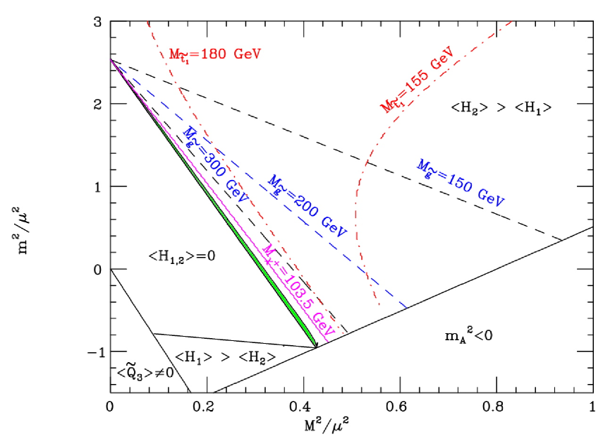
Figure 2: The phase diagram of the minimal supersymmetric SM, assuming a universal scalar mass $m^{2}$, a gaugino unified mass $M$, a Higgsino mass $\mu$, and trilinear term $A=0$, with all parameters defined at the GUT scale. The top Yukawa coupling is fixed such that $m_{t}=172.7$ GeV and $\tan\beta=10$ in the usual phase with electroweak breaking. Some contours are shown for masses of the lightest stop ($M_{{\tilde{t}}_{1}}$), the gluino ($M_{\tilde{g}}$), and the lightest chargino ($M_{\chi^{+}}$). The green (gray) area shows the region of parameters allowed after LEP Higgs searches.

The phase diagram of the minimal supersymmetric SM is shown in fig. 2. A first peculiarity of supersymmetry is the existence of phases where color and electric charge are broken. This happens, for instance, at negative $m^{2}$ and small $M$, where the third-generation squark $\tilde{Q}_{3}$ gets a vacuum expectation value. Actually, assuming strict universality, there is an even larger region where the selectron gets a vacuum expectation value, which is not shown in fig. 2 since, for the sake of argument, we take a common scalar mass only for the particles involved in the conventional $SU(2)\times U(1)$ breaking pattern (third-generation squarks and the two Higgses).

More interesting is a special multi-critical point, separating the various Higgs phases, that corresponds to vanishing Higgs bilinear terms ($m_{1}^{2}=m_{2}^{2}=m_{3}^{2}=0$). This point, which is actually a surface in the case of general soft terms, occurs at negative $m^{2}$, in the example we are considering. Moving away from the multi-critical point, different phases emerge, depending on the signs and the values of $m_{1}^{2}$ and $m_{2}^{2}$ at the scale $M_{S}$. For positive $m_{1,2}^{2}$, the potential is stabilized at the origin; the scale $M_{S}$ is larger than the critical scale $Q_{c}$, and electroweak symmetry is unbroken. Notice that this phase (marked as $\langle H_{1,2}\rangle=0$ in fig. 2) extends, for $M=0$, to rather large values of $m^{2}/\mu^{2}$. This is a peculiarity of the assumption of strict universality which, together with the known value of the top mass, leads to a certain cancellation of the contribution to $m_{Z}^{2}$ proportional to $m^{2}$. Varying the top Yukawa coupling (or, ultimately, $\tan\beta$), one can obtain higher degrees of cancellation, approaching what is known as “focus point” [5]. To compensate for this reduced dependence on $m^{2}$ (a characteristic of universality, not shared by generic soft-term structures) we have expanded in fig. 2 the scale of the vertical axis, with respect to the horizontal axis. For the same reason, the precise location of the boundary between the broken and unbroken phases at small $M$ sensitively depends on the values of the coupling constants and on the degree of accuracy of the calculation. In our figures, we have chosen $\alpha_{s}(m_{Z})=0.1176$, and fixed the top Yukawa coupling corresponding to $m_{t}=172.7$ GeV and $\tan\beta=10$ in the broken phase. We have also limited our RG evolution to one-loop approximation.

In the limit of exact supersymmetry and PQ symmetry, all quadratic Higgs terms in eq. (2) vanish. Actually, since in supergravity scenarios the PQ breaking can easily arise only from supersymmetry breaking [6], we will refer to this case ($m_{1,2,3}^{2}=0$) as the supersymmetric limit. In this limit, the Higgs potential has a flat direction $\langle H_{1}\rangle=\langle H_{2}\rangle$, characteristic of supersymmetric $D$-terms. Supersymmetry breaking stabilizes this direction as long as $m_{1}^{2}+m_{2}^{2}>2|m_{3}^{2}|$. If this is not the case, the Higgs field slides up to the renormalization scale where the previous inequality is satisfied, as in the Coleman-Weinberg mechanism. If $m^{2}/\mu^{2}<-1$, this scale is actually larger than the GUT scale cutoff. At any rate, the important point is that the Higgs vacuum expectation value is unrelated to the supersymmetry scale $M_{S}$ and in particular $m_{Z}\ll M_{S}$. This region, which is of course experimentally ruled out is marked in fig. 2 by $m_{A}^{2}<0$. Indeed, its boundary is characterized, in our analysis with fixed $\tan\beta$, by the condition $m_{A}\equiv m_{1}^{2}+m_{2}^{2}<0$ since, in the region of conventional electroweak breaking, $2m_{3}^{2}=\sin 2\beta(m_{1}^{2}+m_{2}^{2})$.

In the rest of the phase diagram in fig. 2 the Higgs vacuum expectation value is proportional to supersymmetry-breaking terms, and therefore $M_{S}$ controls the size of electroweak breaking, thus providing a potentially realistic solution to the hierarchy problem. Depending on whether $m_{1}^{2}$ or $m_{2}^{2}$ is driven negative, we obtain two possible regions marked in fig. 2 as $\langle H_{1}\rangle>\langle H_{2}\rangle$ and $\langle H_{2}\rangle>\langle H_{1}\rangle$, respectively. The first region, which occurs only at negative $m^{2}$, has phenomenological difficulties in maintaining a perturbative top Yukawa coupling to large scales and in making the Higgs mass sufficiently heavy. Therefore, we will concentrate on the region with $\langle H_{2}\rangle>\langle H_{1}\rangle$.

In this region, the inequality $Q_{c}>M_{S}$ is satisfied, and we can determine the overall mass scale of supersymmetric particles from the condition that radiative electroweak breaking reproduces the known value of $m_{Z}$. The complete mass spectrum can then by computed at a given point of the phase diagram, and in fig. 2 we show some characteristic values of supersymmetric particle masses. In the bulk of the region, we find that supersymmetric colored particles weigh typically less than 2–3 times $m_{Z}$, while some electroweak particles are lighter than $m_{Z}$. The values of the supersymmetric masses have only mild variations in the bulk of the region, but they precipitously increase in the proximity of the critical line separating the broken and unbroken phases, where the critical scale $Q_{c}$ rapidly approaches $M_{S}$. Only near the boundary we can find supersymmetric masses compatible with the present bounds from collider experiments. For instance, the chargino-mass LEP bound $M_{\chi^{+}}>103.5$ GeV at 95 % CL [7] rules out all the region to the right of the corresponding blue line in fig. 2, allowing only the narrow strip between the blue and critical lines. Actually the negative Higgs searches impose even stronger constraints on the allowed region. Taking into account the limits on Higgs production at LEP [8] in the channels $Zh$, $ZH$, $hA$, $HA$ (where $h$, $H$, $A$ are the three neutral supersymmetric Higgses), we find that the only allowed points in fig. 2 are those inside the green (gray) region, clustering along the critical line.

A first conclusion that we can draw from these results is that the most natural prediction of supersymmetry on the spectrum of new particles has already been ruled out, and only small corners of parameter space are still allowed. This conclusion is of course well known and it has been already quantified in different ways [3, 9]. Figure 2 presents an alternative way to illustrate the problem.

However, fig. 2 also leads us to a new way of characterizing the allowed region, in terms of criticality condition. The problem of understanding why supersymmetry may have chosen highly untypical values of soft parameters, which appear to have the only effect to hide it from collider searches, is now turned into the question of why supersymmetry wants to lie in a near-critical condition. In the following, we will discuss possible statistical (or dynamical) attempts to explain this puzzle. But before ending this section, we want to address the question of how general is our conclusion that the only allowed parameter region of low-energy supersymmetry lies close to the critical line, and we investigate if other regions, albeit tuned, can arise far from it.

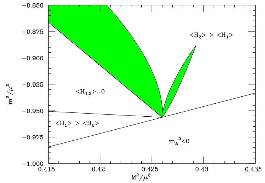
Figure 3: Same as fig. 2, zooming in the allowed region where the Higgs pseudoscalar mass is close to $m_{Z}$.

It is well known that the experimental SM Higgs mass bound $m_{h}>114.4$ GeV at 95% CL [10] does not directly apply to the supersymmetric case since, for a pseudoscalar mass $m_{A}$ near $m_{Z}$, the coupling of the lightest Higgs boson to the $Z$ boson is reduced. In fig. 3 we zoom into the region of parameter space where this happens. The thin sliver extending away from the multi-critical point corresponds to the region allowed by LEP searches where $m_{A}\simeq m_{Z}$ and $m_{h}<114$ GeV. Besides the consideration that this region appears as a very special tuning of the underlying parameters, we observe that it does not allow to depart significantly from the critical condition. As explained in the appendix, the reason for this limited effect is that, to have a suppressed $hZZ$ coupling without conflict with the LEP searches in the $hA$ channel, one needs large corrections to the Higgs quartic coupling. This requires again to be near criticality.

It is also known that the stringent lower limit on the stop mass derived from the Higgs-mass bound can be significantly relaxed for large values of the trilinear term $A_{t}$. This limit on $M_{{\tilde{t}}_{1}}$ is more than 1 TeV for vanishing stop mixing, but it is reduced to 200–300 GeV when the mixing reaches the condition $(A_{t}-\mu/\tan\beta)^{2}/(M_{{\tilde{t}}_{1}}M_{{\tilde{t}}_{2}})=6$. This allows lighter stops and, apparently, less fine tuning. Indeed, if we increase the value of $A$, the region allowed by Higgs searches becomes slightly larger than what shown in fig. 2. However, at the same time, large $A$ terms contribute to $m_{Z}^{2}$ and reduce the overall value of $M_{S}$. This has the effect of predicting a lighter supersymmetric spectrum and push the mass contour lines of fig. 2 closer to the critical line. In this case, the chargino mass limit plays the dominant role, and the allowed region is still clustered along the critical line. A certain relaxation could be achieved if gaugino-mass unification does not hold, and if $M_{2}>M_{3}$ at the GUT scale. In this case, the chargino mass limit plays a more limited role, and we can increase further the value of $A$ and make the Higgs boson heavier. However, this possibility is limited by the bound on the stop mass. In conclusion, we find that the connection between experimentally-allowed supersymmetric parameters and criticality is robust under variations of the soft-term structure.

3 Statistical Criticality

There have been various attempts to explain the tuning of low-energy supersymmetry by dynamical mechanisms or through extra symmetries [11, 12, 13, 14]. Ref. [11] marries the little Higgs idea to supersymmetry, suitably extending the minimal model in order to make one combination of the two Higgses a pseudo-Goldstone boson. The papers in ref. [12], by providing extra contributions to the Higgs quartic coupling, focus just on the tuning produced by the $m_{h}$ bound. The papers in refs. [11, 12] represent departures from the minimal supersymmetric SM right at the superparticle mass scale, which are in principle testable at future colliders. However these models are rather complicated and it is hard to believe that nature would choose such complication just to hide supersymmetry at LEP. It is also fair to say that they do not fully solve the fine-tuning problem of supersymmetry. Notice in passing that this last problem is also shared by the extension of the minimal model involving an extra Higgs singlet superfield, unlike what is commonly stated but as it has been recently emphasized in a detailed study [15]. In the models in ref. [13, 14] the theory retains the minimal field content up to some ultra high scale, and the apparent tuning is supposedly explained by the supersymmetry-breaking dynamics. Ref. [13] represents a remarkable supergravity scenario where $Q_{c}$ is parametrically tied to $M_{S}$, but it seems that the lifting potential, upon which this results is fully based, does not have any sensible microscopic motivation [16]. In sect. 5 we will illustrate in more detail why the dynamical explanation in ref. [14] has difficulties.

Here we take a different approach and try instead to provide a statistical explanation of criticality. We will be working under the multiverse or landscape hypothesis [17]. According to this hypothesis, the fundamental description of nature features a tremendous multiplicity, a landscape, of physically inequivalent vacua and our local universe represents but one domain of a multiverse. With the parameters of the low-energy effective field theory changing from domain to domain, statistical considerations can be applied to deduce, under some assumptions, the likelihood of parameter configurations. In particular, observed properties of our domain, through their physical relations to the parameters, some of which known and some of which unknown, can imply conditional probabilities on the unknown parameters. Weinberg’s prediction of the anthropically favoured size of the cosmological constant [18] is an example of that, with the existence of galaxies and the size of primordial density perturbations playing the role of the measured data of our domain.

In analogy with Weinberg’s approach to the cosmological constant problem, we will assume that the soft-supersymmetry breaking mass parameters are environmental quantities varying across the multiverse. Working in the context of hidden-sector models, this means that each different vacuum in the landscape gives rise to a different set of soft mass parameters $\{m_{i}\}$ up at a fixed scale, say at $M_{P}$. As the simplest possibility, let first us assume that only the overall supersymmetric mass scale $M_{S}$ is environmental. More precisely let us assume that at the Planck scale the soft masses including $\mu$ are given by

$$m_{i}=c_{i}M_{S},$$ (3)

with the dimensionless coefficients $c_{i}$ fixed everywhere thoughout the landscape, while $M_{S}$ varies. Let us also assume that all the other dimensionless couplings (gauge and Yukawa) are fixed at the Planck scale. It is possible to think of field theoretic landscapes that realize this condition, as we will discuss in sect. 6. Let us consider the normal situation in which the Higgs mass matrix is positive definite at the Planck scale. Under the above conditions also $Q_{c}$ is fixed. Indeed the RG equations are homogeneous in the soft terms, so that the RG evolution is written as the evolution of the $c_{i}$ with $M_{S}$ constant. Then $Q_{c}$, corresponding to the RG scale where

$$\det{\cal M}^{2}(Q)=m_{1}^{2}(Q)m_{2}^{2}(Q)-m_{3}^{4}(Q)\equiv M_{S}^{4}\left[c_{1}^{2}(Q)c_{2}^{2}(Q)-c_{3}^{4}(Q)\right]$$ (4)

turns negative, depends on the high-energy scale $M_{P}$ and on the dimensionless couplings

$$Q_{c}=M_{P}\times F(c_{i},\alpha_{a})\,,$$ (5)

but not on $M_{S}$. Here by $\alpha_{a}$ we collectively denote the gauge and Yukawa couplings at the Planck scale. The physical values of the Higgs mass parameters are, in leading log approximation, equal to the running masses computed at the RG scale $Q\equiv M_{S}$. Two possibilities for the value of $M_{S}$ in the multiverse domain comprising our universe are then given: (i) $M_{S}>Q_{c}$, for which ${\cal M}^{2}$ is positive definite and thus $\langle H\rangle=0$; (ii) $M_{S}<Q_{c}$, for which ${\cal M}^{2}$ as at least one negative eigenvalue, implying $\langle H\rangle\not=0$.

It is pretty clear we do not live in region (i), and in fact it is not even sure if in region (i) there can exist anyone to ask this question [19, 20]. Although a rich atomic structure may exist in this region [19], it would look so different from our world that it seems rather unlikely it would be hospitable to life. Moreover, and more simply, it has been shown [20] that for $\langle{H}\rangle=0$ any primordial baryon density is very efficiently converted into leptons (mostly neutrinos) by electroweak sphalerons. These effects are now active down to temperatures of the order of $\Lambda_{\rm QCD}$, at which conversion of baryons into leptons is energetically favored. This feature of the $\langle{H}\rangle=0$ universe seems rather solid as it does not depend very much on the Yukawa couplings of quarks and leptons (as long as they remain weak). Therefore region (ii) is also strongly favored over region (i) for anthropic reasons.

Compatibly with the prior that we must live in region (ii), we can ask what is the most likely value we expect $M_{S}$ to have. The problem is phrased in complete analogy with Weinberg’s approach to the cosmological constant, with $\langle H\rangle\not=0$ replacing the datum that galaxies exist. Then, under the assumption that the distribution of $M_{S}$ is reasonably flat and featureless, and not peaked at $M_{S}=0$, we expect $M_{S}\sim Q_{c}$. For instance, as we will show in sect. 6, in simple field theoretic modelling of the landscape, a typical expectation is that the number of vacua with $M_{S}<m$ grows like a positive power $m^{n}$. Then, treating all vacua as equally probable, the prior $\langle H\rangle\not=0$ leads to a conditional probability

$$dP=\left\{\begin{array}[]{cl}n\left(\frac{M_{S}}{Q_{c}}\right)^{n}\frac{dM_{S}}{M_{S}}&~{}~{}~{}{\rm for}~{}~{}M_{S}<Q_{c}\\ 0&~{}~{}~{}{\rm for}~{}~{}M_{S}>Q_{c}\end{array}\right..$$ (6)

By this equation the average logarithmic separation of scales is given by $\langle\ln Q_{c}/M_{S}\rangle=1/n$, which agrees with the rough expectation $M_{S}\sim Q_{c}$ for a smooth distribution with $n=O(1)$. As the RG evolution slowly proceeds by 1-loop effects, the Higgs mass matrix ${\cal M}^{2}$ typically develops a small $O(\alpha)$ negative eigenvalue at the scale $M_{S}\sim Q_{c}$, where the running is frozen. The weak scale will correspondingly be parametrically smaller than $M_{S}$. By minimizing the scalar potential at leading order in $L_{S}=\ln Q_{c}/M_{S}$, we have

$$m_{Z}^{2}(\cos^{2}2\beta+\delta\sin^{4}\beta)=\left.\frac{2}{m_{1}^{2}+m_{2}^{2}}\frac{d(\det{\cal M}^{2})}{d\ln Q}\right|_{Q=Q_{c}}L_{S}+O\left(\frac{\alpha^{2}}{16\pi^{2}}L_{S}^{2}\right),$$ (7)

where $\delta$, defined in the appendix, represents the top-stop quantum correction to the Higgs quartic coupling and where $\sin 2\beta=2m_{3}^{2}/(m_{1}^{2}+m_{2}^{2})$. For $\tan\beta\lower 3.01385pt\hbox{$\;\stackrel{{\scriptstyle\textstyle>}}{{\sim}}\;$}5-10$, the above equation is well approximated by its $\tan\beta\to\infty$ limit

$$m_{Z}^{2}(1+\delta) \simeq 2\frac{dm_{2}^{2}}{d\ln Q}L_{S}$$ (8)

$$= \left[\lambda_{t}^{2}\left(m_{\tilde{t}_{L}}^{2}+m_{\tilde{t}_{R}}^{2}+|A_{t}|^{2}\right)-\frac{g_{1}^{2}}{5}\left(M_{1}^{2}+\mu^{2}\right)-g_{2}^{2}\left(M_{2}^{2}+\mu^{2}\right)\right]\frac{3L_{S}}{4\pi^{2}}\,.$$ (9)

By assuming the stop parameters to dominate the above equation with $m_{\tilde{t}_{L}}^{2}\sim m_{\tilde{t}_{R}}^{2}\sim|A_{t}|^{2}\sim M_{S}^{2}$ and by using $\langle\ln Q_{c}/M_{S}\rangle=1/n$, we find the following average little hierarchy

$$\left\langle\frac{m_{Z}^{2}}{M_{S}^{2}}\right\rangle\,\simeq\,\frac{9\lambda_{t}^{2}}{4\pi^{2}(1+\delta)}\,\times\frac{1}{n}\,\simeq 0.15\left(\frac{114\hbox{\rm\,GeV}}{m_{h}}\right)^{2}\,\times\frac{1}{n}.$$ (10)

Notice that while the loop factor in eq. (10) helps to explain the little hierarchy problem in supersymmetry, it still falls short to explain it completely. Indeed, the Higgs mass limit requires stop masses close to 1 TeV, a therefore a little hierarchy $m_{Z}^{2}/M_{S}^{2}\lower 3.01385pt\hbox{$\;\stackrel{{\scriptstyle\textstyle<}}{{\sim}}\;$}0.01$–$0.1$. However, as we will argue in sect. 6, it is rather reasonable to imagine field theoretic landscapes where $n$ is somewhat bigger than 1, say $O({\rm a\,few})$, though not much bigger. For instance if there are $O(10^{500})$ vacua, as perhaps suggested by string theory [21], and if $M_{S}$ can range up to $M_{P}$, then $n<30$. So it is reasonable for the ratio in eq. (10) to be between $0.01$ and $0.1$ but not much smaller, thus providing an argument why supersymmetry should be elusive at LEP but not at the LHC. Of course there has been a price to pay. Supersymmetry looks tuned because throughout the landscape it is much more likely to be in the region with $\langle H\rangle=0$ than in the region $\langle H\rangle\not=0$ : the most likely points with $\langle H\rangle\not=0$ are then close to the boundary of the two regions, where a little hierarchy is present.

We should stress that these conclusions are based on statistical arguments and that the average in eq. (10) has a variance of the same order, i.e. $(\langle{X^{2}}\rangle-{\langle{X}\rangle}^{2})/{\langle{X}\rangle}^{2}=1$ with $X\equiv m_{Z}^{2}/M_{S}^{2}$. In sect. 7 we will discuss in a little more detail the natural ranges of particle masses in this scenario. For the remaining part of this section we want instead to address some technical and conceptual questions.

Let us address a technical question first. We have so far been working with 1-loop RG evolution. Accordingly we should be controlling only leading log effects $\sim(\alpha\ln)^{n}$ and neglect finite threshold effects. On the other hand, we have used as part of our logic the RG evolution between two scales $Q_{c}$ and $M_{S}$ that practically coincide, $\ln Q_{c}/M_{S}\sim 1/n\lower 3.01385pt\hbox{$\;\stackrel{{\scriptstyle\textstyle<}}{{\sim}}\;$}1$, in apparent contradiction to our leading-log approximation. Our results are nonetheless correct. Consider indeed the physical supersymmetric mass parameters as computed using RG evolution and thresholds to all orders (our boundary conditions at $M_{P}$ should also be given within some renormalization scheme)

$$m_{i}^{2}|_{\rm phys}=M_{S}^{2}F_{i}(M_{S}/M_{P},\alpha_{a},c_{j}).$$ (11)

Now we can define $Q_{c}$ as the critical value of $M_{S}$ below which the Higgs mass matrix develops a negative eigenvalue. With this definition we can go back and follow the same logic from above eq. (6). By varying $M_{S}$ the $F_{i}$ vary, at leading order in $\alpha_{a}$, according to the 1-loop RG equation and all our results follow, to that accuracy. Notice that $Q_{c}$ shifts by $O(1)$ when going from leading to next-to-leading order, but by the above definition $\ln Q_{c}/M_{S}$ is a scheme-independent physical quantity.

Another issue concerns the dependence of our conclusions on the “choice” of priors. We have used a weak prior corresponding to the rather weak request that $SU(2)_{L}\times U(1)$ be dominantly broken by an elementary scalar field. In anthropic considerations the interesting implications of a stronger prior, normally called the Atomic Principle, have also been studied [19]. The Atomic Principle is based on the remark that the existence of a rich spectrum of nuclei and atoms, crucial for the existence of the complex world we live in, severely constrains the ratio of the electroweak and strong scales $v_{F}/\Lambda_{\rm QCD}$. In particular it is rather safe to argue that if $v_{F}$, keeping every other coupling fixed, were just a factor 5 bigger than its actual value, then neutrons decay inside nuclei and no complex chemistry is possible. For $v_{F}$ significatively smaller than its actual value, it is harder to control exactly what happens but, as we already said above, atomic physics is drastically modified, and moreover for $v_{F}\lower 3.01385pt\hbox{$\;\stackrel{{\scriptstyle\textstyle<}}{{\sim}}\;$}\Lambda_{\rm QCD}$ it seems very difficult to have enough baryons [20]. While this last bound seems rather robust even when the other parameters are varied, the upper bound on $v_{F}$ can in principle be lifted by allowing suitable variations of both Yukawa couplings and cosmological parameters. For instance it has been recently pointed out [22] that the upper bound on $v_{F}$ can be fully relaxed, thus allowing a so-called Weakless Universe, once some cosmological parameters are modified. As we shall see in a moment, under very reasonable assumptions, our results do not crucially depend on the upper bound on $v_{F}$, so that the existence or the absence of this bound do not really affect our conclusions. In what follows we will simply indicate by Atomic Principle the request that $v_{F}\lower 3.01385pt\hbox{$\;\stackrel{{\scriptstyle\textstyle<}}{{\sim}}\;$}10^{3}\Lambda_{\rm QCD}$ while by Weak Principle we will indicate the basic request $\langle H\rangle\not=0$.

If the Weak Principle is taken, like we did so far, as the only relevant prior, then the value of the $Z$ mass in our patch is expected to be typical of the set of patches where the electroweak symmetry is broken, and therefore $\langle{m_{Z}}\rangle\sim 90$ GeV. Since we have found that, up to the little-hierarchy factor, $Q_{c}\sim\langle{m_{Z}}\rangle$, and since $\Lambda_{\rm QCD}$ is fixed to $1\,\mathrm{GeV}$ throughout the multiverse, we conclude that the presence of atoms is a fundamental and generic feature of practically all vacua breaking electroweak symmetry. Parametrically this corresponds to the fact that the fundamental ratio $Q_{c}/\Lambda_{\rm QCD}$ does not scan and it is fixed to the right value in our theory. However, if also the Atomic Principle is taken as a prior, then, by definition, our local patch is not expected to be typical among those where electroweak symmetry is broken and the critical scale $Q_{c}$ will no longer be around the TeV.

Consider the case $Q_{c}\gg 1$ TeV and write eq. (7) as $m_{Z}^{2}=\alpha M_{S}^{2}\ln(Q_{c}/M_{S})$, where $\alpha$ describes a one-loop factor depending on coupling constants and dimensionless soft-term ratios. The Weak and Atomic Principles correspond to the condition $0<m_{Z}<10^{3}\Lambda_{\rm QCD}\equiv\Lambda_{W}$, and therefore restrict the distribution of vacua

$$dN\propto dM_{S}^{n}$$ (12)

only to values of $M_{S}$ in the two domains

$${\cal D}_{1}:~{}0<M_{S}<x_{1}Q_{c},~{}~{}~{}{\cal D}_{2}:~{}x_{2}Q_{c}<M_{S}<Q_{c}.$$ (13)

Here $x_{1,2}$ are the solutions of $\alpha x^{2}\ln x=-\Lambda_{W}^{2}/Q_{c}^{2}$ with $x_{1}<x_{2}$. We are considering the case of small $\Lambda_{W}^{2}/Q_{c}^{2}$, where $x_{1}=O(\Lambda_{W}/Q_{c})$ and $x_{2}$ is close to unity, $x_{2}\simeq 1-\Lambda_{W}^{2}/(\alpha Q_{c}^{2})$.

The relative number of vacua in the two domains ${\cal D}_{1}$ and ${\cal D}_{2}$ is

$$\frac{\int_{{\cal D}_{1}}dN}{\int_{{\cal D}_{2}}dN}=\frac{x_{1}^{n}}{1-x_{2}^{n}}\simeq\frac{\alpha}{n}\left(\frac{\Lambda_{W}}{Q_{c}}\right)^{n-2}.$$ (14)

Therefore, for $n<2$ vacua in ${\cal D}_{1}$ dominate, while the region ${\cal D}_{2}$ is favored for $n>2$. The average value of the ratio between the weak and supersymmetric scales in region ${\cal D}_{2}$ (for $n>2$) is

$$\left\langle\frac{m_{Z}^{2}}{M_{S}^{2}}\right\rangle_{{\cal D}_{2}}\equiv\frac{\int_{{\cal D}_{2}}dN~{}\alpha\ln Q_{c}/M_{S}}{\int_{{\cal D}_{1}\cup{\cal D}_{2}}dN}\simeq\frac{\Lambda_{W}^{2}}{2Q_{c}^{2}}.$$ (15)

In these vacua there is a huge hierarchy between $m_{Z}$ and $M_{S}$, and the low energy theory is either the SM or Split Supersymmetry [23], depending on the masses of higgsinos and gauginos. In region ${\cal D}_{1}$ (for $n<2$), we find

$$\left\langle\frac{m_{Z}^{2}}{M_{S}^{2}}\right\rangle_{{\cal D}_{1}}\simeq\alpha\ln\frac{Q_{c}}{\Lambda_{W}},$$ (16)

and the low-energy theory is just ordinary untuned supersymmetry. We never encounter the situation where a little hierarchy $m_{Z}^{2}/M_{S}^{2}\sim\alpha$ is favored, unless we artificially tune $\Lambda_{W}\simeq Q_{c}$.

The strong dependence of our conclusions of the number of priors is not surprising, given that we only have one aleatory variable $M_{S}$ at hand. So in order to reach a more robust conclusion we should consider the general situation where also some other parameter is scanned. The Atomic Principle depends crucially on $\Lambda_{\rm QCD}$ and so we will assume this parameter to be scanned in some range. The scanning of $\Lambda_{\rm QCD}$ is given by a corresponding scanning of $\alpha_{s}$ up at the Planck scale. Since $\ln\Lambda_{\rm QCD}/M_{P}\propto-1/\alpha_{s}$ and since it is reasonable to expect $1/\alpha_{s}$ to be scanned roughly linearly, we will assume the measure to be $\propto d\ln\Lambda_{\rm QCD}$. Of course it is hard to imagine $Q_{c}$ not to scan when $\Lambda_{\rm QCD}$ does. Actually, as also $Q_{c}$ is related to dimensional transmutation, we will assume a measure for the distribution of vacua

$$dN\propto dM_{S}^{n}\,d\ln Q_{c}\,d\ln\Lambda$$ (17)

where, for convenience, we defined $\Lambda\equiv\Lambda_{W}/\sqrt{\alpha}$. The Weak and Atomic Principles restrict the acceptable vacua in the region

$${\cal D}:~{}0<M_{S}<Q_{c},~{}Q_{c}<\bar{Q}_{c},~{}M_{S}\sqrt{\ln Q_{c}/M_{S}}<\Lambda<\bar{\Lambda},$$ (18)

where $\bar{Q}_{c}$ and $\bar{\Lambda}$ are the maximum values of $Q_{c}$ and $\Lambda$ over the landscape. We take $\bar{\Lambda}\lower 3.01385pt\hbox{$\;\stackrel{{\scriptstyle\textstyle>}}{{\sim}}\;$}\bar{Q}_{c}$, to allow a sufficient scanning range for $\Lambda_{W}$.

Since we are mainly interested in the distribution of $r\equiv M_{S}/Q_{c}$, it is convenient to integrate eq. (17) over the other variables in the region $\cal D$ admitted by the Weak and Atomic Principles. We find

$$dN\propto\frac{\bar{Q}_{c}^{n}}{n}\left[\ln\left(\frac{\bar{\Lambda}}{\bar{Q}_{c}r}\right)-\frac{1}{2}\ln\ln\frac{1}{r}+\frac{1}{n}\right]dr^{n}.$$ (19)

Aside from a mild $\ln(1/r)$ dependence, the above measure describes a probability function essentially identical to eq. (6). Indeed, we find an average little hierarchy

$$\left\langle\frac{m_{Z}^{2}}{M_{S}^{2}}\right\rangle\equiv\frac{\int_{\cal D}dN~{}\alpha\ln Q_{c}/M_{S}}{\int_{\cal D}dN}=\frac{\alpha C}{n},~{}~{}~{}~{}~{}C=1+\frac{2-n}{4+n\left(\gamma+\ln n\bar{\Lambda}^{2}/\bar{Q}_{c}^{2}\right)},$$ (20)

where $\gamma$ is the Euler constant. Therefore, up to an $O(1)$-coefficient $C$, we obtain the same result as in eq. (10), corresponding to the case where only $M_{S}$ scans and where only the Weak Principle is used. In practice by integrating over a logarithmically distributed $\Lambda_{\rm QCD}$ we have “integrated out” the Atomic Principle. Finally notice that scanning $\Lambda_{\rm QCD}$ is crucial. If we scanned only $Q_{c}$, we would not reach this conclusion. In that case the distribution of $r$ would end up being

$$dN\propto\frac{d\ln\frac{1}{r}}{(\ln\frac{1}{r})^{n/2}}$$ (21)

showing once again that, depending on $n$ large or smaller than $2$, either Split or untuned supersymmetry are favored.

This discussion also partially illustrates the result that will be obtained with an independent scan of all soft terms. If the scan is restricted to a parameter region such that the squared masses for all scalars are positive at the high-energy scale, then $Q_{c}$ has a maximum, which acts as an upper bound on $M_{S}$ under the Weak Principle. Again, our considerations will lead to a little hierarchy in $m_{Z}^{2}/M_{S}^{2}$. The case of an independent scan of the higgsino mass parameter $\mu$ is particularly interesting, and it will be the subject of sect. 4.

Our results so far have been based on the standard soft term scenario, where the Higgs squared mass matrix starts out positive at the high-energy scale and develops a negative eigenvalue while flowing to lower energy scales. In this scenario we have argued that, when large values of $M_{S}$ are statistically favored, then the Weak Principle implies criticality of the physical Higgs mass. Large values of $M_{S}$ are generically favored when supersymmetry is broken at tree level, as discussed in sect. 6. On the other hand, dynamical supersymmetry breaking is an interesting possibility which suggest that $M_{S}$ could be logarithmically distributed or even peaked at low values. It is easy to see that also in this second case, where

$$dN=d(1/M_{S}^{n})$$ (22)

with $n>0$, the Weak Principle can lead to criticality. However, this will require the remarkably unusual situation where ${\cal M}^{2}$ has a negative eigenvalue in the ultraviolet and flows to become positive definite in the infrared. We can again define as $Q_{c}$ the RG scale where this happens. Then the sign of $\ln{Q_{c}/M_{S}}$ and of $dm_{2}^{2}/d\ln Q$ in eq. (9) will both be reversed with respect to the previous case. The Weak Principle and eq. (22) imply $\langle\ln Q_{c}/M_{S}\rangle=-1/n$ meaning that RG evolution gets frozen just before ${\cal M}^{2}$ turns positive. The phenomenology of this scenario has been recently discussed in ref. [24].

4 Scanning $\mu$

Among the soft parameters the role of $\mu$ is special, as it does not break supersymmetry while it breaks a global PQ-symmetry which is respected by the other soft parameters. This properties of $\mu$ make its origin often problematic from the model building viewpoint. This is generically the case in models with gauge or anomaly mediated supersymmetry breaking. On the other hand, in ordinary tree-level gravity mediation, the size of $\mu$ (and of $m_{3}^{2}\equiv B\mu$) can be naturally associated to $M_{S}$ [6]. In this section we will present an alternative viewpoint on the $\mu$ problem, proposing a solution based on statistical considerations, obtained by exploring the implications of scanning $\mu$ independently of $M_{S}$ over the landscape. This will on one side illustrate some features of the general case in which all soft terms are independently scanned, but on the other side it will remarkably predict a favored range for the size of $\mu$ and of $\tan\beta$.

We consider a slight modification of our previous ansatz at the Planck scale with

$$\mu=\mu_{0}\qquad\qquad m_{3}^{2}=bM_{S}\mu_{0}$$ (23)

and all other soft terms given by eq. (3), taking $\mu_{0}$ and $M_{S}$ to scan independently, while $b$ is fixed. Writing the running Higgs mass matrix as

$${\cal M}^{2}=\left(\begin{array}[]{cc}{\tilde{m}}_{1}^{2}+\mu^{2}&B\mu\\ B^{*}\mu&{\tilde{m}}_{2}^{2}+\mu^{2}\end{array}\right),$$ (24)

the condition of criticality is

$$\det{\cal M}^{2}={\tilde{m}}_{1}^{2}{\tilde{m}}_{2}^{2}+({\tilde{m}}_{1}^{2}+{\tilde{m}}_{2}^{2}-|B|^{2})\mu^{2}+\mu^{4}=0\,.$$ (25)

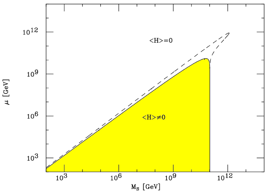
Figure 4: The critical line separating the broken and unbroken phases. Here $\mu$ is defined at the scale $M_{S}$ and we have fixed the top Yukawa coupling corresponding to $m_{t}=172.7$ GeV for large $\tan\beta$. Scalar universality and gaugino unification is assumed with boundary conditions at the GUT scale $m^{2}=M^{2}=M_{S}^{2}$, $A=0$ and $B=0$ (solid line), $B=\sqrt{2}M_{S}$ (dashed line).

The critical line in the $\mu$–$M_{S}$ plane, corresponding to eq. (25), is shown in fig. 4, in the case of scalar universality and gaugino unification with $m=M=M_{S}$, $A=0$ and $B=0$ (solid line), $B=\sqrt{2}M_{S}$ (dashed line) at the GUT scale. To understand the shape of these curves, let us indicate by $\bar{Q}_{c}$ the critical RG scale for $\mu=0$ and let us start with the case in which ${\tilde{m}}_{1}^{2}+{\tilde{m}}_{2}^{2}-|B|^{2}>0$ for $Q>\bar{Q}_{c}$ (as for the solid line of fig. 4). Then, in ordinary RG flows with $d{\tilde{m}}_{2}^{2}/d\ln Q>0$, an increase in $\mu$ will lower the value of $Q_{c}$. Let us study the critical line close to $M_{s}=\bar{Q}_{c}$. The small eigenvalue of ${\cal M}^{2}$ is

$$\lambda_{small}\simeq{\tilde{m}}_{2}^{2}+(1-r_{B})\mu^{2}+O(\mu^{4}),$$ (26)

where $r_{B}=|B|^{2}/{\tilde{m}}_{1}^{2}$. By using the qualitative behaviour $2{\tilde{m}}_{2}^{2}=\alpha M_{S}^{2}\ln M_{S}/\bar{Q}_{c}$, the critical curve is then given by

$$\lambda_{small}=0\quad\Rightarrow\quad\mu^{2}\simeq\frac{\alpha}{2(1-r_{B})}M_{S}^{2}\ln\bar{Q}_{c}/M_{S}\equiv f^{2}(M_{S}).$$ (27)

This equation implies that in the region $M_{S}\sim\bar{Q}_{c}$, which is favored when the number of vacua grows with $M_{S}$, there exist a moderate $O(\alpha)$ hierarchy also between $\mu^{2}$ and $M_{S}^{2}$. To see how this works explicitly, let us make the simple assumption on the distribution of vacua

$$dN\propto dM_{S}^{n}d\mu^{m}$$ (28)

with $m,n>0$. The Weak Principle restricts the acceptable vacua to lie in the region

$${\cal D}_{\mu}:~{}0<M_{S}<\bar{Q}_{c},~{}0<\mu<f(M_{S}).$$ (29)

Since $m_{Z}^{2}\simeq-2\lambda_{small}$, the average ratio $m_{Z}^{2}/M_{S}^{2}$ is given by

$$\left\langle\frac{m_{Z}^{2}}{M_{S}^{2}}\right\rangle\simeq\frac{\int_{{\cal D}_{\mu}}dN~{}\left[\alpha\ln\frac{Q_{c}}{M_{S}}-2(1-r_{B})\frac{\mu^{2}}{M_{S}^{2}}\right]}{\int_{{\cal D}_{\mu}}dN}=\frac{\alpha}{n+m}.$$ (30)

This shows that an independent scanning of $\mu$ changes eq. (10) simply by the replacement $n\to n+m$. The extra suppression is easy to understand, since a positive $m$ pushes $\mu$ towards the critical line, as a positive $n$ pushes $M_{S}$. The average ratio $\mu^{2}/M_{S}^{2}$ is instead

$$\left\langle\frac{\mu^{2}}{M_{S}^{2}}\right\rangle=\alpha~{}\frac{m}{4(1-r_{B})(n+m)}.$$ (31)

This shows that higgsinos are lighter than the typical supersymmetric particles by the square root of a loop factor.

Using $\sin 2\beta=2B\mu/(m_{1}^{2}+m_{2}^{2})$, we can express the average value of $\tan\beta$ as

$$\left\langle\tan\beta\right\rangle\simeq\frac{1}{\sqrt{r_{B}}}\left\langle\frac{M_{S}}{\mu}\right\rangle.$$ (32)

Therefore, $\tan\beta\sim 1/{\sqrt{\alpha}}\sim 5$–$10$ is the most natural expectation in this framework. This is welcome, because $|\cos 2\beta|\simeq 1$ plays a non-negligible role in pushing the mass of the lightest Higgs above the LEP bound. The generic prediction with soft parameters of the same order of magnitude is $\tan\beta=O(1)$, and it is well known that large $\tan\beta$ can be obtained only with a fine tuning of order $1/\tan\beta$ in $B\mu$. In our scenario, $\tan\beta\gg 1$ is just an added bonus of statistical criticality.

So far we have considered the case in which ${\tilde{m}}_{1}^{2}+{\tilde{m}}_{2}^{2}-|B|^{2}$ is always positive for $Q>\bar{Q}_{c}$. If this is not the case, the coefficient of $\mu^{2}$ in eq. (25) becomes negative before ${\tilde{m}}_{2}^{2}$, in the RG evolution starting from $M_{GUT}$. Therefore we expect that the most probable values of $\mu/M_{S}$ are of order unity, with no loop-factor suppression. This is confirmed by the result shown by the dashed line in fig. 4, which corresponds to the case of a large $B$.

In conclusion, the Weak Principle and statistical considerations based on an independent scan of $M_{S}$ and $\mu$ offer a solution to the $\mu$ problem, since the most probable values of $\mu$ turn out to be close to $M_{S}$. Moreover, in the case of positive ${\tilde{m}}_{1}^{2}+{\tilde{m}}_{2}^{2}-|B|^{2}$ for $Q>\bar{Q}_{c}$ (which is actually the most likely situation for typical soft terms of comparable sizes), our anthropic assumption gives the testable prediction that both $\mu/M_{S}$ and $1/\tan\beta$ are of the order of the square of a loop factor.

5 Dynamical Criticality

Our environmental argument to explain (if not post-dict) the little hierarchy of the minimal supersymmetric SM followed very closely Weinberg’s approach to the cosmological constant problem. Like for the cosmological constant, we think it is instructive to see why a dynamical mechanism, where $M_{S}$ is a dynamical rather than aleatory variable, is difficult to be realized.

It is well known that directions which are flat in the supersymmetric limit can dynamically generate 1-loop hierarchies via the Coleman-Weinberg mechanism. Indeed, in the presence of soft supersymmetry breaking, the effective potential along a flat direction $\phi$ can be written in general as $V=m^{2}(\phi)\phi^{2}$, where $m^{2}$ is a running effective mass squared. If, starting from a positive value at some high-energy scale, $m^{2}$ crosses zero at some smaller $\phi_{c}$, then $m^{2}(\phi)=\alpha M_{S}^{2}\ln\phi/\phi_{c}$ and the minimum of the potential will be at $\phi=\phi_{c}/\sqrt{e}$, where $e$ is Napier’s constant. At this minimum, $m^{2}$ is one-loop suppressed with respect to the typical soft mass scale thus dynamically realizing a little hierarchy. Barbieri and Strumia [14] have proposed a set up where a Coleman-Weinberg potential explains the little hierarchy. Following ref. [25] (see also ref. [26]), these authors have considered the situation in which the overall supersymmetric scale $M_{S}$ in eq. (3) is itself a scalar field, a modulus, with respect to which the potential should be minimized. The latter can generally be written as

$$V(M_{S},H_{1},H_{2})=V_{MSSM}(M_{S},H_{1},H_{2})+V_{S}(M_{S}),$$ (33)

where $V_{MSSM}$ represents the ordinary potential of the supersymmetric SM, with terms quadratic and quartic in the Higgs fields and with the running soft mass matrix ${\cal M}^{2}$. If, for some reason, $V_{S}$ could be neglected, then the minimization of $V_{MSSM}$ would dynamically realize an $O(\alpha)$ hierarchy between $\langle{H}\rangle^{2}$ and $M_{S}^{2}$. Indeed, under the same assumptions of sect. 3, $V_{MSSM}$ is strictly positive for $M_{S}>Q_{c}$. For $M_{S}<Q_{c}$ we can minimize $V_{MSSM}$ with respect to $H_{1,2}$ thus yelding an effective negative definite potential for $M_{S}$

$$V_{MSSM}^{\rm eff}(M_{S})=-\frac{2M_{S}^{4}}{g_{2}^{2}+g_{1}^{2}}~{}\frac{\left[c^{2}_{1}(M_{S})c^{2}_{2}(M_{S})-c_{3}^{4}(M_{S})\right]^{2}}{\left[c^{2}_{1}(M_{S})+c^{2}_{2}(M_{S})\right]^{2}-4c_{3}^{4}(M_{S})},$$ (34)

where, as before, the Higgs mass parameters are expressed as $m_{i}^{2}=c_{i}^{2}M_{S}^{2}$ $(i=1,2,3)$. Here to simplify the notation we have neglected the top-stop corrections to the Higgs quartic coupling. Expanding the $c_{i}$ in $\ln Q_{c}/M_{S}$, we find (indicating schematically the powers of loop factors for later use)

$$V_{MSSM}^{\rm eff}(M_{S})=-\frac{\alpha}{(4\pi)^{3}}M_{S}^{4}\ln^{2}\frac{Q_{c}}{M_{S}}\left[1+O\left(\frac{\alpha}{4\pi}\ln\frac{Q_{c}}{M_{S}}\right)\right],$$ (35)

which, at leading order in $\alpha$, is minimized at $\ln Q_{c}/M_{S}=1/2$. Compared to our eq. (10), this result correspond to dynamically predicting $n=2$ which, in principle, is a testable relation among soft parameters at the weak scale. It falls short, as already explained, to fully account for the little hierarchy, but nonetheless it is a remarkable result.

Unfortunately this result totally rests on our assumption of negligible $V_{S}(M_{S})$. Now, $V_{S}$ consists of two pieces: $V_{S}=V_{S}^{(1)}+V_{S}^{(2)}$. The first is truly incalculable, as it is quadratically divergent with the cut-off $V_{S}^{(1)}=\Lambda^{2}M_{S}^{2}$. There is no symmetry reason to really control this contribution, which for $\Lambda\sim M_{P}$ becomes, understandably, of the order of the supersymmetry breaking scale in the hidden sector $M_{I}^{4}$. The presence of $V_{S}^{(1)}$ does not only disrupt our dynamically critical minimum, but also implies a mimimum for $M_{S}$ which is either $0$ or $O(\Lambda)$. In other words $M_{S}$ is no longer a flat direction. Without any solid physical motivation one must then assume that by some clever short-distance conspiracy $V_{S}^{(1)}\equiv 0$. Yet this not sufficient, due to the second contribution

$$V_{S}^{(2)}=c_{0}(M_{S})M_{S}^{4}\left[1+O\left(\alpha(M_{S})\right)\right],$$ (36)

where the $O(\alpha)$ term indicates threshold correction effects at the supersymmetric scale and where $c_{0}$ satisfies an RG equation

$$\frac{dc_{0}}{d\ln Q}=\frac{1}{64\pi^{2}}\left[\frac{\rm StrM^{4}}{M_{S}^{4}}+O\left(\frac{\alpha}{4\pi}\right)\right].$$ (37)

Here $M$ is the mass matrix of all particles that become massive through their couplings to $M_{S}$ including, in particular, the supersymmetric partners of SM fields. The natural size of $c_{0}$ is $\sim 1/(4\pi)^{2}\ln M_{P}/M_{S}$, which makes $V_{S}^{(2)}$ parametrically bigger than $V_{MSSM}^{\rm eff}$ in the region $M_{S}\sim Q_{c}$. Then, in order to preserve the minimum of the full potential $V_{MSSM}^{\rm eff}+V_{S}^{(2)}$ near the critical point $M_{S}\sim Q_{c}$, also $V_{S}^{(2)}$ should independently have a minimum in this region. As the stationary points of $V_{S}^{(2)}$ are determined by dimensional transmutation through the logarithmic evolution of $c_{0}$, this coincidence represents a tuning, which we can roughly estimate to be of order $1/(\ln M_{P}/Q_{c})$. Unfortunately, this is precisely what a dynamical-relaxation model was designed to avoid. Moreover the presence of $V_{S}^{(2)}$ would destroy the prediction $\ln Q_{c}/M_{S}=\frac{1}{2}$. Finally one could argue that, although there is no solid field-theoretic reason to neglect $V_{S}$, perhaps this could follow from whatever mechanism solves the cosmological constant problem. We believe it is difficult to imagine how this could work. Indeed from a strict field-theoretic point of view the only distinction between $V_{MSSM}^{\rm eff}$ and $V_{S}^{(2)}$ is diagrammatic: the latter is determined by 1PI diagrams of supersymmetric SM fields, while the former involves also the one-particle reducible diagrams with tree-level Higgs exchange. How can the solution of the cosmological constant problem distinguish among different contributions to the potential of the same field $M_{S}$? Perhaps the only way to proceed is to see if there are consequences following from the vanishing of the potential at the minimum. Neglecting $V^{(1)}_{S}$, again without any explanation, the potential $V=c_{\rm eff}(M_{S})M_{S}^{4}$ consists of the addition of eq. (35) and eq. (36). The coefficient $c_{\rm eff}$ varies logarithmically with $M_{S}$, and it is in principle possible to fine tune the parameters so that $c_{\rm eff}$ and its derivative $c_{\rm eff}^{\prime}$ vanish simultaneously at some point. This point would correspond to a minimum with vanishing vacuum energy. It is easy to see that even this criterion in no way singles out the minimum of eq. (35).

6 Distribution of Supersymmetry-Breaking Scales

In this section we shall produce an argument on the possible distribution of the supersymmetry-breaking scale based on simple effective field theory. Our considerations and results are in line with what was previously found in type IIB Calabi-Yau orientifolds [21] or, in the same spirit of this section, in effective supergravity [27].

Suppose we have a general supersymmetric theory with $N$ chiral superfields $\Psi_{i}$, and a general superpotential $W(\Psi)$ and Kähler potential $K(\Psi,\Psi^{\dagger})$. We will assume that both of them include higher-dimension operators suppressed by some fundamental scale $M_{*}$, that we set to unity in this discussion. We will also ignore supergravity corrections by assuming that $M_{*}$ is parametrically smaller than $M_{P}$; all the vacua that we will find in our analysis below are then smoothly deformed into vacua of the full theory with supergravity effects included.

Of course, there will be a large number (exponential in $N$) of supersymmetric minima associated with the stationary points of $W$. However, we also expect to have a large number of metastable non-supersymmetric minima. It is easy to see that this is only possible due to higher-order terms in the Kähler potential. Indeed, with a canonical Kähler potential, any non-supersymmetric extremum is either a saddle point or it is associated with an exactly flat direction. Consider, for instance, the theory of a single chiral superfield with

$$W=a_{1}X+\frac{a_{3}}{3}X^{3}+\frac{a_{5}}{5}X^{5}+\cdots.$$ (38)

For simplicity, to begin with we assume a discrete $R$ symmetry that makes the superpotential odd in $X$ and makes $K$ a function only of $X^{\dagger}X$. For generic coefficients $a_{i}$, supersymmetric minima do exist. There is also a local maximum of the potential at $X=0$ with a quadratic instability along the direction where $a_{1}^{*}a_{3}X^{2}$ is real and negative. If we tune $a_{3,5,..}=0$, then we have supersymmetry breaking but also an exactly flat direction for $X$. This is why an arbitrarily small $a_{3,5..}$ can restore supersymmetry; it lifts the flat direction and drives the field to the supersymmetric minimum.

However, the story changes if we have corrections to the Kähler potential

$$K=X^{\dagger}X-\frac{c_{2}}{4}(X^{\dagger}X)^{2}+\frac{c_{4}}{9}(X^{\dagger}X)^{3}+\cdots,$$ (39)

because the higher-order terms in $K$ can also lift the flat direction and, if $c_{2}$ is large enough relative to $a_{3}$, stabilize a non-supersymmetric vacuum at $X=0$. Indeed, the potential is

$$V=\frac{|a_{1}+a_{3}X^{2}+a_{5}X^{4}+\cdots|^{2}}{1-c_{2}X^{\dagger}X+c_{4}(X^{\dagger}X)^{2}+\cdots}.$$ (40)

As long as

$$2|a_{3}|<|a_{1}|c_{2},$$ (41)

there is a non-supersymmetric local minimum at $X=0$. Note that the condition to find a non-supersymmetric local minimum does not depend on the values of $a_{5,...}$ and $c_{4,..}$; the reason is that these terms do not contribute to the quadratic curvature around the extremum at $X=0$.

Suppose we mediate the supersymmetry breaking to the SM sector via higher-dimensional operators, so that the overall scale of the soft terms is $M_{S}\sim|F_{X}|\sim|a_{1}|$ (working in units with $M_{*}=1$). For $c_{2}\sim O(1)$, to get a small $M_{S}$, we need not only $|a_{1}|\sim M_{S}$ but also $|a_{3}|\lower 3.01385pt\hbox{$\;\stackrel{{\scriptstyle\textstyle<}}{{\sim}}\;$}M_{S}$ to be small. If the $X$ sector coupled to a landscape of vacua, so that the complex parameters $a_{1},a_{3}$ scan, it is natural that, when they are small, they scan with a uniform distribution. So, since these are two complex parameters, the number of vacua with supersymmetry breaking scale smaller than $M_{S}$ is

$$N(M_{S})\propto M_{S}^{4}.$$ (42)

Let us now consider the most general case where $X$ is not charged under any symmetries, so that $W$ and $K$ are general functions of $X$. By shifting $X$, we can always assume without loss of generality that there is an extremum for $X$ located at $X=0$, and we can expand $W,K$ around this point

$$W=\sum_{n}\frac{a_{n}}{n}X^{n},\,\,~{}~{}~{}~{}K=\sum_{p,q}\frac{c_{pq}}{(p+1)(q+1)}X^{(p+1)}X^{\dagger(q+1)},$$ (43)

with $c_{00}=1$ and $c_{pq}^{*}=c_{qp}$. The potential, expanded at quadratic order in $X$, is

$$V=\frac{\left|\partial_{X}W\right|^{2}}{\partial_{X}\partial_{X^{\dagger}}K}=|a_{1}|^{2}+\left(k_{1}X+k_{2}X^{2}+{\rm h.c.}\right)+k_{3}|X|^{2}+\dots$$ (44)

$$k_{1} \equiv a_{1}^{*}\left(a_{2}-a_{1}c_{10}\right)$$ (45)

$$k_{2} \equiv a_{1}^{*}\left(a_{3}-a_{1}c_{20}\right)-c_{10}k_{1}$$ (46)

$$k_{3} \equiv |a_{2}|^{2}-|a_{1}|^{2}c_{11}-\left(c_{10}^{*}k_{1}+{\rm h.c.}\right).$$ (47)

The conditions to have a stable local minimum at $X=0$ with a supersymmetry-breaking scale equal to $M_{S}$ are

$$|a_{1}|=M_{S},~{}~{}~{}~{}~{}k_{1}=0,~{}~{}~{}~{}~{}|k_{3}|>2|k_{2}|.$$ (48)

For $c_{pq}=O(1)$, these conditions require that $|a_{1,2}|=O(M_{S})$ and $|a_{3}|\lower 3.01385pt\hbox{$\;\stackrel{{\scriptstyle\textstyle<}}{{\sim}}\;$}M_{S}$. If the 3 complex parameters $a_{1,2,3}$ scan uniformly, then we obtain

$$N(M_{S})\propto M_{S}^{6}.$$ (49)

Note though that we can get different powers with different assumptions about the landscape sector. For instance, if it has a CP symmetry that makes all the parameters real, then we would have $N(M_{S})\propto M_{S}^{3}$, while if it also has the discrete $R$ symmetry of the previous example we would have $N(M_{S})\propto M_{S}^{2}$.

Of course the non-supersymmetric minima we are considering are unstable to decaying to a supersymmetric vacuum, but the lifetime can be exponentially long. Indeed, we expect the bounce action to scale like $S\sim(\Delta X)^{4}/\Delta V$ where $\Delta X$ and $\Delta V$ are the shifts in field expectation value and potential energy between the two minima. In our case, $\Delta V=|a_{1}|^{2}$ and the location of the closest supersymmetric minimum is determined by the quartic term $a_{4}$ in $W$ and therefore $\Delta X\sim|a_{1}|^{1/3}$. This gives a lifetime $\Gamma\sim{\rm exp}-(M_{*}/M_{S})^{2/3}$, which is extremely small as soon as supersymmetry is broken below $M_{*}$.

We have phrased the discussion as though the $X$ sector is separate from the landscape sector, but in fact our conclusions apply to supersymmetry breaking on a generic supersymmetric landscape. It is clear that in order to find supersymmetry-breaking extrema, some fields in the theory must become light; indeed, there must be a massless goldstino. However with a completely generic superpotential, we expect that all the fields are heavy with $O(1)$ masses. In some places in field space, though, it may happen that one field $X$ is light while the remaining fields $\phi_{i}$ are heavy. We can then expand $W$ as

$$W=W_{0}(\phi)+W_{1}(\phi)X+\frac{1}{2}W_{2}(\phi)X^{2}+\frac{1}{3}W_{3}(\phi)X^{3}+\cdots$$ (50)

with the remaining fields $\phi$ having an exponentially large number of supersymmetric minima. In these minima, the parameters in the $X$ theory will scan, and again, when these parameters are small, the scanning can be taken to be flat.

Note that the scanning for the vacuum energy is completely independent of the supersymmetry breaking scale [28]. In all vacua (supersymmetric and non-supersymmetric), we will in general have $\langle W\rangle\equiv a_{0}\neq 0$. When gravity is turned on, this gives a negative contribution to the cosmological constant $\Lambda_{SUSY}=-3|W|^{2}/M_{P}^{2}$, which is parametrically unrelated to the scale of supersymmetry breaking. For a uniformly-distributed complex parameter $a_{0}$, the scanning measure is $d^{2}a_{0}=|W|d|W|=d\Lambda_{SUSY}$, i.e. there is uniform measure on cosmological-constant space. Therefore, the request of a small cosmological constant does not impose additional constraints on the statistical distribution of $M_{S}$.

As we have already mentioned there will also be an exponentially large number of supersymmetric stationary points, where all the landscape fields have generically $O(1)$ masses. What role can these vacua play in our argument? If these landscape vacua remain exactly supersymmetric even after including the possible infrared dynamics of some hidden gauge group, then they do not play any role in any selection criteria. Our universe does not appear to be supersymmetric. It is still possible, however, that at these minima some low-energy group with a supersymmetry-breaking infrared dynamics survives. It is natural to expect the distribution of $M_{S}$ from these vacua to be roughly logarithmic $dN\propto d\ln M_{S}$ [29], very much like the case of $\Lambda_{\rm QCD}$ considered in sect. 3. If the total number of vacua from this branch were large enough, then it would swamp the distribution of $M_{S}$ coming from the branch of local supersymmetry-breaking minima we focussed on so far. In that case, the total distribution of $M_{S}$ would be essentially $dN\propto d\ln M_{S}$, and the Weak Principle would predict $M_{S}\ll Q_{c}$. However the relative weight in vacuum statistics of this branch with dynamical supersymmetry breaking very strongly depends on microphysics inputs we do not control. On one side, it is not clear how generic it is that these hidden gauge groups lead to dynamical supersymmetry breaking. Also, there is no universal rationale to count the supersymmetric versus non-supersymmetric local minima, even with a simple landscape model with $N$ chiral fields $\phi_{i}$ ($i=1,...,N$). Assume, for instance, the superpotential is a generic polynomial of degree $M+1$ in $\phi_{i}$. Then the number of classically supersymmetric vacua determined by the equation

$$\partial_{i}W=0$$ (51)

scales like $M^{N}$. The non-supersymmetric stationary points are determined by the equation

$$\partial_{j}\bigl{(}\frac{\partial_{i}W}{\partial_{i}\partial^{k}K}\bigr{)}=0\,.$$ (52)

It is easy to see that, by suitably choosing the Kähler potential, there can be more solutions to eq. (52) than to eq. (51). For instance, take the case of just one superfield $X$ with superpotential and Kähler potential given by

$$W=\exp\left(-\lambda X\right),~{}~{}~{}~{}K=2X^{\dagger}X-{\rm Si}\left(X^{\dagger}X\right),$$ (53)

where $\lambda$ is a coupling constant and ${\rm Si}(x)$ is the sine-integral function, such that the Kähler metric is non-singular and positive definite. This gives a scalar potential

$$V=\frac{\lambda^{2}e^{-\lambda(X+X^{\dagger})}}{2-\cos(X^{\dagger}X)},$$ (54)

which can reach its supersymmetric vacuum only at $X\to\infty$, but has an infinite number of non-supersymmetric local minima. This result can be generalized to the case of $N$ fields. Therefore, depending on the properties of the Kähler potential, there may or there may not be more non-supersymmetric than supersymmetric vacua.

The results of this paper depend on the assumption that the tree-level supersymmetry-breaking vacua dominate in number over those with dynamical supersymmetry breaking. It is however remarkable that once this assumption is made the distribution of supersymmetry-breaking vacua depends on a few universal and basic ingredients. Our conclusion is that, for a “generic” theory with a large $N$ number of fields, there can be a huge number of non-supersymmetric vacua. In the neighborhood of any one of these vacua, the breaking of supersymmetry can be characterized by a single field $X$ getting an $F$-component, and $M_{S}$ has a distribution

$$N(M_{S})\propto M_{S}^{n},$$ (55)

where $n$ can run from $2$ to $6$ depending on assumptions on the structure of the landscape sector, with $n=6$ the most “generic”.

Note that for all $n>2$, we have a huge preference for high-scale supersymmetry breaking; in fact, the tuning it takes to get low-energy supersymmetry with $m_{Z}\sim M_{S}$ is much bigger than the standard hierarchy problem $\sim m_{Z}^{2}$. For $n=2$, it is about as tuned as the usual hierarchy problem, although if we manage to argue that $M_{S}$ is a loop factor bigger than $m_{Z}$, we win in tuning by a factor $(M_{S}/m_{Z})^{2}$. However, as we argued in this paper, if $Q_{c}$ has a maximum, then the statistical preference for high scale $M_{S}$ is eliminated by the anthropic prior that electroweak symmetry be broken (Weak Principle). The little hierarchy remains as the only detectable signal of an extremely atypical choice of vacuum, which is dictated by the anthropic prior.

The main result of our paper relies on the assumption of softly-broken supersymmetry. For instance if supersymmetry were broken at the cut-off scale, our minimal scenario, where only the overall value of $M_{S}$ scans, would hardly be tenable. In that case, all higher supercovariant derivative terms in the action would affect the Higgs potential and there could be plenty of other vacua where $\langle H\rangle$ is not controlled by radiative electroweak breaking. However, if we have such a preference for breaking supersymmetry at a high scale, what stops us from going all the way up to the fundamental scale $M_{*}$? The answer is metastability of the non-supersymmetric vacuum. As we said, one source of instability is given by tunneling of $X$ to the closest supersymmetric minimum with the parameters of its potential fixed. However, the local minimum for $X$ requires a special choice for the landscape fields $\phi$, in order to tune the parameters $a_{1,2,3}$ to small sizes. So another, potentially more important, source of vacuum decay is given by tunneling in $\phi$ space. It is reasonable to expect that the euclidean action for these processes will also be proportional to an inverse power of $M_{S}$. Thus, the total decay rate for the non-supersymmetric minimum is expected to be

$$\Gamma\sim M_{*}^{4}e^{-(M_{*}/M_{S})^{q}}$$ (56)

for some $q$. For large $M_{S}$, the decay rate is unsuppressed and therefore metastability (corresponding to $\Gamma<H_{0}^{4}$, where $H_{0}$ is the present value of the Hubble constant) puts a cutoff on the highest $M_{S}$

$$M_{S}^{max}\sim\frac{M_{*}}{\left[\ln(M_{*}/H_{0})\right]^{1/q}}.$$ (57)

This tells us that the only non-supersymmetric vacua that are cosmologically stable will indeed be approximately supersymmetric. In particular, this means that it is at least consistent to imagine that the only thing that scans is the overall scale of supersymmetry breaking. We do not have to worry about higher-derivative operators that would effectively make all the ratios of soft terms to scan, even with only a single source of supersymmetry breaking in $X$.

7 Phenomenological Consequences

The proximity of the critical scale $Q_{c}$ to the supersymmetric mass $M_{S}$ can be empirically tested at collider experiments. When the new-particle spectrum is known, one will be able to reconstruct the running of the Higgs mass parameters and observe if the critical condition for electroweak breaking is immediately achieved. However, even without a complete knowledge of the supersymmetric spectrum, we can obtain, under certain assumptions on the ratios of soft terms, some predictions on the Higgs and stop masses.

Let us work in the limit of large $\tan\beta$ (which is the most favourable case with respect to the Higgs mass bound), where the critical scale is determined by the condition $m_{2}^{2}(Q_{c})=0$. Since we expect a little hierarchy between the supersymmetric and the weak scale, in order to accurately compute the relevant physical quantities, we match to the one Higgs SM at the supersymmetric scale and take into account the leading RG evolution effects down to the weak scale. As it is convenient and customary, we choose the geometric average of the physical stop masses ($M_{\tilde{t}}^{2}=M_{{\tilde{t}}_{1}}M_{{\tilde{t}}_{2}}$) as the matching scale from which to compute the infrared logarithms. Notice that we do not need to specify a relation between $M_{S}$ and $M_{\tilde{t}}$ since, as discussed in sect. 3, $M_{S}$ appears in our equations only through the scheme-independent ratio $Q_{c}/M_{S}$.

After integrating out all supersymmetric particles and the additional neutral and charged Higgs bosons, the Higgs sector is described by the familiar SM scalar potential

$$V={m^{2}}|H|^{2}+\frac{\lambda}{2}|H|^{4}.$$ (58)

At the scale $M_{\tilde{t}}$, the Higgs parameters $m^{2}$ and $\lambda$ are determined by matching the supersymmetric theory with the SM:

$$m^{2}(M_{\tilde{t}})=m_{2}^{2}=-\left[\lambda_{t}^{2}\left(m_{\tilde{t}_{L}}^{2}+m_{\tilde{t}_{R}}^{2}+|A_{t}|^{2}\right)-\frac{g_{1}^{2}}{5}\left(M_{1}^{2}+\mu^{2}\right)-g_{2}^{2}\left(M_{2}^{2}+\mu^{2}\right)\right]\frac{3L_{S}}{8\pi^{2}}$$ (59)

$$\lambda(M_{\tilde{t}})=\left.\frac{g^{2}+g^{\prime 2}}{4}+\frac{3\lambda_{t}^{4}}{16\pi^{2}}X_{t}\right|_{M_{\tilde{t}}},$$ (60)

where $X_{t}$ is defined in the appendix and $L_{S}=\ln Q_{c}/M_{S}$. In eq. (60) we have also included a term which is formally a one-loop correction, but which can be numerically very important when the trilinear coupling $A_{t}$ is large. Consistently with our hypothesis, we can drop terms suppressed by inverse powers of $\tan\beta$ or proportional to $\mu$. Indeed, for natural values of the soft parameters of order $M_{S}$, the higgsino mass is expected to be of order $\mu={\cal O}(M_{S}/\tan\beta)$.

Next, we renormalize the parameters in eq. (58) to the scale of the top mass $m_{t}$, and also express the result in terms of the $\overline{\rm MS}$ top Yukawa $h_{t}$ computed at the top scale

$$m^{2}(m_{t}) = m^{2}(M_{\tilde{t}})K_{1}$$ (61)

$$\lambda(m_{t}) = \frac{g^{2}+g^{\prime 2}}{4}K_{2}$$ (62)

$$K_{1} \equiv 1-\frac{3h_{t}^{2}t_{S}}{8\pi^{2}}$$ (63)

$$K_{2} \equiv K_{1}^{2}(1+\delta)\simeq 1-\frac{3h_{t}^{2}t_{S}}{4\pi^{2}}+\delta$$ (64)

$$t_{S} \equiv \ln\frac{M_{\tilde{t}}}{m_{t}}.$$ (65)

Here $K_{1}$ is just the Higgs wavefunction renormalization due to top loops, while $\delta$ is the full RG improved top-stop additive correction to the Higgs quartic coupling, given in the appendix. We have used the SM RG evolution, including only effects from top-Yukawa and strong interactions. We kept linear terms in $t_{S}$ and $X_{t}$, and quadratic terms enhanced by $m_{t}^{2}/m_{Z}^{2}$.

The minimization of the potential in eq. (58) allows us to express the Higgs and the Z masses in terms of $m^{2}$ and $\lambda$: $m_{h}^{2}=-2m^{2}$ and $m_{Z}^{2}=-m^{2}(g^{2}+g^{\prime 2})/(2\lambda)$, where parameters are evaluated at the scale $m_{t}$. Using these equations, we can compute the Higgs mass and $M_{\tilde{t}}$ in terms of $m_{Z}$, $L_{S}$ and the ratios among soft terms:

$$m_{h}^{2} = K_{2}m_{Z}^{2}$$ (66)

$$M_{\tilde{t}}^{2} = \left|\frac{M_{\tilde{t}}^{2}}{m_{2}^{2}}\right|\frac{K_{2}}{2K_{1}}m_{Z}^{2}.$$ (67)

Here $M_{\tilde{t}}^{2}/m_{2}^{2}$, with $m_{2}^{2}$ given by eq. (59), obviously depends only on ratios of soft terms.

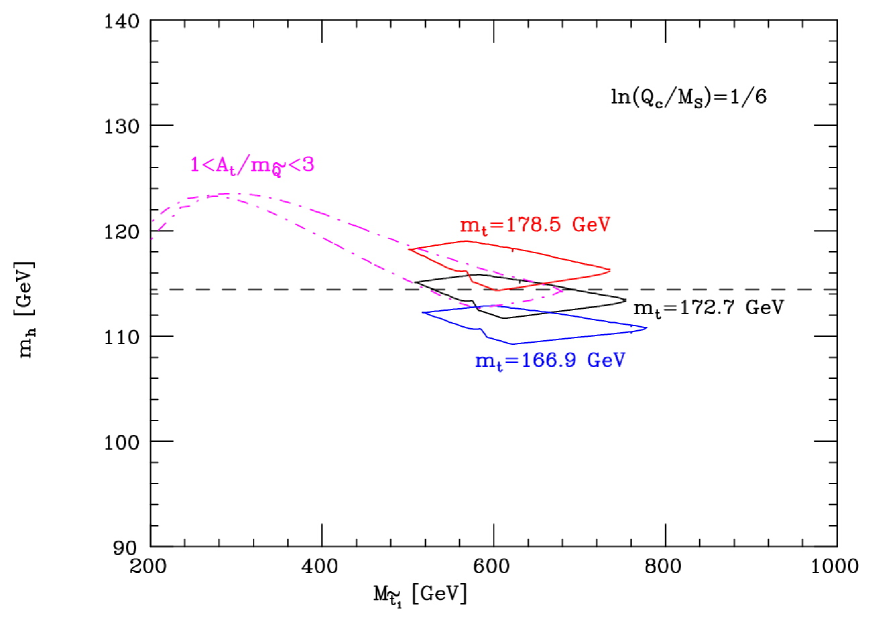
Figure 5: The solid lines are the boundaries of the regions of Higgs mass ($m_{h}$) and lightest stop mass ($M_{{\tilde{t}}_{1}}$) obtained by requiring $\ln Q_{c}/M_{S}=1/6$ and by scanning the ratios of soft parameters in the range $1/2<m^{2}_{\tilde{U}}/m^{2}_{\tilde{Q}}<2$, $0.8<A_{t}/m_{\tilde{Q}}<1$, $1/2<M_{3}^{2}/m^{2}_{\tilde{Q}}<2$, $1/10<M_{1,2}^{2}/m_{\tilde{Q}}^{2}<1$, under the constraint $M_{3}>200$ GeV, $M_{2}>100$ GeV, $M_{1}>50$ GeV, for the three values of $m_{t}$ indicated in the figure. The purple dot-dashed line is the boundary of the analogous region obtained for $1<A_{t}/m_{\tilde{Q}}<3$ and $m_{t}=172.7$ GeV. The dashed line is the present lower bound on a SM Higgs-boson mass $m_{h}>114.4$ GeV.

In fig. 5 we show the values of the Higgs mass $m_{h}$ and of the lightest stop mass $M_{{\tilde{t}}_{1}}$, obtained from eqs. (66)–(67) by fixing $L_{S}=1/6$ (which, as shown in sect. 6, is the most “generic” landscape prediction) and by varying the ratios of low-energy soft parameters in the range $1/2<m^{2}_{\tilde{U}}/m^{2}_{\tilde{Q}}<2$, $0.8<A_{t}/m_{\tilde{Q}}<1$, $1/2<M_{3}^{2}/m^{2}_{\tilde{Q}}<2$, $1/10<M_{1,2}^{2}/m_{\tilde{Q}}^{2}<1$. These ratios are varied independently, and therefore we are making no assumption of scalar universality or gaugino mass unification. The three regions shown in fig. 5 correspond to the top mass equal to its present central value $\pm 2\sigma$, and satisfy the requirement $M_{3}>200$ GeV, $M_{2}>100$ GeV, $M_{1}>50$ GeV. The restricted range of $A_{t}/m_{\tilde{Q}}$ is a natural consequence of the RG running of soft parameters up to a large scale. Indeed, the gluino mass gives a large renormalization correction to both parameters, focusing the low-energy value of this ratio, very much independently of the initial values of the various soft parameters at the high scale. For instance, taking the top Yukawa corresponding to large $\tan\beta$ and running up to the GUT scale, we find that $0.79(0.61)<A_{t}/m_{\tilde{Q}}<0.97(1.14)$ for any initial condition of universal scalar masses $m$, of unified gaugino masses $M$ and trilinear couplings $A$, such that $0<m^{2}/M^{2}<1(3)$ and $|A/M|<1(3)$.

The results in fig. 5 show how, for a small value of $\ln Q_{c}/M_{S}$, the Higgs mass is predicted to be very close to its experimental lower bound. On one hand, this can justify why searches for Higgs and supersymmetric particles have failed so far; on the other hand, it shows that Higgs and supersymmetric particles lie rather close to their experimental limits. With large values of $A_{t}$, heavier Higgs bosons and lighter stops can be obtained, as illustrated by the region in fig. 5 corresponding to a parameter scan in the range $1<A_{t}/m_{\tilde{Q}}<3$ (shown only in the case $m_{t}=172.7$ GeV). However, as shown above, such large values of this ratio are unnatural from the point of view of the high-energy theory. Very small values of $A_{t}/m_{\tilde{Q}}$ would further lower the prediction for $m_{h}$, but this also requires a tuning of soft-term boundary conditions at the high scale. The prediction on $m_{h}$ is rather sensitive on the precise value of $m_{t}$, as it is well known and as illustrated in fig. 5. A fixed value of $\ln Q_{c}/M_{S}$ also selects a limited range of stop masses. Of course, the precise values of the allowed $M_{{\tilde{t}}_{1}}$ depend on the choice of the interval in which the ratios of soft parameters are varied. The prediction shown in fig. 5 corresponds to the natural hypothesis that these ratios are not very different from unity.

8 Conclusions

Low-energy supersymmetry still remains the best known candidate to solve the hierarchy problem, although its natural prediction for new particles with masses around $m_{Z}$ has not been confirmed by LEP. The resulting necessity to push $M_{S}$, the scale of supersymmetric particle masses, almost an order of magnitude above $m_{Z}$ leads to an apparent fine tuning of few percent or worse. Although this is a much smaller problem than the original hierarchy, it is still worrisome for at least two reasons. First, the absence of fine tuning was, after all, the starting motivation for low-energy supersymmetry. Second, the necessary post-LEP mild tuning puts in question the chances of discovery at the LHC. Indeed the naturalness criterion, in spite of its intrinsic arbitrariness, is necessary to guarantee that supersymmetric particles are accessible to LHC energies, while the more quantitative requirement of a thermal relic density appropriate for dark matter is, by itself, not sufficient. Actually, taking into account LEP bounds and WMAP data, supersymmetric thermal dark matter requires rather uncharacteristic choices of parameters, raising the issue of a further source of tuning [30].

Different approaches have been proposed in the literature to reduce the amount of tuning or to explain a little hierarchy between $M_{S}$ and $m_{Z}$ [11, 12, 13, 14]. Large trilinear $A$ terms and a low scale for the original supersymmetry breaking alleviate the problem, but a complete solution may require a real modification of the minimal supersymmetric SM dynamics at the TeV. Here we have followed a drastically different approach, appealing to anthropic considerations to predict the most probable value of $M_{S}$, the scale of supersymmetric particle masses.

Symmetry principles have been so successful in particle physics that a general consensus has grown on the idea that nature is described by a final unique theory, completely determined by symmetry properties, possibly allowing no logically consistent modifications. More recently, this view has been challenged, as a result of both experimental observations and theoretical speculations. On one side, the evidence for dark energy reopened the question of the cosmological constant, which has a satisfactory anthropic justification [18], but no successful explanations based on symmetry or on dynamics. Also, the negative LEP searches for new physics have created some conflict in essentially all known models that can naturally explain the weak scale. On the theoretical side, the formulation of the string landscape [17] together with an inflationary picture has given a more solid justification for a multiverse description, where some of the properties of our universe are determined by environmental selection. If true, this description would represent the ultimate Copernican revolution, since neither the earth nor our observed universe have a central and unique role in nature.

From a scientific point of view, the great limitation of anthropic considerations, as opposed to speculations based on symmetry or dynamics, is the dearth of testable predictions. This is especially true when we cannot directly probe the properties of the statistical ensemble on which the anthropic principle is applied, as it is the case of the multiverse picture. Still, it is false that no physical consequences can be obtained. Predictions can be obtained, although they are different in nature from those derived by dynamics and can usually be expressed only in probabilistic terms. A celebrated example is the expectation that the cosmological constant is of the order of the critical density of our universe [18]. Another use of the anthropic principle is a change of perspective (as, e.g., in Split Supersymmetry [23]) where arguments based on symmetry properties (e.g. the hierarchy problem) are abandoned in favor of mere observational facts. In this paper we have offered a new example of an application of the anthropic principle to particle physics that can lead to testable predictions and we have derived, under certain assumptions, the most probable values of supersymmetric particle masses.

First of all, we have recast the hierarchy problem in terms of a criticality condition. Then, assuming a distribution of vacua where $M_{S}$ changes and imposing the anthropic request that electroweak symmetry must be broken by the Higgs field, we have obtained that $M_{S}$ is pushed close to $Q_{c}$, justifying with a statistical argument the quasi-criticality of low-energy supersymmetry. In this way we have derived a little hierarchy between $m_{Z}$ and $M_{S}$, a posteriori explaining why LEP has not discovered supersymmetry, while maintaining the prediction of discovery at the LHC. We have also discussed how our conclusions change as we modify the anthropic priors or the number of scanning parameters.

An interesting conclusion is found when the higgsino mass $\mu$ is allowed to scan independently of $M_{S}$. The anthropic argument shows that values of $\mu$ of the order of $M_{S}$ are preferred, giving a statistical (rather than dynamical) explanation for the approximate coincidence between the higgsino and gaugino masses. Actually, for moderate values of $B$, we predict that higgsinos are somewhat lighter and that $\tan\beta$ is moderately large. Once again, we recall that all predictions based on the anthropic principle refer to probability distributions. Indeed, we have found that, for the considered observables, the variance is of the order of the average ($\langle X^{2}\rangle\sim\langle X\rangle^{2}$ for an observable $X$) and therefore large statistical fluctuations are possible. In other words, our predictions suffer from a “cosmic variance” problem since, unfortunately, we can measure only the properties of a single universe, which is actually part of a large statistical ensemble.

Supersymmetry plays a crucial role in the mechanism we have presented, because it provides a dynamical explanation for the separation of scales between $Q_{c}$ and $M_{P}$. Here, like in ordinary low-energy supersymmetry, we take advantage of this natural hierarchy, but we are not trying to derive the absolute value of $M_{S}$. However, for a fixed value of the weak scale, we obtain a statistical distribution of the relative location of supersymmetry breaking, i.e. of $M_{S}/m_{Z}$, favoring a little hierarchy. Notice that in this respect, our mechanism could be applied to any theory with radiative electroweak breaking that predicts a separation between $Q_{c}$ and the fundamental high-energy scale. Our approach is less radical than Split Supersymmetry, where even the large hierarchy is attributed to anthropic considerations. However, while in Split Supersymmetry there is no justification for the proximity of the dark-matter particle mass to the weak scale, here we retain a dynamical explanation of this coincidence.

Our result essentially follows from the observation that electroweak breaking implies a maximum value of the supersymmetry-breaking scale, $M_{S}<Q_{c}$. On the other hand, the vacuum statistics prefer to break supersymmetry at the highest possible scale. Therefore, the combination of the two effects stabilizes $M_{S}$ very near the critical value. In other words, electroweak breaking is a rare phenomenon within the landscape and therefore, once we impose the prior $\langle{H}\rangle\neq 0$, the most likely situation is that $SU(2)\times U(1)$ is only barely broken, and supersymmetry has to live dangerously close to the critical line of unbroken symmetry.

We thank Nima Arkani-Hamed for collaboration throughout this project and for numerous suggestions. We also thank Savas Dimopoulos, Michael Douglas, and Andrea Romanino for discussions.

Appendix

Here we derive some of the equations for the Higgs parameters used in this paper. First consider the Higgs potential improved by the addition of the leading top-stop correction $\delta$ to the quartic coupling

$$V= m_{1}^{2}|H_{1}|^{2}+m_{2}^{2}|H_{2}|^{2}-m_{3}^{2}\left(H_{1}H_{2}+{\rm h.c.}\right)$$ (68)

$$+\frac{g^{2}}{8}\left(H_{1}^{\dagger}\vec{\sigma}H_{1}+H_{2}^{\dagger}\vec{\sigma}H_{2}\right)^{2}+\frac{g^{\prime 2}}{8}\left(|H_{1}|^{2}-|H_{2}|^{2}\right)^{2}+\frac{(g^{2}+g^{\prime 2})}{8}\delta|H_{2}|^{4},$$

$$\delta = \frac{3h_{t}^{4}}{(g^{2}+g^{\prime 2})\pi^{2}\sin^{4}\beta}\left[t_{S}+\frac{X_{t}}{4}+\frac{t_{S}}{32\pi^{2}}\left(3h_{t}^{2}-16g_{s}^{2}\right)\left(X_{t}+2t_{S}\right)\right]$$ (69)

$$X_{t} \equiv \frac{2\left(A_{t}-\mu/\tan\beta\right)^{2}}{M_{\tilde{t}}^{2}}\left[1-\frac{\left(A_{t}-\mu/\tan\beta\right)^{2}}{12M_{\tilde{t}}^{2}}\right],~{}~{}~{}~{}~{}~{}~{}~{}M_{\tilde{t}}^{2}\equiv M_{{\tilde{t}}_{1}}M_{{\tilde{t}}_{2}}$$ (70)

$$t_{S} \equiv \ln\frac{M_{\tilde{t}}}{m_{t}}.$$ (71)

Here $h_{t}$ is the $\overline{\rm MS}$ top Yukawa at $Q=m_{t}$ in the SM effective theory.

In the presence of a hierarchy between $m_{Z}$ and the pseudoscalar Higgs mass $m_{A}$, the eigenvalues of the mass matrix ${\cal M}^{2}$ defined by eq. (68) are

$$m^{2}_{lar} = (m_{1}^{2}+m_{2}^{2})\left[1+O\left(\epsilon_{Z}\right)\right]$$ (72)

$$m^{2}_{sma} = \frac{m_{1}^{2}m_{2}^{2}-m_{3}^{4}}{m_{1}^{2}+m_{2}^{2}}\left[1+O\left(\epsilon_{Z}\right)\right],$$ (73)

where $\epsilon_{Z}\equiv{m^{2}_{sma}}/{m_{lar}^{2}}\sim{m^{2}_{Z}}/{m_{A}^{2}}$ will be our expansion parameter. It is convenient to diagonalize ${\cal M}^{2}$ by redefining

$$\left(\begin{array}[]{c}H_{1}\\ H_{2}\end{array}\right)=\left(\begin{array}[]{cc}\cos\beta^{\prime}&-\sin\beta^{\prime}\\ \sin\beta^{\prime}&\cos\beta^{\prime}\end{array}\right)\left(\begin{array}[]{c}H\\ H^{\prime}\end{array}\right).$$ (74)

By integrating out $H^{\prime}$ in eq. (68) we find the effective potential for $H$

$$V_{eff}=\frac{m_{1}^{2}m_{2}^{2}-m_{3}^{4}}{m_{1}^{2}+m_{2}^{2}}|H|^{2}+\frac{g^{2}+g^{\prime 2}}{8}\left(\cos^{2}2\beta+\delta\sin^{4}\beta\right)|H|^{4}+O(\epsilon_{Z})$$ (75)

where, given that $\langle H^{\prime}\rangle/\langle H\rangle=O(\epsilon_{Z})$, the leading result simply amounts to setting $H^{\prime}=0$. Notice also that $\tan\beta\equiv\langle{H_{2}}\rangle/\langle{H_{1}}\rangle$ is equal to $\tan\beta^{\prime}$ at leading order in $\epsilon_{Z}$. By minimizing eq. (75) and expanding ${\cal M}^{2}$ around its zero at leading order in $L_{S}$ one obtains eq. (7).

We will now instead study the Higgs spectrum for arbitrary $m_{A}$, but, again, including the leading top-stop correction. This corresponds to finding the mass eigenvalues and mixing angles from the Higgs potential in eq. (68). Defining

$$\Delta=m_{Z}^{2}\sin^{2}\beta\,\delta\qquad\qquad\hat{m}^{2}_{2}=m_{2}^{2}+\frac{\Delta}{2},$$ (76)

the result is

$$m_{Z}^{2} = \frac{2\left(m_{1}^{2}-\hat{m}_{2}^{2}\tan^{2}\beta\right)}{\tan^{2}\beta-1}\qquad\qquad\sin 2\beta=\frac{2m_{3}^{2}}{m_{A}^{2}}$$ (77)

$$m_{A}^{2} = m_{1}^{2}+\hat{m}_{2}^{2}\qquad\qquad m_{H^{+}}=m_{A}^{2}+m_{W}^{2}$$ (78)

$$m_{h,H}^{2} = \frac{1}{2}\left\{m_{A}^{2}+m_{Z}^{2}+\Delta\pm\sqrt{\left[\cos 2\beta(m_{A}^{2}-m_{Z}^{2})+\Delta\right]^{2}+\sin^{2}2\beta(m_{A}^{2}+m_{Z}^{2})^{2}}\right\}.$$ (79)

In the limit $m_{A}^{2}\to\infty$ the lightest Higgs mass becomes

$$m_{h}^{2}=m_{Z}^{2}(\cos^{2}2\beta+\delta\sin^{4}\beta),$$ (80)

in agreement with eq. (75). Notice that only the CP-even Higgs masses are formally affected by the presence of $\Delta$. The tree level relation $m_{h}^{2}<{\rm min}(m_{A}^{2},m_{Z}^{2})$ now becomes

$$m_{h}^{2}<{\rm min}(m_{A}^{2},m_{Z}^{2}+\Delta)\qquad {\rm for}\qquad m_{A}^{2}>m_{Z}^{2}\frac{\delta}{4+\delta}$$ (81)

$$m_{A}^{2}<m_{h}^{2}<m_{Z}^{2}+\Delta\qquad {\rm for}\qquad m_{A}^{2}<m_{Z}^{2}\frac{\delta}{4+\delta}.$$ (82)

Finally, the square of the $ZZh$ coupling $\lambda_{ZZh}^{2}$ is suppressed with respect to the SM value by a factor

$$\sin^{2}(\beta-\alpha)=\frac{1}{2}\left[1+\frac{m_{A}^{2}-m_{Z}^{2}\cos 4\beta+\Delta\cos 2\beta}{m_{H}^{2}-m_{h}^{2}}\right],$$ (83)

while the $ZZH$ and $ZAh$ couplings are proportional to $\cos(\beta-\alpha)$ like in the minimal supersymmetric SM. As can be seen from the above equations, in order to have a significant reduction in $\sin^{2}(\beta-\alpha)$ one needs $m_{A}^{2}<m_{Z}^{2}+\Delta$ as well as $\tan\beta\gg 1$. However in this region the $ZAh$ coupling is sizeable and moreover, for small $\Delta$, the threshold for $Ah$ production would be significantly below the maximal LEP2 energy. The experimental bound from $Ah$ production then requires a non-negligible $\Delta$ for this region to be viable. This is the reason why the allowed area in fig. 3 does not extend far away from the critical line: a sizeable top-stop contribution to $\Delta$ is needed.

References

- [1] E. Witten, Nucl. Phys. B 188 (1981) 513.
- [2] L. E. Ibanez and G. G. Ross, Phys. Lett. B 110 (1982) 215; L. Alvarez-Gaume, J. Polchinski and M. B. Wise, Nucl. Phys. B 221 (1983) 495.
- [3] R. Barbieri and G. F. Giudice, Nucl. Phys. B 306 (1988) 63; G. W. Anderson and D. J. Castano, Phys. Lett. B 347 (1995) 300 [arXiv:hep-ph/9409419].
- [4] Y. Okada, M. Yamaguchi and T. Yanagida, Prog. Theor. Phys. 85 (1991) 1; J. R. Ellis, G. Ridolfi and F. Zwirner, Phys. Lett. B 257 (1991) 83.
- [5] J. L. Feng, K. T. Matchev and T. Moroi, Phys. Rev. D 61 (2000) 075005 [arXiv:hep-ph/9909334].
- [6] G. F. Giudice and A. Masiero, Phys. Lett. B 206 (1988) 480.
- [7] LEP SUSY Working Group, mote LEPSUSYWG/01-03 (2001).
- [8] LEP Higgs Working Group, note LHWG/05-01 (2005).
- [9] B. de Carlos and J. A. Casas, Phys. Lett. B 309 (1993) 320 [arXiv:hep-ph/9303291]; S. Dimopoulos and G. F. Giudice, Phys. Lett. B 357 (1995) 573 [arXiv:hep-ph/9507282]; L. Giusti, A. Romanino and A. Strumia, Nucl. Phys. B 550 (1999) 3 [arXiv:hep-ph/9811386]; J. A. Casas, J. R. Espinosa and I. Hidalgo, JHEP 0411 (2004) 057 [arXiv:hep-ph/0410298].
- [10] R. Barate et al. [LEP Higgs Working Group], Phys. Lett. B 565 (2003) 61 [arXiv:hep-ex/0306033].
- [11] Z. Berezhiani, P. H. Chankowski, A. Falkowski and S. Pokorski, Phys. Rev. Lett. 96 (2006) 031801 [arXiv:hep-ph/0509311]; T. Roy and M. Schmaltz, JHEP 0601 (2006) 149 [arXiv:hep-ph/0509357]; C. Csaki, G. Marandella, Y. Shirman and A. Strumia, Phys. Rev. D 73 (2006) 035006 [arXiv:hep-ph/0510294].
- [12] P. Batra, A. Delgado, D. E. Kaplan and T. M. P. Tait, JHEP 0402 (2004) 043 [arXiv:hep-ph/0309149]. J. A. Casas, J. R. Espinosa and I. Hidalgo, JHEP 0401 (2004) 008 [arXiv:hep-ph/0310137].
- [13] K. Choi, A. Falkowski, H. P. Nilles and M. Olechowski, Nucl. Phys. B 718 (2005) 113 [arXiv:hep-th/0503216]; K. Choi, K. S. Jeong, T. Kobayashi and K. i. Okumura, Phys. Lett. B 633 (2006) 355 [arXiv:hep-ph/0508029]; R. Kitano and Y. Nomura, Phys. Lett. B 631 (2005) 58 [arXiv:hep-ph/0509039].
- [14] R. Barbieri and A. Strumia, Phys. Lett. B 490 (2000) 247 [arXiv:hep-ph/0005203].
- [15] P. C. Schuster and N. Toro, arXiv:hep-ph/0512189.
- [16] A. Pierce and J. Thaler, arXiv:hep-ph/0604192.
- [17] R. Bousso and J. Polchinski, JHEP 0006 (2000) 006 [arXiv:hep-th/0004134]; S. B. Giddings, S. Kachru and J. Polchinski, Phys. Rev. D 66 (2002) 106006 [arXiv:hep-th/0105097]; A. Maloney, E. Silverstein and A. Strominger, arXiv:hep-th/0205316; S. Kachru, R. Kallosh, A. Linde and S. P. Trivedi, Phys. Rev. D 68 (2003) 046005 [arXiv:hep-th/0301240]; L. Susskind, arXiv:hep-th/0302219.
- [18] S. Weinberg, Phys. Rev. Lett. 59 (1987) 2607; A. Vilenkin, Phys. Rev. Lett. 74 (1995) 846 [arXiv:gr-qc/9406010].
- [19] V. Agrawal, S. M. Barr, J. F. Donoghue and D. Seckel, Phys. Rev. D 57 (1998) 5480 [arXiv:hep-ph/9707380]; T. E. Jeltema and M. Sher, Phys. Rev. D 61 (2000) 017301 [arXiv:hep-ph/9905494]; H. Oberhummer, A. Csoto and H. Schlattl, Nucl. Phys. A 689 (2001) 269 [arXiv:nucl-th/0009046]; C. J. Hogan, arXiv:astro-ph/0602104.
- [20] N. Arkani-Hamed, S. Dimopoulos and S. Kachru, arXiv:hep-th/0501082.
- [21] S. Ashok and M. R. Douglas, JHEP 0401 (2004) 060 [arXiv:hep-th/0307049]; F. Denef and M. R. Douglas, JHEP 0405 (2004) 072 [arXiv:hep-th/0404116].
- [22] R. Harnik, G. D. Kribs and G. Perez, arXiv:hep-ph/0604027.
- [23] N. Arkani-Hamed and S. Dimopoulos, JHEP 0506 (2005) 073 [arXiv:hep-th/0405159]; G. F. Giudice and A. Romanino, Nucl. Phys. B 699 (2004) 65 [Erratum-ibid. B 706 (2005) 65] [arXiv:hep-ph/0406088]. N. Arkani-Hamed, S. Dimopoulos, G. F. Giudice and A. Romanino, Nucl. Phys. B 709 (2005) 3 [arXiv:hep-ph/0409232].
- [24] J. L. Feng, A. Rajaraman and B. T. Smith, arXiv:hep-ph/0512172; R. Dermisek and H. D. Kim, arXiv:hep-ph/0601036.
- [25] E. Cremmer, S. Ferrara, C. Kounnas and D. V. Nanopoulos, Phys. Lett. B 133 (1983) 61; J. R. Ellis, A. B. Lahanas, D. V. Nanopoulos and K. Tamvakis, Phys. Lett. B 134 (1984) 429.
- [26] C. Kounnas, F. Zwirner and I. Pavel, Phys. Lett. B 335 (1994) 403.
- [27] M. Dine, D. O’Neil and Z. Sun, JHEP 0507 (2005) 014 [arXiv:hep-th/0501214].
- [28] L. Susskind, arXiv:hep-th/0405189; M. R. Douglas, arXiv:hep-th/0405279.
- [29] M. Dine, E. Gorbatov and S. D. Thomas, arXiv:hep-th/0407043.
- [30] N. Arkani-Hamed, A. Delgado and G. F. Giudice, Nucl. Phys. B 741 (2006) 108 [arXiv:hep-ph/0601041].