Discovery of supersymmetry with degenerated mass spectrum

Abstract

Discovery of supersymmetric (SUSY) particles at the Large Hadron Collider (LHC) has been studied for the models where squarks and gluino are much heavier than the lightest supersymetric particle (LSP). In this paper, we investigate the SUSY discovery in the models with degenerated mass spectrum up to $m_{\rm LSP}\mathop{}_{\textstyle\sim}^{\textstyle<}0.7m_{\tilde{q}}$. Such mass spectrum is predicted in certain parameter region of the mixed modulas anomaly mediation (MMAM) model. We find that the effective transverse mass of the signal for the degenerated parameters shows the distribution similar to that of the background. Experimental sensitivity of the SUSY particles at the LHC therefore depends on the uncertainty of the background in this class of model. We also find that SUSY signal shows an interesting correlation between $M_{\rm eff}$ and ${\not\!\!E}_{\rm T}$ which may be used to determine the signal region properly to enhance the S/N ratio even if the sparticle masses are rather degenerated. The structure is universal for the models with new heavy colored particles decaying into visible particles and a stable neutral particle, dark matter.

I Introduction: Transverse Physics and its non-transverse limit

Minimal supersymmetric standard model (MSSM) is one of the most promising candidates of the physics beyond the standard model (SM) that may solve the hierarchy problem in the Higgs sector MSSM . The model predicts a set of superpartners (sparticles) whose charges are exactly the same to that of the SM partners but the spins are different by one half.

These sparticles will be directly searched at the Large Hadron Collider (LHC) at CERN, which is a $pp$ collider with 14 TeV center of mass energy. The LHC is scheduled to start in 2007. One of the interesting features of the MSSM model is the conserved R parity, and all sparticles are assigned to have odd R parity. Because of the conservation law, the lightest supersymmetric particle (LSP) is stable, and is assumed as a good candidate for the dark matter. At collider experiments, sparticles are produced in pairs, and a sparticle decay should produce at least one LSP. SUSY events at collider experiments therefore have a distinctive missing transverse momentum.

If supersymmetry (SUSY) is an exact symmetry, a particle and its superpartner have a same mass. Therefore SUSY must be broken spontaneously. The SUSY is considered to be broken in “hidden sector”, and the SUSY breaking will be mediated to our sector by mediation fields. The mechanism is already under severe constraints. For example, the mass of the sfermions with same charge must be universal so that they do not cause dangerous FCNC, or sfermion masses must be so heavy that correction from the SUSY sector is suppressed. This suggests that yet unknown symmetry/dynamics exists in the sector. The origin of the supersymmetry breaking and mediation mechanism may be understood indirectly by measuring masses of the SUSY particles. Therefore both the discovery and mass determination of the SUSY particle have been studied intensively in recent years TDR ; HP ; LHCLC .

If SUSY is broken at some high energy scale and the boundary conditions are universal at the scale, strongly interacting (SI) SUSY particles are heavier than electroweakly interacting (EWI) SUSY particles. For example, gaugino masses follow the relation

$$M_{1}:M_{2}:M_{3}\sim 0.4:0.8:2.4$$ (1)

in the minimal supergravity model, therefore the gluino is six times heavier than the bino-like particles. At the LHC, SI SUSY particles will be copiously produced in $pp$ collisions, and subsequently decay into lighter EWI SUSY particles.

The gluino and squark decays are associated with jets with high transverse momentum ($p_{T}$). The transverse momentum is the order of the gluino and squark masses. Moreover, because the LSP is significantly lighter than the gluino, the LSP from the gluino decay also has a high $p_{T}$. They would give a large missing transverse momentum to the SUSY events. In addition, decays of the EWI sparticles may produce high $p_{T}$ leptons. Events from the standard model (SM) processes do not have such high $p_{T}$ particles.

Motivated by these observations, following cuts are often applied to reduce the SM background events to the SUSY signal events TDR ;

• An event is required to have at least one jet with $p_{T}>100$ GeV and three jets with $p_{T}>50$ GeV within $|\eta|<3$,

• The effective mass of the event must satisfy $M_{\rm eff}>400$ GeV, where the effective mass is defined using the transverse missing energy (${\not\!\!E}_{\rm T}$) and the transverse momentum of four leading jets as:

  $$M_{\rm eff}\equiv\sum_{i=1,...4}p_{Ti}+{\not\!\!E}_{\rm T}.$$ (2)

  If the event has hard isolated leptons, the effective mass may be defined as follows:

  $$M_{\rm eff}\equiv\sum_{i=1,...4}p_{Ti}+\sum_{\rm leptons}p_{Tl}+{\not\!\!E}_{\rm T},$$ (3)

  where sum of the lepton $p_{T}$ can be taken over the leptons with $p_{T}>20$ GeV and $|\eta|<2.5$ GeV.

• The missing transverse energy must satisfy the relation:

  $${\not\!\!E}_{\rm T}>{\rm max}(0.2M_{\rm eff},100{\rm GeV}).$$ (4)

• The transverse sphericity $S_{T}$ must be greater than 0.2, where $S_{T}$ is defined as $2\lambda_{2}/(\lambda_{1}+\lambda_{2})$, with $\lambda_{1}$ and $\lambda_{2}$ being the eigenvalues of the $2\times 2$ sphericity tensor $S_{ij}=p_{ki}p_{kj}$ formed by summing over the transverse momentum of all calorimeter cells.

To reduce the background further, hard, isolated lepton(s) may be required. These cuts are good enough to reduce the SM backgrounds from $t\bar{t}$+$n$-jets and $W(Z)$+$n$-jets productions down to a manageable level, although the production cross section of the SM processes may be ${\cal O}(10^{4})$ higher than signal cross sections. While the SUSY production section reduces very quickly as sparticle masses increase beyond 1 TeV, but the signature peaks at higher $M_{\rm eff}$ where backgrounds can be ignored . Previous studies show that the squark and gluino with mass around 2.5 TeV can be found at the LHC in the minimal super gravity model (MSUGRA).

In MSUGRA, the SM background after the cuts can be neglected safely. Then, the distribution of accepted events are also useful to determine the mass scale of SUSY particles. For example, the peak of the $M_{\rm eff}$ distribution is sensitive to the squark and gluino masses. For the events with same flavor opposite sign dileptons, the invariant mass distributions, $m_{ll}$, $m_{jl}$, and $m_{jll}$, are useful to reconstruct the SUSY particle masses $m_{\tilde{\chi}^{0}_{1}}$, $m_{\tilde{\chi}^{0}_{2}}$, $m_{\tilde{q}^{0}_{1}}$ and $m_{\tilde{l}^{0}_{1}}$.

Recently it is pointed out that a string inspired model based on the flux compactification (KKLT models) LINDE predicts a mass relation different from that of the MSUGRA CHOI ; FLM ; YAMA . This is called mixed modulus anomaly mediation (MMAM) model. This model has a volume modulas $T$ and a compensator field of minimum supergravity model $C$ as a messenger of the SUSY breaking. The SUSY mass spectrum depends on the ratio of the two SUSY breaking parameters $F_{T}$ and $F_{C}$. The unification scale of the sparticle masses depends on the ratio. It is interesting that the unification scale of the soft SUSY parameters can be much lower than the GUT scale in this model. They may unify even at the weak scale for a special choice of the model parameters.

When sparticle masses are degenerated at the weak scale, we expect a reduced probability to have high $p_{T}$ jets, and smaller $M_{\rm eff}$ and ${\not\!\!E}_{\rm T}$ for given squark and gluino masses. This means that the standard SUSY cuts reduce the signal events as well, and SUSY discovery is more affected by the SM background.

Quantitative understanding of the SM background may be required in this case. Existing background estimates have large theoretical uncertainty coming from the scale of the strong coupling. Recently, several groups has emphasized importance to include the matrix element correction MANGANO ; RAINWATER ; TEV4LHC in the previous parton shower estimate of the background, which significantly change the background distribution in the signal region. When overlap between the signal and background distribution is large, as it is expected in the degenerated SUSY spectrum, the uncertainty of the background must be taken seriously, and we also need to reconsider the cuts to reduce the background.

The purpose of this paper is to illustrate the phenomenology of the degenerated supersymmetry. We take the MMAM model as an example. By changing the ratio $F_{C}/F_{T}$, the mass spectrum changes smoothly from MSUGRA-like one to anomaly-mediation-like one. In between, there are regions of parameters where squark, slepton, and gaugino masses are significantly degenerated compared with those expected in MSUGRA. The model therefore provides one dimensional parametrization from the “transverse signature” to its non-transverse limit. The investigation of our analysis may easily be extended to other SUSY/non-SUSY scenarios with ${\not\!\!E}_{\rm T}$ signature, such as the universal extra dimension model or little Higgs model with $T$ parity.

This paper is organized as follows. In section 2 we describe the MMAM model and its mass spectrum with an emphasis on the region of parameter space where sparticle masses are degenerated. In section 3, we describe our Monte Carlo simulations. In section 4, we study how SUSY event distribution depends on sparticle mass degeneracy and compare it with the background. We find that the signal $M_{\rm eff}$ distribution is quite similar to that of the background if $m_{\tilde{\chi}^{0}_{1}}\mathop{}_{\textstyle\sim}^{\textstyle>}0.5m_{\tilde{q},\tilde{g}}$. However we find a certain relation among ${\not\!\!E}_{\rm T}$ and $M_{\rm eff}$ that is universal for the model with heavy colored particle that decays into the stable neutral particle LHC will miss the SUSY signature if $m_{\tilde{\chi}^{0}_{1}}\mathop{}_{\textstyle\sim}^{\textstyle>}0.7m_{\tilde{q},\tilde{g}}$. Section 5 is devoted to discussions and conclusions.

II The MMAM model

II.1 Boundary conditions at GUT scale

In this section, we briefly describe the MMAM model following the notation in CHOI . In this model, all shape modulus and dilaton will be fixed by non-zero flux on a CY manifold in the Type IIB string theory. The low energy $N=1$ Lagrangian of this model is given by unfixed volume modulus $T$, compensator field $C$, and gauge and matter fields $W^{a}$ and $Q_{i}$ as

$$S_{N=1} = \int d^{4}x\sqrt{g^{C}}\left[d^{4}\theta CC^{*}(-3\exp(-K_{\rm eff}/3))\right.$$ (6)

$$\left.+\left\{\int d^{2}\theta\left(f_{a}W^{a\alpha}W^{a}_{\alpha}+C^{3}W_{\rm eff}\right)+h.c.\right\}\right].$$

Here $K_{\rm eff}=-3\ln(T+T^{*})+Z_{i}(T+T^{*})Q_{i}^{*}Q_{i}$, $g^{c}_{\mu\nu}$ is the 4D metric in the super conformal frame. $T=T_{0}+F_{T}\theta^{2}$ and $C=C_{0}+F_{C}\theta^{2}$ are the volume modulas and the chiral compensator superfield of $N=1$ SUGRA, respectively. $W_{\rm eff}=W_{0}(T)+\frac{1}{6}\lambda_{ijk}Q_{i}Q_{j}Q_{k}$ is the superpotential for $T$ and matter. $T$ dependent function $Z_{i}$ and $f_{i}$ may be expressed as

$$Z_{i}=\frac{1}{(T+T^{*})^{n_{i}}},\ \ f_{a}=T^{l_{a}},$$ (7)

where $n_{i}$ is the modular weights and $n_{i}=0(1)$ for matter fields located on D7 (D3) branes, and $n=1/2$ for matter living at brane intersections CHOI .

In KKLT model, $W_{0}=w_{0}-A\exp^{-aT}$, where the last term of $W_{0}$ expresses the non-perturbative effect such as the gaugino condensation in D7 brane, which fix the volume modulus, $w_{0}$ is the contribution of the flux. In addition to the $N=1$ supersymmetric action, there are contributions from anti-D3 branes which break supersymmetry and uplift the potential from AdS vacuum to (nearly Minkowski) de Sitter vacuum. The term is expressed by a spurion operator depending on $T$ and $C$, and minimum of the potential will be obtained by solving the effective $N=1$ action and the lifting potential.

The resulting theory is parametrized by $F_{C}/C_{0}\sim m_{3/2}$ and $F_{T}/(T+T^{*})$ . The SUSY breaking terms are obtained by expanding the action by $F_{T}$ and $F_{C}$. Here we define the soft terms as

$$L_{soft}=-\frac{1}{2}M_{a}\lambda^{a}\lambda^{a}-m_{i}^{2}|\tilde{Q}_{i}|^{2}-A_{ijk}y_{ijk}\tilde{Q}_{i}\tilde{Q}_{j}\tilde{Q}_{k}+hc$$ (8)

where $y_{ijk}$ is a canonically normalized Yukawa coupling

$$L_{\rm soft}=\frac{\lambda_{ijk}}{\sqrt{e^{-K_{0}}Z_{i}Z_{j}Z_{k}}}.$$ (9)

They are explicitly written as functions of $m_{3/2}$ and $R\equiv m_{3/2}(T+T^{*})/F_{T}$ as follows;

$$M_{a} = \left(\frac{l_{a}}{R}+\frac{b_{a}g^{2}_{GUT}}{16\pi^{2}}\right)m_{3/2}$$ (10)

$$m_{i}^{2} = \left(\frac{m_{i}}{R^{2}}+\frac{1}{R}\frac{\partial\gamma_{i}}{\partial\ln T}-\frac{1}{4}\frac{\partial\gamma_{i}}{\partial\ln\mu}\right)m_{3/2}^{2}$$ (11)

$$A_{ijk} = \left(\frac{1}{R}(m_{i}+m_{j}+m_{k})-\frac{1}{2}(\gamma_{i}+\gamma_{j}+\gamma_{k})\right)m_{3/2}$$ (12)

where $m_{i}=1-n_{i}$ and

$$\gamma_{r}=\mu\frac{d\ln Z_{r}}{d\mu}=\frac{1}{8\pi^{2}}\left(2\sum_{a}C^{a}_{r}g_{a}^{2}-d_{r}y^{2}\right)$$ (13)

with $C_{r}=\sum_{a}T_{a}^{2}(r)$, namely for matter in the fundamental representation $C^{3}_{F}=4/3$, $C^{2}_{F}=3/4$, $C^{\prime}=Y^{2}$. We only include the effect of the top Yukawa coupling $y$, therefore $d_{Q_{3}}=1$, $d_{T}=2$, $d_{H2}=3$ and $d_{i}=0$ otherwise.

The scale dependence of $\gamma_{i}$ is expressed as

$$\frac{d\gamma_{i}}{d\mu}=\frac{b_{a}C^{a}_{i}}{32\pi^{4}}g_{a}^{4}-d_{i}\frac{y^{2}}{32\pi^{4}}\left(\frac{D}{2}y^{2}-\sum_{a}C^{a}g^{2}_{a}\right)$$ (14)

where

$$\mu\frac{dy^{2}}{d\mu} = \left(\frac{Dy^{2}}{2}-\sum_{a}C^{a}g_{a}^{2}\right)\frac{y^{2}}{4\pi^{2}},$$ (15)

and

$$\frac{dg}{d\ln\mu}=\frac{b_{a}}{8\pi^{2}}g^{3}.$$ (16)

Here, $D=\sum_{r}d_{r}=6$, $C^{3}=\sum_{r}C^{3}_{r}=\frac{8}{3}$, $C^{2}=\frac{3}{2}$, $C^{\prime}=\frac{13}{18}$, and $b^{\prime}=11$, $b_{1}=33/5$ , $b_{2}=1$, $b_{3}=-3$.

Finally,

$$\frac{d\gamma_{i}}{d\ln T}=(m_{i}+m_{j}+m_{k})\frac{d_{i}}{8\pi^{2}}y^{2}-\sum_{a}\frac{C^{a}_{r}}{4\pi^{2}}g_{a}^{2}.$$ (17)

II.2 Mass spectrum in the MMAM model

In Eq. (12), the highest term in $1/R$ is the contribution of modulas $T$, while the terms independent from $1/R$ is that of pure anomaly mediation. In CHOI , it is pointed out that the mass spectrum in the MMAM model shows a special feature if $\alpha\sim 1$, where

$$\alpha=\frac{R}{\ln(M_{\rm pl}/m_{3/2})}.$$ (18)

This can be seen by investigating the low energy mass parameters as functions of $\alpha$. For example, gaugino masses at the scale $\mu$ may be expressed as

$$M_{a}(\mu)=\frac{m_{3/2}}{R}\left[1-\frac{1}{4\pi^{2}}b_{a}g_{a}^{2}(\mu)\ln\left(\frac{M_{GUT}}{(M_{Pl}/m_{3/2})^{\alpha/2}\mu}\right)\right]$$ (19)

in one loop level. When $\alpha\sim 2$, the $\log$ term in the equation becomes 0 at $M_{SUSY}$. Namely, if $l_{a}$ does not depend on the gauge group, the gaugino masses unify at the weak scale, rather than at the GUT scale.

The mass spectrum in the matter sector depends on $n_{i}$. If Yukawa couplings $y_{ijk}$ are non-vanishing only for the combination $Q_{i}Q_{j}Q_{k}$ satisfying $n_{i}+n_{j}+n_{k}=2$, or if the effect of the Yukawa couplings in the RGE can be ignored, the scalar masses and trilinear couplings also unify at the same scale of the gaugino mass unification. This relation is satisfied for the choice $n_{H}=1$ and $n_{matter}=1/2$ and we call this choice of the boundary condition as model A. Even if this condition is not satisfied, squark and slepton masses tend to be close with each other at $M_{SUSY}$ when gaugino masses unify at low energy scale, because the gaugino loop corrections to the sfermion masses are roughly equal.

In Table 1, we show the relation between $R$ and $\alpha$ for a fixed gluino mass at the GUT scale of 450 GeV. This corresponds to $M_{\tilde{g}}(\mu)=\alpha_{s}(\mu)/\alpha_{\rm(GUT)}\times M_{3}{\rm(GUT)}=1.1$ TeV. We can see that the unification of gaugino or squark and slepton masses occurs at $R\sim 60$.

$\alpha$	$m_{3/2}/R$(TeV)	$R$
$0.26\times 10^{-2}$	0.45	0.1
0.30	0.50	10
0.61	0.56	20
0.92	0.63	30
1.25	0.73	40
1.58	0.86	50
1.92	1.06	60

Table 1: The relation between $\alpha$, $R$ and $m_{3/2}/R$(TeV) for $M_{3}{\rm(GUT)}=450$ GeV

For the following discussion, we calculate the low energy mass spectrum using ISAJET ISAJET version 7.72 which solves the boundary condition given in section 2.1. The sparticle mass spectrum for the model A is listed in Table 2. As $\alpha$ increases, gaugino masses, and slepton and squark masses get closer, and the model shows the mass pattern different from that of MSUGRA. The numerical values roughly agree with those in CHOI .

$R$	$M_{3}$	$M_{1}$	$M_{2}$	$\mu$	$m_{\tilde{Q}}$	$m_{\tilde{l}}$	$m_{\tilde{e}}$	$m_{3/2}/R$	$\alpha$
0.1	1055	184	350	700	957	435	354	450	$0.26\times 10^{-2}$
30	1045	436	536	607	913	531	476	631	0.92
40	1038	573	653	545	879	578	541	729	1.24
45	1034	657	717	499	852	604	576	790	1.41
55	1020	882	892	339	765	671	675	951	1.74

Table 2: Example of ISAJET solution of the low energy mass spectrum for model A, for different value of $R$. Here we fix the low energy gluino mass roughly constant by choosing $M_{3}$(GUT)=450 GeV and $\tan\beta=10$. All mass parameters are given in GeV.

As can be seen in Table 2, the higgsino mass parameter $\mu$ decreases as $\alpha$ increases. The $\mu$ is determined by solving the minimization condition of one loop higgs effective potential. In minimal supergravity model ($R=0$ limit), the higgs soft mass square at weak scale is driven to large negative value by stop/top loop, while the correction from gaugino loops is small because $M_{1},M_{2}\ll M_{3}$. The $\mu$ parameter is chosen to compensate the negative value to get correct gauge symmetry breaking, therefore $\mu$ can be as large as the stop mass in the minimal supergravity model. When $\alpha$ is large, $M_{1},M_{2}\gg M_{3}$ at the GUT scale. The higgs soft mass parameters get large positive contribution from the gaugino masses. Top/stop loop effect is largely compensated by the gaugino corrections at the weak scale. As a result, $M_{1}\sim\mu$ for $R\sim 37$, and $\mu\ll M_{1},M_{2}$ for larger value of $R$. Although $M_{1}$ and $M_{2}$ get closer to $M_{3}$ for $R\gg 37$, the mass splitting among SUSY particles increases again.

We have seen in the model A that decrease of the $\mu$ parameter limits the mass degeneracy. In our study, we are interested in the model point where the mass splitting among the SUSY particles are the smallest. The $\mu$ parameter would be largest when the GUT scale value of the higgs soft SUSY breaking mass is the smallest. On the other hand, sfermion masses at GUT scale must be large to avoid the $\tilde{\tau}_{1}$ or $\tilde{t}_{1}$ LSP. We therefore also consider the model B, where $n_{H_{u}}=n_{H_{d}}=1$ and $n_{\rm matter}=0$ as another example of the MMAM model.

The mass spectrums of the models A and B for $M_{3}{\rm(GUT)}=450$ GeV and $\tan\beta=10$ are compared in Table 3. The mass difference between squark (gluino) and LSP hits minimum when $M_{1}\sim\mu$ at $R=R_{c}$. $R_{c}\sim 40$ for the model A and 55 for the model B, where $m_{\tilde{\chi}^{0}_{1}}/m_{\tilde{q}}=0.55$ and $0.70$, respectively. As expected, the model set B has more degenerated mass spectrum at $R_{c}$, because the $\mu$ parameter is larger for the same gaugino masses.

	set A		set B
R	$m_{\tilde{u}_{L}}(m_{\tilde{g}})m_{\tilde{\chi}^{0}_{1}}$	$2p_{\rm CM}$	$m_{\tilde{u}_{L}}(m_{\tilde{g}})m_{\tilde{\chi}^{0}_{1}}$	$2p_{\rm CM}$
0	995 (1055) 182	961	1041 (1061) 189	1007
10	986 (1053) 246	924	1043 (1061) 248	984
20	973 (1049) 326	793	1044 (1060) 330	940
30	951 (1045) 426	726	1045 (1060) 434	865
40	916 (1038) 507	635	1044 (1059) 569	733
50	854 (1027) 426	641	1038 (1057) 713	548
55	803 (1021) 335	663	1033 (1056) 721	529
60	no EWSB		1023 (1055) 700	543

Table 3: The squark, gluino, and the lightest neutralino masses in model A and B. $M_{3}{\rm(GUT)}=450$ GeV and $\tan\beta=10$.

In the following sections, we discuss the discovery potential in the mass degenerated SUSY models. Phenomenologically important parameter for the hadron collider is the typical mass scale of the event. This can be expressed by the energy of the jet from $\tilde{q}\rightarrow\tilde{\chi}^{0}_{1}q$ decay in the $\tilde{q}$ rest frame, which is expressed as

$$2p_{\rm CM}=(m_{\tilde{q}}^{2}-m_{\tilde{\chi}^{0}_{1}}^{2})/m_{\tilde{q}}$$ (20)

Because sparticles are pair produced, $2p_{\rm CM}$ is the typical order of the effective transverse mass $M_{\rm eff}$ of the SUSY production process. We list the value of $2p_{\rm CM}$ for the model points in Table 3. $M_{\rm eff}\propto 2p_{\rm CM}$ can be reduced by a factor of $2/3$ to $1/2$ for these models. In the following sections, we find that discovery of SUSY particles will be non-trivial in this region. It is worth noting that gaugino and higgsino are highly mixed when $p_{\rm CM}$ is minimum. In this case, relatively large nucleon-LSP scattering cross section and smaller dark matter density are expected, possibly consistent with cosmological constraints.

Another phenomenologically important aspect in terms of collider physics is the branching ratios of the gluino and squark into leptons. The leptons would be produced from the neutralino or chargino decays arising from the squark decays. For the model A, the decay $\tilde{q}\rightarrow\tilde{\chi}_{i}$ $(\sim\widetilde{W},\widetilde{B})$ channels are open unless $R>50$. The chargino and neutralino may decay into (s)leptons. Especially, if the decay channel $\tilde{q}\rightarrow\tilde{\chi}^{0}_{i}\rightarrow\tilde{l}\ (l=e,\mu)\rightarrow\tilde{\chi}^{0}_{1}$ is open, the large branching ratio into the golden mode $\tilde{q}\rightarrow\tilde{\chi}qll$ is expected. For example, ${\rm Br}(\tilde{\chi}^{+}\rightarrow\tilde{\tau}\nu)\sim$ 80% and ${\rm Br}(\tilde{\chi}^{0}_{2}\rightarrow\mu^{+}\tilde{\mu}^{-})\sim$14% for the model A, $M_{3}{\rm(GUT)}=450$ GeV, $\tan\beta=10$, and $R=37$. For the model A, $M_{2}>m_{\tilde{l}}$ if $R>20$, namely, the decay channel is open especially in the degenerated region. For the model B, the squark and slepton masses are so heavy that the decay into slepton is always closed.

III Monte Carlo simulation and reconstruction

Here we describe our event simulation method used in the next section. As explained earlier, SUSY mass spectrum is calculated by ISAJET ISAJET which is interfaced to the HERWIG HERWIG event generator using ISAWIG ISAWIG . HERWIG generates hard processes, takes care of initial and final state radiations, and fragments partons into hadrons.

To estimate event distributions to be measured at LHC detectors, we smear particle energies, identify isolated leptons, and reconstruct jets. We independently developed a fast detector simulation program , which takes the following steps;

1. Finding isolated leptons: If a lepton ($e$ or $\mu$) with $E_{T}>10$ GeV and $|\eta|<2.5$ is found in an event record, we take a cone with a size $\Delta R=\sqrt{(\Delta\eta)^{2}+(\Delta\phi)^{2}}=0.2$ around the lepton. If the sum of $E_{T}$ of the particles in the cone (except the lepton at the center of the cone) is less than 10 GeV, we regard it as an isolated lepton candidate. After the jet reconstruction described below, isolated lepton candidates with ${\rm min}(\Delta R(lj))>0.4$ are accepted as isolated leptons.

2. Reconstruction of jets. We adopt a simple jet finding algorithm PYCELL, a subroutine in the PYTHIA package, with minor modification on its treatment of leptons and energy smearing. Namely,

   1. We remove isolated lepton candidates for the jet reconstruction.

   2. Particle energies are measured by the electromagnetic and hadronic calorimeters. We assume that the number of calorimeter cells in $\eta$ direction is 50 within $|\eta|<3$ and 50 in $\phi$ direction, respectively. Transverse energy deposit $E_{T}$ in a cell is summed for electrons, photons, and hadrons as

      $$E_{T}({\rm EM}) = \sum_{\rm electrons}E_{T}+\sum_{\rm photons}E_{T}$$ (21)

      $$E_{T}({\rm had}) = \sum_{\rm hadrons}E_{T},$$ (22)

      which correspond to the hits in the electromagnetic and hadronic calorimeter cells, respectively.

   3. Transverse energy deposit in each cell is smeared by Gaussian energy resolutions $\sigma_{E_{T}}({\rm EM})=0.1\sqrt{E_{T}({\rm EM})[GeV]}$ and $\sigma_{E_{T}}({\rm had})=0.5\sqrt{E_{T}({\rm had})[GeV]}$. After the energy smearing, we regard sum of the smeared $E_{T}({\rm EM})$ and $E_{T}({\rm had})$ as the measured energy deposit in the cell.

   4. We take the highest energy cell as the initiator and sum the energy deposits in the cell within $\Delta R<0.4$. We accept the cluster as a jet if $\sum_{\rm cluster}E_{T}>10$  GeV. We repeat this procedure after removing the cells which have been already used for the jet reconstruction.

The reconstruction process (1 and 2) is similar to the fast simulation codes used by the ATLAS and CMS groups. Note that we do not smear energy of isolated leptons and assume they are identified correctly, because the energy resolution and particle identification are excellent for leptons in both of the LHC detectors. We smear photon and non-isolated electrons energies with better resolution than that for hadrons, however we do not assume fine grained electromagnetic calorimeter in our simulation for simplicity.

Our simulation does not take care of other detector effects, such as misidentification of leptons and hadrons, non-uniformity of detector responses (cracks), non-Gaussian smearing in the energy measurements. The simulation, however, reproduces the signal distributions of past simulation studies reasonably well.

To check the validity of our independently developed simulation program, we compare published distributions of SUSY signals using the ATLFAST simulator ATLFAST with our simulation results. Figure 1 show distributions of the same flavor and opposite sign dilepton invariant mass ($m_{ll}$) and the jet-lepton-antilepton invariant mass ($m_{j_{1}ll}$) at SPS1a snowmass , where $j_{1}$ is one of the two highest $p_{T}$ jets with $m_{j_{1}ll}<m_{j_{2}ll}$. The distributions are important to reconstruct the cascade decay $\tilde{q}\rightarrow\tilde{\chi}^{0}_{i}\rightarrow\tilde{l}\rightarrow\tilde{\chi}^{0}_{1}$. Contribution of background events with accidental two leptons can be subtracted using the distributions of $e^{\pm}\mu^{\mp}$ events. The plots are produced by applying the same cuts as used in LHCLC ;

• $M_{\rm eff}>600$ GeV.

• at least 4 jets with $p_{T1}>150$ GeV, $p_{T2}>100$ GeV, and $p_{T3,4}>50$ GeV.

• two and only two leptons with $p_{T}(l_{1})>20$ GeV and $p_{T}(l_{2})>10$ GeV.

• $S_{T}>0.2$

• ${\not\!\!E}_{\rm T}>{\rm max}(0.2M_{\rm eff})$.

We calculate the sphericity and ${\not\!\!E}_{\rm T}$, based on the smeared energy deposits to the cells in $|\eta|<3$ in addition to the momentums of isolated lepton candidates.

We find that accepted number of events is consistent with the previous simulation studies. In Figure 1 we show the $m_{ll}$ and $m_{jll}$ distribution for $10^{5}$ SUSY events (corresponding to $\int dt{\cal L}=$ 1.8 fb^-1). The edge and the end point appear at correct positions. The $m_{ll}$ distribution has a sharper edge compared with that in LHCLC , because we do not smear lepton energies in our simulation. We find that 445 events remain after the cuts and the background subtraction. In the report LHCLC roughly $2.5\times 10^{4}$ events remain after the cuts for $\int dt{\cal L}=$ 100 fb^-1. The acceptances of the two simulations therefore agree within 1$\sigma$.

Figure 1: The dilepton invariant mass distribution $m_{ll}=m_{ee}+m_{\mu\mu}-m_{e\mu}$ (left) and $m_{jll}$(right) distribution at the point SPS1a by our fast simulation program. We produce $10^{5}$ SUSY events for the plot, corresponding to $\int dt{\cal L}=1.8$ fb^-1. After the cuts and background subtractions, 445 dilepton events remain.

IV Discovery of the degenerate SUSY model

IV.1 Mass degeneracy and signal distributions

In this sub-section, we study the $M_{\rm eff}$ distributions at the SUSY model points with degenerated mass spectrum.

We first show the $p_{T}$ distribution of the first jet in the left panel of Figure 2. Here we take the model B, $M_{3}{\rm(GUT)}=450$ GeV, $\tan\beta=10$ and vary degeneracy by changing $R$ from 0 to 55. As $R$ increases, sparticle mass difference gets smaller, resulting in softer $p_{T}$ distribution. The peak positions are positively correlated with $p_{\rm CM}$ which ranges from $504$ GeV to $265$ GeV when we change $R$ from $0$ to $55$. From the figure, we can read that the acceptance of SUSY events depends on $R$. For example, events with $p_{T}<160$ GeV is only 16% for the point with $R=0$ but it is 35% for the point with $R=55$. This means that about one third of the events are rejected by the requirement on the $p_{T}$ of the first jet in the previous section for the latter point.

Figure 2: Left) The $p_{T}$ distributions of the highest $p_{T}$ jet for model B, $M_{3}{\rm(GUT)}=450$ GeV and $\tan\beta=10$. 50000 events are generated for each points($R=0,20,30,40,45,50,55$ from right to the left). Right) $M_{\rm eff}$ distributions for $10{\rm fb}^{-1}$ for model B with $M_{3}{\rm(GUT)}=450$ GeV $R=0,30,55$ (solid histograms from right to left) and $M_{3}{\rm(GUT)}=650$ GeV $R=0,50$(dashed histograms from right to left) respectively.

The $M_{\rm eff}$ distribution shows a similar behavior. In Figure 2 (right), we show the $M_{\rm eff}$ distributions for the model B, with $M_{3}{\rm(GUT)}=450$ GeV (solid histograms) and $M_{3}{\rm(GUT)}=650$ GeV (dashed histograms), respectively. We apply the cut (A) and also require one hard isolated lepton with $p_{T}>20$ GeV and $|\eta|<2.5$.

Here we compare the distributions with $R=0.1$ (MSUGRA like) and $R=30$ to $55$ (degenerated). It should be noted that, while the mass spectrums are considerably different, the power low of the distributions beyond their peaks are roughly the same. These high $p_{T}$ events are originated from the collisions with its center of mass energy $\sqrt{s}$ much higher than the squark and gluino masses. Therefore the power low of the distributions only depends on the dominant luminosity function.

The peak position of the $M_{\rm eff}$ distribution has a direct correlation with the produced sparticle mass. In TOVEY it is found that the correlation between the SUSY mass scale defined as

$$M^{\rm eff}_{\rm SUSY} = \left(M_{\rm SUSY}-\frac{M^{2}_{\chi}}{M_{\rm SUSY}}\right)$$ (23)

where $M_{\chi}$ is the LSP mass and $M_{\rm SUSY}=({\sum\sigma_{i}m_{i}})/({\sum\sigma_{i}})$. The peak position of $M_{\rm eff}$ is linear for MSUGRA and Gauge mediation model. We also find that the linear relation holds for the signal distribution. We do not provide the fit results here, because the existence of the standard model background is very important for this model, as will be discussed in the following subsections .

We now turn into the relation between ${\not\!\!E}_{\rm T}$ and $M_{\rm eff}$ for degenerated points. In Figure 3 we show the distribution for the model B with $M_{3}{({\rm GUT})}=650$ GeV, $\tan\beta=10$ and $R=0.1,40,50$, respectively. The $x$- and $y$- axes are $M_{\rm eff}$ and ${\not\!\!E}_{\rm T}$, respectively, in Figure 3. We see that the ${\not\!\!E}_{\rm T}$ takes a significant part of $M_{\rm eff}$ for degenerated points $R=40$, and $50$ if $M_{\rm eff}$ is higher, while, for $R=0.1$ the ${\not\!\!E}_{\rm T}$ for a fixed $M_{\rm eff}$ is broader in the plot.

t

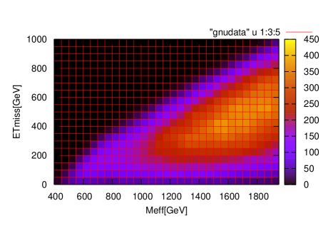
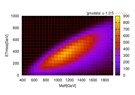
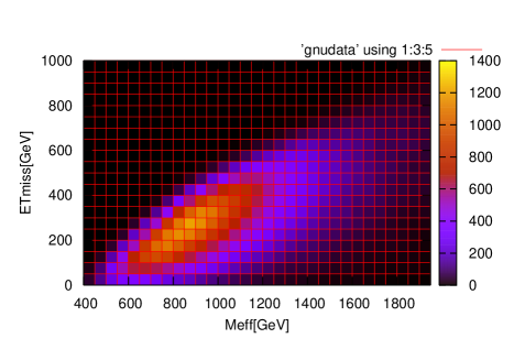
Figure 3: $M_{\rm eff}$ vs ${\not\!\!E}_{\rm T}$ distribution for the model B, with $M_{3}{\rm(GUT)}=650$ GeV, $\tan\beta=10$ and $R=0.1$ (top left), $R=40$ (top right) and $R=50$ (bottom) respectively.

This distribution can be understood as follows. Suppose we have events with two uncorrelated jets with energy $E_{\rm jet}=p_{\rm CM}$. The dominant part of the cross section is squark/gluino pair production near the threshold for our case, so if they decay directly into two jets and two LSPs, the event kinematics are indeed of this type up to the boost to the beam direction. We now calculate missing energy $E_{\rm miss}$ and effective energy $M{\rm(eff)}$ of the events. The momentum of the two jets and the missing momentum can be expressed as follows,

$$p_{1} = (p_{\rm CM},0,0,p_{\rm CM})$$ (24)

$$p_{2} = (p_{\rm CM},p_{\rm CM}\sin\theta,0,p_{\rm CM}\cos\theta)$$ (25)

$$p_{\rm miss} = (E_{\rm miss},-p_{\rm CM}\sin\theta,0,-p_{\rm CM}(1+\cos\theta))$$ (26)

where we take the direction of the $p_{1}$ momentum as $z$-axis and events are in $x$-$z$ plane. Then the missing energy $E_{\rm miss}$ and effective mass $M{\rm(eff)}$ are defined as

$$E_{\rm miss} = p_{\rm CM}\sqrt{2+2\cos\theta},$$ (27)

$$M{\rm(eff)} = 2p_{\rm CM}+E_{\rm miss},$$ (28)

where $M{\rm(eff)}$ ranges from $2p_{\rm CM}$ to $4p_{\rm CM}$.

The relation between ${\not\!\!E}_{\rm T}$ and $M_{\rm eff}$ is somewhat similar to that of $E_{\rm miss}$ and $M{\rm(eff)}$ as can be seen in Figure 3. For each plot ${\not\!\!E}_{\rm T}$ tends to be small when $M_{\rm eff}\sim 2p_{\rm CM}$, where $2p_{\rm CM}=1.36,0.95,0.7$ TeV for $R=0.1,40,50$, respectively. It increases linearly as a function of $M_{\rm eff}$ up to $M_{\rm eff}\sim 3p_{\rm CM}$, and the number of events reduces quickly beyond $M_{\rm eff}>4p_{\rm CM}$ . The relation indeed should be true when two particle are pair produced and each of them decays into a visible particle and an invisible particle at hadron collider.

On the other hand, for the dominant background coming from $W(Z)$+ $n$-jets or $t\bar{t}$ +$n$-jets, the ${\not\!\!E}_{\rm T}/M_{\rm eff}$ should be smaller than those of the signal. This is because the SM events have many other jet activities which are not associated with the missing momentum productions. The background comes from highly boosted events, where ${\not\!\!E}_{\rm T}$ is typically a fraction of the missing energy originated from high energy $W$, $Z$, and $t$. The canonical cut to reduce the SM background is ${\not\!\!E}_{\rm T}>0.2M_{\rm eff}$. If the background distribution in $M_{\rm eff}$ and ${\not\!\!E}_{\rm T}$ plane is significantly different from the signal distribution, one can improve the S/N by applying an improved cut in the plane rather than the simple cuts $M_{\rm eff}>400$ GeV and ${\not\!\!E}_{\rm T}>0.2M_{\rm eff}$ described in section 1. Because there are no background distribution study on the relation between $M_{\rm eff}$ and ${\not\!\!E}_{\rm T}$, we do not attempt to improve the cuts in following sections and use the cut given in section 1.

IV.2 The zero lepton channel

We now show the signal $M_{\rm eff}$ distributions for the degenerated model. We start our discussion from the $M_{\rm eff}$ distributions of the SUSY events without high $p_{T}$ leptons. This channel has been studied in TDR ; HP ; TOVEY with an emphasis on the model-independent reconstruction of the SUSY scale, as discussed in the previous subsection.

Figure 4: The $M_{\rm eff}$ distributions for non-lepton sample. The thick solid histogram is the background estimated in TDR . Solid and dashed histograms are signal distributions for $M_{3}{\rm(GUT)}=450$ GeV $R=0.1$ (MSUGRA), and $R=37$ (degenerate) in the left panel, and for $M_{3}{\rm(GUT)}=650$ GeV $R=0.1$ (MSUGRA) and $R=38$ (degenerate) in the right panel, respectively. All plots are normalized for $\int dt{\cal L}=10$ fb^-1.

In Figure 4, the signal distributions for the model A, with $M_{3}{\rm(GUT)}=450$ GeV and 650 GeV are plotted for $R\sim 0$ and $R\sim 37$. The signal distributions (solid and dashed histograms) are parallel to the background distribution (bars in the plots) beyond the peak of $M_{\rm eff}$ distribution. The difference appears only in the overall normalizations. As already discussed, this is because the signal distribution is determined mainly by the luminosity function, once $M_{\rm eff}\gg 2M_{\rm SUSY}$.

The background shown in the plots has a large uncertainty. The estimation has been made by the lowest order Monte Carlo generator ISAJET. The distribution is subjet to the scale uncertainty which is typically ${\cal O}$(30%). We also require at least 4 high $p_{T}$ jets, while the number of final state parton involved in the tree level diagram is much less than 4. The number of additional jets is estimated by parton shower (PS) approximation. The PS approximation is good to estimate distributions of jets collinear to the leading jets. Recently, several groups have emphasized the importance of the matrix element (ME) correction to the SM background processes. The matrix elements of the diagram involving $W,Z,t$ + $n$-partons are calculated by the generator devoted for the process with multi jets MANGANO ; RAINWATER ; Maltoni:2002qb . Experimental groups are also working to take into account the corrections, for example, in the ATLAS group TEV4LHC , the backgrounds from $(\bar{t}t,W,Z)$+$n$-jets are calculated up to $n=(3,6,6)$ respectively using ALPGEN MANGANO . After the inclusion of the ME corrections, the SM background is increased by a factor of 2$\sim$4 for $M_{\rm eff}>2$ TeV. Even in the highest bin in the plot, the expected background is above 1. This is caused by the increased high $p_{T}$ jets in the SM events. The improved background estimation is still preliminary and in the level of the lowest order, and subject of coupling scale uncertainty.

We find that the signal rate is the same order of the background rate for the degenerated parameters. If the uncertainty of the overall normalization of the background is 100%, no bound would be obtained from no-lepton channel by looking into $M_{\rm eff}$ distribution only. However, as we noted previously, the structure of the signal distribution may be visible over the background distribution in the $M_{\rm eff}$ and ${\not\!\!E}_{\rm T}$ plane.

IV.3 One lepton channel

The significant fraction of SUSY production gives rise to events with isolated leptons ($P_{T}>20$ GeV and $|\eta|<2.5$). We show the signal distribution for the model A in Figure 5. Here, we do not show the background distributions, because they are not given in previous literatures. In TEV4LHC , the distribution of the SM background is given, which is roughly 1/20 of the background of the zero lepton channel with a similar shape.

Figure 5: The signal $M_{\rm eff}$ distributions of one lepton events. The solid and dashed histograms correspond to model A, $R\sim 0$ (MSUGRA-like) and $R\sim 37$ (degenerated mass spectrum) respectively. $M_{3}{\rm(GUT)}=650$, 750, 850 GeV from left to right. All plots are normalized for $\int dtL=10$fb^-1.

Figure 6: The $M_{\rm eff}$ distributions for one lepton signal events for model B, $M_{3}{\rm(GUT)}=450$ GeV (left panel), $M_{3}{\rm(GUT)}=650$ GeV (right panel) and $\tan\beta=10$. Th solid histograms for $R=0.1$ (MSUGRA like) and dashed histograms for $R=55$ and $50$ respectively corresponding to degenerated mass spectrum. All plots are normalized for $\int Ldt=10$fb^-1.

Figure 7: The $m_{ll}$ and $m_{jll}$ distribution of signal for a degenerated SUSY point. $5\times 10^{4}$ SUSY events are generated for model A, $M_{3}$(GUT)$=450$ GeV, $\tan\beta=10$ and $R=37$.

The histograms in Figure 5 show signal distributions for $M_{3}{\rm(GUT)}=650$ GeV, $750$ GeV, $850$ GeV from left to right, and $R\sim 0$ for solid line and $R=38,37,37$ for dashed lines, respectively. As can be seen in Table 3, the minimum mass difference is smaller for the model B than that for the model A, because the higgsino mass $\mu$ is higher. Because of the degeneracy, the signal is more suppressed as can be seen in Figure 6 where we take $M_{3}{\rm(GUT)}=450$ GeV (left) and $650$ GeV (right), $R=55$ and $50$ (dashed histograms), respectively. Overall normalization of the signal above $M_{\rm eff}>1.6$ TeV reduces by a factor of 1/10 for for model B $M_{3}{\rm(GUT)}=650$ GeV (Figure 6, right panel) compared to the model A (Figure 5, left panel) for most degenerate points. We conclude that one lepton signal is not accessible at the most degenerated points by looking into $M_{\rm eff}$ distribution alone, assuming that SM background in the one lepton channel in TEV4LHC , and a factor 2$\sim$ 3 uncertainty, even though the SUSY scale is relatively small for this point, $m_{\tilde{g}}=1.48$ TeV The mass reach at the LHC will be revisited again in section 4.5.

IV.4 Two lepton channel

For the model A, there are significant two lepton events in the $\mu\sim M_{1}$ region because $\tilde{l}$ is lighter than the $\widetilde{W}$-like neutralino. We show the $m_{ll}$ and $m_{jll}$ distribution for the model A, with $M_{3}{\rm(GUT)}=450$ GeV and $R=37$ in Figure 7. Here we require that one of the two isolated leptons has $p_{T}>20$ GeV and the other has $p_{T}>10$ GeV. We also apply the standard cuts described in section I. The relevant mass spectrum for the most prominent endpoints are $m_{\tilde{u}_{R}}=901$ GeV, $m_{\tilde{d}_{R}}=869$ GeV, $m_{\tilde{\chi}^{0}_{2}}=554$ GeV, $m_{\tilde{\chi}^{0}_{1}}=499$ GeV, and $m_{\tilde{e}_{R}}=524$ GeV. The predicted $m_{ll}$ edge and $m_{jll}$ endpoint for the decay chain $\tilde{q}_{R}\rightarrow\tilde{\chi}^{0}_{2}\rightarrow\tilde{l}_{R}\rightarrow\tilde{\chi}^{0}_{1}$ is $m_{ll}=54.9$ GeV and $m_{jll}=308$ GeV, respectively, consistent with Figure 7. The edges and endpoints of other cascade decays are also visible in the plots.

To select the jet from $\tilde{q}$ decays, we have taken the one of two most highest $p_{T}$ jets with smaller $m_{jll}$. If mass difference between $m_{\rm\tilde{q}}$ and $m_{\tilde{\chi}^{0}_{1}}$ is smaller, we may found the smaller probability to find correct jets that arise from $m_{\tilde{q}}$ decay. We do not observe such effect in Figure 7.

The number of accepted events $N_{i}$ (where $i$ denotes number of isolated leptons with $p_{T}>20$ GeV and $|\eta|<2.5$) for this point are $N_{0}=11229$, $N_{1}=5167$, $N_{2}=2645$ for $5\times 10^{4}$ generated events (corresponding to $\sim$ 20 fb^-1) . Number of two lepton events below the dominant edge is 2933 after the background subtraction. Because $M_{\rm eff}$ distribution of the one lepton channel is not very prominent over the background, SUSY particles may be discovered in the two lepton channel for the degenerate region.

Note that for the most degenerated SUSY spectrum, we have $M_{1}\sim M_{2}\sim\mu$ so that all neutralinos are highly mixed. In such situation, dominant source of $\tilde{\chi}^{0}_{2}$ is $\tilde{q}_{R}$, because $\tilde{q}_{L}$ has significant decay branching ratios into charginos. It is worth to point out that the relative weight of the decays $\tilde{q}_{L(R)}\rightarrow\tilde{\chi}^{0}_{2}\to\tilde{l}_{L(R)}$ may be studied by looking into the charge asymmetry in $m_{jl}$ distributions, $A\equiv(m_{jl^{+}}-m_{jl^{-}})$ $/(m_{jl^{+}}+m_{jl^{-}})$ BARR ; GOTO . The charge asymmetry comes from the polarization of $\tilde{\chi}^{0}_{2}$ arising from $\tilde{q}$, however as discussed in WEBBER , the effect tends to be suppressed if sparticle masses are degenerated.

For the model B, the decay of $\tilde{\chi}^{0}_{i}$ into sleptons are closed for any value of $R$. For $M_{3}{\rm(GUT)}=450$ GeV and $R=40$, we have $N_{0}=13433$, $N_{1}=4412$, $N_{2}=642$ for $5\times 10^{4}$ generated events. While $N_{0}$ and $N_{1}$ is about same as that of the model A, $N_{2}$ is reduced by a factor of 4. In addition no significant events with opposite sign same flavor leptons are seen after the subtraction of $e^{\pm}\mu^{\mp}$ events.

IV.5 Discovery potential in one lepton channel

In MSUGRA, the signal $M_{\rm eff}$ distribution is clearly harder than the background. Especially, one can see the increase of the signal towards its peak, where the background is negligible. If the total $M_{\rm eff}$ distribution shows a bump or a clear change in the power behavior, one may claim discovery of SUSY particles without precise understanding of the background distribution.

On the other hand, when SUSY mass spectrum is degenerated, the peak of the signal distribution shifts to a lower position where the background may be $\sim$10 times higher. The signal distribution shows a similar power low behavior for $M_{\rm eff}>M^{\rm peak}_{\rm eff}$ as can be seen in Figure 4. The bump structure may not be detected and precise understanding of the background would be required. Searching edges in $m_{ll}$ distribution from the decay $\tilde{\chi}^{0}_{2}\rightarrow$ $\tilde{l}\rightarrow\tilde{\chi}^{0}_{1}$ may become more important, however, as we have discussed already, the signal rate is model dependent. We do not consider the possibility to improve S/N ratio by selecting signal region $M_{eff}$ vs ${\not\!\!E}_{\rm T}$ in this subsection.

Table 4 shows the number of signal events after the cut for $M_{\rm eff}$ intervals for $5\times 10^{4}$ generated event (upper row) and number of events for 10 fb^-1 (lower row) for both model A and model B. We take a moderate value of $M_{3}{\rm(GUT)}=650$ GeV for the Table, which corresponds to $m_{\tilde{g}}\sim 1.4$ TeV.

$M_{\rm eff}$(TeV)	0.8-1.2	1.2-1.6	1.6-2.0	2.0-2.4	2.4-3.2	3.2-4.0	$\sigma$	$2p_{\rm CM}$(TeV)
model A
$R=0.1$	448	905	1267	999	568	69	0.252pb	1.35
	22.5	45.6	63.9	50.3	28.8	3.4
10	752	1201	1378	896	483	59	0.245pb	1.29
	36.8	58.8	67.4	43.8	23.9	2.9
20	813	1421	1319	676	293	17	0.248pb	1.20
	40.3	70.5	65.4	33.7	14.5	0.8
30	1246	1691	1018	336	95	9	0.267pb	1.04
	66.6	90.4	54.4	18.0	5.1	0.5
40	2446	2337	758	212	63	9	0.314pb	0.87
	152.3	145.5	47.2	13.2	4.0	0.6
50	882	960	529	198	65	4	0.457pb	0.90
	80.7	87.8	48.4	18.1	5.9	0.4
55	173	249	175	71	26	5	0.666pb	0.94
	23.0	33.2	23.2	9.5	3.5	0.7
model B
$R=0.1$	450	1108	1405	1192	784	96	0.206pb	1.42
	18.6	45.7	57.9	49.2	32.3	4.0
10	649	1267	1585	1145	654	67	0.187pb	1.38
	24.3	47.4	59.3	42.8	24.5	2.5
20	836	1528	1645	962	432	42	0.174pb	1.31
	29.1	53.2	57.2	33.5	15.0	1.5
30	943	1838	1362	561	217	26	0.165pb	1.2
	31.2	60.7	45.0	18.5	7.2	0.9
40	1711	1591	711	184	86	4	0.158pb	0.99
	54.0	50.2	22.4	5.8	2.7	0.1
50	2428	803	215	67	25	5	0.154pb	0.73
	74.9	24.8	6.6	2.1	0.8	0.2

Table 4: The number of events per $M_{\rm eff}$ bins in model A and model B. The upper rows show the events for 50000 events in our simulations, and lower rows show the event per 10 fb^-1. $M_{3}{\rm(GUT)}=650$ GeV.

In the MSUGRA limit $(R\sim 0)$, the background rate is negligible in the signal region. The number of events in $M_{\rm eff}>2.5$ TeV is greater than 10 for $R<20$, where the number of background events would be around 1 according to TEV4LHC . However, the signal rate is reduced by more than a factor of $4$ for $R>30$ compared to that at $R\sim 0$. Another important question is if we have a flatter power spectrum in a certain $M_{\rm eff}$ region. The number of background events is reduced steeply $M_{\rm eff}$ bins in Figure 4, while we have nearly flat signal distribution between $1.2$-$2.4$ TeV for MSUGRA-like ($R\sim 0$) points. The ratio between the signal in the bins $N(1.6{\rm TeV}<M_{\rm eff}<2.0{\rm TeV})$ and $N(2.0{\rm TeV}<M_{\rm eff}<2.4{\rm TeV})\sim 3:1$ for $R=30,40$ for the model A and for $R=30,40,50$ for the model B, therefore the power law for the signal is similar to that of background in Figure 4 . We can describe the discovery potential in terms of the mass degeneracy rather than $R$. In the Table 4, $2p_{\rm CM}$ ranges from $1.4\sim 0.7$ TeV. ($M_{\tilde{q}}=1.4$ TeV ). Once $2p_{\rm CM}$ reduces below 1 TeV, 70% of $M_{\tilde{q}}$, the separation between signal and background are not good in $M_{\rm eff}$ distributions. Good understanding of the background distribution and the detector effect is required to exclude the model in early stage of LHC runs $\int dt{\cal L}=10$fb^-1.

A factor 2 decrease of the signal is found for the model A between $R=50$ and $R=55$. In this model, squark mass decreases as $R$ increases. While the production cross section increases as ${\tilde{q}}$ gets lighter, the masses of heavier neutralino and chargino increase. They are heavier than $\tilde{q}$ at $R=55$, so that they would not be produced from $\tilde{q}$ decay at all. The lighter neutralinos and charginos are still lighter than $\tilde{q}$ but they are degenerated, so that only soft leptons are produced from the decay. The two lepton signal is also suppressed for this model point. This is an example that the rate of signal events with lepton is model dependent.

The tendency of the signal reduction is same for the higher mass spectrum. The luminosity needed to discover the SUSY signal is larger at the degenerated SUSY points. For example, the production cross section is $43.6$ fb for the model A with $M_{3}{\rm(GUT)}=850$ GeV and $R=0$, and 15.1 events/10 fb^-1 is expected in the region $2.4$ TeV $<M_{\rm eff}<4$ TeV, which may be enough to claim the discovery. On the other hand, for $R=37$ only 3.8 events/10 fb^-1 is expected, excluding the possibility of discovery with low luminosity.

V discussion and conclusion

In this paper, we study the discovery potential of minimal supersymmetric models with degenerated mass spectrum at the LHC. Such parameter regions have not been systematically studied in the past. SUSY studies have been mainly performed in the models where gluino and squark are significantly heavier than the LSP, i.e. in the MSUGRA model, gauge mediation model, and so on.

We do not study the general MSSM model here, but take mixed modulas anomaly mediation (MMAM) models, which are parametrized by $R\propto F_{C}/F_{T}$, $\tan\beta$, and $M_{3}{\rm(GUT)}$. The parameter $R$ is the ratio of the $F$ terms of the volume modulas $T$ in KKLT model and the compensator field $C$ in $N=1$ MSUGRA. This parameter $R$ gives us one parameter description from the MSUGRA-like mass spectrum, where $M_{3}\gg M_{1}$, to (moderately) degenerated mass spectrum. The models we have studied include the MSSM points where $m_{LSP}/M_{\tilde{q},\tilde{g}}\sim 0.7$.

When sparticle mass spectrum is degenerated, energy of a particle from squark and gluino decays is small relative to the mass scale. This is reflected in the distributions of the first $p_{T}$ jet, ${\not\!\!E}_{\rm T}$ and $M_{\rm eff}$. They tend to peak at smaller values than MSUGRA prediction for the same gluino and squark masses. The background from the SM processes increases rapidly for such low $p_{T}$ and low $M_{\rm eff}$ region, therefore, the SUSY signal has to compete with large background. Indeed, the signal and background $M_{\rm eff}$ distributions are quite similar for degenerated parameters we have studied. We find the $S/N$ ratio can be far below 1 for our most degenerated parameter points. Nevertheless, we found the signal distribution of degenerated SUSY mass spectrum show special universal pattern in $M_{\rm eff}$ and ${\not\!\!E}_{\rm T}$ plane. This may help to determine the appropriate signal region and discriminate signal from background better.

The discovery potential at the degenerated points therefore depends on our knowledge on the background distribution. The main background source to the SUSY productions is multijet final states involving $W$, $Z$ and $t$. There are significant improvements in the lowest order estimation of the background recently; Matrix element corrections of the backgrounds are now included. Theoretical uncertainty comes from matching between parton shower approximation and matrix corrections, and higher order QCD corrections (scale uncertainty).

Experimentally backgrounds are partly estimated by the experimental data itself. For example, overall normalization of dominant $t\bar{t}$ background can be determined by looking into the events with low ${\not\!\!E}_{\rm T}$, where contamination of the SUSY events are small. For the degenerated mass spectrum, however, such calibration may also be affected. Note that the background estimation in the SUSY signal region require extrapolation using Monte Carlo, while there is a contamination in the region for the calibration in non-trivial manner for degenerated SUSY mass spectrum. We look into ${\not\!\!E}_{\rm T}$ distribution and find that the number of events with ${\not\!\!E}_{\rm T}<200$ GeV is increased by factor of $2$ for our most degenerated point (the model B with $R=55$, $M_{3}{\rm(GUT)}=450$ GeV) from MSUGRA limit ($R=0.1$).

Even with the uncertainty discussed above, the discovery of supersymmetry in MSUGRA models would not be a problem up to $\sim$ 2 TeV region. However, as we have discussed in this paper, this is not the case even for moderately degenerated SUSY parameters in mixed modulas anomaly mediation model. We stress the importance to include the background and its uncertainty to perform SUSY discovery and parameter studies for degenerated or general MSSM mass spectrum, while we find that they tend to be ignored in recent studies TATA ; KANE .

References

- (1) S. P. Martin, “A supersymmetry primer,” arXiv:hep-ph/9709356.
- (2) ATLAS Collaboration, ATLAS detector and physics performance Technical Design Report, CERN/LHCC 99-14/15 (1999).
-
(3)
I. Hinchliffe, F. E. Paige, M. D. Shapiro, J. Soderqvist and W. Yao,
Phys. Rev. D 55, 5520 (1997)
[arXiv:hep-ph/9610544].
H. Bachacou, I. Hinchliffe and F. E. Paige, Phys. Rev. D 62, 015009 (2000) [arXiv:hep-ph/9907518]. - (4) arXiv:hep-ph/0410364. Section 5.1.2 ”A detailed analysis of the measurement of SUSY masses with the ATLAS detector at the LHC
- (5) S. Kachru, R. Kallosh, A. Linde and S. P. Trivedi, Phys. Rev. D 68, 046005 (2003) [arXiv:hep-th/0301240].
- (6) K. Choi, K. S. Jeong and K. i. Okumura, JHEP 0509, 039 (2005) [arXiv:hep-ph/0504037].
- (7) A. Falkowski, O. Lebedev and Y. Mambrini, JHEP 0511, 034 (2005) [arXiv:hep-ph/0507110].
- (8) M. Endo, M. Yamaguchi and K. Yoshioka, Phys. Rev. D 72, 015004 (2005) [arXiv:hep-ph/0504036].
- (9) T. Plehn, D. Rainwater and P. Skands, arXiv:hep-ph/0510144,
- (10) S. Asai, talk in 4th TEV4LHC, Oct 20 -22, 2005 at FermiLab. http://conferences.fnal.gov/tev4lhc/
- (11) M. L. Mangano, M. Moretti, F. Piccinini, R. Pittau and A. D. Polosa, JHEP 0307, 001 (2003) [arXiv:hep-ph/0206293]. See also http://mlm.home.cern.ch/mlm, [Merging matrix element and shower]
- (12) H. Baer, F. E. Paige, S. D. Protopopescu and X. Tata “ISAJET 7.48: a Monte Carlo event generator for , , and reactions”, hep-ph/0001086.
- (13) G. Corcella et. al., JHEP 01 (2001) 010, [arXiv:hep-ph/0011363].
- (14) http://www.hep.phy.cam.ac.uk/ richardn/HERWIG/ISAWIG/
- (15) http://www.physics.ucdavis.edu/ conway/research/software/pgs/pgs4-general.htm
- (16) E. Richter-WAS, D. Froidevaux and L. Poggioli, ”ATLFAST 2.0:a fast simulation package for ATLAS”, Tech. Rep.ATL-PHYS-98-131(1998)
- (17) B. C. Allanach et al., in Proc. of the APS/DPF/DPB Summer Study on the Future of Particle Physics (Snowmass 2001) ed. N. Graf, Eur. Phys. J. C 25 (2002) 113 [eConf C010630 (2001) P125] [arXiv:hep-ph/0202233].
- (18) D. R. Tovey, Eur. Phys. J. directC 4, N4 (2002).
- (19) F. Maltoni and T. Stelzer, JHEP 0302, 027 (2003) [arXiv:hep-ph/0208156].
- (20) A. J. Barr, Phys. Lett. B 596, 205 (2004) [arXiv:hep-ph/0405052].
- (21) T. Goto, K. Kawagoe and M. M. Nojiri, at the CERN Large Hadron Collider,” Phys. Rev. D 70, 075016 (2004) [Erratum-ibid. D 71, 059902 (2005)] [arXiv:hep-ph/0406317].
- (22) J. M. Smillie and B. R. Webber, JHEP 0510, 069 (2005) [arXiv:hep-ph/0507170].
- (23) H. Baer, E. K. Park, X. Tata and T. T. Wang, arXiv:hep-ph/0604253.
- (24) N. Arkani-Hamed, G. L. Kane, J. Thaler and L. T. Wang, arXiv:hep-ph/0512190.