Review of Theoretical Status:
the Long and Short of High Energy Jets

Abstract

High energy jets and their associated event shapes provide a window into the transition between elementary and composite degrees of freedom in quantum chromodynamics. This talk reviews some methods and a few principles that have led to progress in this area.

I Motivation: QCD, the Protean Theory

Why fuss over quantum chromodynamics? Why not simply leave a true theory alone, except perhaps to derive it from some underlying physics beyond the standard model? The Large Hadron Collider, of course, plans to put QCD to work in coaxing new states out of virtuality and into plain sight. Another enduring challenge in contemporary science, however, is to bridge the gap between a reductionist description of nature in “elementary” terms, and an effective description in terms of “emergent” excitations. Quantum chromodynamics is a perfect testing ground for such a program. In the words of Shakespeare’s Duke of Gloucester, it “can add colors to the chamelion/Change shapes with Proteus for advantages” [Henry VI, part III], and out it emerge a host of effective theories at varying length scales. Quantum chromodynamics spans the chasm between the theory of Yang and Mills at high energies and that of Yukawa at low energies, not to mention nuclei, and the description of strongly interacting matter at varying temperatures and densities. The only problem is that these aspects of the theory can very difficult to analyze with our current tools.

The current era of high energy colliders brought the theory of QCD into being. This required a temporary step back from the study of the fine structure of final states, to their gross properties, which can encode events at short distances. Before this was realized, however, the detailed structure of final states were front and center. In this context, Yang observed in 1969 that yang69 “…in the midst of enormous complexities there are very striking characteristics exhibited by high energy collisions …A number of ideas, models etc. been introduced …ideas behind these models are not always mutually exclusive, especially since none of them is completely precisely defined.” In many ways, this describes our current situation. Now we have a theory, QCD, and we are ready to turn our attention back to the individual particles produced by the strong interactions. We understand some of these regularities as keys to the protean transition from weak to strong coupling. Our challenge is to use these characteristics as guides for progress from models to principles. We have a very long way to go before we can truly bridge this gap, but we have made some halting progress. And in a sense that is the subject of our workshop.

II Power Corrections from Perturbation Theory: the OPE and a Massive Gluon

We begin with a compressed intellectual history of observations that make it possible to derive power corrections from perturbation theory. This subject is intimately related to the evolution of the QCD coupling. It begins most naturally with fully inclusive cross sections, which can be related to Green functions in Euclidean space.

II.1 Discovering the operator expansions

Our discussion begins with the work of Mueller mueller85 , in 1985. ’t Hooft thooft74 had previously introduced the concept of renormalons, applied to Euclidean Green functions, but it was Al who made the crucial step into Minkowski space, by exploiting the unitarity relation

$$\sigma_{\rm tot}^{{\rm e}^{+}{\rm e}^{-}}={(4\pi\alpha)^{2}\over Q^{2}}\,{\rm Im}\;\pi(Q^{2})$$ (1)

between the total cross section for lepton-positron annihilation and the imaginary part of the time-ordered products of currents

$$\pi(Q^{2})=\left({-i\over 3Q^{2}}\right)\;\int d^{4}x\;{\rm e}^{-iq\cdot x}\langle 0|Tj^{\mu}(0)j_{\mu}(x)|0\rangle\,.$$ (2)

This is the optical theorem, illustrated in Fig. 1. It provides a link between a short-distance dominated quantity, the self-energy of an off-shell vector boson (photon, Z) and the annihilation cross section, which of course is the (inclusive) result of measurements at arbitrarily large times.

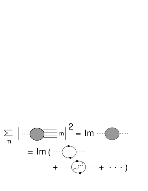
Figure 1: Graphical representation of the optical theorem as applied to leptonic annihilation through a vector boson.

The important relationship between the operator product expansion for the product of currents

$$\langle 0|j^{\mu}(0)j_{\mu}(x)|0\rangle={1\over x^{6}}\;{\tilde{C}}_{0}(x^{2}\mu^{2}),\alpha_{s}(\mu))\ +{1\over x^{2}}\;{\tilde{C}}_{F^{2}}(x^{2}\mu^{2},\alpha_{s}(\mu))\langle 0|F_{\mu\nu}F^{\mu\nu}(0)|0\rangle+\dots\,,$$ (3)

and the total cross section was already well-established. In the method of QCD sum rules qcdsum , the first term of this expansion is interpreted as finite-order perturbation theory, while additional terms are computed by introducing new parameters, the condensates, in an extension of the perturbative series. The consistency between $\pi(Q)$ computed in this way and experiment leads to many predictions, always keeping in mind that the values of the nonperturbative parameters depend on the order of perturbation theory.

On the other hand, if we stick to perturbation theory at the outset, we find that the perturbative expansion for the function $\pi(Q)$ is completely well-defined and finite order-by-order, a property called infrared safety:

$$\pi(Q)\sim C_{0}(Q^{2}/\mu^{2},\alpha_{s}(\mu))=\sum_{n=0}^{\infty}c_{0}^{(n)}(Q^{2}/\mu^{2})\;\alpha_{s}^{n}(\mu)\,,$$ (4)

with $\mu$ the renormalization mass. It would seem then, that perturbation theory knows only about the leading power coefficient, $C_{0}$. So what about $\tilde{C}_{F^{2}}$ and the rest of the coefficients? In fact, although the other terms are not predicted by QCD perturbation theory, their presence is implicit in it. The reason is that the series for $C_{0}$ doesn’t converge.

To see how this nonconvergence comes about, we can consider a point in the loop momentum space of any diagram for $\pi(Q)$, where the momentum $k$ carried by some gluon vanishes in all four components. In the language of gs78 , the subspace where this happens is a “pinch surface”, which cannot be avoided by deforming the contours of loop momenta. The configuration is illustrated in Fig. 2.

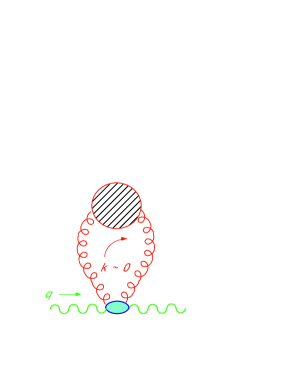
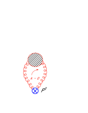
(a)                                                             (b)

Figure 2: Momentum configuration related to renormalons and the operator product expansion.

As we integrate over the loop momentum $k$, the invariant $k^{2}$ varies. As we shall see, it is sometimes convenient to think of this as a “gluon mass”. In the figure we show a gluon self-energy, which in general includes a series of one-particle irreducible diagrams. Each such diagram behaves at lowest order as a (negative) constant times $\alpha_{s}\,\ln(k^{2}/\mu^{2})$. Thus, a typical term in the perturbative expansion of the gluon self energy produces a $k$ integral that may be approximated for $0<k<Q^{2}$ by

$$C_{0} \sim (1/Q^{4})\;\alpha_{s}^{n}\,\int_{0}^{Q^{2}}dk^{2}k^{2}\;\ln^{n}(k^{2}/\mu^{2})\sim(1/2)\left(\alpha_{s}/2\right)^{n}\;n!\,.$$ (5)

Dimensional counting plus the requirements of gauge invariance ensure that the integrand vanishes as $k^{2}/Q^{2}$ for $k^{2}\to 0$, which corresponds dimensionally to the operator $F^{2}$ in Eq. (3). Indeed, we can think of $F^{2}$ as an operator in an effective theory for soft gluons where all short-distance degrees of freedom at scale $Q^{2}$ have been “integrated out”, and there are no on-shell partons to produce collinear singularities.

We can now imagine separating the full integral for $C_{0}$ into the sum of two terms, one in which no gluons have vanishing momentum and another in which we group the neighborhoods of all the points $k=0$. For a generic diagram this would be an arduous task, but one that can clearly be accomplished in a finite number of steps. The schematic result is

$$C_{0}=C_{0}^{({\rm reg})}+{C_{0}^{({\rm pinch})}}+{{\cal O}(Q^{-6})}\,,$$ (6)

where in the second, “pinch” term, Mueller showed that to the relative power $Q^{-6}$ all the logarithms can be incorporated into the running coupling evaluated at the gluon “mass”,

$$C_{0}^{({\rm pinch})} = H(Q){\int_{0}^{\kappa^{2}}dk^{2}k^{2}\;\alpha_{s}(k^{2})}$$ (7)

$$= H(Q){\int_{0}^{\kappa^{2}}dk^{2}k^{2}\ {\alpha_{s}(Q^{2})\over 1+\left({\alpha_{s}(Q^{2})\over 4\pi}\right)\beta_{0}\ln(k^{2}/Q^{2})}}$$

$$= H(Q){\int_{0}^{\kappa^{2}}dk^{2}k^{2}\;{4\pi\over\beta_{0}\ln(k^{2}/\Lambda^{2})}}\,,$$

with $\kappa\ll Q$ a new factorization scale, which we introduce to separate these “soft corners” of momentum space. The function $H(Q)$ represents the short-distance-dominated factors left over (the shaded region in Fig. 2(a)). We will call such a reorganization of perturbation theory an “internal resummation” gsth2002 , one in which all logarithmic behavior in $\int f(\alpha_{s}(k^{2}))$ has been absorbed into the running coupling. We also see that, because the perturbative running coupling is undefined at the QCD scale $\Lambda$, an internal resummation alone does not produce a well-defined, finite result.

Now, here’s the operator product expansion: soft integrals in $C_{0}^{({\rm pinch})}$ and for the perturbative expansion $\langle 0|F^{2}|0\rangle$ are identical, something that we can see by comparison of (a) and (b) in Fig. 2 once we realize that the factor of $k^{2}$ near the pinch surface corresponds to the local vertex $F^{2}$. At this point we invoke what I like to call an “axiom of substitution”, also known as “matching”. That is, we postulate that the true behavior of the two-point function is found by systematically removing the soft corners of integrals in perturbation theory, and replacing them with power corrections in the form of matrix elements that have the same integrals in the same soft corners. As we have argued, such a process will be consistent with the operator product expansion (in this case), and we write

$${C_{\rm PT}\over Q^{4}}\rightarrow C_{\rm PT}^{\rm reg}\left(\frac{Q^{2}}{\mu^{2}},\frac{\kappa}{Q},\alpha_{s}(Q)\right)+C_{F^{2}}(Q,\kappa)\ {{\alpha_{s}\langle 0|F^{2}(0)|0\rangle(\kappa)\over Q^{4}}}\,.$$ (8)

In summary, the nonconvergence of perturbation theory implies the need for new (infrared) regularization. The cost of introducing such a regularization is that the theory requires a new nonperturbative parameter (i.e., $\langle F^{2}\rangle$). By the same token, the benefit of this procedure is to recognize the necessity of this same parameter (i.e., $\langle F^{2}\rangle$), which emerges from perturbation theory. Such an analysis is possible, and indeed necessary, whenever there is an internal resummation, an integral of the form $\int f(\alpha_{s}(k^{2}))dk^{2}$ to all logs, for some funnction $f$ of the running coupling.

Of course, we may start from an alternative viewpoint, assuming the OPE from the beginning. In this case, we interpret the matching above as a cancellation of high-order corrections between leading-power perturbation theory and the operator matrix elements. Whichever way we interpret this correspondence, the actual values of nonperturbative parameters will depend on the definition of perturbation theory. The method of effective charges, discussed by Maxwell effcharge at this meeting, shows how flexible the values of these parameters can be!

Yet another common method is in terms of a Borel transform mueller85 ; thooft74 , which we can see emerge from our analysis above. To do so, we may change variables in Eq. (7),

$$b\equiv 2\alpha_{s}(Q^{2})\ln(Q^{2}/k^{2})\,,$$ (9)

in terms of which $C_{0}$ becomes

$$C_{0}^{\rm pinch}\left(\alpha_{s}(Q)\right)={1\over 2}\;H(Q)Q^{4}\;\int_{0}^{\infty}db\;e^{-b/\alpha_{s}(Q)}{1\over 1-{\beta_{0}\over 8\pi}\;b}\,,$$ (10)

illustrated in Fig. 3. The explicit pole in the integrand is none other than the pole in the perturbative running coupling. Here, it should be regarded as an ambiguity in the integral at the value $b=8\pi/\beta_{0}$ of the transform variable. Any finite redefinition of the integral to make it unambiguous comes in only at the level of $Q^{-4}$ relative to the leading contribution from the transform.

                                            

Figure 3: The Borel plane interpretation of Eqs. (7) and (10).

It is certainly worth noting that such “infrared renormalon” power corrections are not the only possible sources of nonperturbative corrections. The very existence of solutions to the classical equations of motion, such as instantons, implies nonconvergent behavior of the perturbative series solutions . Another potential source of nonperturbative corrections are ultraviolet renormalons, poles on the negative real axis of the $b$-plane uvrenorm . While these corrections may well exist, phenomenological evidence appears at present to be associated with the infrared effects, and in the remainder of this talk I will restrict my discussion to the latter.

III Semi-inclusive cross sections

The ideas described above took a big step forward in the mid-1990s, with applications to semi-inclusive cross sections. The operator product expansion applies only to a very small set of observables, but there is a much larger class of observables that are infrared safe, that is, calculable order-by-order in perturbation theory with finite coefficients. As for the example above, we don’t expect the resulting series to be convergent, but once again we may ask whether that nonconvergence could be set to our advantage. My references below to the work that grew out of this realization will be of necessity incomplete, but at this point I can mention two very useful reviews, by Beneke and Braun BBpowerreview and by Dasgupta and Salam DSeventreview .

III.1 Internal resummation and power corrections

For many infrared safe quantities, we can find a resummation of logarithms, which can be generated from an integral over the running coupling, appearing in a form similar to (7) above, $(1/Q^{2})\int_{0}^{Q^{2}}f(\alpha_{s}(k^{2}))dk^{2}$, for some $f$ and some pertubative scale $Q$. Expanded back into a power series in a fixed coupling like $\alpha_{s}(Q)$, all integrals are finite, which is just a restatement that such an expression is consistent with infrared safety. In the light of our discussion above, however, we may be tempted to interpret the ambiguity in defining the lower end of such an integral, $0\geq k^{2}\leq\Lambda_{\rm QCD}$, as signaling the presence of a nonperturbative power correction. The approach just described has indeed been pursed by many investigators for many infrared safe processes earlypower ; Webber94 ; NasonSeymour95 . In some sense it is the simplest viewpoint to take, and one may apply it wherever the running coupling is encountered in an integral. As we shall see shortly, it is a particularly natural approach for resummed cross sections.

At the same time, to increase confidence in our interpretation, we might want to require that such an expression organize “all logs”, that is, in our terminology above, that it be an “internal resummation”. I will come back to this later.

III.2 Massive gluons and dispersive couplings

A very influential line of reasoning takes a viewpoint related to internal resummation, with a focus on the “massive gluon” introduced above. At least one current of this reasoning began with the observation that particle masses give generic $m/Q$ corrections to event shapes (see below). For the event shape thrust this observation goes back at least to R. Basu in 1984, for the specific case of the b quark Basu84 . In 1994, Webber Webber94 proposed using the gluon “mass” in event shapes, generalizing the work of Bigi et al. in heavy quark physics Bigietal . This approach in turn can be given precise realization by “large-$\beta_{0}$” or “dressed gluon” dga ; Berger04 approximations, which employ specific models for gluon self-energy diagrams. These and related ideas remain quite useful in organizing power correcctions.

In a sense, the apotheosis of the massive gluon is found in the conjecture of Dokshitzer, Marchesini and Webber (DMW) that the QCD coupling has a “dispersive” structure, conveniently written in terms of functions $\rho$ and $\alpha_{\rm eff}$ as dispersive

$$\alpha_{s}(k^{2})=-\int_{0}^{\infty}\frac{d\mu^{2}}{\mu^{2}+k^{2}}\ \rho_{s}(\mu^{2})\,,\quad\rho_{s}(\mu^{2})=\frac{d}{d\ln\mu^{2}}\alpha_{\rm eff}(\mu^{2})\,.$$ (11)

Applied to QED, the function $\rho(\mu^{2})$ is just the gauge-invariant photon self-energy, which is essentially the QED perturbative running coupling. The generalization to QCD in (11) defines a formalism that can be implemented at fixed order, but whose extension to all orders has not, to my knowledge, been fully explored. This apparent limitation, however, may not be that restrictive, especially if one takes the viewpoint that $\alpha_{s}(\mu^{2})$ itself behaves much more smoothly at low scales than the exptrapolation of its perturbative description smoothas .

With this possibility in mind, DMW proposed a template for any infrared safe observable $F$, which can be implemented with an NLO analysis. Consider, then, an arbitrary process dressed by a single gluon that carries loop momentum $k$, as in the example above. After an integration by parts, $F$ can be put in the form

$$F(x,Q)=-\int_{0}^{\infty}\frac{d\mu^{2}}{\mu^{2}}\,\alpha_{\rm eff}(\mu)\,\frac{d{\cal F}(x,Q,\mu)}{d\mu^{2}}\,,$$ (12)

with the function ${\cal F}(x,Q,\mu)$ the NLO underlying short-distance sub-process, and $\mu$ the variable “mass” of the gluon that emerges from this subprocess. For this expression to be meaningful, it is only necessary that ${\cal F}$ remain finite for $\mu^{2}\to 0$, and an expansion in $\mu/Q$ organizes power corrections, much as for the example from $\rm e^{+}e^{-}$ annihilation above.

The next step is to approximate the “effective” running coupling $\alpha_{\rm eff}$ in (12) as the sum perturbative and nonperturbative terms. Naturally, the definition of the latter depends on the former. The very simplest perturbative running coupling is a fixed coupling, say $\alpha_{s}(Q^{2})$, dressed by one or two terms from the beta function. In event shapes, discussed below, certain NLO effects are naturally taken into account in a “MC” or “physical” scheme for the coupling, related to the familiar $\overline{\rm MS}$ scheme by

$$\alpha_{s}=\alpha_{s}^{\rm\overline{MS}}\left(1+\frac{\alpha_{s}}{2\pi}\,K\right)\,,\quad K=C_{A}\left(\frac{67}{18}-\frac{\pi^{2}}{6}\right)-\frac{5}{9}n_{f}\,.$$ (13)

In this way, the Landau pole is simply discarded. The idea is that well above the Landau pole (say at the one GeV level), the perturbative running coupling should be replaced by a smooth nonperturbative function, that DMW call $\delta\alpha_{\rm eff}$. This function is a priori unknown. In Eq. (12), however, it will appear in universal moments, such as

$$A_{2p}=\frac{C_{F}}{2\pi}\int_{0}^{\infty}\frac{d\mu^{2}}{\mu^{2}}\ \mu^{2p}\,\delta\alpha_{\rm eff}(\mu^{2})\,,$$ (14)

where the powers (and sometimes logarithms) of the “gluon mass”, $\mu$, come from the expansion of ${\cal F}$. Phenomenological studies of power corrections then make it possible to determine these moments and, by comparing different processes, to check their universality. This procedure has been applied to many infrared safe observables. For inclusive processes, it reproduces the operator product expansion (with perhaps some extra assumptions about the vanishing of certain of the moments $A_{q}$), but its most important implications are for semi-inclusive processes, to which the operator product expansion does not directly apply.

III.3 Event Shapes and the Milan Factor

Let’s recall that event shapes, $e(N)$ are numbers that depend on energy flow in final states eflow , $N$, and define weighted cross sections, as

$$\frac{d\sigma}{de}=\sum_{N}\sigma(N)\;\delta\left(e(N)-e\right)\,,$$ (15)

where $\sigma(N)$ is the cross section for state $N$. When expanded to any fixed order, these cross sections are generally infrared divergent and are not positive definite. Because the event shapes are constructed to depend on energy flow only, they assign the same weight to states that differ by the emission of zero-momentum partons, and/or collinear rearrangements of partons. If the function $e(N)$ is sufficiently smooth, this is enough to ensure infrared safety gs79 .

As measured in the long and distinguished history of $\rm e^{+}e^{-}$ colliders, event shapes provide many tests for the ideas described above, and much of this analysis has concentrated on the DMW formalism. There is a technical problem, however, that was realized early on NasonSeymour95 . By definition, event shapes weight different parts of phase space differently, while the derivation of a dispersive coupling as in (11) from the imaginary part of the gluon self-energy requires an inclusive sum with equal weight for all final states. The “MC” scheme mentioned above then doesn’t get the entire $\alpha_{s}^{2}$ part right. Applications of the dispersive approach to event shapes thus require a bit more analysis.

For a wide class of event shapes, however, it was realized that within the assumption that low orders in $\alpha_{\rm eff}$ are adequate, it is possible to compensate for the lack of complete inclusivity by simply rescaling the $1/Q$ power correction by what has come to be called the “Milan factor” milanfac ,

$$\frac{1}{Q}\rightarrow{\cal M}\,\frac{1}{Q}\,.$$ (16)

The Milan factor takes into account the mismatch between the inclusive sum over soft gluon radiation in the dispersive coupling and the weighted sum in event shapes. The factor is computable at fixed order, and is universal for a surprisingly wide variety of observables. Once again, it reflects a philosophy of fixed order for the nonperturbative as well as perturbative coupling. Thus, the effect of two-loop corrections is taken to be competitive to one-loop, but yet higher loops are assumed to be safely neglected.

This set of ideas and applications was adopted by many of the LEP experiments for their analyses, and, after considerable care, the basic concepts have been shown to be quite useful and phenomenologically successful. Of particular interest are applications to average event shapes, as summarized for example in Ref. DSeventreview and in the talk by Salam at this meeting. Also, armed with this formalism, the analysis has been extended to event shapes with more than two jets and with hadrons in the initial state extenddisper .

IV Resummation and Shape Functions

Electron-positron data are available not only for average values of event shapes, but also for their full distributions DSeventreview . We will discuss here primarily event shapes that are constructed to vanish when the final state consists of two perfectly-collimated jets. Qualitatively, these distributions are well-described by fixed-order perturbation theory only far from the two-jet limit. At the same time, the bulk of the cross section is found quite near this limit. (This is amply illustrated in Fig. 4 below.) As a result, the distributions of event shapes in general require perturbative resummations. In addition their phenomenological description normally requires important additional nonperturbative input. Many of the underlying results go back to the work of Collins and Soper on two-particle correlations in $\rm e^{+}e^{-}$ annihilation, with important implications to electroweak annihilation cs81 ; qtresum .

In the following, I will concentrate on a set of two-jet event shapes that were recently introduced, the “angularities”. Partly, this is because of personal familiarity, but partly it is because the angularities were introduced to make available a set of observables that depended on an adjustable parameter. This makes them amenable both to theoretical and experimental analysis.

IV.1 Resummmed angularities in $\rm e^{+}e^{-}$ annihilation

The angularities Berger04 are a set of event shapes defined as Berger04 ; bks03 ; Banfi05 ; Berger03

$$\tau_{a}=\sum_{i\,{\rm in}\,N}\,{E_{i}\over Q}\,\left(\sin\theta_{i}\right)^{a}\,\left(1-|\cos\theta_{i}|\right)^{1-a}=\sum_{i\,{\rm in}\,N}\frac{p_{T,i}}{Q}\,e^{-(1-a)|\eta_{i}|}\,,$$ (17)

where the sum is over particles $i$ of energy $E_{i}$ that appear in the final state, and where $\theta_{i}$ and $\eta_{i}$ are respectively the particle angles and rapidities defined relative to thrust axis.

The classic shapes thrust, $T$ and jet broadening, $B$ are given by

$$T=1-\tau_{0}\,,\quad B=\tau_{1}\,.$$ (18)

The cross section at zero angularity goes over to the total cross section in the limit $a\rightarrow\infty$, where all states have the same vanishing weight. The angularities thus interpolate between a fairly extensive set of observables, all of which are available in the same data set.

Near the two-jet, $\tau_{a}=0$, limit, the angularities all develop large singular corrections of the generic plus-distribution type, $\alpha_{s}^{n}[\ln^{2n-1}\tau_{a}/\tau_{a}]_{+}$ at $n$th order. To derive a self-consistent cross section for $\tau_{a}\to 0$, it is necessary to resum these logarithms. In the standard form familiar from thrust thrustresum , the resummed cross section for the entire set of angularities is given to next-to-leading logarithm (NLL) by an inverse Laplace transform with transform variable $\nu$ Berger03 , proportional to the Born Cross section, $\sigma_{\rm tot}^{(0)}$,

$$\ {\sigma}\left(\tau_{a},Q,a\right)\! = \sigma_{\rm tot}^{(0)}\;\int_{C}d\nu\,{\rm e}^{\nu\,\tau_{a}}\;\left[\,{J_{i}(\nu,p_{Ji})}\,\right]^{2}\,.$$ (19)

As usual, the contour $C$ may be taken parallel to the imaginary axis in the $\nu$ complex plane. The functions $J_{i}$ are themselves Laplace transforms of factorized functions that describe the two jets, and whose logarithmic $\nu$-dependence exponentiates,

$${J_{i}({\nu,p_{Ji})}} = \int_{0}d\tau_{a}\,{\rm e}^{-\nu\tau_{Ji}}\;{J_{i}({\tau_{Ji},p_{Ji})}}={\rm e}^{{1\over 2}E(\nu,Q,a)}\,.$$ (20)

The leading logarithmic (LL) behavior of the exponent is $\alpha_{s}\ln^{2}\nu$, which produces $\alpha_{s}^{n}\ln^{2n}\nu$ at $n$th order in the transformed jets and hence in the transform of the cross section. Applying the inverse Laplace transform, we derive the leading, $\alpha_{s}^{n}[\ln^{2n-1}\tau_{a}/\tau_{a}]_{+}$, terms at each order of the cross section.

Once we go to NLL, we find that the exponent is again an integral over scales in the running coupling for all of the angularities,

$$E(\nu,Q,a) = 2\,\int\limits_{0}^{1}\frac{du}{u}\Bigg{[}\,\int\limits_{u^{2}Q^{2}}^{uQ^{2}}\frac{dp_{T}^{2}}{p_{T}^{2}}A\left(\alpha_{s}(p_{T})\right)\left({\rm e}^{-u^{1-a}\nu\left(p_{T}/Q\right)^{a}}-1\right)+\frac{1}{2}B\left(\alpha_{s}(\sqrt{u}Q)\right)\left({\rm e}^{-u\left(\nu/2\right)^{2/(2-a)}}-1\right)\Bigg{]}\,.$$

Again, the argument of $\alpha_{s}$ can vanish when $u$ and hence $p_{T}$ vanish, yet an expansion in $\alpha_{s}(Q)$ is finite at any fixed order. Thus the exponent itself has the nonconvergent form that we have associated with power corrections above. The anomalous dimensions that enter at NLL are familiar, and when expanded as $A(\alpha_{s})=\sum_{n=1}^{\infty}A^{(n)}\ \left({\alpha_{s}\over\pi}\right)^{n}$, and similarly for $B$, they are

$$A^{(1)}=C_{F},\quad A^{(2)}=\frac{1}{2}C_{F}\,K\quad B^{(1)}=-\frac{3}{2}\,C_{F}\,,$$ (22)

where $K$ is given as above in (13) and where $A(\alpha_{s})$ is the same anomalous dimension that appears in the DGLAP evolution kernels. Thus at NLO, the anomalous dimension $A(\alpha_{s})$ is the same as the running coupling in the MC scheme. It should be noted, however that beyond NLL, additional anomalous dimensions enter these expressions, so that in (LABEL:Eform) we do not yet have a complete internal resummation in the sense of organizing all logarithmic corrections.

IV.2 Exponentiating power corrections, shape functions

By studying the ambiguities of perturbation theory in the spirit of the discussions above, one finds that the first power correction in the moment space exponent is of the form $\nu\lambda/Q$, with $\lambda$ a new nonperturbative parameter. The effect of such a contribution is to shift the resummed perturbative distribution shift .

For large $\nu$, the correction $\nu\lambda/Q$ may actually reach unity, and we may expect that all powers of this dimensionless quantity are competitive with the perturbative, leading-power exponent. Shape functions eventshapes , first introduced for the thrust distribution, are an attempt to organize all such corrections into a nonperturbative function. Let’s see how this works for the angularities.

Starting from the resummed exponent of (LABEL:Eform), we introduce a new factorization scale $\kappa$, and decide to trust perturbation theory for $p_{T}>\kappa$. We will call this contribution $E_{\rm pert}(\nu,Q,\kappa,a)$. For $p_{T}<\kappa$, on the other hand, we will interpret integrals over the running coupling in terms of new nonperturbative parameters as above.

Following these steps, we exchange the order of the $u$ and $p_{T}$ integrals in (LABEL:Eform) and expand the exponentials in the $u$ integrands. At each order of the expansion, we can trivially perform the $u$ integral, and we find

$$E(\nu,Q,a) = {E_{\rm pert}(\nu,Q,\kappa,a)}+\,\frac{2}{1-a}\ \sum_{n=1}^{\infty}\ \frac{1}{n\,n!}\,{\left(-{\nu\over Q}\right)}^{n}\!\int\limits_{0}^{\kappa^{2}}{dp_{T}^{2}\over p_{T}^{2}}\;p_{T}^{n}\;A\left(\alpha_{s}(p_{T})\right)+\dots$$ (23)

$$\equiv {E_{\rm pert}(\nu,Q,\kappa,a)}+{\ln\tilde{f}_{a,{\rm NP}}\left(\frac{\nu}{Q},\kappa\right)}+\dots\,,$$

where in the first equality we have isolated all terms that are powers of $\nu/Q$. Neglected contributions, including all those from the anomalous dimension $B(\alpha_{s})$, are suppressed by an additional power of $Q$ (when $a<1$). In the second line, the sum of all such terms is represented as the logarithm of an as-yet unknown “shape function” $f_{a}$. Although undetermined, $f_{a}$ is a function of the overall momentum scale $Q$ only through the combination $\nu/Q$.

As is clear from Eq. (23), the logarithm of the shape function enters additively in the exponent, and therefore multiplicatively in the moments of the cross section. Inverting the moments, we therefore find a convolution,

$$\frac{d\sigma(\tau_{a},Q)}{d\tau_{a}}=\int d\xi\ f_{a,{\rm NP}}(\xi)\ \frac{d\sigma_{\rm PT}(\tau_{a}-\xi,Q)}{d\tau_{a}}\,.$$ (24)

In momentum space, the shape function depends only on the convolution variable, and not on the momentum scale $Q$. This suggests a strategy analogous to the fitting of parton distribution functions, as first advocated in eventshapes for the thrust. Looking at data from LEP, one fits the shape function at $Q=M_{\rm Z}$, where the data is most plentiful. Once the shape function is in hand, it is only necessary to evaluate (24) to derive predictions for all $Q$.

The phenomenology of shape functions for event shapes has been extensively studied in Refs. shapephenom for the thrust and related observables. The impressive quality of the results are illustrated for the “heavy jet mass” heavyjet in Fig. 4.

Figure 4: Event shape function fits for the heavy jet mass heavyjet , from Gardi and Rathsman, Ref. shapephenom .

We have already observed that all such IR safe event shapes are related to correlations of nonlocal operators that describe energy flow eflow . In Ref. Belitsky01 , the physical interpretation of the shape functions was studied in this light. Here it was argued that such considerations suggest a simple functional form for the thrust ($a=0$) shape function,

$$f_{0,\rm NP}(\rho)={\rm const}\ \rho^{\alpha-1}\;{\rm e}^{-\beta\rho^{2}}\,,$$ (25)

where the parameter $\alpha$ is related to the number of particles produced per unit rapidity, while $\beta$ measures correlations between the energy flow in the two hemispheres centered about the jet directions.

IV.3 Scaling for the angularities

Although the angularities for arbitrary parameter $a<1$ can be resummed to NLL in much the same way as the thrust and allied $a=0$ event shapes, they have not yet been confronted with experiment. Such a comparison is arguably important, however, because of an approximate scaling property that is implicit in the NLL discussion given above. From Eq. (23), we observe that all terms in the expansion in $\nu/Q$ are proportional to $1/(1-a)$, which is the only $a$-dependence in the entire function at the level of approximation where all (and only) powers of $\nu/Q$ are taken into account,

$$\ln\tilde{f}_{a,{\rm NP}}\left(\frac{\nu}{Q},\kappa\right)=\frac{1}{1-a}\;\sum_{n=1}^{\infty}\ \lambda_{n}(\kappa){\left(-{\nu\over Q}\right)}^{n}\,.$$ (26)

This immediately gives the relation Berger03 ; Berger04

$$\tilde{f}_{a}\left(\frac{\nu}{Q},\kappa\right)=\left[\,\tilde{f}_{0}\left(\frac{\nu}{Q},\kappa\right)\,\right]^{1\over 1-a}\,,$$ (27)

which implies that we can start with the thrust shape function at $a=0$ and predict shape functions for any $a$. Certainly it would be of great interest to see if we can infer nonperturbative properties of the cross section in this manner. The assumptions that go into this derivation of the scaling relation were studied in Berger03 , where it was argued that the scaling tests the rapidity-independence of hadronization from jets. In addition, the powers shown in Eq. (26) are formally leading only for $a<1$, while the angularities are actually infrared safe for all $a<2$. The crossover between competing power corrections has been treated in Refs. Berger04 ; Banfi05 . In any case, a result either way would be of significance.

Some evidence for the relevance of the scaling may be gleaned from PYTHIA, which can stand in for the data analysis that we lack. The result of such a comparison Berger03 is shown in Fig. 5. The relative success seen in this plot certainly does not ensure a similar result for actual data. If the data did not show this behavior, however, it would say something about the hadronization model built into the event generator. And that is part of the motivation.

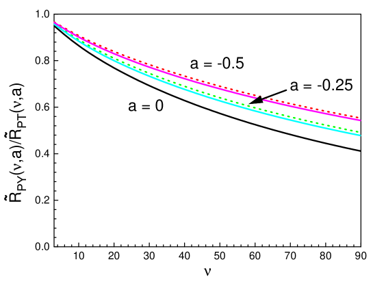
Figure 5: Ratios of moments of angularity cross sections computed from PYTHIA (${\rm\tilde{R}_{PY}}$) to the resummed perturbation theory moments (${\rm\tilde{R}_{PT}}$) for $a=0,\ -0.5,\ -0.5$. the lines for the two latter cases are the predictions of scaling.

Tests of the angularities are only one example of the potential of $\rm e^{+}e^{-}$ event structure to address new questions in the transition from perturbative to nonperturbative dynamics. Most of the event shapes that were used in the analyses of and since the 1990s were invented for the jet physics of the late 1970s. In the intervening time, we have learned how to ask a whole new set of questions, which existing data may be able to answer for us.

V Beyond leading orders and leading powers

While the shape function approach purports to organize the entire set of nonperturbative powers in $\nu/Q$, much of the original discussions eventshapes , including those on angularities Berger03 ; Berger04 were based on NLL resummations. As we have observed above, it is also interesting to search for more complete treatments, which can organize perturbation theory to arbitrary logarithmic orders. Such a treatment can be based on the factorization of soft and collinear dynamics in gauge theories, as already observed in eventshapes . Related results have now been derived in the context of soft-colllinear effective theory Manohar03 , and I hope it will be fruitful to study the relationship between these two methods. [In fact, some steps in this direction were taken at this workshop, and are described in Lee06 .] In closing, I will briefly discuss the factorization-based formalism, and try to give some sense of how it can enable us to establish very general properties in perturbation theory.

V.1 Operators and soft gluon emission

A basic result in factorization analysis is that the coupling of soft gluons to jets is equivalent to their coupling to light-like ordered exponentials, or Wilson lines,

$$\Phi^{(f)}_{\beta}(\lambda,x)={\cal P}\exp\left(-ig\int_{0}^{\lambda}d\lambda^{\prime}\beta\cdot A^{(f)}(\lambda^{\prime}\beta+x)\right)\,,$$ (28)

where the field $A^{(f)}$ is in the matrix representation corresponding to the flavor $f$ of the parton that initiates the jet (quark or antiquark for two-jet events in $\rm e^{+}e^{-}$ annihilation). Once this factorization is carried out, we can define an event shape distribution from the soft gluons to two-jet event shapes $e$,

$${{d\sigma^{({\rm eik})}(e,\{\beta_{i}\})\over de}}=\sum_{N}\ {\delta\left(e-e(N)\right)}\ \langle 0|W^{\dagger}\,{|N\rangle\,\langle N|}\,W\,|0\rangle\,,$$ (29)

where $W$ is a product of Wilson lines for the quark and antiquark,

$$W=T\Bigg{(}\Phi^{(q)}_{\beta_{q}}(\infty,0)\,\Phi^{(\bar{q})}_{\beta_{\bar{q}}}(\infty,0)\Bigg{)}\,.$$ (30)

The perturbative expansion for these matrix elements is equivalent to the eikonal approximation for radiation from a light-like quark pair, illustrated in Fig. 6. The matrix elements above also correspond to the leading operators in the soft-collinear effective theory of Ref. Manohar03 .

In the complete cross section, the soft gluon distribution $d\sigma^{({\rm eik})}/de$, Eq. (29), will appear in convolution with two functions describing the collinear dynamics of the jets. The full cross section therefore factorizes into a simple product in transform space. Nonperturbative corrections of the jet functions should appear as powers in $1/m_{J}^{2}$, corresponding to powers of $\nu/Q^{2}$ in the transform space, which are therefore subleading compared to those from the soft function. A very important point is that the factorization itself becomes better and better for smaller and smaller event shape values, that is, for narrower and narrower jets. Corrections to factorization vanish as powers of $m_{J}/Q$, and therefore decay as powers of $\nu$ in transform space.

Figure 6: Typical (virtual) diagram in the eikonal cross section.

V.2 Eikonal exponentiation for event shapes

The wonderful thing about eikonal cross sections like (29) is that they exponentiate algebraically, in terms of functions whose perturbative properties are simpler than those of the full theory. For shape functions, the results are equivalent to Eq. (LABEL:Eform) but more general.

The relevant functions have been called “webs” webs . The web functions can be written as sums over individual cut diagrams, ${\cal M}^{2}_{N}$. A cut diagram is the union of a diagrammatic contribution to the amplitude for the production of state $N$, with another for the complex conjugate amplitude. The function ${\cal M}^{2}_{N}$ includes all diagrams of this type that cannot be disconnected by cutting only two eikonal lines. Each diagrammatic contribution to ${\cal M}^{2}_{N}$ is associated with a specific, overall modified color factor, $C({\cal M}^{2}_{N})$. The web function at fixed event shape $e$ can then be written formally as

$$E(e)=\sum_{{\rm states}\ N}\ \delta\left(e-e(N)\right)\,\sum_{\cal M}C({\cal M}^{2}_{N})\;{\cal M}^{2}_{N}(e)\,.$$ (31)

Examples of virtual web diagrams are shown in Fig. 7. In this set all have the same modified color factor.

As long as the event shape $e$ can be written as the sum over the contributions of individual final-state particles, the eikonal cross section at fixed total event shape $e$ is a convolution of the form,

$${{d\sigma^{({\rm eik})}(e)\over de}}=\sum_{n=0}^{\infty}\;{1\over n!}\;\prod_{i=1}^{n}\;\int de_{i}\,E(e_{i})\;\delta(e-\sum_{i}e_{i})\,.$$ (32)

It therefore exponentiates under a Laplace transform,

$$\tilde{S}_{e}(\nu,Q)\equiv\int_{0}de\;{\rm e}^{-\nu e}\ {d\sigma^{({\rm eik})}\over de}=\exp\,\left[\int_{0}de^{\prime}\;{\rm e}^{-\nu e^{\prime}}\;E(e^{\prime})\,\right]\,,$$ (33)

where dependence on the upper limit is exponentially suppressed for large $\nu$, corresponding to $e\to 0$.

Figure 7: Examples of virtual web diagrams. The webs are irreducible under cuts of two eikonal lines. All of these webs have the same color factor, which in the full theory is the color factor corresponding to the web with the three-gluon vertex.

For light-like eikonal lines, the web functions themselves are boost and renormalization group invariant. To get a sense of how these properties can be used, consider a trivial event shape, in which the radiated energy is fixed. By itself, such a cross section would have collinear singularitites, but these can be systematically subtracted. Indeed this is just what happens in a Drell-Yan cross section when the eikonal lines are incoming, or for a two-particle correlation cs81 when the eikonal lines are outgoing. In either case, the eikonal annihilation cross section takes the form joint

$$\ln\tilde{S}_{\rm incl}(\nu,Q) = \sum_{{\rm states}\ N}\ \sum_{\cal M}C({\cal M}^{2}_{N})\;{\cal M}^{2}_{N}(E_{N}/Q)\ e^{-\nu E_{N}/Q}$$ (34)

$$= \int_{0}^{Q^{2}}\frac{\rho(\alpha_{s}(u,\varepsilon))}{u^{2}}\;\left[K_{0}\left(\frac{2\nu u}{Q}\right)+\ln\frac{u}{Q}\right]+2\ln\bar{\nu}\int_{0}^{Q^{2}}\frac{du^{2}}{u^{2}}A(\alpha_{s}(u,\varepsilon))\,,$$

where boost and renormalization group invariance implies that the spectral function $\rho(\alpha_{s})$ can be written as a function of the running $\alpha_{s}$ only. Here $\bar{\nu}\equiv\nu e^{-\gamma_{E}}$ with $\gamma_{E}$ the Euler constant, and the integrals are defined by dimensional regularization in $D=4-2\varepsilon$ dimensions.

The final term in Eq. (34) represents the collinear subtractions, and for such inclusive cross sections, the relevant factorization theorems actually require a generalization of the “MC-scheme” mentioned above, relating the spectral function to the anomalous dimension $A(\alpha_{s})$ to all orders in perturbation theory, with a correction that begins at next-to-next to leading logarithm,

$$\rho(\alpha_{s}(u,\varepsilon))=2A(\alpha_{s}(u,\varepsilon))+\frac{\partial D(\alpha_{s},\varepsilon)}{\partial\ln\mu^{2}}\,.$$ (35)

In four dimensions, this correction, $D(\alpha_{s},0)$ is the all-orders generalization of the NNLL “D-term”, long known in the resummed Drell-Yan cross section Dterms .

Equation (34) is a true internally resummed expression. The very specific form of the term in square brackets, involving the Bessel function, follows from boost invariance along the two-jet axis, and is accurate up to corrections that decay exponenetially in $\nu$. Expanded in powers of $\nu u/Q$, this predicts the form of power corrections (even powers only), by the standard reasoning above.

We also learn from (34) that at NNLL the MC scheme, and presumably its dispersive property, inherits what appear to be process-dependent corrections. The presence of such corrections, however, should allow us to test ideas like the freezing of the coupling as we learn to apply these methods to more general classes of observables, including event shapes.

VI Conclusion: Looking Toward the Far Infrared

The phenomenology of power corrections, especially in event shapes, is one of the success stories of the past generation of high energy colliders. Moving beyond the current stage of phenomenology, however, to a better understanding of the physics will require both new ideas and accessibility for data sets that can be used to test them.

Looking at just the few topics touched on above, it is clear that a fuller phenomenology waits on systematic insights into formally-nonleading corrections that appear at the level of powers of $\nu/Q^{2}$ in many event shapes. Such corrections are closely connected to hadronization within jets, and hence to parton-hadron duality duality , already familiar from deep-inelastic scattering in the narrow-jet, that is $x\to 1$, limit. This general question may also be related to the role of the nonleading power corrections in the $a<1$ angularities mentioned below Eq. (26).

A central issue still in the background is the role of quarks. Most of the analysis of resummation and power corrections is driven by gluons, but eventually, it’s primarily quarks that characterize the hadrons that we observe. Finally, as hinted at above, the study of power corrections should eventually overlap with event generator concepts like clusters and string breaking. It is my hope that this workshop will be a stimulus for addressing these problems, and the many others that I’ve surely missed.

- (1) C.N. Yang, in High Energy Collisions, Third International Conference, Stony Brook, New York, Sept. 5 and 6, 1969, ed. C.N. Yang, J.A. Cole, M. Good, R. Hwa and J. Lee-Franzini (Gordon and Breach, New York, 1969).
- (2) A. H. Mueller, Nucl. Phys. B 250, 327 (1985); Phys. Lett. B 308, 355 (1993).
- (3) G. ’t Hooft, lectures Int. School of Subnuclear Physics, Erice, Sicily, Jul 23 - Aug 10, 1977; in Erice Subnucl.1977, 943, and Under the spell of the gauge principle, (World Scientific, Singapore, 2005) ed. G. ’t Hooft, p. 547.
- (4) M. A. Shifman, A. I. Vainshtein and V. I. Zakharov, Nucl. Phys. B 147, 385 (1979).
- (5) G. Sterman, Phys. Rev. D 17, 2773 (1978); and An Introduction to quantum field theory (Cambridge Univ. Press, 1993) Chap. 13.
- (6) G. Sterman, at International Conference on Theoretical Physics (TH 2002), Paris, France, 22-26 Jul 2002, in Int. J. Mod. Phys. A18, 4329 (2003) and Annales Henri Poincare 4 S259 (2003) hep-ph/0301243.
- (7) A. Dhar and V. Gupta, Phys. Rev. D 29, 2822 (1984); G. Grunberg, Phys. Rev. D 29, 2315 (1984); C. J. Maxwell and A. Mirjalili, Nucl. Phys. B 577, 209 (2000) [arXiv:hep-ph/0002204]; J. Abdallah et al. [DELPHI Collaboration], Eur. Phys. J. C 29, 285 (2003) [arXiv:hep-ex/0307048],
- (8) L. N. Lipatov, Sov. Phys. JETP 45, 216 (1977) [Zh. Eksp. Teor. Fiz. 72, 411 (1977)]; E. Brezin, J. C. Le Guillou and J. Zinn-Justin, Phys. Rev. D 15, 1544 (1977)
- (9) A. I. Vainshtein and V. I. Zakharov, Phys. Rev. Lett. 73, 1207 (1994) [Erratum-ibid. 75, 3588 (1995)] [arXiv:hep-ph/9404248]; G. Altarelli, P. Nason and G. Ridolfi, Z. Phys. C 68, 257 (1995) [arXiv:hep-ph/9501240]; M. Beneke, V. M. Braun and N. Kivel, Phys. Lett. B 404, 315 (1997) [arXiv:hep-ph/9703389]; R. Akhoury and V. I. Zakharov, Nucl. Phys. Proc. Suppl. 64, 350 (1998) [arXiv:hep-ph/9710257].
- (10) M. Beneke and V.M. Braun, in the Boris Ioffe Festschrift At the frontier of particle physics / handbook of QCD, ed. M. Shifman (World Scientific, Singapore, 2001) [ArXiv:hep-ph/0010208].
- (11) M. Dasgupta and G. P. Salam, J. Phys. G 30, R143 (2004) [arXiv:hep-ph/0312283].
- (12) D. Appell, G. Sterman and P. B. Mackenzie, in Proceedings of the Storrs Meeting, ed. K. Haller et al., (World Scientific, Singapore, 1989) p. 567; H. Contopanagos and G. Sterman, Nucl. Phys. B 419, 77 (1994) [arXiv:hep-ph/9310313]; A. V. Manohar and M. B. Wise, Phys. Lett. B 344, 407 (1995) [arXiv:hep-ph/9406392]; G. P. Korchemsky and G. Sterman, Nucl. Phys. B 437, 415 (1995) [arXiv:hep-ph/9411211]; M. Beneke and V. M. Braun, Nucl. Phys. B 454, 253 (1995) [arXiv:hep-ph/9506452]; R. Akhoury and V. I. Zakharov, Phys. Lett. B 357, 646 (1995) [arXiv:hep-ph/9504248]; Nucl. Phys. B 465, 295 (1996) [arXiv:hep-ph/9507253]; Phys. Rev. Lett. 76, 2238 (1996) [arXiv:hep-ph/9512433]; M. Dasgupta and B. R. Webber, Phys. Lett. B 382, 273 (1996) [arXiv:hep-ph/9604388] M. Dasgupta and B. R. Webber, Nucl. Phys. B 484, 247 (1997) [arXiv:hep-ph/9608394]; M. Beneke, V. M. Braun and L. Magnea, Nucl. Phys. B 497, 297 (1997) [arXiv:hep-ph/9701309].
- (13) B. R. Webber, Phys. Lett. B 339, 148 (1994) [arXiv:hep-ph/9408222].
- (14) P. Nason and M. H. Seymour, Nucl. Phys. B 454, 291 (1995) [arXiv:hep-ph/9506317].
- (15) R. Basu, Phys. Rev. D 29, 2642 (1984); Z. Trocsanyi, JHEP 0001, 014 (2000) [arXiv:hep-ph/9911353]; S. Banerjee and R. Basu, Pramana 59, 457 (2002) [arXiv:hep-ph/0006008].
- (16) I. I. Y. Bigi, M. A. Shifman, N. G. Uraltsev and A. I. Vainshtein, Phys. Rev. D 50, 2234 (1994) [arXiv:hep-ph/9402360].
- (17) E. Gardi, Nucl. Phys. B 622, 365 (2002) [arXiv:hep-ph/0108222].
- (18) C. F. Berger and L. Magnea, Phys. Rev. D 70, 094010 (2004) [arXiv:hep-ph/0407024].
- (19) Y. L. Dokshitzer, G. Marchesini and B. R. Webber, Nucl. Phys. B 469, 93 (1996) [arXiv:hep-ph/9512336].
- (20) S. J. Brodsky, E. Gardi, G. Grunberg and J. Rathsman, Phys. Rev. D 63, 094017 (2001) [arXiv:hep-ph/0002065]; Y. L. Dokshitzer and D. E. Kharzeev, Ann. Rev. Nucl. Part. Sci. 54, 487 (2004) [arXiv:hep-ph/0404216].
- (21) C. L. Basham, L. S. Brown, S. D. Ellis and S. T. Love, Phys. Rev. D 17, 2298 (1978); N. A. Sveshnikov and F. V. Tkachov, Phys. Lett. B 382, 403 (1996) [arXiv:hep-ph/9512370]; F. V. Tkachov, Int. J. Mod. Phys. A 12, 5411 (1997) [arXiv:hep-ph/9601308]; G. P. Korchemsky, G. Oderda and G. Sterman, in 5th International Workshop on Deep Inelastic Scattering and QCD (DIS 97), AIP Conference Proceedings 407, ed. J. Repond, D. Krakauer (American Institute of Physics, Woodbury, NY 1978), p. 988 [arXiv:hep-ph/9708346]; C. F. Berger et al., in Proc. of the APS/DPF/DPB Summer Study on the Future of Particle Physics (Snowmass 2001) ed. N. Graf, eConf C010630, P512 (2001) [arXiv:hep-ph/0202207].
- (22) G. Sterman, Phys. Rev. D 19, 3135 (1979).
- (23) Y. L. Dokshitzer, A. Lucenti, G. Marchesini and G. P. Salam, Nucl. Phys. B 511, 396 (1998) [Erratum-ibid. B 593, 729 (2001)] [arXiv:hep-ph/9707532]; Y. L. Dokshitzer, A. Lucenti, G. Marchesini and G. P. Salam, JHEP 9805, 003 (1998) [arXiv:hep-ph/9802381].
- (24) A. Banfi, Y. L. Dokshitzer, G. Marchesini and G. Zanderighi, JHEP 0105, 040 (2001) [arXiv:hep-ph/0104162]; A. Banfi, G. Marchesini, G. Smye and G. Zanderighi, JHEP 0111, 066 (2001) [arXiv:hep-ph/0111157].
- (25) J. C. Collins and D. E. Soper, Nucl. Phys. B 193, 381 (1981) [Erratum-ibid. B 213, 545 (1983)].
- (26) Y.L. Dokshitzer, D.I. D’Yakonov and S.I. Troyan, Phys. Lett. 79B (1978) 269; G. Parisi and R. Petronzio, Nucl. Phys. B 154 (1979) 427; G. Altarelli, R.K. Ellis, M. Greco and G. Martinelli, Nucl. Phys. B 246 (1984) 12; J.C. Collins and D.E. Soper, Nucl. Phys. B 193 (1981) 381; E: ibid B 213 (1983) 545; Nucl. Phys. B 197 (1982) 446; J.C. Collins, D.E. Soper and G. Sterman, Nucl. Phys. B 250 (1985) 199; C.T.H. Davies and W.J. Stirling, Nucl. Phys. B 244 (1984) 337; C.T.H. Davies, W.J. Stirling and B.R. Webber, Nucl. Phys. B 256 (1985) 413; P.B. Arnold and R.P. Kauffman, Nucl. Phys. B 349 (1991) 381; G.A. Ladinsky and C.-P. Yuan, Phys. Rev. D 50 (1994) 4239, [hep-ph/9311341]; F. Landry, R. Brock, G. Ladinsky and C.-P. Yuan, Phys. Rev. D 63 (2001) 013004, [hep-ph/9905391]; C. Balazs and C.P. Yuan, Phys. Rev. D 56 (1997) 5558, [hep-ph/9704258]; J.-w. Qiu and X.-f. Zhang, Phys. Rev. Lett. 86 (2001) 2724, [hep-ph/0012058]; Phys. Rev. D 63 (2001) 114011, [hep-ph/0012348]; E. L. Berger and J.-w. Qiu, Phys. Rev. D 67, 034026 (2003) [arXiv:hep-ph/0210135]; H.-N. Li, Phys. Lett. B 454 (1999) 328, [hep-ph/9812363]. A. Kulesza, G. Sterman and W. Vogelsang, Phys. Rev. D 66 (2002) 014011, [hep-ph/0202251].
- (27) C. F. Berger, T. Kùcs and G. Sterman, Phys. Rev. D 68, 014012 (2003) [arXiv:hep-ph/0303051].
- (28) A. Banfi, G. P. Salam and G. Zanderighi, JHEP 0503, 073 (2005) [arXiv:hep-ph/0407286].
- (29) C. F. Berger and G. Sterman, JHEP 0309, 058 (2003) [arXiv:hep-ph/0307394].
- (30) S. Catani, G. Turnock, B. R. Webber, L. Trentadue, Phys. Lett. B 263, 491 (1991); S. Catani, L. Trentadue, G. Turnock, B. R. Webber, Nucl. Phys. B 407, 3 (1993).
- (31) G. P. Korchemsky and G. Sterman, arXiv:hep-ph/9505391; Y. L. Dokshitzer and B. R. Webber, Phys. Lett. B 404, 321 (1997) [arXiv:hep-ph/9704298].
- (32) G. P. Korchemsky, Shape functions and power corrections to the event shapes, in Minneapolis 1998, Continuous advances in QCD, 179 (1998) [arXiv:hep-ph/9806537]; G. P. Korchemsky and G. Sterman, Nucl. Phys. B 555, 335 (1999) [arXiv:hep-ph/9902341].
- (33) G. P. Korchemsky and S. Tafat, JHEP 0010, 010 (2000) [arXiv:hep-ph/0007005]; E. Gardi and J. Rathsman, Nucl. Phys. B 609, 123 (2001) [arXiv:hep-ph/0103217]; E. Gardi and J. Rathsman, Nucl. Phys. B 638, 243 (2002) [arXiv:hep-ph/0201019]; E. Gardi and L. Magnea, JHEP 0308, 030 (2003) [arXiv:hep-ph/0306094.
- (34) T. Chandramohan and L. Clavelli, Nucl. Phys. B 184, 365 (1981).
- (35) A. V. Belitsky, G. P. Korchemsky and G. Sterman, Phys. Lett. B 515, 297 (2001) [arXiv:hep-ph/0106308].
- (36) C. W. Bauer, A. V. Manohar and M. B. Wise, Phys. Rev. Lett. 91, 122001 (2003) [arXiv:hep-ph/0212255]; C. W. Bauer, C. Lee, A. V. Manohar and M. B. Wise, Phys. Rev. D 70, 034014 (2004) [arXiv:hep-ph/0309278].
- (37) C. Lee and G. Sterman, arXiv:hep-ph/0603066.
- (38) G. Sterman, in AIP Conference Proceedings Tallahassee, Perturbative Quantum Chromodynamics, eds. D. W. Duke, J. F. Owens, New York, 1981, p. 22; J. G. Gatheral, Phys. Lett. B 133, 90 (1983); J. Frenkel and J. C. Taylor, Nucl. Phys. B 246, 231 (1984); G. P. Korchemsky and A. V. Radyushkin, Phys. Lett. B 171, 459 (1986); C. F. Berger, Phys. Rev. D 66, 116002 (2002) [ArXiv:hep-ph/0209107].
- (39) E. Laenen, G. Sterman and W. Vogelsang, Phys. Rev. D 63, 114018 (2001) [arXiv:hep-ph/0010080].
- (40) G. Sterman, Nucl. Phys. B 281, 310 (1987); S. Catani and L. Trentadue, Nucl. Phys. B 327, 323 (1989); Nucl. Phys. B 353, 183 (1991); A. Vogt, Phys. Lett. B 497, 228 (2001) [arXiv:hep-ph/0010146].
- (41) W. Melnitchouk, R. Ent and C. Keppel, Phys. Rept. 406, 127 (2005) [arXiv:hep-ph/0501217].