CERN-PH-TH/2006-097

On the electroweak symmetry breaking
in the Littlest Higgs model
Antonio Dobado, Lourdes Tabares
Departamento de Física Teórica I,

Universidad Complutense de Madrid, E-28040 Madrid, Spain

and

Siannah Peñaranda
CERN TH Division, Department of Physics, CH-1211 Geneva 23, Switzerland

and IFIC - Instituto de Física Corpuscular, CSIC - Universitat de València,

Apartado de Correos 22085, E-46071 Valencia, Spain

ABSTRACT

In the $SU(5)/SO(5)$ little Higgs models radiative corrections give rise to the $SU(2)_{L}\times U(1)_{Y}$ symmetry breaking. In this work we start a program for a detailed determination of the relevant terms of the Higgs effective potential by computing the contribution of the $b$, $t$ and $T$ quarks at the one-loop level, as an starting point for higher-loops computation. In spite of the fact that some two-loop level contributions are well known to be important, we use our preliminary one-loop result to illustrate that, by demanding the effective potential to reproduce exactly the Standard Model Higgs potential, and in particular the relation $m_{H}^{2}=2\lambda v^{2}=2\mu^{2}$, it will be possible to set new constraints on the parameter space of the Littlest Higgs model when the computation of all the relevant contributions to the Higgs effective potential is completed.

1 Introduction

In the last years a lot of work has been devoted to the so-called little Higgs models (see [1] and [2] for recent reviews). These models use an old suggestion by Georgi and Pais [3] in which the Higgs is assumed to be a (pseudo) Goldstone boson associated to some global spontaneous symmetry breaking [4]. For instance, in the case of the paradigmatic Littlest Higgs (LH) [5], a $SU(5)$ to $SO(5)$ breaking is assumed to happen at some scale $f$. The Higgs field is just one of the corresponding $14$ Goldstone bosons and therefore it is, in principle, massless. The $SU(5)$ subgroup $(SU(2)\times U(1))_{1}\times(SU(2)\times U(1))_{2}$ is gauged so that the axial $(SU(2)\times U(1))_{1-2}$ is spontaneously broken, the corresponding gauge bosons being typically heavy ($W^{\prime a}$ and $B^{\prime}$). The diagonal $(SU(2)\times U(1))_{1+2}=SU(2)_{L}\times U(1)_{Y}$ remains unbroken and corresponds to the electroweak SM group. However, radiative corrections coming from the fermionic sector of the model, mainly the third quark generation and an additional vector-like quark $T,$ give rise to an effective potential that produces a further spontaneous symmetry breaking of the SM $SU(2)_{L}\times U(1)_{Y}$ down to $U(1)_{\rm{em}}$. In this way some of the Goldstone bosons acquire masses quadratic in the cut-off $\Lambda$, which is expected to be of the order of $4\pi f$ [6], but the SM model Higgs gets a mass that grows only as the logarithm of $\Lambda$ at the one-loop level. This is the explanation in this setting of why the Higgs is expected to be relatively light ($115$ GeV $<m_{H}<200$ GeV). The rest of the Goldstone bosons gives masses to the different gauge bosons through the Higgs mechanism in the $SU(5)$ to $SO(5)$ or in the SM breaking. Thus, the LH model explains in a natural and elegant way the expected low value of the Higgs boson mass. In addition this model provides a very rich phenomenology, which could be probed in the next-generation colliders such as the LHC [7, 8]. Since the original proposal of the LH, many other little Higgs versions have appeared [9]. Some of these models try to improve the consistency and reduce the need for fine-tuning in this kind of models (see [10] for details). Specially interesting from the phenomenological point of view is the LH version in which the $SU(5)$ gauged subgroup is just $SU(2)_{1}\times SU(2)_{2}\times U(1)$. In this case, after the first spontaneous broken symmetry, we have only three massive gauge bosons associated to the $SU(2)_{1-2}$ group, $W^{\prime a}$, and four massless gauge bosons, i.e. the SM gauge bosons [8].

Nevertheless, it is clear that any viable little Higgs model has to fulfil the basic requirement of reproducing the SM model at low energies. This implies, in particular, not only to have the proper low energy degrees of freedom, but also to reproduce the SM model action as the low energy effective action of the LH model, whenever one be near the physical minimum. In this work we compute the contribution of the $t,b$ and $T$ quarks to the effective potential for the SM Higgs doublet $H=(H^{0},H^{+})$, which gives rise to the electroweak symmetry breaking in the LH model. The first terms of this potential are found to have the standard form:

$$V_{\rm{eff}}=-\mu^{2}HH^{{\dagger}}+\lambda(HH^{{\dagger}})^{2}\,,$$ (1.1)

with positive $\mu^{2}$ and $\lambda$. Other relevant contributions coming from gauge bosons, scalars and other higher loops are expected to go in the opposite direction, but they are also supposed to have a smaller absolute value so that they do not change the $\mu^{2}$ and $\lambda$ signs. The $\mu^{2}$ sign and value are well known [5, 8], and effectively they are the right ones to produce the electroweak symmetry breaking, giving a Higgs mass $m_{H}^{2}=2\mu^{2}$. However, the full expression for $\lambda$ has not been analyzed in detail. Several relations for the threshold corrections to this parameter in the presence of a $10$ TeV cut-off, depending of the UV-completion of the theory, has been reported before (see, for example [11]). The radiative corrections to $\lambda$, at the one-loop level, have not been computed so far.

The computation of the $\lambda$ parameter is important for several reasons. First, it must be positive, for the low energy effective action to make sense (otherwise the theory would not have any vacuum). In addition, from the effective potential above, one gets the simple formula $m^{2}_{H}=2\lambda v^{2}$ or, equivalently, $\mu^{2}=\lambda v^{2}$, where $v$ is the SM vacuum expectation value ($H=(0,v)/\sqrt{2}$), which is set by experiment (for instance from the muon lifetime) to be $v\simeq 245$ GeV. By computing the effective action by the Higgs doublet in the context of the LH model, taking into account the $t,b$ and $T$ quarks only, i.e. the modes responsible for the electroweak symmetry breaking, it is possible to obtain $\mu^{2}$ and $\lambda$ in terms of the $\lambda_{T},f$ and $\Lambda$ parameters of the LH model, where $\lambda_{T}$ is the $T$ Yukawa coupling, $f$ is the scale of the $SU(5)/SO(5)$ symmetry breaking, and $\Lambda$ is the ultraviolet cut-off (in fact $\lambda$ has also a small dependence on an infrared cut-off $m\sim v$). In other words, we can find the functions:

$$\mu^{2}=\mu^{2}\,(\lambda_{T},f,\Lambda)\,,$$

$$\lambda=\lambda\,(\lambda_{T},f,\Lambda)\,.$$ (1.2)

As is well known, $\mu$ depends on the logarithm of $\Lambda$ at one-loop level, but $\lambda$ has also a much stronger quadratic dependence on this cut-off. Moreover, according to the previous discussion, the consistency of the low energy theory sets the following highly non-trivial constraint on the LH model parameters:

$$\mu^{2}(\lambda_{T},f,\Lambda)=\lambda(\lambda_{T},f,\Lambda)v^{2}+...\,,$$ (1.3)

where the periods include corrections coming from gauge bosons, scalars and other higher order loops.

In this work we compute the contribution to these functions coming from the $t,b$ and $T$ quarks present in the LH model at the one-loop level which are the relevant ones for having symmetry breaking. Then we use the result to illustrate the kind of bounds and restrictions that must be set on the LH model fermion parameters in order to obtain the SM potential from the effective Higgs potential which should also include gauge, scalar and other higher loop contributions [18]. This analysis is crucial if one assumes that the new physics decouples from the low energy scale.

The outline of the paper is as follows: In Section 2 we review briefly the LH model and set the notation we are going to use. In Section 3 we compute the effective action for a constant SM Higgs doublet, i.e. the effective potential, by using standard techniques (see for example [12]), and we obtain the $\mu=\mu(\lambda_{T},f,\Lambda)$ and $\lambda=\lambda(\lambda_{T},f,\Lambda)$ functions. Section 4 is devoted to the study of the above-mentioned constraints that our computation sets on the LH model parameter space and, finally, in Section 5 we summarize our main results and present some conclusions and remarks.

2 The model

The LH model is based on the assumption that there is a physical system with a global $G=SU(5)$ symmetry, which is spontaneously broken to a $H=SO(5)$ symmetry at a high scale $\Lambda$ through a vacuum expectation value of order $f$. Thus the spectrum of the theory will contain in principle $14$ Goldstone bosons including the SM complex doublet $H=(H^{0},H^{+})$. In addition, the $SU(5)$ subgroup $(SU(2)\times U(1))_{1}\times(SU(2)\times U(1))_{2}$ is gauged, its diagonal subgroup $(SU(2)\times U(1))_{1+2}$ being the SM electroweak group $SU(2)_{L}\times U(1)_{Y}$. This group remains unbroken after the $SU(5)$ breaking to $SO(5)$ and consequently the electroweak gauge bosons $W_{\mu}^{a}$ and $B_{\mu}$ are massless at this level. However, the $(SU(2)\times U(1))_{1-2}$ group becomes spontaneously broken and the corresponding gauge bosons $W_{\mu}^{{}^{\prime}a}$ and $B^{\prime}_{\mu}$ get masses of order $f$ through the Higgs mechanism. Each of these two gauge groups must commute with a different subgroup $SU(3)$ that acts non-linearly on the Higgs, i.e. when both weak gauge interactions are included, the Higgs is a pseudo-Goldstone boson whose mass is protected by the underlying symmetry but, conversely, if just one of these interactions is considered, the $SU(3)$ symmetry is recovered [5].

With the global $SU(5)$ symmetry breaking into its subgroup $SO(5)$, we have $14$ Goldstone bosons, which transform under the electroweak group as a real singlet, a real triplet, a complex doublet and a complex triplet. The real singlet and the real triplet become the longitudinal part of the $B^{\prime}_{\mu}$ and $W_{\mu}^{{}^{\prime}a}$ bosons through the Higgs mechanism, and the last two Goldstone boson multiplets can be interpreted as the SM Higgs doublet and an additional complex triplet, i.e. we still have $10$ massless Goldstone bosons. These particles will get radiative masses after the introduction of appropriate gauge and Yukawa couplings to the third-generation $b$ and $t$ quarks and an additional vector-like quark $T$, the Yukawa contributions being responsible to give the expected sign to the Higgs doublet mass. Then, the magic of the model produces a Higgs mass, which is quadratically divergence-free at the one-loop level. In this way we obtain a light Higgs in a natural way, thanks to the pseudo-Goldstone boson nature of this field. The complex triplet is not protected in the same way and quark radiative corrections make it typically much more massive, thus evading the experimental constraints.

According to the previous discussion, the low energy dynamics of the LH model can be described by a $(SU(2)\times U(1))_{1}\times(SU(2)\times U(1))_{2}$ gauged non-linear sigma model based on the coset $K=G/H=SU(5)/SO(5)$ (see for instance [12]). The Goldstone boson fields can be arranged in a $5\times 5$ matrix $\Sigma$ given by:

$$\Sigma=e^{2i\Pi/f}\Sigma_{0},$$ (2.4)

where:

$$\Sigma_{0}=\left(\begin{array}[]{ccc}0&0&\textbf{1}\\ 0&1&0\\ \textbf{1}&0&0\\ \end{array}\right)$$ (2.5)

has the proper $SU(5)$ symmetry breaking structure, 1 being the $2\times 2$ unit matrix, and

$$\Pi=\left(\begin{array}[]{ccc}\xi&\frac{-i}{\sqrt{2}}H^{{\dagger}}&\phi^{{\dagger}}\\ \frac{i}{\sqrt{2}}H&0&\frac{-i}{\sqrt{2}}H^{*}\\ \phi&\frac{i}{\sqrt{2}}H^{T}&\xi^{T}\\ \end{array}\right)+\frac{1}{\sqrt{20}}\,\eta\,{\mbox{diag }}(1,1,-4,1,1)$$ (2.6)

is the Goldstone bosons matrix, with $H=(H^{0},H^{+})$ the SM Higgs doublet, $\eta$ being the real scalar, and $\xi$ and $\phi$ encoding the real triplet and the complex triplet respectively:

$$\xi=\left(\begin{array}[]{cc}\frac{1}{2}\xi^{0}&\frac{1}{\sqrt{2}}\xi^{+}\\ \frac{1}{\sqrt{2}}\xi^{-}&-\frac{1}{2}\xi^{0}\end{array}\right)~{}~{}~{}~{}~{}~{}~{}~{}~{}~{}~{}{\mbox{ and }}~{}~{}~{}~{}~{}~{}~{}~{}~{}~{}~{}~{}\phi=\left(\begin{array}[]{cc}\phi^{0}&\frac{1}{\sqrt{2}}\phi^{+}\\ \frac{1}{\sqrt{2}}\phi^{+}&\frac{1}{\sqrt{2}}\phi^{++}\end{array}\right)\,.$$ (2.7)

The Lagrangian of the gauged non-linear sigma model is given by:

$${\cal L}_{0}=\frac{f^{2}}{8}\mbox{tr}D_{\mu}\Sigma(D^{\mu}\Sigma)^{\dagger}\,,$$ (2.8)

where the covariant derivative is defined as [5]:

$$D_{\mu}\Sigma=\partial_{\mu}\Sigma-i\sum_{j=1}^{2}g_{j}W^{a}_{j}(Q_{j}^{a}\Sigma+\Sigma Q_{j}^{aT})-i\sum_{j=1}^{2}g^{\prime}_{j}B_{j}(Y_{j}\Sigma+\Sigma Y_{j}^{T})\,,$$ (2.9)

where $g_{j}$ and $g^{\prime}_{j}$ are the gauge couplings, $Q_{1ij}^{a}=\sigma_{ij}^{a}/2$ for $i,j=1,2$, $Q_{2ij}^{a}=\sigma_{ij}^{a*}/2$ for $i,j=4,5$, and zero otherwise, $Y_{1}=$ diag$(-3,-3,2,2,2)/10$ and $Y_{2}=$ diag$(-2,-2,-2,3,3)/10$. By diagonalizing the gauge boson mass matrix contained in this Lagrangian one gets the massless $W$ and $B$ SM bosons and the massive $W^{\prime}$ and $B^{\prime}$ gauge bosons mentioned above as:

$$W^{a} = c_{\psi}W_{1}^{a}+s_{\psi}W_{2}^{a}$$

$$W^{{}^{\prime}a} = s_{\psi}W_{1}^{a}-c_{\psi}W_{2}^{a}\,,$$ (2.10)

where

$$s_{\psi} = \sin\psi=\frac{g_{1}}{\sqrt{g_{1}^{2}+g_{2}^{2}}}$$

$$c_{\psi} = \cos\psi=\frac{g_{2}}{\sqrt{g_{1}^{2}+g_{2}^{2}}}$$ (2.11)

with $M_{W}=0$ and $M_{W^{\prime}}=f\sqrt{g_{1}^{2}+g_{2}^{2}}/2$. In a similar way we have

$$B = c^{\prime}_{\psi}B_{1}+s^{\prime}_{\psi}B_{2}$$ (2.12)

$$B^{\prime} = s^{\prime}_{\psi}B_{1}-c^{\prime}_{\psi}B_{2}\,,$$

where

$$s^{\prime}_{\psi} = \sin\psi^{\prime}=\frac{g^{\prime}_{1}}{\sqrt{{g^{\prime}}_{1}^{\,2}+{g^{\prime}}_{2}^{\,2}}}$$ (2.13)

$$c^{\prime}_{\psi} = \cos\psi^{\prime}=\frac{{g^{\prime}}_{2}}{\sqrt{{g^{\prime}}_{1}^{\,2}+{g^{\prime}}_{2}^{\,2}}}\,,$$

where $M_{B}=0$ and $M_{B^{\prime}}=f\sqrt{g_{1}^{{}^{\prime}2}+g_{2}^{{}^{\prime}2}}/\sqrt{20}$.

A modified version of the LH models, such that the gauge subgroup of $SU(5)$ is $[SU(2)\times SU(2)\times U(1)_{Y}]$ rather than $[SU(2)\times U(1)_{Y}]^{2}$, has also been introduced [8]. In this case, the covariant derivative is defined as:

$$D_{\mu}\Sigma=\partial_{\mu}\Sigma-i\sum_{j=1}^{2}g_{j}W^{a}_{j}(Q_{j}^{a}\Sigma+\Sigma Q_{j}^{aT})-ig^{\prime}B(Y\Sigma+\Sigma Y^{T})\,,$$ (2.14)

where the generators $Q_{j}^{a}$ are the same as in the previous case, and $Y=\frac{1}{2}$diag$(-1,-1,0,1,1)$. The field content of the matrix $\Pi$ in $\Sigma$ is the same as in the LH model but there is no $B^{{}^{\prime}}$ now. This model will be considered in Section 4 when some phenomenological consequences of considering the gauge sector are discussed.

Then, at the tree level, the $SU(2)_{L}\times U(1)_{Y}$ SM gauge group remains unbroken. The spontaneous symmetry breaking of this group is produced in this model radiatively mainly by the quark loops from the third generation, which will be initially denoted by $u$ and $t$ and the additional vector-like quark denoted by $U.$ The interactions between these fermions and the Goldstone bosons are given by the Yukawa Lagrangian:

$$\textit{L}_{\rm{Yuk}}=-\frac{\lambda_{1}}{2}f\,\overline{u}_{R}\,\epsilon_{mn}\,\epsilon_{ijk}\,\Sigma_{im}\,\Sigma_{jn}\,\chi_{Lk}-\lambda_{2}\,f\,{\overline{U}}_{R}\,U_{L}+\mbox{h.c.},$$ (2.15)

where $m,n=4,5$, $i,j=1,2,3$, and

$$\overline{u}_{R} = c\,\overline{t}_{R}+s\,{\overline{T}}_{R}\,,$$

$${\overline{U}}_{R} = -s\,\overline{t}_{R}+c\,{\overline{T}}_{R},$$ (2.16)

with:

$$c = \cos\theta=\frac{\lambda_{2}}{\sqrt{\lambda_{1}^{2}+\lambda_{2}^{2}}},$$

$$s = \sin\theta=\frac{\lambda_{1}}{\sqrt{\lambda_{1}^{2}+\lambda_{2}^{2}}}\,,$$ (2.17)

and

$$\chi_{L}=\left(\begin{array}[]{c}u\\ b\\ U\\ \end{array}\right)_{L}=\left(\begin{array}[]{c}t\\ b\\ T\\ \end{array}\right)_{L}.$$ (2.18)

Here $t\,,b$, $T$ are the mass eigenvectors coming from the mass matrix included in the Yukawa Lagrangian with eigenvalues: $m_{t}=m_{b}=0$ and $m_{T}=f\sqrt{\lambda_{1}^{2}+\lambda_{2}^{2}}$. Thus the quark $t$ is massless and it acquires mass only when the electroweak symmetry is broken, contrary to the quark $T$, which is massive already at this level.

Then, the Yukawa Lagrangian can be written as:

$$\textit{L}_{\rm{Yuk}}=\overline{\chi}_{R}\,\hat{I}_{3x3}\,\chi_{L}+\mbox{h.c.}\,,$$ (2.19)

$\hat{I}_{3x3}$ being the interaction matrix defined below, and

$$\chi_{R}=\left(\begin{array}[]{c}t\\ b\\ T\\ \end{array}\right)_{R}\,.$$

Since we are interested in the computation of the fermion contribution to the SM Higgs effective potential, we set $\xi=\phi=\eta=0$ and thus, the interaction matrix $\hat{I}$ is given by:

$$\hat{I}=\left(\begin{array}[]{ccc}-\sqrt{2}\lambda_{1}cH^{0}\Theta&-\sqrt{2}\lambda_{1}cH^{+}\Theta&\lambda_{1}c\frac{HH^{{\dagger}}}{f}\Theta^{{}^{\prime}}\\ 0&0&0\\ -\sqrt{2}\lambda_{1}sH^{0}\Theta&-\sqrt{2}\lambda_{1}sH^{+}\Theta&\lambda_{1}s\frac{HH^{{\dagger}}}{f}\Theta^{{}^{\prime}}\end{array}\right),$$ (2.23)

where $\Theta$ and $\Theta^{{}^{\prime}}$ are functions on $HH^{\dagger}/f^{2}$ whose expansion starts as:

$$\Theta\left(\frac{HH^{{\dagger}}}{f^{2}}\right)=1-\frac{2HH^{{\dagger}}}{3f^{2}}+...$$ (2.24)

$$\Theta^{\prime}\left(\frac{HH^{{\dagger}}}{f^{2}}\right)=1-\frac{HH^{{\dagger}}}{3f^{2}}+...$$

Therefore the complete Lagrangian for the quarks is:

$$\textit{L}_{\chi} = \textit{L}_{0}+\textit{L}_{\rm{Yuk}}=\overline{\chi}_{R}(i{\partial\mkern-9.0mu/}-M+\hat{I})\chi_{L}+\mbox{h.c.}$$ (2.25)

with $M=$diag$(0,0,m_{T})$.

In the LH model the electroweak symmetry breaking is produced mainly by the three quarks included in the above Lagrangian, whilst the gauge bosons and the complex triplet tend to restore the symmetry. In the following we will consider only the effect of the quarks on the Higgs effective potential by turning off $g_{1}$ and $g_{2}$.

3 The Higgs effective action and potential

In order to compute the leading fermion contribution to the Higgs effective potential we will start from the Higgs effective action obtained from the $t$, $b$ and $T$ quarks at the one-loop level, which is an exact computation in this case since the action is quadratic on these fields. Thus this effective action is given by:

$$e^{iS_{\rm{eff}}[H]}=\int[d\chi][d\overline{\chi}]e^{iS[H,\chi,\overline{\chi}]}\,,$$ (3.26)

with

$$S[H,\chi,\overline{\chi}]=\int d^{4}x\,(\partial_{\mu}H\partial^{\mu}H^{{\dagger}}+\textit{L}_{\chi}).$$ (3.27)

By using standard techniques (see for instance [12]) we obtain the following result for the effective action,

$$S_{\rm{eff}}[H]=\int d^{4}x\partial_{\mu}H\partial^{\mu}H^{{\dagger}}+\Delta S,$$ (3.28)

with

$$\Delta S=-i\mbox{Tr}\log(i{\partial\mkern-9.0mu/}-M+\hat{I})=-i\mbox{Tr}(1+G\hat{I})\,,$$ (3.29)

where we have neglected a constant, irrelevant for the computation of the effective action. The operator $G=(i{\partial\mkern-9.0mu/}-M)^{-1}$ is just the propagator for the free quarks, which is given by

$$G^{ab}(x,y)\equiv\int d\widetilde{k}\,e^{-ip(x-y)}({p\mkern-7.0mu/}-M)^{-1}_{ab}.$$ (3.30)

Here $d\widetilde{k}\equiv d^{4}k/(2\pi)^{4}$. By expanding the logarithm, the effective action can be written as

$$\Delta S=-i\mbox{Tr}\Sigma_{k=1}^{\infty}\frac{(-1)^{k+1}}{k}(G\hat{I})^{k}=\Sigma_{k=1}^{\infty}\Delta S^{(k)}.$$ (3.31)

Now in order to obtain the effective potential we have only to consider constant Higgs fields, i.e. we set $\partial_{\mu}H=0$. Thus we have:

$$\Delta S|_{H={\rm{const.}}}=-\int d^{4}x\,V_{\rm{eff}}(H)\,.$$ (3.32)

In the following we will take $H$ as a constant. The effective potential can be computed as a power series of $HH^{{\dagger}}/f^{2}$, with arbitrary higher powers of this parameter. However, in order to produce the electroweak symmetry breaking, it is sufficient to compute just the first two terms of this expansion. Thus the effective potential can be written as given in (1.1).

It is then not difficult to see that the computation of the $\mu^{2}$ and $\lambda$ parameters requires $\Delta S$ to be considered up to the fourth term. The generic one-loop diagrams that must be computed are shown in Fig. 1.

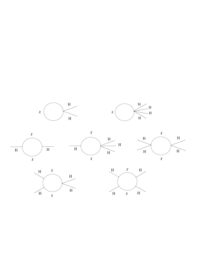
Figure 1: One-loop diagrams. $H=(H^{0},H^{+})$ and $\chi\equiv t,b,T$, with all possible combinations of these particles in the loop diagrams.

By using well known methods it is straightforward to obtain the different contributions after some work. The first one ($k=1$) corresponds to the first two diagrams in Fig. 1 and it is given by:

$$\Delta S^{(1)}[H]=-i\mbox{Tr}(G\hat{I})=-\frac{4}{3}\lambda_{1}\,m_{T}\,f\,s\int d^{4}x\left(\frac{HH^{{\dagger}}}{f^{2}}-\frac{(HH^{{\dagger}})^{2}}{f^{4}}\right)I_{0}(m_{T}^{2})\,,$$ (3.33)

where the divergent integral $I_{0}(m_{T}^{2})$ is:

$$I_{0}(m_{T}^{2})=\int d\tilde{p}\frac{i}{p^{2}-m_{T}^{2}}\,.$$ (3.34)

In order to make sense of this integral we will use an ultraviolet cut-off $\Lambda$, where our effective description of the low energy dynamics breaks down. The result is:

$$I_{0}(m_{T}^{2})=\frac{1}{(4\pi)^{2}}\left[\Lambda^{2}-m_{T}^{2}\log\left(\frac{\Lambda^{2}}{m_{T}^{2}}+1\right)\right]\,.$$ (3.35)

For $k=2$ (see the three generic diagrams on the second line of Fig. 1), one gets:

$$\Delta S^{(2)}[H] = \frac{i}{2}\mbox{Tr}(G\hat{I})^{2}=4\lambda_{1}^{2}\int d^{4}xHH^{{\dagger}}(c^{2}I_{0}(0)+s^{2}I_{0}(m_{T}^{2}))$$ (3.36)

$$+ 2\lambda_{1}^{2}\int d^{4}x\frac{(HH^{{\dagger}})^{2}}{f^{4}}(I_{0}(0)+2m_{T}^{2}s^{2}I_{1}(m_{T}^{2}))$$

$$- \frac{16}{3}\lambda_{1}^{2}\int d^{4}x\frac{(HH^{{\dagger}})^{2}}{f^{4}}(c^{2}I_{0}(0)+s^{2}I_{0}(m_{T}^{2}))\,,$$

where the new divergent integral $I_{1}(m_{T}^{2})$ properly regularized is given by:

$$I_{1}(m_{T}^{2})=\int d\tilde{p}\frac{i}{(p^{2}-m_{T}^{2})^{2}}=-\frac{1}{(4\pi)^{2}}\left[\log\left(\frac{\Lambda^{2}}{m_{T}^{2}}+1\right)-\frac{1}{1+\frac{m_{T}^{2}}{\Lambda^{2}}}\right]\,.$$ (3.37)

The $k=3$ contribution (see the first diagram in the bottom line of Fig. 1) is:

$$\Delta S^{(3)}[H]=-\frac{i}{3}\mbox{Tr}(G\hat{I})^{3}=-8m_{T}\lambda_{1}^{3}s\int d^{4}x\frac{(HH^{{\dagger}})^{2}}{f}(c^{2}I_{2}(m_{T}^{2})+s^{2}I_{1}(m_{T}^{2}))\,,$$ (3.38)

where the divergent integral $I_{2}(m_{T}^{2})$ can be written as:

$$I_{2}(m_{T}^{2})=\int d\tilde{p}\frac{i}{p^{2}(p^{2}-m_{T}^{2})}=-\frac{1}{(4\pi)^{2}}\log\left(\frac{\Lambda^{2}}{m_{T}^{2}}+1\right)\,.$$ (3.39)

Finally, for $k=4$, we get

$$\Delta S^{(4)}[H]=\frac{i}{4}\mbox{Tr}(G\hat{I})^{4}=4\lambda_{1}^{4}\int d^{4}x(HH^{{\dagger}})^{2}(s^{4}I_{1}(m_{T}^{2})+2s^{2}c^{2}I_{2}(m_{T}^{2})+c^{4}I_{2}(0)).$$ (3.40)

Here we need to compute $I_{2}(0).$ This integral is not only ultraviolet-divergent but also infrared-divergent. Thus we need to introduce a new infrared cut-off $m$ (obviously the natural value for this cut-off is of the order of $v,$ i.e. the scale of the electroweak symmetry breaking). Then we find:

$$I_{2}(0)=\int d\tilde{p}\frac{i}{p^{4}}=-\frac{1}{(4\pi)^{2}}\log\left(\frac{\Lambda^{2}}{m^{2}}\right)\,.$$ (3.41)

Therefore, by using the previous results, it is possible to write the Higgs effective potential parameters as :

$$\mu^{2}=N_{c}\frac{m_{T}^{2}\lambda_{t}^{2}}{4\pi^{2}}\log\left(1+\frac{\Lambda^{2}}{m_{T}^{2}}\right),$$ (3.42)

and

$$\lambda = \frac{N_{c}}{(4\pi)^{2}}\left[2(\lambda_{t}^{2}+\lambda_{T}^{2})\frac{\Lambda^{2}}{f^{2}}-\log\left(1+\frac{\Lambda^{2}}{m_{T}^{2}}\right)\left(-\frac{2m_{T}^{2}}{f^{2}}\left(\frac{5}{3}\lambda_{t}^{2}+\lambda_{T}^{2}\right)+4\lambda_{t}^{4}+4(\lambda_{T}^{2}+\lambda_{t}^{2})^{2}\right)\right.$$ (3.43)

$$\left.-4\lambda_{T}^{2}\frac{1}{1+\frac{m_{T}^{2}}{\Lambda^{2}}}\left(\frac{m_{T}^{2}}{f^{2}}-2\lambda_{t}^{2}-\lambda_{T}^{2}\right)-4\lambda_{t}^{4}\log\left(\frac{\Lambda^{2}}{m^{2}}\right)\right],$$

where $N_{c}$ is the number of colors and $\lambda_{t}$ and $\lambda_{T}$ are, respectively, the SM top Yukawa coupling and the heavy top Yukawa coupling, given by :

$$\lambda_{t} = \frac{\lambda_{1}\lambda_{2}}{\sqrt{\lambda_{1}^{2}+\lambda_{2}^{2}}}$$

$$\lambda_{T} = \frac{\lambda_{1}^{2}}{\sqrt{\lambda_{1}^{2}+\lambda_{2}^{2}}}\,.$$ (3.44)

There are several comments about this result which it is worthwhile stressing. First, the effective potential depends on $H$ through the combination $|H|^{2}=HH^{\dagger}$, thus reflecting the fact that the radiative corrections considered preserve the SM $SU(2)_{L}\times U(1)_{Y}$ symmetry. However, $\mu^{2}>0$ and $\lambda>0$, which are the right signs for these corrections to spontaneously break this symmetry down to $U(1)_{\rm{em}}$. Thus the minima of the effective potential occur whenever $|H|^{2}=v^{2}/2\equiv\mu^{2}/(2\lambda)$. By choosing the new vacuum as the state $H=(0,v)/\sqrt{2}$, we recover the above-mentioned SM symmetry breaking. In particular we find that the physical Higgs boson mass is given by $m_{H}^{2}=2\lambda v^{2}$. Notice that for $\lambda<0$ the model would be inconsistent and for $\mu^{2}<0$ there would be no spontaneous symmetry breaking.

In spite of having found apparently the same results as in the SM, there are however a number of nice properties in the LH model. First of all, as we have shown, the Higgs potential parameters can be computed in terms of other more fundamental parameters; therefore do not need to be introduced ad hoc in order to get the appropriate symmetry breaking, as happens in the SM. Moreover, the symmetry breaking appears as a result of the dynamics, through third generation quarks radiative corrections and not as a tree-level consequence of the SM Lagrangian. On the other hand, the Higgs mass can be written as $m_{H}^{2}=2\mu^{2}$ and $\mu^{2}$ is only a logarithmic-divergent quantity. Therefore, the Higgs mass is, not only light as the precision test of the SM seems to suggest, but also free from the undesired quadratic divergences that appear in the original formulation of the SM. Notice also that the quadratic divergences appearing in $\lambda$ do not alter this result.

Once the spontaneous breaking of the SM symmetry is produced, the Yukawa Lagrangian given above gives rise to a new mass matrix for the $t$ and $T$ quarks (the $b$ quark remains massless). This mass matrix can be diagonalized through a rotation of the left chiral states $t_{L}$ and $T_{L}$ given by the angle $\theta_{L}$, which, for $v\ll f,$ can be written as:

$$\sin\theta_{L}\simeq\left(\frac{\lambda_{1}^{2}}{\lambda_{1}^{2}+\lambda_{2}^{2}}\right)\frac{v}{f}$$ (3.45)

and, by other rotation of the right states $t_{R}$ and $T_{R}$, given by the angle $\theta_{R}$

$$\sin\theta_{R}\simeq s\left[1-c^{2}\left(\frac{1}{2}-\left(\frac{\lambda_{1}^{2}}{\lambda_{1}^{2}+\lambda_{2}^{2}}\right)\right)\frac{v^{2}}{f^{2}}\right].$$ (3.46)

After these rotations have been done the new mass eigenvalues become:

$$m_{t}=\lambda_{t}\,v\left[1+\left(-\frac{1}{3}+\frac{1}{2}\frac{\lambda_{1}^{2}}{\lambda_{1}^{2}+\lambda_{2}^{2}}\left(1-\frac{\lambda_{1}^{2}}{\lambda_{1}^{2}+\lambda_{2}^{2}}\right)\right)\frac{v^{2}}{f^{2}}\right]$$ (3.47)

and

$$m_{T}=\frac{\lambda_{t}^{2}+\lambda_{T}^{2}}{\lambda_{T}}f-\frac{1}{2}\frac{\lambda_{1}^{2}}{\sqrt{\lambda_{1}^{2}+\lambda_{2}^{2}}}\left(1-\frac{\lambda_{1}^{2}}{\lambda_{1}^{2}+\lambda_{2}^{2}}\right)\frac{v^{2}}{f}.$$ (3.48)

4 Constraints on the LH parameter space

Whatever model one considers as a candidate for physics beyond the SM, the consistency with present experimental data is a key prediction of that candidate model. It is well known that indirect constraints from precision electroweak measurements on new physics at the TeV scale are severe. There exist several studies of the corrections to electroweak precision observables in the Little Higgs models, exploring whether there are regions of the parameter space in which the model is consistent with data [1, 2, 7, 13, 14, 15, 16].

The effective Higgs potential parameters are related with the vacuum expectation value $v$ through $\mu^{2}=\lambda v^{2}$; with $v\simeq 245$ GeV. By imposing this condition, we could extract crucial information on the allowed region of the parameter space in the LH model. To show this we will consider here the case of the heavy quark contribution to the Higgs potential. In spite of the fact that other contributions coming from gauge bosons, scalars and other higher loops are relevant, the fermionic sector provides a good illustration of the kind of constraints that it will be possible to set on the LH parameter space from the complete effective Higgs potential.

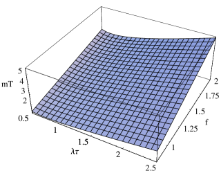
(a)	(b)

Figure 2: (a) $m_{T}$ as a function of $\lambda_{T}$ and $f$, with $0.5<\lambda_{T}<2.5$ and $0.5<f<2$ and (b) $m_{T}$ as a function of $\lambda_{T}$ for $f=1$ TeV.

The contributions from the fermion sector of the model to $\mu^{2}$ and $\lambda$ are summarized in (3.42) and (3.43), respectively; the undetermined parameters of the model are the heavy top mass $m_{T}$, the coupling constant $\lambda_{T}$, the symmetry breaking scale $f$, and the scale $\Lambda$. However, there are several relations between them which are worth remarking on. Firstly, before the electroweak symmetry breaking by radiative corrections, we have:

$$m_{T}=f\,\frac{\lambda_{t}^{2}+\lambda_{T}^{2}}{\lambda_{T}}\,,$$ (4.49)

which could, in principle, be tested by the LHC experiments [2, 8]. This relation is crucial for the cancellation of quadratic divergences contributions to the Higgs boson mass. Besides, considering $m_{T}$ much larger than $2$ TeV would imply a large amount of fine-tuning in the Higgs potential, and thus the heavy top should be below about $2$ TeV ($m_{T}\raisebox{-1.72218pt}{$\stackrel{{\scriptstyle<}}{{\scriptstyle\sim}}$\,}2.5$ TeV) [5, 8]. Note that, since the top-quark mass is already known in the SM, absolute bounds are derived on the couplings, $\lambda_{1},\lambda_{2}\geq m_{t}/v$ or $\lambda_{1}\lambda_{2}\geq 2(m_{t}/v)^{2}$  [7]. As a consequence, we get the bound $\lambda_{T}\raisebox{-1.72218pt}{$\stackrel{{\scriptstyle>}}{{\scriptstyle\sim}}$\,}0.5$, which have been considered in our analysis. For the purpose of illustration, the dependence of $m_{T}$ with $\lambda_{T}$ and $f$ is shown in Fig. 2a for $0.5<\lambda_{T}<2.5$ and $0.8$ TeV $<f<2$ TeV. The corrections decrease with $\lambda_{T}$ having a minimum for a value of the coupling constant closed to $1$, and then they increase. Clearly, $m_{T}$ grows linearly with the parameter $f$, $f\raisebox{-1.72218pt}{$\stackrel{{\scriptstyle<}}{{\scriptstyle\sim}}$\,}1$ TeV being the favored values at this level, because of the condition $m_{T}\raisebox{-1.72218pt}{$\stackrel{{\scriptstyle<}}{{\scriptstyle\sim}}$\,}2$ TeV. For $\lambda_{T}>1.7$ we get values of the heavy top mass above $2$ TeV, when $f=1$ TeV (Fig. 2b). We note that once the spontaneous symmetry breaking of the SM is produced, the heavy top mass is reduced by ${\cal{O}}(v^{2}/f^{2})$ terms (see eq. (3.48)), but the reduction is only of about $0.01$ TeV. Therefore, the previous discussion does not change in a significant way. Secondly, $\Lambda$ is restricted by the suggested condition $\Lambda\sim 4\pi f$ [6] and, as for the scale $\Lambda$, the electroweak precision tests seem to indicate an experimental lower bound $\Lambda\raisebox{-1.72218pt}{$\stackrel{{\scriptstyle>}}{{\scriptstyle\sim}}$\,}10$ TeV [17].

With those possible values of the three parameters $\lambda_{T}$, $f$ and $\Lambda$, we will focus on studying some generic information of the LH model derived from the condition $\mu^{2}=\lambda v^{2}.$ For the numerical analysis, and by taking into account the previous discussion, we varied the above three parameters in the following ranges, $0.5<\lambda_{T}<2$, $10$ TeV $<\Lambda<12$ TeV and, accordingly, $0.8$ TeV $<f<1$ TeV. Let us first describe the behaviour of $\mu^{2}$ with $\lambda_{T}$, $f$ and $\Lambda$. In general, the $\mu^{2}$ corrections increase with $f$ for $0.5<\lambda_{T}<2$, having a minimum for a certain value of $\lambda_{T}$, which corresponds to a minimum for $m_{T}$. These corrections also increase with $\Lambda$, but less dramatically. We find that the lowest value of $\mu$ is $\mu=0.48$ TeV, when $\lambda_{T}=0.72$, $f=0.8$ TeV and $\Lambda=10$ TeV. Notice that, even if $f$ and $\Lambda$ have the expected values for these parameters on the LH models, the minimum possible value for $\mu$ does not correspond to the value of this parameter predicted by the data. We will discuss this point later on.

Once the corrections to the quartic coupling $\lambda$ has also been computed (see (3.43)), the consistency of the LH model is constrained by the non-trivial condition (1.3), as already established. The result for $\lambda$ in (3.43) has not been given so far and, therefore, the relation between $\lambda$ and $\mu$ has not been studied before and one would expect it to put significant constraints on the LH models. In general, the corrections to $\lambda$ grow with the scale $\Lambda$ but, conversely, we find that they decrease with the symmetry breaking scale $f.$ Figure 3 shows the surface of solutions for this non-trivial condition, by considering the above intervals for $\lambda_{T}$, $f$ and $\Lambda$, and by assuming that $0.3$ TeV $<\mu<0.5$ TeV. Clearly, once the condition (1.3) is assumed, the allowed region of the parameter space is considerably reduced. For $\lambda_{T}$, $f$ and $\Lambda$ in the above intervals, there exist just few points of the parameter space that are in agreement with a predictive model. Besides, we stress that the lowest value of $\mu$ that satisfies (1.3) is $\mu=0.52$ TeV, when $f=0.85$ TeV, $\lambda_{T}=0.52$ and $\Lambda=10$ TeV.

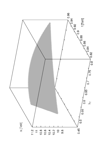
Figure 3: Values of $\Lambda$, $f$ and $\lambda_{T}$, with $0.5<\lambda_{T}<2$, $0.8$ TeV $<f<1$ TeV and $10$ TeV $<\Lambda<12$ TeV, which satisfy the condition $\mu^{2}=v^{2}\lambda$, taking $0.3$ TeV $<\mu<0.5$ TeV.

Finally, it is known that the mass term for the Higgs field is generated at the one-loop level by logarithmically divergent diagrams. The one-loop contribution to the Higgs mass from the top sector is given in eq. (3.42) ($m_{H}^{2}=2\mu^{2}$). The lowest value for $\mu$, which satisfies the condition $\mu^{2}=\lambda v^{2}$, is of the order of $0.5$ TeV. However, it is well known that $\mu$ is forced by data to be at most of order $200$ GeV. Therefore, other contributions must be included in order to obtain the predicted value of $\mu.$ Notice that the Higgs mass parameter in the LH model also receives contributions (not included here) from the vector bosons sector (1-loop correction) and from the scalar sector (2-loop correction), which are opposite in sign to the top-fermion contribution. We discuss in the following how the vector boson contributions could reduce the value of $\mu$ to its allowed value.

Concerning the gauge bosons interactions, we consider the two different models that have been described in Section 2: the original LH with two $U(1)$ groups (model I) and the other one with just one $U(1)$ group (model II). Once the quantum corrections involving gauge interactions are included, the logarithmically enhanced contributions of the vector bosons to the mass term of the Higgs field in each model are given, respectively, and at one-loop level, by

$$\mu^{2\,\,\,{\it{I}}}_{{\mbox{g}}}=-\frac{3}{64\pi^{2}}\left(3g^{2}M_{W^{\prime}}^{2}\log\left(\frac{\Lambda^{2}}{M_{W^{\prime}}^{2}}+1\right)+g^{\prime 2}M_{B^{\prime}}^{2}\log\left(\frac{\Lambda^{2}}{M_{B^{\prime 2}}}+1\right)\right)\,,$$ (4.50)

$$\mu^{2\,\,\,{\it{II}}}_{{\mbox{g}}}=-\frac{3}{64\pi}\left(3g^{2}M_{W^{\prime}}^{2}\log\left(\frac{\Lambda^{2}}{M_{W^{\prime}}^{2}}+1\right)+g^{\prime 2}\Lambda^{2}\right)\,,$$ (4.51)

where $M_{W^{\prime}}$ and $M_{B^{\prime}}$ are the heavy gauge boson masses,

$$M_{W^{\prime}}=\frac{fg}{2\cos\psi\sin\psi}\hskip 14.45377pt\mbox{and}\hskip 14.45377ptM_{B^{\prime}}=\frac{fg^{\prime}}{\sqrt{20}\cos\psi^{\prime}\sin\psi^{\prime}}\,;$$ (4.52)

with $\psi$ and $\psi^{\prime}$ being the mixing angles for the $W^{\prime}$ and $B^{\prime}$ states. Note that the different results for these two models comes from the fact that there is no $B^{\prime}$ in model II.

Let us now estimate the cancellations that could occur between the fermion sector and the vector boson sector by keeping $\mu^{2}$ of order 200 GeV and, therefore, $m_{H}$ light. For the numerical analysis, we varied the $\lambda_{T}$, $f$ and $\Lambda$ parameters in the intervals given before.

For model I, in order to avoid the gauge masses being too small or too big, we impose that $0.1<\cos\psi<0.9$ and $0.1<\cos\psi^{\prime}<0.4$. Once cancellations occurs, we find that the lowest value for $\mu$ is $0.338$ TeV for $\lambda_{T}\simeq 0.7$, $f\simeq 0.8$ TeV, $\Lambda\simeq 10$ TeV, $\cos\psi\simeq 0.1$, and $\cos\psi^{\prime}\simeq 0.1$. On the other hand, in the case of model II, by considering the same numerical values as above, we obtain better results. The lowest value for $\mu$ is now of order of $0.2$ TeV, with $\lambda_{T}\simeq 0.65$, $f\simeq 0.8$ TeV, $\Lambda\simeq 11.9$ TeV, and $\cos\psi\simeq 0.1.$ Therefore, we find that the so-called model II is more effective than model I from the point of view of cancellations between different sectors of the LH model.

From the above results, we could conclude that the condition $\mu^{2}=\lambda v^{2}$ is very important in the analysis of predictions from the LH model, and that the inclusion of the contributions from the vector bosons on both $\mu$ and $\lambda$ will be crucial to increase the allowed region of the parameter space. To explore the complete region of the parameter space in which the LH model is consistent with the data, we plan to make the full analysis with the inclusion of contributions from all the sectors of the model [18].

5 Conclusions

In the SM the Higgs mass $m_{H}$ receives quadratic radiative corrections coming from the gauge bosons, the Higgs self-coupling $\lambda$ and from the top quark (the latter being negative). The requirement of not having one-loop contributions to the squared Higgs mass larger than $10\%$ of the tree-level value, and the experimental constraint $115$ GeV $<m_{H}<200$ GeV, sets the SM ultraviolet cut-off $\Lambda_{\rm{SM}}$ to be lesser than $2$ or $3$ TeV. However, to avoid conflict with electroweak precision observables, a scale of the order of $10$ TeV seems to be needed. This is the so called little hierarchy problem which the LH model pretends to solve.

In this work we have computed and analyzed the fermion contributions to the low energy Higgs effective potential and we have illustrated the kind of constraints on the possible values of the LH parameters that can be set by requiring the complete LH Higgs effective potential to reproduce exactly the SM potential. The analysis we have done is relevant whenever one assumes that the new physics decouples from the low energy physics. Our results are compatible with the LH model solving the little hierarchy problem, but the region of LH model parameter space compatible with this possibility probably is not very large.

We have explored the region of the $\lambda_{T}$, $f$ and $\Lambda$ parameter space compatible with the condition $\mu^{2}=\lambda v^{2}$, taking $m_{T}\leq 2$ TeV, $\Lambda\thicksim 4\pi f$, and also imposing the requirement of having $\mu$ smaller than $0.5$ TeV. The scales $f$ and $\Lambda$ run around the typical scales predicted by the LH models. For this purpose we have computed the fermion contributions to the quartic coupling $\lambda$ at the one-loop level. Since the values obtained for $\mu$ are relatively high, the inclusion of the gauge and the scalar sector of the model is needed to reduce $\mu$ to its expected value. Therefore, more detailed computations, including the full one-loop gauge boson and the relevant two-loop Goldstone boson contribution, are needed in order to establish definitely the validity of the LH model and its compatibility with the present phenomenological constraint including the precise form of the Higgs potential. Work is in progress in this direction [18].

References

- [1] M. Schmaltz, D. Tucker-Smith, Ann. Rev. Nucl. Part. Sci. 55, 229 (2005), hep-ph/0502182.
- [2] M. Perelstein, hep-ph/0512128 (submitted to Prog.Part.Nucl.Phys.).
- [3] H. Georgi, A. Pais, Phys. Rev. D10, 539 (1974) and D12, 508 (1975).
- [4] M. J. Dugan, H. Georgi, D. B. Kaplan, Nucl. Phys. B 254, 299 (1985); H. Georgi, D. B. Kaplan, Phys. Lett. B 145, 216 (1984) and 136, 183 (1984); H. Georgi, D. B. Kaplan, P. Galison, Phys. Lett. B 143, 152 (1984); D. B. Kaplan, H. Georgi, S. Dimopoulos, Phys. Lett. B 136, 187 (1984); S. Dimopoulos, J. Preskill, Nucl. Phys. B 199, 206 (1982).
- [5] N. Arkani-Hamed, A.G. Cohen, E. Katz, A.E. Nelson, JHEP 0207, 034 (2002), hep-ph/0206021.
- [6] A. Manohar, H. Georgi, Nucl. Phys. B234, 189 (1984); M. A. Luty, Phys. Rev. D57, 1531 (1998), hep-ph/9706235; A. G. Cohen, D. B. Kaplan, A. E. Nelson, Phys. Lett. B412, 301 (1997), hep-ph/9706275.
- [7] T. Han, H. E. Logan, B. McElrath, L. T. Wang, Phys. Rev. D67, 095004 (2003), hep-ph/0301040.
- [8] M. Perelstein, M. Peskin, A. Pierce, Phys. Rev. D69, 075002 (2004), hep-ph/0310039.
- [9] I. Low, W. Skiba, D. Smith, Phys. Rev. D66, 072001 (2002), hep-ph/0207243; D. E. Kaplan, M. Schmaltz, JHEP 0310, 039 (2003), hep-ph/0302049; S. Chang, J. G. Wacker, Phys. Rev. D69, 035002 (2004), hep-ph/0303001; W. Skiba, J. Terning, Phys. Rev. D68, 075001 (2003), hep-ph/0305302; S. Chang, JHEP 0312, 057 (2003), hep-ph/0306034.
- [10] J.A. Casas, J.R. Espinosa, I. Hidalgo, JHEP 0503, 038 (2005), hep-ph/0502066.
- [11] F. Bazzocchi, M. Fabbrichesi, M. Piai, Phys. Rev. D72 (2005) 095019, hep-ph/0506175.
- [12] A. Dobado, A. Gómez-Nicola, A.L. Maroto, J.R. Peláez, Effective Lagrangians for the Standard Model (Springer-Verlag, Heidelberg, 1997).
- [13] Z. Han, W. Skiba, Phys. Rev. D72, 035005 (2005), hep-ph/0506206; H.E. Logan, Phys. Rev. D70, 115003 (2004), hep-ph/0405072; T. Han, H. E. Logan, B. McElrath, L. T. Wang, Phys. Lett. B563, 191 (2003) [Erratum-ibid. B603, 257 (2004)], hep-ph/0302188.
- [14] C. Csaki, J. Hubisz, G. D. Kribs, P. Meade, J. Terning, Phys. Rev. D67 115002 (2003), hep-ph/0211124, and D68, 035009 (2003), hep-ph/0303236; J. L. Hewett, F. J. Petriello, T. G. Rizzo, JHEP 0310, 062 (2003), hep-ph/0211218.
- [15] T. Gregoire, D. R. Smith, J. G. Wacker, Phys. Rev. D69, 115008 (2004), hep-ph/0305275; M. C. Chen and S. Dawson, Phys. Rev. D70, 015003 (2004), hep-ph/0311032; W. Kilian, J. Reuter, Phys. Rev. D70, 015004 (2004), hep-ph/0311095; G. Marandella, C. Schappacher, A. Strumia, Phys. Rev. D72, 035014 (2005), hep-ph/0502096.
- [16] M.C. Chen, Mod. Phys. Lett. A21, 621 (2006), hep-ph/0601126; S.R. Choudhury, A.S. Cornell, N. Gaur, A. Goyal, hep-ph/0604162; J.A. Conley, J. Hewett, M. P. Le, Phys. Rev. D72, 115014 (2005), hep-ph/0507198; C.O. Dib, R. Rosenfeld, A. Zerwekh, AIP Conf. Proc. 815, 296 (2006), hep-ph/0509013; Z. Berezhiani, P.H. Chankowski, A. Falkowski, S. Pokorski, Phys. Rev. Lett. 96, 031801 (2006), hep-ph/0509311.
- [17] R. Barbieri, A. Strumia, hep-ph/0007265; R. Barbieri, A. Pomarol, R. Rattazzi, A. Strumia, Nucl. Phys. B703, 127 (2004), hep-ph/0405040.
- [18] A. Dobado, L. Tabares, S. Peñaranda, Phys. Rev. D75 (2007) 083527, hep-ph/0612131.