The Modern Description of Semileptonic Meson Form Factors

Abstract

I describe recent advances in our understanding of the hadronic form factors governing semileptonic meson transitions. The resulting framework provides a systematic approach to the experimental data, as a means of extracting precision observables, testing nonperturbative field theory methods, and probing a poorly understood limit of QCD.

I Introduction: into the meson

Semileptonic transitions of one meson into another yield important measurements of both weak and strong dynamics. By comparing the experimentally determined decay rate to a theoretical normalization of the relevant hadron transition amplitude at one or more kinematic points, elements of the Cabibbo-Kobayashi-Maskawa (CKM) matrix are determined. Independent of the overall normalization, the shape of the semileptonic spectrum provides a quantitative probe of underlying hadron dynamics.

Of the six CKM elements that can be probed directly using stable hadrons, determinations from exclusive semileptonic transitions are the most precise ($|V_{us}|$); competitive with other determinations ($|V_{ub}|$, $|V_{cb}|$ from inclusive semileptonic $B$ decays; $|V_{cd}|$ from deep-inelastic neutrino scattering; $|V_{cs}|$ from charm-tagged $W$ decays); or complementary to existing determinations ($|V_{ud}|$, from nuclear beta decay) Eidelman:2004wy . In all cases, the theoretical normalization gives a dominant error. The experimentally determined spectrum can be used both to test the nonperturbative methods used in determining this normalization, and to optimize the merger of theory with experiment.

For the study of hadron dynamics, the use of a virtual $W$ boson probe in semileptonic transitions can be viewed in analogy with the use of a virtual photon in deep-inelastic scattering. The “known” and theoretically “clean” weak (electromagnetic) physics is used to probe the “unknown” and theoretically “messy” strong physics of the meson (proton). For the case of semileptonic transitions, in addition to the virtuality of the exchanged boson, we can envision “dialing the knobs” of the initial- and final-state meson masses. To be precise, consider the situation pictured in Fig. 1. A $Q\bar{q}$ pair with quantum numbers of the “heavy” meson $H$ is created at spacetime point $x$, interacts with a flavor-changing current at $y$, and the $q^{\prime}\bar{q}$ pair with quantum numbers of the “light” meson $L$ is annihilated at $z$. By suitable manipulations , we can extract hadronic transition amplitudes (form factors) from this correlation function. The entire process takes place in the complicated QCD background with soft and hard gluons interacting with everything, $q\bar{q}$ pairs popping out of the vacuum, etc. On this fixed background, we can compute a correlation function with any quark masses we desire; in fact Nature has chosen a few fixed values (and presumably obtained the correct answer), and we shall be content with these. 

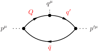
Figure 1: Correlation function from which the semileptonic form factors are extracted. $Q$, $q^{\prime}$ and $q$ are quark labels. $p^{\mu}$, $p^{\prime\mu}$ and $q^{\mu}$ are momenta.

In this way, a rather complete exploration of the “1-body” semileptonic topology, summarized by invariant form factors $F(m_{H},m_{L},q^{2})$, is possible. A similar analysis can be applied to “0-body” leptonic decays, and to “2-body” hadronic decays. The former case is rather simple: by kinematics there is only the single “knob” of the meson mass, and the result is summarized by a single number, the decay constant $f(m_{H})$. The latter case is rather complicated, with many different topologies contributing to a typical physical process Buras:1998ra .

The remainder of the talk is organized as follows. Section II reviews the first-principles knowledge we have about the form factors, following just from kinematics without dynamics. Pseudoscalar-pseudoscalar transitions between “heavy-light”, nonsinglet mesons are particularly simple and are the main focus.  Rigorous power-counting arguments provide the basis for a powerful expansion based on analyticity. Section III illustrates how the experimental data is simplified by making use of this expansion. In particular, we find the remarkable conclusion that in terms of standard variables, no semileptonic meson form factor has ever been observed to deviate from a straight line. Given that the form factors are indistinguishable from straight lines, if the shape of the semileptonic spectrum is to provide insight on QCD, it must be through the slope of the form factor; in fact, a clear but unsolved question in QCD translates directly into the numerical value of this slope in an appropriate limit, as described in Section IV. Phenomenological implications in the $B\to\pi$ system are considered in Section V. The methodology described here provides a convenient framework in which to understand precisely what measurements in the charm system can, and cannot, say that is relevant to the bottom system, as discussed in Section VI. Section VII outlines the extension to pseudoscalar-vector transitions.

II Analyticity and crossing symmetry

An oft-cited downside of old and well-known dispersion-relation arguments is that the results are too general, and do not make specific predictions for detailed dynamics. In fact, precisely these properties make them useful to the problem at hand—it is essential to make some statement on the possible functional form of the form factors, yet we do not want to make assumptions, explicit or implicit, on the dynamics.

Table 1: Maximum $|z(t,t_{0})|$ throughout semileptonic range with symmetrizing choice $t_{0}=t_{+}(1-\sqrt{1-t_{-}/t_{+}})$.

Process	CKM element	$|z|_{\rm max}$
$\pi^{+}\to\pi^{0}$	$V_{ud}$	$3.5\times 10^{-5}$
$B\to D$	$V_{cb}$	0.032
$K\to\pi$	$V_{us}$	0.047
$D\to K$	$V_{cs}$	0.051
$D\to\pi$	$V_{cd}$	0.17
$B\to\pi$	$V_{ub}$	0.28

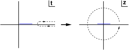
Figure 2: Mapping (3) of the cut $t$ plane onto the unit circle. The semileptonic region is represented by the blue line.

The analytic structure of the form factors can be investigated by standard means.  Let us focus on the form factors for pseudoscalar-pseudoscalar transitions, defined by the matrix element of the relevant weak vector current, ($q\equiv p-p^{\prime}$)

$$\langle L(p^{\prime})|V^{\mu}|H(p)\rangle$$

$$\quad=F_{+}(q^{2})\left(p^{\mu}+p^{\prime\mu}\right)+F_{-}(q^{2})q^{\mu}$$

$$\quad=F_{+}(q^{2})\left(p^{\mu}+p^{\prime\mu}-{m_{H}^{2}-m_{L}^{2}\over q^{2}}q^{\mu}\right)$$

$$\qquad\qquad+F_{0}(q^{2}){m_{H}^{2}-m_{L}^{2}\over q^{2}}q^{\mu}\,.$$ (1)

To ensure that there is no singularity at $q^{2}=0$, the form factors obey the constraint

$$F_{+}(0)=F_{0}(0)\,.$$ (2)

Ignoring possible complications from anomalous thresholds or subthreshold resonances, to be discussed below, the form factors $F(t=q^{2})$ can be extended to analytic functions throughout the complex $t$ plane, except for a branch cut along the positive real axis, starting at the point $t=t_{+}$ [$t_{\pm}\equiv(m_{H}\pm m_{L})^{2}$] corresponding to the threshold for production of real $\bar{H}L$ pairs in the crossed channel. By a standard transformation, as illustrated in Figure 2, the cut $t$ plane is mapped onto the unit circle $|z|\leq 1$,

$$z(t,t_{0})\equiv{\sqrt{t_{+}-t}-\sqrt{t_{+}-t_{0}}\over\sqrt{t_{+}-t}+\sqrt{t_{+}-t_{0}}}\,,$$ (3)

where $t_{0}$ is the point mapping onto $z=0$. The isolation of the semileptonic region from singularities in the $t$ plane implies that $|z|<1$ throughout this region. Choosing $t_{0}=t_{+}(1-\sqrt{1-t_{-}/t_{+}})$ minimizes the maximum value of $|z|$; for typical decays these maximum values are given in Table 1.

Since the form factor is analytic, it may be expanded,

$$F(t)={1\over P(t)\phi(t,t_{0})}\sum_{k=0}^{\infty}a_{k}(t_{0})z(t,t_{0})^{k}\,,$$ (4)

where $P$ and $\phi$ will be explained shortly. From Table 1, it is apparent that if some control over the coefficients $a_{k}$ can be established, the expansion is rapidly convergent.

To bound the coefficients appearing in (4), we consider the norm,

$$||F||^{2} \equiv \sum_{k=0}^{\infty}a_{k}^{2}={1\over 2\pi i}\oint{dz\over z}|P\phi F|^{2}$$ (5)

$$= {1\over\pi}\int_{t_{+}}^{\infty}{dt\over t-t_{0}}\sqrt{t_{+}-t_{0}\over t-t_{+}}|P\phi F|^{2}\,.$$

By crossing symmetry, the norm can be evaluated using the form factors for the related process of $\bar{H}L$ production.

II.1 Subthreshold poles, (absence of) anomalous thresholds, and a choice of $P$

For some hadronic processes, it may happen that subthreshold resonances occur in the production amplitude, which must be properly taken into account. Particles lying below threshold are hadronically stable, so that ignoring higher-order weak and electromagnetic corrections, they are described by simple poles. The canonical example is the $B^{*}$ pole appearing in the vector channel for $B\to\pi$. Such poles could in principle be simply subtracted, but doing so requires knowledge of the relevant coupling appearing as the coefficient of $1/(m_{B^{*}}^{2}-t)$ in the dispersive representation of the form factor. Armed with only the knowledge of the pole position, this pole can instead be removed by multiplying with a function $P(t)$ with a simple zero at $m_{B^{*}}^{2}$. Requiring also that the function satisfy $|P|=1$ along the cut, up to an arbitrary phase,

$$P_{F_{+}}^{B\to\pi}(t)=z(t,m_{B^{*}}^{2})\,,$$ (6)

with $z$ as in (3).

It may happen in some processes that “anomalous thresholds” appear. The relevant aspects of this technical subject can be summarized as follows: an anomalous threshold can occur in the spacelike region, $t<0$, only if $H$ and $L$ are unstable, i.e., $m_{H\,{\rm or}\,L}>m_{X}+m_{Y}$ for some hadrons $X$ and $Y$ coupling to $H$ or $L$. Similarly, an anomalous threshold can occur in the timelike region, $t_{-}<t<t_{+}$, only if $m_{H\,{\rm or}\,L}^{2}>m_{X}^{2}+m_{Y}^{2}$.  This explains the priveleged position of ground-state heavy-light pseudoscalar mesons. The ground state meson with given flavor quantum numbers is necessarily pseudoscalar Weingarten:1983uj . The mesons $H$ and $L$ are therefore the lightest hadrons containing their respective “heavy” quarks, so that in particular $m_{H\,{\rm or}\,L}<m_{X}+m_{Y}$ and $m_{H\,{\rm or}\,L}^{2}<m_{X}^{2}+m_{Y}^{2}$ for any hadrons $X$ and $Y$ containing the same heavy quark.  (For the present purposes, this can be taken as the definition of a “heavy-light” meson.) Fortunately, and for related reasons, these mesons are easily produced and studied experimentally, and in lattice simulations.

II.2 Unitarity and a choice of $\phi$

Nothing in (4) or (5) yet singles out a choice of $\phi$; indeed any analytic function will work, (of which there are many!). A default choice is determined from arguments based on unitarity: by an appropriate choice of $\phi$, the norm can be identified as a partial rate for some inclusive process that is perturbatively calculable. In particular, from

$$\!\!\Pi^{\mu\nu}(q) \equiv i\int d^{4}x\,e^{iq\cdot x}\langle 0|T\left\{V^{\mu}(x)V^{\nu\dagger}(0)\right\}|0\rangle$$ (7)

$$= (q^{\mu}q^{\nu}-g^{\mu\nu}q^{2})\Pi_{1}(q^{2})+q^{\mu}q^{\nu}\Pi_{0}(q^{2})\,,$$

unsubtracted dispersion relations can be written for the quantities ($Q^{2}=-q^{2}$)

$$\chi_{F_{+}}(Q^{2}) = {1\over 2}{\partial^{2}\over\partial(q^{2})^{2}}\left[q^{2}\Pi_{1}\right]={1\over\pi}\int_{0}^{\infty}\!dt\,{t{\rm Im}\Pi_{1}(t)\over(t+Q^{2})^{3}}\,,$$

$$\chi_{F_{0}}(Q^{2}) = {\partial\over\partial q^{2}}\left[q^{2}\Pi_{0}\right]={1\over\pi}\int_{0}^{\infty}\!dt\,{t{\rm Im}\Pi_{0}(t)\over(t+Q^{2})^{2}}\,.$$

Noticing that for $t>t_{+}$, ($\eta$ an isospin factor)

$${\eta\over 48\pi}{[(t-t_{+})(t-t_{-})]^{3/2}\over t^{3}}|F_{+}(t)|^{2} \leq {\rm Im}\Pi_{1}(t)\,,$$

$${\eta t_{+}t_{-}\over 16\pi}{[(t-t_{+})(t-t_{-})]^{1/2}\over t^{3}}|F_{0}(t)|^{2} \leq {\rm Im}\Pi_{0}(t)\,,$$ (9)

shows that an upper bound on the norm can be established by choosing [recall that $|z|=1$ along the integration contour in (II.2)]

$$\phi_{F_{+}}(t,t_{0}) = \sqrt{\eta\over 48\pi}{t_{+}-t\over(t_{+}-t_{0})^{1/4}}\left(z(t,0)\over-t\right)$$

$$\times\left(z(t,-Q^{2})\over-Q^{2}-t\right)^{3/2}\left(z(t,t_{0})\over t_{0}-t\right)^{-1/2}$$

$$\times\left(z(t,t_{-})\over t_{-}-t\right)^{-3/4}\,,$$

$$\phi_{F_{0}}(t,t_{0}) = \sqrt{\eta t_{+}t_{-}\over 16\pi}{\sqrt{t_{+}-t}\over(t_{+}-t_{0})^{1/4}}\left(z(t,0)\over-t\right)$$ (10)

$$\times\left(z(t,-Q^{2})\over-Q^{2}-t\right)\left(z(t,t_{0})\over t_{0}-t\right)^{-1/2}$$

$$\times\left(z(t,t_{-})\over t_{-}-t\right)^{-1/4}\,.$$

The choice of subtracted dispersion relation in (II.2) leads to a “default” choice for $\phi$ in (II.2). With this choice, power counting shows that $a_{k}/a_{0}$ and $\sum_{k}(a_{k}^{2}/a_{0}^{2})$ do not scale as powers of large ratios such as $Q/\Lambda_{\rm QCD}$, or $m_{Q}/\Lambda_{\rm QCD}$ when a heavy-quark mass is present Becher:2005bg . This ensures that there is no parametric enhancement of the coefficients $a_{k}$ that could offset the smallness of $z^{k}$ in the series (4). In fact, at sufficiently large $k$ the coefficients must decrease in order that the sum of squares converge. These properties [analyticity, and $a_{k}/a_{0}\sim\sum_{k}a_{k}^{2}/a_{0}^{2}\sim{\cal O}(1)$ ] are all that is required from the choice of $\phi$. The “physical” prescription following from (II.2), (II.2) and (II.2) automatically ensures that this is the case.

The original motivation for considering the operator product expansion (OPE) in (7) is to place a restriction on the coefficients in (5) according to ($\chi=\chi_{F_{+,0}}$ as appropriate)

$$\sum_{k=0}^{\infty}a_{k}^{2}\leq\chi(Q^{2})\,.$$ (11)

However, in order that an OPE expansion for $\chi(Q^{2})$ converge, $Q^{2}$ (or $m_{Q}^{2}+Q^{2}$ when a heavy-quark is present) must necessarily be large compared to $\Lambda_{\rm QCD}$. This results in a bound that is typically overestimated by some power of the large ratio of perturbative to hadronic scales. In practice, the numerical value for the bound (11) itself is largely irrelevant. What is important is that the choice of $\phi$ which it motivates has the desired properties.

Having chosen a “default” $\phi$, for definiteness, we will also take $Q=0$ in (II.2) as the “default” choice, and where a particular choice is necessary, $t_{0}=t_{+}(1-\sqrt{1-t_{-}/t_{+}})$.

III What the data say

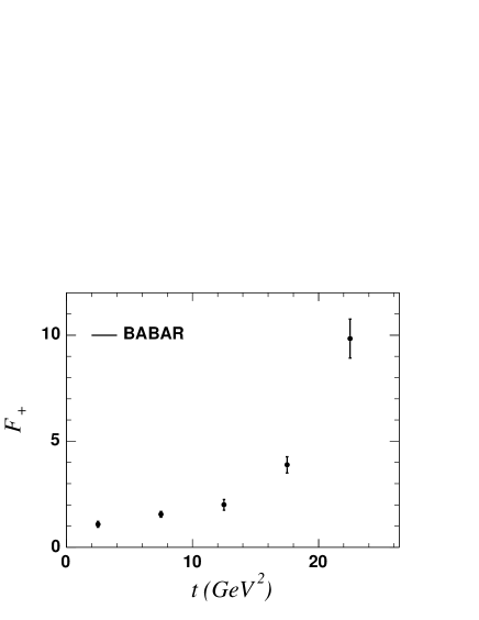
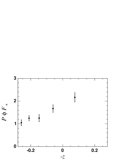
Figure 3: Experimental data for $F_{+}$ in $B\to\pi\ell\nu$, as a function of $t$, and for the function $P\phi F_{+}$ as a function of $z$. Partial branching fractions have been converted to values of the form factor at the midpoint of each bin in $t$ from Aubert:2005cd . Units on the vertical axis are arbitrary (approximately normalized to unity at $t=0$).

Table 2: Linear expansion coefficient $a_{1}/a_{0}$ from (4) at $t_{0}=t_{+}(1-\sqrt{1-t_{-}/t_{+}})$ and $Q=0$.

Process	$a_{1}/a_{0}$	Reference
$B\to D$	$-2.6\pm 2.3$	Abe:2001yf
$K^{+}\to\pi^{0}$	$-0.2\pm 0.2$	Yushchenko:2004zs
$K_{L}\to\pi^{\pm}$	$-0.5\pm 0.2$	Alexopoulos:2004sy
	$\phantom{-}0.0\pm 0.3$	Lai:2004kb
	$-0.2\pm 0.2$	Ambrosino:2006gn
$D\to K$	$-2.7\pm 0.5\pm 0.4$	Huang:2004fr
	$-2.2\pm 0.4\pm 0.4$	Link:2004dh
	$-3.2\pm 0.5\pm 0.2$	Abe:2005sh
$D\to\pi$	$-2.3\pm 0.7\pm 1.3$	Huang:2004fr
	$-1.6\pm 0.5\pm 1.0$	Abe:2005sh
$B\to\pi$	$-1.3\pm 0.6\pm 2.3$	Athar:2003yg
	$-1.9\pm 0.3\pm 1.1$	Aubert:2005cd
	$-1.3\pm 0.8\pm 2.2$	Abe:2004zm

Table 1 can be used to predict the level of precision at which slope, curvature, and higher-order corrections can be resolved by the data. With the “default” values of $Q$ and $t_{0}$, Table 2 shows the results for $a_{1}/a_{0}$ obtained from data. Except where indicated, modes related by isospin are combined. For the $K\to\pi$ case, the results of Yushchenko:2004zs ; Alexopoulos:2004sy ; Lai:2004kb ; Ambrosino:2006gn were presented as a simple quadratic Taylor expansion of the form factor about $t=0$.  These results have been converted to the quadratic $z$ parameterization in (4), by identifying the Taylor series at $t=0$, and propagating errors linearly. For $B\to D$, the results of Abe:2001yf were presented in terms of a parameterization obtained by expanding $\phi$ and $P$ as a Taylor series in $z$ Caprini:1997mu . The result in Table 2 is obtained by converting to the linear $z$ parameterization in (4), with three subthreshold “$B_{c}^{*}$” poles located at $m=6.337,6.899,7.012\,{\rm GeV}$ Caprini:1997mu ; Eichten:1994gt , and then identifying the coefficients in a Taylor series at $t=t_{+}(1-\sqrt{1-t_{-}/t_{+}})$. The results for $D\to K$, $D\to\pi$ and $B\to\pi$ were obtained by fitting the linear $z$ parameterization in (4) to the data. A second error is included by redoing the fits with the quadratic $z$ parameterization, subject to the conservative bound $|a_{k}/a_{0}|<10$. Due to the smallness of $z$ for pion beta decay, $\pi^{+}\to\pi^{0}$ (cf. Table 1), the slope in this case is orders of magnitude from being measured experimentally Cirigliano:2002ng .

At least through linear order, there is no evidence of anomalously large coefficients that could upset the power counting. While it would be desirable to push to the next order and examine the size of $a_{2}/a_{0}$, comparison to data establishes the remarkable conclusion that form-factor curvature has not yet been seen in any semileptonic transition. In fact, for many cases, a form factor slope has yet to be measured. An example of the transformed form factor is illustrated for $B\to\pi$ in Fig. 3.

From the amusing coincidence that $z^{DK}/z^{D\pi}\sim|V_{cd}|/|V_{cs}|$, and $z^{BD}/z^{B\pi}\sim|V_{ub}|/|V_{cb}|$, it turns out that the higher statistics of the Cabibbo-allowed modes ($B\to D$, $D\to K$) are offset at linear order by the smallness of $z$. It is thus likely that curvature will eventually be measured first in the Cabibbo-suppressed modes ($B\to\pi$, $D\to\pi$).

The results in Table 2 are by no means the final word on these quantities, but illustrate the main point, that there is no sign that the $z$ expansion is breaking down. It is also easy to see that unitarity has very little impact. For example, for $B\to\pi$, the bound on $F_{+}$ taken from the OPE at $Q=0$ is overestimated by a factor $\sim(m_{b}/\Lambda_{\rm QCD})^{3}$ Becher:2005bg . Taking for definiteness, $F_{+}(t_{0}=16\,{\rm GeV})\approx 0.8$, the unitarity bound tells us only that $\sum_{k}a_{k}^{2}/a_{0}^{2}\lesssim 2500$ Lellouch:1995yv ; Fukunaga:2004zz ; Arnesen:2005ez . For $B\to D$, at $Q=0$ with the approximate symmetry relation $F_{+}(t_{-})\approx(m_{B}+m_{D})/2\sqrt{m_{B}m_{D}}$, and including three subthreshold poles as in (6), the unitarity bound is overestimated by a factor $\sim(m_{b}/m_{c})^{3}$ and yields $\sum_{k}a_{k}^{2}/a_{0}^{2}\lesssim 9000$ Lellouch:1995yv ; Caprini:1997mu . While these bounds can be improved somewhat by subtracting off subthreshold poles, extending isospin $SU(2)$ to $SU(3)$ flavor symmetry, or by lowering $Q^{2}$, all of these modifications introduce their own uncertainties. 

IV A fundamental question

Given that the form factors (after extracting standard kinematic factors, and expressing them in terms of the appropriate standard variable) are so far indistinguishable from a straight line, it is apparent that any insight to be gained from the shape of the form factors, whether it be tests of nonperturbative methods, inputs to other processes, or more fundamental questions about QCD, must be based in first approximation on the slope of the form factor. In fact, this quantity does provide a clear test of lattice QCD, is an important input to hadronic $B$ decays, and in an appropriate limit can provide the answer to a longstanding open question about the QCD dynamics governing form factors.

It is convenient to define the physical shape observables in terms of the form factor slopes at $t=0$ Hill:2005ju ,

$${1\over\beta} \equiv {m_{H}^{2}-m_{L}^{2}\over F_{+}(0)}\left.dF_{0}\over dt\right|_{t=0}\,,$$

$$\delta \equiv 1-{m_{H}^{2}-m_{L}^{2}\over F_{+}(0)}\left(\left.dF_{+}\over dt\right|_{t=0}-\left.dF_{0}\over dt\right|_{t=0}\right)$$ (12)

$$\equiv {F_{+}(0)+F_{-}(0)\over F_{+}(0)}\,.$$

The quantities $\beta$ and $\delta$ depend only on the masses of the mesons involved.  Being physical quantities, they are independent of any renormalization scale or scheme. As discussed in the introduction, these quantities take definite values for all $m_{H}$ and $m_{L}$, values that are accessible experimentally at the fixed masses $m_{\pi}$, $m_{K}$, $m_{D}$ and $m_{B}$. 

Due to the kinematic constraint (2), the difference of form factor slopes is particularly simple. Firstly, for $m_{H}=m_{L}$,

$$\delta(m_{L},m_{H})=1\,,\quad[m_{H}=m_{L}]\,.$$ (13)

This is the statement of current conservation ($F_{-}=0$) in (II). There are three further distinct limits that we can consider: $m_{H},m_{L}\gg\Lambda_{\rm QCD}$, $m_{H},m_{L}\ll\Lambda_{\rm QCD}$, and $m_{H}\gg\Lambda_{\rm QCD}\gg m_{L}$. Each limit provides valuable insight, and we consider each in turn.

IV.1 $m_{H},m_{L}\gg\Lambda_{\rm QCD}$: HQET

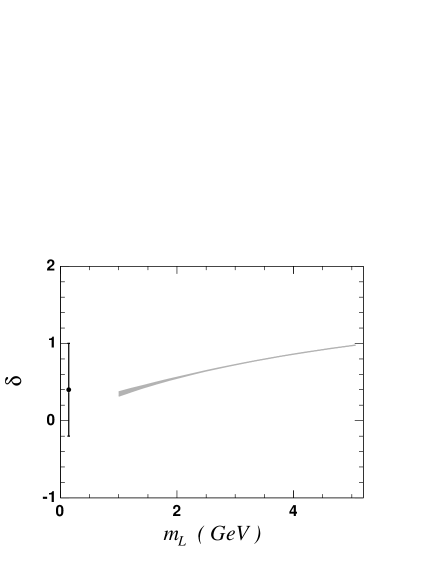
Figure 4: $\delta$ as a function of light-meson mass for fixed heavy-meson mass $m_{H}=m_{B}$. The shaded band gives the prediction from HQET valid for $m_{H}\gtrsim 1\,{\rm GeV}$. The dot with error bars is from experimental data as discussed in the text.

For $m_{H},m_{L}\gg\Lambda_{\rm QCD}$, it is convenient to express the form factors $F_{\pm}$ in terms of reduced amplitudes, $h_{\pm}$ where the dominant heavy-quark mass dependence is extracted: [cf. (II)]

$$F_{+}(p+p^{\prime})+F_{-}(p-p^{\prime})$$

$$\quad\equiv\sqrt{m_{H}m_{L}}\left[h_{+}(v+v^{\prime})+h_{-}(v-v^{\prime})\right]\,,$$ (14)

where the meson velocities are $m_{H}v\equiv p$, $m_{L}v^{\prime}\equiv p^{\prime}$. With these definitions, before any approximation,

$$\delta(m_{L},m_{H})\equiv{2m_{L}\over m_{H}+m_{L}}{1+{h_{-}\over h_{+}}\over 1-{m_{H}-m_{L}\over m_{H}+m_{L}}{h_{-}\over h_{+}}}\,.$$ (15)

At leading power, $h_{+}\approx\xi$, the universal Isgur-Wise function Isgur:1989ed , and $h_{-}\approx 0$, so that

$$\delta(m_{L},m_{H}) = {2m_{L}\over m_{H}+m_{L}}\big{[}1+{\cal O}(\alpha_{s},\Lambda/m_{L},\Lambda/m_{H})\big{]}\,,$$ (16)

$$\quad\big{[}m_{H},m_{L}\gg\Lambda\big{]}\,.$$

Radiative and power corrections to $h_{\pm}$ can be analyzed systematically with heavy-quark effective field theory (HQET) Neubert:1993mb . From (16), we see that in the regime where $m_{H},m_{L}\gg\Lambda_{\rm QCD}$, $\delta$ can take any value between zero and unity.  For fixed $m_{H}=m_{B}$, Fig. 4 shows the allowed range of $\delta$ in the regime of $m_{L}$ where this expansion is applicable. Results for subleading corrections are taken from Neubert:1993mb , with errors estimated by varying the renormalization scale by a factor of two, and assigning $100\%$ uncertainty to the power corrections. The data point for $B\to\pi$ is from (V.2).

IV.2 $m_{H},m_{L}\ll\Lambda_{\rm QCD}$: CHPT

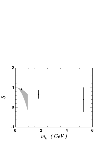
Figure 5: $\delta$ as a function of heavy-meson mass for fixed light meson mass $m_{L}=m_{\pi}$. The shaded band gives the prediction from CHPT valid for $m_{H}\lesssim 1\,{\rm GeV}$. Dots with error bars are experimental data as discussed in the text.

For $m_{H},m_{L}\ll\Lambda_{\rm QCD}$, the form factors can be expanded in powers of the small ratios of masses and momenta relative to the QCD scale (since the energies involved in semileptonic transitions are bounded by meson masses). In this regime of Chiral Perturbation Theory (CHPT) Gasser:1983yg ; Gasser:1984gg , $1-\delta$ is of order $m^{2}/\Lambda_{\rm QCD}^{2}$. The leading contribution is given by

$$\delta(m_{L},m_{H})$$

$$\quad=1-{2(m_{H}^{2}-m_{L}^{2})\over F_{0}^{2}}\big{[}L_{9}^{r}(\mu)-2L_{5}^{r}(\mu)+\dots\big{]}\,,$$

$$\quad\big{[}m_{H},m_{L}\ll\Lambda\big{]}\,,$$ (17)

where the ellipsis denotes a known kinematic function which cancels the renormalization-scale dependence of the low-energy constants $L_{5,9}^{r}(\mu)$. Here $F_{0}\propto f_{\pi}$ is related to the pion decay constant. The deviation of $\delta$ from unity is predicted by the sign of the combination $L_{9}^{r}-2L_{5}^{r}$, which is empirically found to be positive. The band in Fig 5 shows the allowed range of $\delta$, where for illustration we take Gasser:1984gg $F_{0}=0.088\,{\rm GeV}$, $10^{3}L_{5}^{r}(m_{\eta})=2.2\pm 0.5$ (determined from the ratio $f_{K}/f_{\pi}$) and $10^{3}L_{9}^{r}(m_{\eta})=7.4\pm 0.7$ (determined from the electromagnetic charge radius of the pion). The value of $\delta$ for $K^{0}\to\pi^{+}$ is taken from Alexopoulos:2004sy . The data point for $D\to\pi$ is discussed in Section VI, and the data point for $B\to\pi$ is the same as in Fig. 4.

IV.3 $m_{H}\gg\Lambda\gtrsim m_{L}$: SCET

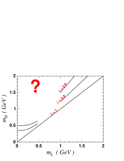
Figure 6: Contours of constant $\delta$ in the $m_{L}-m_{H}$ plane.

The HQET description in Section IV.1 breaks down when the light meson becomes light (Fig. 4). Similarly, the CHPT in Section IV.2 breaks down when the heavy meson becomes heavy (Fig. 5).

In this regime, since we are concerned with the point at maximum recoil, the light-meson energy necessarily satisfies $E\sim m_{H}/2\gg\Lambda_{\rm QCD}$. Observables can thus be analyzed using a simultaneous expansion in $\Lambda/m_{H}$ and $\Lambda/E$. The soft-collinear effective theory (SCET) framework has been developed to study this regime Bauer:2000ew ; Bauer:2000yr ; Chay:2002vy ; Beneke:2002ph ; Hill:2002vw . The leading description of the form factors for pseudoscalar-pseudoscalar transitions is, up to corrections of order $\alpha_{s}(m_{H})$ and $\Lambda/m_{H}\sim\Lambda/E$, Charles:1998dr ; Beneke:2000wa ; Bauer:2002aj ; Beneke:2003pa ; Lange:2003pk ; Hill:2004if ; Hill:2005ju

$$F_{+}(E) = \sqrt{m_{H}}\big{[}\zeta(E)+\left({4E\over m_{H}}-1\right)H(E)\big{]}\,,$$

$${m_{H}\over 2E}F_{0}(E) = \sqrt{m_{H}}\big{[}\zeta(E)+H(E)\big{]}\,,$$ (18)

where it is more natural to work here in terms of the light-meson energy, related to the invariant momentum transfer $t$ in (II) by $t=m_{H}^{2}+m_{L}^{2}-2m_{H}E$. The construction of SCET is more intricate than either HQET or CHPT, due to the nonfactorization of large and small momentum modes in some processes Becher:2003qh ; Becher:2003kh .  Apart from scaling violations related to this phenomenon, the functions $\zeta$ and $H$ both have an energy dependence $\zeta\sim H\sim E^{-2}$.

From expression (IV.3) it is straightforward to see that, independent of any model assumptions, Hill:2005ju

$${1\over\beta}=-\left.{d\ln(\zeta+H)\over d\ln E}\right|_{E=m_{H}/2}-1+{\cal O}(\alpha_{s},\Lambda/m_{H})\,.$$ (19)

From the $1/E^{2}$ asymptotic behavior of $\zeta$ and $H$, $1/\beta$ should approach unity as $m_{H}\to\infty$ at fixed $m_{L}\lesssim\Lambda_{\rm QCD}$. Similarly,

$$\delta(m_{L},m_{H}) = \left.{2H\over\zeta+H}\right|_{E=m_{H}/2}+{\cal O}(\alpha_{s},\Lambda/m_{H})\,,$$ (20)

$$\quad\big{[}m_{H}\gg\Lambda\gtrsim m_{L}\big{]}\,.$$

Thus the question of the asymptotic limit, $\lim_{m_{H}\to\infty}\delta(m_{L},m_{H})$, is the same as the question of which contribution, the “hard” function $H$, or the “soft” function $\zeta$, dominates in this limit.

The results summarized by (16), (IV.2) and (20), can be unified as in Fig. 6, which displays three equal-$\delta$ contours in the HQET and CHPT regimes. The obvious question is: what happens to these contours as we pass outside of these regimes? We know that $\delta$ cannot depend strongly on $m_{H}$, since this dependence is due solely to scaling violations and power corrections. A smooth chiral limit of the form factors also implies that $\delta$ cannot depend strongly on $m_{L}$. To further constrain these contours, experimental data can be used as a quantitative probe in this regime.

V Implications for phenomenology

We focus attention on the prototypical heavy-light process, $B\to\pi\ell\nu$. The methodology described in Section II can be used to extract as much information from experimental and lattice data as possible, with believable error estimates.

V.1 Precision measurements: $V_{ub}$

\psfrag{q}[T]{$t$ (${\rm GeV}^{2}$) }\psfrag{y}[B]{$10^{3}|V_{ub}|$}\includegraphics[width=227.62204pt]{q2valAAlt.eps}

Figure 7: Experimental error on $|V_{ub}|$, with theoretical input of the form factor normalization at a given value of $t$, from Becher:2005bg . The plot assumes that the fit yields the central value $|V_{ub}|=3.7\times 10^{-3}$.

Knowing that the true form factor is given by one of the restricted class of curves in (4) allows for maximal use of the available experimental  and lattice  data. Figure 7 shows the minimum error obtainable for $|V_{ub}|$ using present data Athar:2003yg ; Abe:2004zm ; Aubert:2005cd ; Aubert:2005tm , with a form factor determination at a given value of $t$ Becher:2005bg . The dark, medium and light bands correspond to increasing levels of conservatism for the size of the coefficients appearing in (4): $\sum_{k}a_{k}^{2}=0.01,0.1,1$, normalized relative to the default unitarity bound. At the point $t_{0}=16\,{\rm GeV}^{2}$, these values correspond to $\sum_{k}a_{k}^{2}/a_{0}^{2}\approx 25,250,2500$.

As Fig. 7 illustrates, theory inputs at either very large or very small $t$ are not as effective as for moderate values, say $t=10-20\,{\rm GeV}^{2}$, which are within the range currently studied with unquenched lattice simulations Okamoto:2004xg ; Shigemitsu:2004ft ; Gulez:2006dt . For extreme values of the bounds, e.g., allowing coefficients in the expansion (4) to be as large as $a_{k}/a_{0}\sim 50$, the error begins to increase, as the lighter bands in the figure show.

For consistency, the heavy-quark power counting used to establish bounds on the form factor shape should be at least as robust and conservative as similar estimates used to bound other theoretical errors entering a $|V_{ub}|$ determination—e.g. power corrections, perturbative matching corrections, or discretization errors in lattice calculations of the form factor. Quantitative investigations such as in Table 2 and Section VI give us confidence that as far as the bounds are concerned, “order unity” really means order unity.

V.2 Inputs to hadronic $B$ decays

Semileptonic decays provide a robust value for the form factor normalization (times $|V_{ub}|$), a key input to factorization analyses of two-body hadronic decays Bauer:1986bm ; Bjorken:1988kk ; Beneke:1999br ; Beneke:2000ry . From Becher:2005bg , 

$$10^{3}|V_{ub}F_{+}(0)|=0.92\pm 0.11\pm 0.03\,.$$ (21)

A dominant uncertainty in many factorization predictions is the normalization of the hard-scattering contribution to the form factor, commonly expressed in terms of an (inverse) moment of the $B$ meson wavefunction, $\lambda_{B}$:

$$\delta(m_{\pi},m_{B})={6\pi C_{F}\over N_{c}}{f_{B}f_{\pi}\alpha_{s}\over m_{B}\lambda_{B}F_{+}(0)}+\dots\,.$$ (22)

For example, the “default scenario” inputs of Beneke:2003zv give $\delta\approx 0.15^{+0.10}_{-0.05}$, while the “S2 scenario” gives a central value $\delta\approx 0.29$.  The semileptonic data can help pin down this number. From Becher:2005bg , using experimental data for $F_{+}$ from Athar:2003yg ; Abe:2004zm ; Aubert:2005cd ; Aubert:2005tm determines

$$B\to\pi:\quad\quad\quad$$

$$1+1/\beta-\delta = 1.5\pm 0.6\pm 0.4\,,$$ (23)

and the lattice value $\beta=1.2\pm 0.1$ from Shigemitsu:2004ft ; Okamoto:2004xg allows extraction of $\delta$.

If $\delta$ is monotonic as a function of $m_{L}$, the analysis of Section IV.1 shows that

$$\delta(m_{L},m_{B})<0.35\pm 0.03\,,\big{[}m_{L}<1\,{\rm GeV};{\rm monotonicity}\big{]}\,.$$ (24)

A significantly larger value of $\delta$, e.g. $\delta\sim 1$ Bauer:2004tj ; Bauer:2005kd ; Williamson:2006hb , would require a dramatic behavior of the extrapolated curve in Fig. 4.

VI What’s charm got to do with it?

Charm decays provide a direct probe of the “interesting” regime pictured in Fig. 6. They provide an important test of lattice measurements for heavy-to-light form factors, and a quantitative test of the power-counting used to bound the form factor shape in other processes such as $B\to\pi$.

VI.1 Fundamental questions

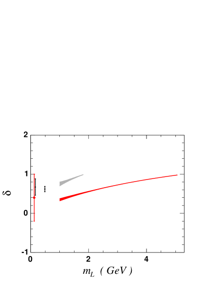
Figure 8: $\delta$ as a function of light-meson mass. The upper (black) points are for fixed $m_{H}=m_{D}$, and the lower (red) points for fixed $m_{H}=m_{B}$.

Depending on whether the soft or hard component of the form factor dominates in the limit $m_{H}\to\infty$, the difference in form factor slopes (IV) tends to $\delta\to 0$ or $\delta\to 2$. The latter would require that the curves such as in Fig. 4 turn upward at small $m_{L}$, for sufficiently large $m_{H}$. If this happens, and unless a new large scale is dynamically generated by QCD, at which a turnaround in the curves would occur, some evidence for this behavior should be evident in the charm system. Precision measurements here directly probe the dangerous region illustrated in Fig 6. For $D\to K$ decays,

$$D\to K:\quad\quad\quad$$

$$1+1/\beta-\delta = 1.03\pm 0.09\pm 0.11\quad\text{\cite[cite]{\@@bibref{Authors Phrase1YearPhrase2}{Huang:2004fr}{\@@citephrase{(}}{\@@citephrase{)}}}}$$ (25)

$$0.94\pm 0.07\pm 0.10\quad\text{\cite[cite]{\@@bibref{Authors Phrase1YearPhrase2}{Link:2004dh}{\@@citephrase{(}}{\@@citephrase{)}}}}$$

$$1.13\pm 0.10\pm 0.12\quad\text{\cite[cite]{\@@bibref{Authors Phrase1YearPhrase2}{Abe:2005sh}{\@@citephrase{(}}{\@@citephrase{)}}}}\,.$$

Here the first error is experimental using the linear $z$ parameterization (just $a_{0}$, $a_{1}$) in (4). The second error is a conservative estimate of the residual shape uncertainty, obtained by allowing an extra parameter in the fit ($a_{0}$, $a_{1}$ and $a_{2}$), with $|a_{k}/a_{0}|\lesssim 10$. Combining this with the lattice value $\beta=1.8\pm 0.1$ yields the $D\to K$ data point in Fig. 8.

Similarly for $D\to\pi$ decays,

$$D\to\pi:\quad\quad\quad$$

$$1+1/\beta-\delta = 1.3\pm 0.4\pm 0.5\quad\text{\cite[cite]{\@@bibref{Authors Phrase1YearPhrase2}{Huang:2004fr}{\@@citephrase{(}}{\@@citephrase{)}}}}$$ (26)

$$0.9\pm 0.2\pm 0.3\quad\text{\cite[cite]{\@@bibref{Authors Phrase1YearPhrase2}{Abe:2005sh}{\@@citephrase{(}}{\@@citephrase{)}}}}\,,$$

with the errors as above. Combined with the lattice value $\beta=1.65\pm 0.10$ yields the $D\to\pi$ data point in Fig. 5 and Fig. 8.

Our current combined knowledge of form factor shape from $B$ and $D$ decays is illustrated in Fig. 8. So far the data do not indicate surprises in either of the curves when extrapolated into the region $m_{L}\lesssim 1\,{\rm GeV}$. It will be interesting to probe this region with more precision when further data becomes available.

VI.2 Lattice, experiment and parameterizations

Charm decays provide important tests of nonperturbative methods used to evaluate hadronic matrix elements. When comparing the results of lattice QCD with experiment, it should be kept in mind that the kinematic regions that are studied with best precision are different for the lattice (large $t$) and experiment (small $t$). Also, the manner in which chiral extrapolations are performed to reach physical light-quark masses imply that it is difficult to present lattice results in terms of uncorrelated values of the form factor at different $t$ values. In practice, the results are generally presented in terms of a parameterized curve; to make a definitive comparison to experiment, it is essential that the chosen parameterization doesn’t introduce a bias. The ideas described in Section II allow a systematic approach to this problem mackenzie . The remainder of this subsection points out pitfalls that can occur with some of the simplified parameterizations in common use.

The starting point for many parameterizations is a more pedestrian but rigorous approach to analyticity, which implies the dispersion relation:

$$F_{+}(t)={F_{+}(0)\over 1-\alpha}{1\over 1-t/m_{H^{*}}^{2}}+{1\over\pi}\int_{t_{+}}^{\infty}{dt^{\prime}}{{\rm Im}F(t^{\prime})\over t^{\prime}-t}\,,$$ (27)

where a distinct $m_{H^{*}}$ pole appears below threshold for heavy-to-light decays such as $B\to\pi$ and $D\to K$ (and almost for $D\to\pi$). The first interesting test is to see whether just the $m_{H^{*}}$ pole can describe the data,

$$\begin{array}[]{ll}{\rm vector\,\,dominance}:\\ &\displaystyle{F_{+}(t)={F_{+}(0)\over 1-t/m_{H^{*}}^{2}}}\,.\quad\quad\quad\quad\quad\hskip 142.26378pt\phantom{a}\\ \end{array}$$ (28)

In fact this “vector dominance” model can be explicitly ruled out by the data Link:2004dh ; Huang:2004fr ; Abe:2005sh ; Abe:2005sh ; Athar:2003yg ; Aubert:2005cd ; Abe:2004zm , so that inclusion of the continuum contribution in (27) is essential.

From a dynamical point of view, in order to obtain the $1/E^{2}$ dependence appearing in heavy-to-light form factors, as in (IV.3), it is necessary that the continuum integral in (27) play a significant role. This can be treated in a model independent way by breaking up the integral into a sum of effective poles, and using power-counting estimates to establish reasonable bounds on the coefficients of these effective poles Hill:2005ju ; Becher:2005bg . In the first approximation, the continuum integral is represented by a single effective pole, and two parameters are necessary to describe its location and strength relative to the $H^{*}$ pole. Since this is one more parameter than is easily measured from the data, various suggestions have been made for eliminating one of these parameters.

The “single pole model”, where both the $H^{*}$ pole and the continuum integral are represented by a single pole that is allowed to float,

$$\begin{array}[]{ll}{\rm single\,\,pole}:\\ &\displaystyle{F_{+}(t)={F_{+}(0)\over 1-t/m_{\rm pole}^{2}}}\,,\\ \end{array}$$ (29)

is also ruled out by the data, although in a slightly less direct way. Although the curve can be made to fit, the pole position is forced to take an unphysical value, significantly below both the $H^{*}$ pole and the continuum. The “modified pole model”,

$$\begin{array}[]{ll}{\rm modified\,\,pole}:\\ &\displaystyle{F_{+}(t)={F_{+}(0)\over\left(1-t/m_{H^{*}}^{2}\right)\left(1-\alpha_{\rm pole}t/m_{H^{*}}^{2}\right)}}\,,\end{array}$$ (30)

holds a similar status. For $D\to K$ and $D\to\pi$, (VI.1) and (VI.1) clearly show that $1+1/\beta-\delta\approx 2$ is not valid for charm decays, as necessary for the motivation for the simplification (30) proposed in Becirevic:1999kt . Although the form (30) can be made to fit the data, there is no obvious physical interpretation for the resulting fit parameter; in particular $\alpha_{\rm pole}$ obtained in this way has no direct relation to the physical $\alpha$ defined in (27).

It should be kept in mind that unless there is a physical meaning that can be given to the parameter being studied, there is no guarantee that different experimental or lattice determinations will converge to any one value for this parameter. It is therefore unclear what to make of discrepancies appearing when different datasets are forced to fit models such as (29) or (30) Wiss:2006ih ; poling . The situation is especially dangerous for comparing lattice and experiment, since the range of $t$ that is emphasized is different in the two cases. These pitfalls are easily avoided by working with a general parameterization such as (4) that is guaranteed to contain the true form factor, and by comparing physical quantities, such as in (VI.1), (VI.1).

VI.3 Testing convergence

The general parameterization (4) provides a systematic procedure for estimating how many terms should be resolved by data at a given level of precision. Rigorous bounds are placed on the coefficients by using crossing symmetry to analyze the production form factor, either via unitarity arguments, or through power counting of contributions from different momentum regions. Since the latter estimates yield constraints that are so much more powerful than can be safely estimated by unitarity, it is important to check wherever possible that large “order unity” numbers don’t appear. As illustrated by Table 2, the available semileptonic data reveal no surprises.

VII Decays of pseudoscalar to vector mesons

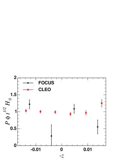
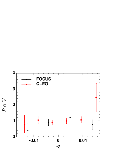
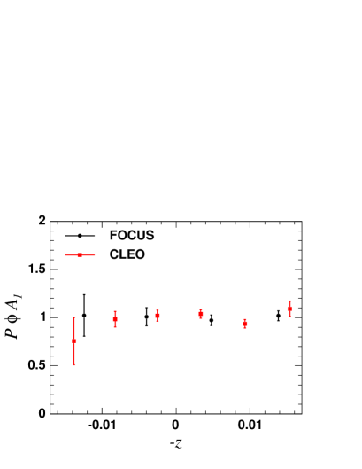
Figure 9: Experimental data for helicity amplitudes in $D\to K^{*}\ell\nu$, from Link:2005dp ; Shepherd:2006tw . Units on the vertical axis are arbitrary (approximately normalized to unity at $t=0$).

Pseudoscalar-pseudoscalar transitions hold a priveleged position, from a first-principles simplicity point of view, from the lattice point of view, and from the experimental point of view. Pseudoscalar-vector transitions, while accompanied by new complications, are however important backgrounds to the pseudosclar mode, provide alternative extractions of CKM parameters, and yield important constraints on radiative and hadronic transitions. This section briefly outlines the implementation of the ideas in Section II to the pseudoscalar-vector case. 

The most obvious complication is the multiple invariant form factors that accompany the vector particle. Less obvious complications involve modifications to the analytic structure of the form factors due to the unstable nature of vector mesons, and the possible existence of anomalous thresholds. When these occur, they will encroach on the gap between the semileptonic region and singularities. The effects of such anomalous thresholds are not expected to be large, and can be investigated on a case-by-case basis.  A more complete discussion is beyond the scope of this talk and we ignore such complications here.

Table 3: Maximum $|z(t,t_{0})|$ throughout semileptonic range with symmetrizing choice $t_{0}=t_{+}(1-\sqrt{1-t_{-}/t_{+}})$.

Process	$|z|_{\rm max}$
$D\to K^{*}$	0.017
$D\to\rho$	0.024
$B\to D^{*}$	0.028
$B\to\rho$	0.10

In heavy-to-heavy decays it is possible to relate form factors by heavy-quark symmetry, making the pseudoscalar-vector analysis not significantly different, from the point of view of the number of independent invariant form factors, from the pseudoscalar-pseudoscalar case. For heavy-to-light decays, this simplification is not possible; however, a new symmetry emerges due to the large energy of the vector meson, and the resulting suppression of the helicity-flip amplitude Burdman:2000ku ; Beneke:2000wa ; Hill:2004if . It is again important to take advantage of as much first-principles knowledge as possible. By the same variable transformation (3), the invariant form factors may all be written in terms of a convergent expansion in a small parameter governed by the degree of isolation of the semileptonic region. Table 3 shows the maximum size of the parameter when $t_{0}=t_{+}(1-\sqrt{1-t_{-}/t_{+}})$, for processes involving ground state heavy-light pseudoscalar mesons decaying into the lowest-lying vector mesons.

The decay rate can be decomposed in terms of helicity amplitudes Korner:1989qb , 

$${\sqrt{t}H_{0}\over m_{H}^{2}} = {(1+\hat{m_{L}})^{2}(\hat{E}_{L}-\hat{m_{L}}^{2})A_{1}-2\hat{k}_{L}^{2}A_{2}\over\hat{m}_{L}(1+\hat{m}_{L})}\,,$$

$${H_{\pm}\over m_{H}} = {(1+\hat{m}_{L})^{2}A_{1}\mp 2\hat{k}_{L}V\over 1+\hat{m}_{L}}\,,$$ (31)

where hatted variables are in units of $m_{H}$, and $E_{L}$ and $k_{L}$ denote the energy and momentum of the light vector meson in the rest frame of the heavy pseudoscalar meson. The amplitudes $\sqrt{t}H_{0}$, $V$ and $A_{1}$ correspond to cross-channel production of states with quantum numbers $J^{P}=1^{+}$, $1^{-}$ and $1^{+}$, respectively. On the premise of analyticity, these functions can be expanded as in (4). For the choice of $\phi$, we use the form motivated by unitarity (although the evaluation of the unitarity bound itself is not directly relevant). Using the results of Caprini:1997mu , at $Q=0$,

$$\phi_{\sqrt{t}H_{0}}(t,t_{0}) \propto {\sqrt{t_{+}-t}\over(t_{+}-t_{0})^{1/4}}\left(z(t,0)\over-t\right)^{5/2}\left(z(t,t_{0})\over t_{0}-t\right)^{-1/2}$$

$$\times\left(z(t,t_{-})\over t_{-}-t\right)^{-1/4}\,,$$

$$\phi_{V}(t,t_{0}) \propto {t_{+}-t\over(t_{+}-t_{0})^{1/4}}\left(z(t,0)\over-t\right)^{5/2}\left(z(t,t_{0})\over t_{0}-t\right)^{-1/2}$$

$$\times\left(z(t,t_{-})\over t_{-}-t\right)^{-3/4}\,,$$

$$\phi_{A_{1}}(t,t_{0}) \propto {\sqrt{t_{+}-t}\over(t_{+}-t_{0})^{1/4}}\left(z(t,0)\over-t\right)^{2}\left(z(t,t_{0})\over t_{0}-t\right)^{-1/2}$$ (32)

$$\times\left(z(t,t_{-})\over t_{-}-t\right)^{-1/4}\,.$$

For the function $P$, we use for the resonances lying below threshold: DiPierro:2001uu ; Eichten:2005sf $J^{P}=1^{-}:m=2.11,2.63\,{\rm GeV}$; $J^{P}=1^{+}:m=2.46,2.56\,{\rm GeV}$. 

Fig. 9 shows the resulting invariant form factors extracted from the nonparametric analyses in Link:2005dp ; Shepherd:2006tw , after extracting the kinematic function $P\phi$, and transforming to the variable $z$. The small size of $z$ implies that these functions should deviate from a straight horizontal line by only a few percent over the entire range. With this in mind, it is straightforward to extract useful information in a systematic way. For instance, we can test the ${\cal O}(\Lambda_{\rm QCD}/m_{c})$ suppression of helicity amplitudes at $t=0$: [equivalently, measure the form factor ratio $V(0)/A_{1}(0)$]

$${H_{+}\over H_{-}} = 0.27\pm 0.06\quad\text{\cite[cite]{\@@bibref{Authors Phrase1YearPhrase2}{Link:2005dp}{\@@citephrase{(}}{\@@citephrase{)}}} }$$ (33)

$$0.37\pm 0.04\quad\text{\cite[cite]{\@@bibref{Authors Phrase1YearPhrase2}{Shepherd:2006tw}{\@@citephrase{(}}{\@@citephrase{)}}} }\,,$$

up to corrections of ${\cal O}(z)$.

VIII Summary

There is interesting information lurking in the semileptonic data, with applications to precision phenomenology, and for exploring a poorly-understood limit of QCD. As a practical matter, a simple and well-known variable transformation provides a powerful tool for analyzing and making full use of the semileptonic data. The effectiveness of this transformation has been obscured by a reliance on unitarity bounds, which were used as safe estimates in the absence of experimental data. Rigorous arguments for a stronger convergence of the expansion (4) are now available, and can be further tested and refined using experimental data from many semileptonic decay modes.

- (1) For reviews see e.g.: S. Eidelman et al. [Particle Data Group], Phys. Lett. B 592, 1 (2004). A. Hocker and Z. Ligeti, hep-ph/0605217.
- (2) A. J. Buras and L. Silvestrini, Nucl. Phys. B 569, 3 (2000) [hep-ph/9812392].
- (3) J. D. Bjorken and S. D. Drell, Relativistic Quantum Fields, McGraw-Hill, 1965.
- (4) C. Bourrely, B. Machet and E. de Rafael, Nucl. Phys. B 189, 157 (1981).
- (5) C. G. Boyd, B. Grinstein and R. F. Lebed, Phys. Rev. Lett. 74, 4603 (1995) [hep-ph/9412324].
- (6) L. Lellouch, Nucl. Phys. B 479, 353 (1996) [hep-ph/9509358].
- (7) C. G. Boyd, B. Grinstein and R. F. Lebed, Nucl. Phys. B 461, 493 (1996) [hep-ph/9508211].
- (8) I. Caprini and M. Neubert, Phys. Lett. B 380, 376 (1996) [hep-ph/9603414].
- (9) I. Caprini, L. Lellouch and M. Neubert, Nucl. Phys. B 530, 153 (1998) [hep-ph/9712417].
- (10) C. G. Boyd and M. J. Savage, Phys. Rev. D 56, 303 (1997) [hep-ph/9702300].
- (11) D. Weingarten, Phys. Rev. Lett. 51, 1830 (1983).
- (12) B. Aubert et al. [BABAR Collaboration], Phys. Rev. D 72, 051102 (2005) [hep-ex/0507003].
- (13) K. Abe et al. [Belle Collaboration], Phys. Lett. B 526, 258 (2002) [hep-ex/0111082].
- (14) O. P. Yushchenko et al., Phys. Lett. B 589, 111 (2004) [hep-ex/0404030].
- (15) T. Alexopoulos et al. [KTeV Collaboration], Phys. Rev. D 70, 092007 (2004) [hep-ex/0406003].
- (16) A. Lai et al. [NA48 Collaboration], Phys. Lett. B 604, 1 (2004) [hep-ex/0410065].
- (17) F. Ambrosino et al. [KLOE Collaboration], Phys. Lett. B 636, 166 (2006) [hep-ex/0601038].
- (18) G. S. Huang et al. [CLEO Collaboration], Phys. Rev. Lett. 94, 011802 (2005) [hep-ex/0407035].
- (19) J. M. Link et al. [FOCUS Collaboration], Phys. Lett. B 607, 233 (2005) [hep-ex/0410037].
- (20) K. Abe et al. [BELLE Collaboration], hep-ex/0510003.
- (21) S. B. Athar et al. [CLEO Collaboration], Phys. Rev. D 68, 072003 (2003) [hep-ex/0304019].
- (22) K. Abe et al. [BELLE Collaboration], hep-ex/0408145.
- (23) R. J. Hill, hep-ph/0607108.
- (24) E. J. Eichten and C. Quigg, Phys. Rev. D 49, 5845 (1994) [hep-ph/9402210].
- (25) V. Cirigliano, M. Knecht, H. Neufeld and H. Pichl, Eur. Phys. J. C 27, 255 (2003) [hep-ph/0209226].
- (26) M. Fukunaga and T. Onogi, Phys. Rev. D 71, 034506 (2005) [hep-lat/0408037].
- (27) M. C. Arnesen, B. Grinstein, I. Z. Rothstein and I. W. Stewart, Phys. Rev. Lett. 95, 071802 (2005) [hep-ph/0504209].
- (28) R. J. Hill, Phys. Rev. D 73, 014012 (2006) [hep-ph/0505129].
- (29) L. M. Chounet, J. M. Gaillard and M. K. Gillard, Phys. Rept. 4, 199 (1972).
- (30) S. S. Gershtein and M. Y. Khlopov, Pisma Zh. Eksp. Teor. Fiz. 23, 374 (1976). [English translation: JETP Lett.(1976) V.23, PP. 338-340]
- (31) M. Y. Khlopov, Yad. Fiz. I8, 1134 (1978). [English translation: Sov.J.Nucl.Phys. (1978) V. 28, no. 4, PP. 583-584].
- (32) R. Akhoury, G. Sterman and Y. P. Yao, Phys. Rev. D 50, 358 (1994).
- (33) N. Isgur and M. B. Wise, Phys. Lett. B 237, 527 (1990).
- (34) For a review see: M. Neubert, Phys. Rept. 245, 259 (1994) [hep-ph/9306320].
- (35) J. Gasser and H. Leutwyler, Annals Phys. 158, 142 (1984).
- (36) J. Gasser and H. Leutwyler, Nucl. Phys. B 250, 465 (1985).
- (37) C. W. Bauer, S. Fleming and M. E. Luke, Phys. Rev. D 63, 014006 (2001) [hep-ph/0005275].
- (38) C. W. Bauer, S. Fleming, D. Pirjol and I. W. Stewart, Phys. Rev. D 63, 114020 (2001) [hep-ph/0011336].
- (39) J. Chay and C. Kim, Phys. Rev. D 65, 114016 (2002) [hep-ph/0201197].
- (40) M. Beneke, A. P. Chapovsky, M. Diehl and T. Feldmann, Nucl. Phys. B 643, 431 (2002) [hep-ph/0206152].
- (41) R. J. Hill and M. Neubert, Nucl. Phys. B 657, 229 (2003) [hep-ph/0211018].
- (42) J. Charles, A. Le Yaouanc, L. Oliver, O. Pene and J. C. Raynal, Phys. Rev. D 60, 014001 (1999) [hep-ph/9812358].
- (43) M. Beneke and T. Feldmann, Nucl. Phys. B 592, 3 (2001) [hep-ph/0008255].
- (44) C. W. Bauer, D. Pirjol and I. W. Stewart, Phys. Rev. D 67, 071502 (2003) [hep-ph/0211069].
- (45) M. Beneke and T. Feldmann, Nucl. Phys. B 685, 249 (2004) [hep-ph/0311335].
- (46) B. O. Lange and M. Neubert, Nucl. Phys. B 690, 249 (2004) [Erratum-ibid. B 723, 201 (2005)] [hep-ph/0311345].
- (47) R. J. Hill, T. Becher, S. J. Lee and M. Neubert, JHEP 0407, 081 (2004) [hep-ph/0404217].
- (48) T. Becher, R. J. Hill and M. Neubert, Phys. Rev. D 69, 054017 (2004) [hep-ph/0308122].
- (49) T. Becher, R. J. Hill, B. O. Lange and M. Neubert, Phys. Rev. D 69, 034013 (2004) [hep-ph/0309227].
- (50) A. V. Manohar and I. W. Stewart, hep-ph/0605001.
- (51) K. Varvell, Talk at FPCP 2006, hep-ex/0605077.
- (52) B. Aubert et al. [BABAR Collaboration], hep-ex/0506064.
- (53) T. Becher and R. J. Hill, Phys. Lett. B 633, 61 (2006) [hep-ph/0509090].
- (54) M. Okamoto et al., Nucl. Phys. Proc. Suppl. 140, 461 (2005) [hep-lat/0409116].
- (55) J. Shigemitsu et al., Nucl. Phys. Proc. Suppl. 140, 464 (2005) [hep-lat/0408019].
- (56) E. Gulez, A. Gray, M. Wingate, C. T. H. Davies, G. P. Lepage and J. Shigemitsu, hep-lat/0601021.
- (57) M. Wingate, Mod. Phys. Lett. A 21, 1167 (2006) [hep-ph/0604254].
- (58) P. Mackenzie, Talk at FPCP 2006, hep-ph/0606034.
- (59) M. Bauer, B. Stech and M. Wirbel, Z. Phys. C 34, 103 (1987).
- (60) J. D. Bjorken, Nucl. Phys. Proc. Suppl. 11, 325 (1989).
- (61) M. Beneke, G. Buchalla, M. Neubert and C. T. Sachrajda, Phys. Rev. Lett. 83, 1914 (1999) [hep-ph/9905312].
- (62) M. Beneke, G. Buchalla, M. Neubert and C. T. Sachrajda, Nucl. Phys. B 591, 313 (2000) [hep-ph/0006124].
- (63) M. Beneke and M. Neubert, Nucl. Phys. B 675, 333 (2003) [hep-ph/0308039].
- (64) Z. Luo and J. L. Rosner, Phys. Rev. D 68, 074010 (2003) [hep-ph/0305262].
- (65) C. W. Bauer, D. Pirjol, I. Z. Rothstein and I. W. Stewart, Phys. Rev. D 70, 054015 (2004) [hep-ph/0401188].
- (66) C. W. Bauer, I. Z. Rothstein and I. W. Stewart, hep-ph/0510241.
- (67) A. R. Williamson and J. Zupan, hep-ph/0601214.
- (68) D. Becirevic and A. B. Kaidalov, Phys. Lett. B 478, 417 (2000) [hep-ph/9904490].
- (69) J. Wiss, Talk at FPCP 2006, hep-ex/0605030.
- (70) R. Poling, Talk at FPCP 2006, hep-ex/0606016.
- (71) S. Fajfer and J. Kamenik, Phys. Rev. D 72, 034029 (2005) [hep-ph/0506051].
- (72) S. Fajfer and J. Kamenik, Phys. Rev. D 73, 057503 (2006) [hep-ph/0601028].
- (73) D. Ebert, R. N. Faustov and V. O. Galkin, Phys. Rev. D 64, 094022 (2001) [hep-ph/0107065].
- (74) G. Burdman and G. Hiller, Phys. Rev. D 63, 113008 (2001) [hep-ph/0011266].
- (75) J. G. Korner and G. A. Schuler, Z. Phys. C 46, 93 (1990).
- (76) R. J. Hill, Nucl. Phys. Proc. Suppl. 152, 184 (2006) [hep-ph/0411073].
- (77) M. Di Pierro and E. Eichten, Phys. Rev. D 64, 114004 (2001) [hep-ph/0104208].
- (78) E. Eichten, Nucl. Phys. Proc. Suppl. 142, 242 (2005).
- (79) J. M. Link et al. [FOCUS Collaboration], Phys. Lett. B 633, 183 (2006) [hep-ex/0509027].
- (80) M. R. Shepherd et al. [CLEO Collaboration], “Model independent measurement of form factors in the decay D+ K- pi+ hep-ex/0606010.