The nature of $\sigma$, $\kappa$, $a_{0}(980)$ and $f_{0}(980)$

Abstract

Masses and widths of the four light scalar mesons $\sigma$, $\kappa$, $a_{0}$(980) and $f_{0}$(980) may be reproduced in a model where mesons scatter via a $q\bar{q}$ loop. A transition potential is used to couple mesons to $q\bar{q}$ at a radius of $\sim 0.57$ fm. Inside this radius, there is an infinite bare spectrum of confined $q\bar{q}$ states, for which a harmonic oscillator is chosen here. The coupled-channel system approximately reproduces the features of both light and heavy meson spectroscopy. The generation of $\sigma$, $\kappa$, $a_{0}(980)$ and $f_{0}(980)$ is a balance between attraction due to the $q\bar{q}$ loop and suppression of the amplitudes at the Adler zeros. Phase shifts increase more rapidly as the coupling constant to the mesons increases. This leads to resonant widths which decrease with increasing coupling constant — a characteristically non-perturbative effect.
PACS numbers: 14.40.Cs, 14.40.Ev, 13.25.-k, 13.75.Lb

Recent experiments have improved parameters of $\sigma$, $\kappa$, $a_{0}(980)$ and $f_{0}(980)$ [1]–[8], and there are now extensive data on their couplings to decay channels. Their masses do not conform to the pattern set by well-known $q\bar{q}$ nonets, e.g. $\rho$, $\omega$, $K^{*}(890)$ and $\phi$. The mass of the $a_{0}(980)$ is $\sim 450$ MeV above the mass of the $\sigma$, unlike the near degeneracy between $\rho$ and $\omega$. This has led Jaffe to suggest that they are 4-quark states [9]. However, Scadron has shown that the existence of a light scalar nonet may be a direct consequence of dynamical chiral-symmetry breaking [10].

Here, we present a simple model which reproduces their essential features. It fits $\pi\pi$ and $K\pi$ elastic phase shifts, and also the line-shapes of $a_{0}(980)$ and $f_{0}(980)$, i.e., $a_{0}\to\pi\eta$, $KK$ and $\pi\eta^{\prime}$, and $f_{0}\to\pi\pi$, $KK$ and $\eta\eta$.

The model in its two versions has been described in earlier publications [11][12]. In one formulation [11], an explicit harmonic oscillator potential, with corresponding wave functions, is used for the bare $q\bar{q}$ states; it reproduces the gross features of the spectra of both light and heavy mesons. In the other approach [12], use is made of a so-called Resonance Spectrum Expansion, which allows, in principle, the use of any confinement spectrum for the bare states. In the present paper, the latter method is applied, though again with a harmonic oscillator. This choice is not crucial, as e.g. the $f_{0}(1370)$ lies well above states considered here and couples mostly to $4\pi$. So the more conventional funnel potential is expected to give similar results.

The confining potential is joined at radius $r_{0}$ to plane waves for meson pairs. Decays of $q\bar{q}$ states trapped in the confining potential are described by Fig. 1.

     

Figure 1: Schematic picture of the model.

The $\sigma$, $\kappa$, $f_{0}(980)$ and $a_{0}(980)$ appear as extra states through their dynamical coupling to this $q\bar{q}$ loop. If it were not for this coupling, they would be plane waves in the continuum. Coupling of mesons to the loops induces some degree of mixing of regular $q\bar{q}$ states with $\sigma$ and its relatives.

A universal coupling constant $\lambda$ is used for quarks of all flavours, after a mass scaling as a function of the reduced quark mass ensuring approximate flavour blindness of our equations, provided the same scaling is applied to the radius $r_{0}$ [13]. The relative 3-meson couplings at each vertex are taken from Tables I and II of Anisovich et al. [14]. These are the usual $SU(3)$-symmetric couplings for OZI-allowed decays, to be contrasted with the totally flavour-symmetric choice used in the second paper of Ref. [11]. The latter convention gives rise to equally good fits, but results in a significantly larger value of $\lambda$ for the coupled $\sigma$-$f_{0}$(980), as compared to the $\kappa$ and $a_{0}$(980), in the present restriction to pseudoscalar-pseudoscalar (PP) decay channels only. The formulae allow for the pseudoscalar mixing angle $\Theta_{PS}$ in the couplings of $\eta$ and $\eta^{\prime}$,

$$\begin{array}[]{r}\eta\;=\;n\bar{n}\cos(\Theta_{0}+\Theta_{PS})-s\bar{s}\sin(\Theta_{0}+\Theta_{PS})\;,\\[2.84526pt] \eta^{\prime}\;=\;n\bar{n}\sin(\Theta_{0}+\Theta_{PS})+s\bar{s}\cos(\Theta_{0}+\Theta_{PS})\;,\end{array}$$ (1)

where $\Theta_{0}=\arctan\sqrt{2}\approx 54.7^{\circ}$, thus defining $\Theta_{PS}$ in the octet-singlet basis. The intrinsic (or bare) mixing between $\sigma$ and $f_{0}(980)$ is likewise expressed, this time in the $n\bar{n}$-$s\bar{s}$ basis, in terms of a scalar mixing angle $\Theta_{S}$ by

$$\begin{array}[]{r}\sigma\;=\;n\bar{n}\cos\Theta_{S}-s\bar{s}\sin\Theta_{S}\;,\\[2.84526pt] f_{0}\;=\;n\bar{n}\sin\Theta_{S}+s\bar{s}\cos\Theta_{S}\;.\end{array}$$ (2)

Coupled relativistic Schrödinger equations are solved outside and inside the radius $r_{0}$, and are matched at that radius. The resulting multichannel $T$ matrix can be written down in closed form. In the case of the $\kappa$ and the $a_{0}$(980), as well as the decoupled $\sigma$ and $f_{0}$(980), there is only one $q\bar{q}$ channel, resulting in the relatively simple expression

$$T_{ij}(E)\;=\;-\frac{\displaystyle 2r_{0}\lambda^{2}\left\{\sum_{s=0}^{\infty}\frac{g_{i}(s)g_{j}(s)}{E-E_{s}}\right\}\sqrt{\mu_{i}\mu_{j}k_{i}k_{j}}\,j_{\ell_{i}}(k_{i}r_{0})\,j_{\ell_{j}}(k_{j}r_{0})}{\displaystyle 1\,+\,2ir_{0}\lambda^{2}\sum_{n=1}^{N_{f}}\left\{\sum_{s=0}^{\infty}\frac{g_{n}^{2}(s)}{E-E_{s}}\right\}\mu_{n}k_{n}\,j_{\ell_{n}}(k_{n}r_{0})\,h^{(1)}_{\ell_{n}}(k_{n}r_{0})}\;,$$ (3)

where $\lambda$ is the overall coupling, $r_{0}$ is the delta-shell radius, $g_{i}(s)$ is the relative coupling of the $i$th ($i=1,N_{f}$) two-meson channel, depending on the radial excitation (see Ref. [12], Table 1 of 4th paper), $E_{s}$ are the levels of the discrete confinement spectrum, $\mu_{i}=\mu_{i}(E)$ and $k_{i}=k_{i}(E)$ are the relativistic reduced mass and momentum in the $i$th channel, and $j_{\ell_{i}}$ and $h^{(1)}_{\ell_{i}}$ are spherical Bessel and Hankel functions, respectively. For the coupled $\sigma$ and $f_{0}$(980), there are two $q\bar{q}$ channels, i.e., $n\bar{n}$ and $s\bar{s}$, giving rise to a more complicated expression. Writing $T_{ij}(E)=N_{ij}(E)/D(E)$, we have

$$N_{ij}(E)\;=\;-2r_{0}\lambda^{2}\sqrt{\mu_{i}\mu_{j}k_{i}k_{j}}\,j_{\ell_{i}}(k_{i}r_{0})\,j_{\ell_{j}}(k_{j}r_{0})\left(\rule{0.0pt}{28.45274pt}\sum_{\alpha=1}^{2}\left\{\sum_{s=0}^{\infty}\frac{g_{\alpha i}(s)g_{\alpha j}(s)}{E-E_{\alpha s}}\right\}\right.\;+\;$$ (4)

$$+ \left.2ir_{0}\lambda^{2}\sum_{n=1}^{N_{f}}\left\{\sum_{s,s^{\prime}=0}^{\infty}\raisebox{-5.69054pt}{$\frac{\displaystyle\left|\begin{array}[]{cc}g_{1i}(s)&g_{1n}(s)\\ g_{2i}(s^{\prime})&g_{2n}(s^{\prime})\end{array}\right|\left|\begin{array}[]{cc}g_{1j}(s)&g_{1n}(s)\\ g_{2j}(s^{\prime})&g_{2n}(s^{\prime})\end{array}\right|}{\displaystyle\rule{0.0pt}{14.22636pt}(E-E_{1s})(E-E_{2s^{\prime}})}$}\right\}\mu_{n}k_{n}\,j_{\ell_{n}}(k_{n}r_{0})\,h^{(1)}_{\ell_{n}}(k_{n}r_{0})\right)$$ (9)

and

$$D(E)\;=\;1+2ir_{0}\lambda^{2}\sum_{\alpha=1}^{2}\sum_{n=1}^{N_{f}}\left\{\sum_{s=0}^{\infty}\frac{g^{2}_{\alpha n}(s)}{E-E_{\alpha s}}\right\}\mu_{n}k_{n}\,j_{\ell_{n}}(k_{n}r_{0})\,h^{(1)}_{\ell_{n}}(k_{n}r_{0})\;+\;$$ (10)

$$\!\!-\!\! 2r^{2}_{0}\lambda^{4}\!\!\sum_{\stackrel{{\scriptstyle\scriptstyle n,n^{\prime}=1}}{{n\neq n^{\prime}}}}^{N_{f}}\left\{\sum_{s,s^{\prime}=0}^{\infty}\raisebox{-5.69054pt}{$\frac{\displaystyle\left|\begin{array}[]{cc}g_{1n}(s)&g_{1n^{\prime}}(s)\\ g_{2n}(s^{\prime})&g_{2n^{\prime}}(s^{\prime})\end{array}\right|^{2}}{\displaystyle\rule{0.0pt}{14.22636pt}(E-E_{1s})(E-E_{2s^{\prime}})}$}\right\}\mu_{n}k_{n}\,j_{\ell_{n}}(k_{n}r_{0})\,h^{(1)}_{\ell_{n}}(k_{n}r_{0})\,\mu_{n^{\prime}}k_{n^{\prime}}\,j_{\ell_{n^{\prime}}}(k_{n^{\prime}}r_{0})\,h^{(1)}_{\ell_{n^{\prime}}}(k_{n^{\prime}}r_{0})\;,$$ (13)

where the index $\alpha=1,2$ refers to the $n\bar{n}$ and $s\bar{s}$ confinement channels, respectively.

The formulae of Anisovich et al. allow for separate coupling constants for $s\bar{s}$ and $n\bar{n}$; we find this refinement does not give any significant improvement, so we use the same value of $\lambda$ for both.

A key feature of the model lies in the automatic inclusion of Adler zeros in scattering amplitudes, which results from using relativistic reduced masses for two-meson channels [15]. It leads to Adler zeros at $s=0$ for $\pi\pi$ and $KK$, at $s=m^{2}_{\eta}-m^{2}_{\pi}$ for $\eta\pi$, and at $s=m^{2}_{K}-m^{2}_{\pi}$ for $K\pi$; although these are not quite conventional values, e.g. $0.5\,m^{2}_{\pi}$ for $\pi\pi$, the difference is insignificant for present purposes. The Adler zeros are essential to reproduce $\pi\pi$ and $K\pi$ elastic phase shifts near threshold [16].

Experimental data are used to determine the coupling constant $\lambda$ and transition radius $r_{0}$. The optimum values turn out to be in rough agreement with those in previous work [12][13] (see below). Phase shifts for $\pi\pi\to\pi\pi$ are taken from the BES publication [2] on the $\sigma$ pole (Method 1), where a combined fit was made to (i) BES data on $J/\Psi\to\omega\pi^{+}\pi^{-}$; (ii) Cern-Munich data [17]; (iii) $K_{e4}$ data of Pislak et al. [18]; (iv) the $\pi\pi$ scattering length $a_{0}=0.220\pm 0.005$ determined from chiral perturbation theory (ChPT) by Colangelo, Gasser and Leutwyler [19]. Phase shifts for $K\pi\to K\pi$ are taken from the combined fit [7] to LASS data for $K\pi$ elastic scattering [20], and E791 [4] and BES data [5][6] for the $\kappa$ pole; because of uncertainties in fitting $K_{0}^{*}(1430)$ (discussed below), the fit is made from threshold to 1.2 GeV after subtracting phases due to $K_{0}^{*}(1430)$. The line-shape of $a_{0}(980)$ is taken from the recent combined analysis [21] of KLOE data for $\phi\to\gamma a_{0}$ [22], and Crystal Barrel data on $\bar{p}p\to\omega a_{0}$ and $a_{0}\pi$ [23]. The line-shape of $f_{0}(980)$ is taken from BES data [8].

The coupling constant $\lambda$ and radius $r_{0}$ are fitted for each scalar resonance separately, except for the $f_{0}(980)$. We also make a combined fit to $\sigma$ + $f_{0}(980)$, in which both states emerge dynamically, by coupling the bare isoscalar $n\bar{n}$ and $s\bar{s}$ channels to $\pi\pi$, $KK$, $\eta\eta$, $\eta\eta^{\prime}$ and $\eta^{\prime}\eta^{\prime}$. Note that, although there is no direct coupling of $s\bar{s}$ to $\pi\pi$, the higher-order OZI-allowed process $s\bar{s}\to KK\to n\bar{n}\to\pi\pi$ does produce a coupling after all. This also produces a dynamical mixing of $n\bar{n}$ and $s\bar{s}$, in addition to the intrinsic quark-level mixing assumed above. Results for parameters and pole positions are shown in Table 1.

Resonance	$\lambda$	$r_{0}$	Pole Positions
	(GeV-3/2)	(GeV-1)	(MeV)
$\sigma$	2.92	2.84	555 - i262
$\kappa$	2.97	3.29	745 - i316
$a_{0}(980)$	2.62	2.81	1021 - i47
$\sigma+f_{0}(980)$	3.11	2.71	530 - i226 , 1007 - i38

Table 1: Fitted parameters. For $a_{0}$ and $f_{0}$, second-sheet poles are quoted.

Striking is the considerable effect on the $\sigma$ pole from coupling to the $f_{0}$(980), showing the influence of $n\bar{n}$-$s\bar{s}$ mixing via the kaon loop. As for the parameters, there is a reasonable agreement for all cases. The $\lambda$ parameter varies by $\pm 9\%$ and the radius parameter by $\pm 10\%$. Moreover, both parameters are roughly compatible with the values $\lambda=0.75$ GeV^-3/2 and $r_{0}=3.2$ GeV^-1 used in previous model calculations with only one continuum channel [12][13], taking into account that in the present study the squared relative couplings of the included PP channels are normalised so as to add up to 1/16, whereas in the single-channel case this number was just set to 1. Some small variations of parameters are to be expected due to the choice of a delta shell for the transition potential, which is very sensitive to the precise radial wave functions of the different PP channels. We shall comment on global features first and return to detail later.

Figure 2: Fits to (a) the $\sigma$ component of the $\pi\pi$ phase shift for elastic scattering; (b) the $\kappa$ component of $K\pi$ phase shifts for elastic scattering; (c) + (d) the line shapes of $f_{0}(980)$ and $a_{0}(980)$ in $\pi\pi$ resp. $\pi\eta$ channels.

In Fig. 2(a), the dashed curve shows our fit to the BES fit (full curve) to $\pi\pi$ phase shifts after subtracting the $f_{0}(980)$ component. Structure in our fit near the $KK$ and $\eta\eta$ thresholds originates from $\sigma\to KK$ and $\eta\eta$. These thresholds were not included in the analysis of BES data, so the comparison illustrates the magnitude of possible effects from those thresholds. There is also structure in our fit from 800 to 1000 MeV, caused by quantum-mechanical mixing between $f_{0}(980)$ and the $\sigma$ amplitude. Figure 2(b) shows the fit (dashed) to $K\pi$ phase shifts up to 1.2 GeV from LASS (full curve) after subtracting the component due to $K_{0}^{*}(1430)$. Note that our model predicts a small cusp effect at the $K\eta$ threshold (also see Ref. [24]), but within the errors of the data (typically $\pm 3^{\circ}$). Figures 2(c) and 2(d) show fits to the line-shapes of $f_{0}(980)$ and $a_{0}(980)$, respectively. The original fits [21] to experimental data were made using Flatté formulae with widths of the form $g^{2}\rho$ for each channel, where $\rho$ is phase space. Our model is then fitted to these parametrisations, giving slightly more complicated line-shapes. Also notice the cusp at the $\eta^{\prime}\pi$ threshold in Fig. 2(d) due to the opening of that channel.

Resonance formation arises from rescattering processes within the central loop of Fig. 1, i.e., unitarisation effects. In this respect, the model has some similarity with the approach of Oset, Oller, Peláez et al. [25]–[30], who take their meson-meson Born terms from ChPT, and then unitarise the amplitudes (see Ref. [31] for an alternative unitarisation scheme). Note, however, that the present model is unitary from the start, via a coupled-channel (relativised) Schrödinger equation. Moreover, explicit quark degrees of freedom with a complete confinement spectrum are present, contrary to ChPT. We also observe that Ref. [28] requires a “pre-existing” $s$-channel flavour-singlet resonance at 1021 MeV in order to reproduce the $f_{0}(980)$. In our model, such a low-lying $s$-channel contribution is not needed, only a regular bare $P$-wave $s\bar{s}$ spectrum from $\approx\!1.5$ GeV upwards. The $f_{0}(980)$ then appears spontaneously, though with a $\pi\pi$ width which depends on the bare scalar mixing angle $\Theta_{S}$ as well as the dynamical mixing with $\sigma$. The model should also be contrasted with meson-exchange models (see e.g. the work of the Jülich group, Janssen et al. [32]), in which attraction is generated by a few $t$-channel meson exchanges, whereas in our approach it arises from the coupling to an infinity of bare $s$-channel $q\bar{q}$ states. Furthermore, light scalar mesons dynamically generated in the Jülich model need not show up as a complete nonet. Nevertheless, the two models share the feature that the stronger the couplings, albeit of different natures, the narrower the resonances (see also below). Most akin to our model is the one of Törnqvist [33], also based on bare $s$-channel states coupled to free mesons, which however does not predict the $\kappa$ meson.

A key point is that phase shifts rise more rapidly as the coupling constant $\lambda$ increases. Consequently, the masses of the low-lying resonances move with $\lambda$, but their widths decrease as $\lambda$ increases. This is illustrated for the 4 light scalars in Table 2.

$\lambda$	$\sigma$	$\kappa$	$f_{0}(980)$	$a_{0}(980)$
1.5	942 - i794	—	—	—
2.0	798 - i507	—	—	—
2.2	738 - i429	791 - i545	—	1081 - i8.0
2.4	682 - i368	778 - i472	—	1051 - i25
2.6	633 - i319	766 - i409	1041 - i13	1024 - i45
2.8	589 - i278	754 - i355	1028 - i26	998 - i61
3.0	549 - i243	743 - i309	1015 - i35	978 - i60
3.5	468 - i174	717 - i219	976 - i37	896 - i142
4.0	404 - i123	693 - i155	948 - i38	802 - i103
5.0	308 - i50	651 - i69	889 - i34	711 - i40
7.5	216 + i0	610 + i0	752 - i25	632 + i0
10.0	142 + i0	560 + i0	633 - i17	577 + i0

Table 2: Movement of the $\sigma$, $\kappa$, $f_{0}(980)$ and $a_{0}(980)$ poles as the coupling constant $\lambda$ is varied. Bound states are indicated by “+i0”. Units are MeV for the poles and GeV^-3/2 for $\lambda$.

We see that for very large coupling, the scalars tend to become bound states (also see Ref. [12], 3rd paper), while for small coupling they either disappear to $-i\infty$ in the complex energy plane or become virtual states. In this respect, $\sigma$, $\kappa$, $f_{0}(980)$ and $a_{0}(980)$ behave in a completely different fashion to regular $q\bar{q}$ nonets, (e.g. $\rho$, $K^{*}(980)$, etc.) whose resonance widths are directly proportional to coupling constants. One of us attempted to fit 10 ratios of coupling constants for $\sigma$, $\kappa$, $a_{0}$ and $f_{0}$ to this conventional scheme [21]. This attempt failed to reproduce many observed ratios, particularly for $g^{2}(\kappa\to K\pi)/g^{2}(\sigma\to\pi\pi)$ which came out a factor 3 smaller than experiment. The reason for the failure is clear: non-perturbative effects due to the $q\bar{q}$ loop are crucial. In the present model, the ratio of $\kappa$ and $\sigma$ widths is reproduced using closely similar $\lambda$ parameters.

Studying in more detail the trajectory of e.g. the $\sigma$ pole, we see how it emerges from the scattering continuum, passes the optimised position in Table1 for $\lambda\sim 3$ GeV^-3/2, and then approaches the real axis. However, the pole clearly slows down for increasing coupling, and very large values of $\lambda$ are needed to make $\sigma$ a $\pi\pi$ bound state. Here we see the Adler zero in action, whose influence increases as the pole moves to lower energies. The $\kappa$ pole behaves in a similar way, though it is more difficult to trace for small $\lambda$ because of the $K\eta^{\prime}$ Adler zero at $\sim 800$ MeV. Descotes-Genon and Moussallam find a $\kappa$ mass of $658\pm 13$ MeV and a width of $\Gamma=557\pm 24$ MeV [34]. Their low mass does not fit well with what we find in Table 2. We remark that their calculation does not include dynamics of the strong coupling of $K\eta^{\prime}$ to $K\pi$ and consequent mixing between $K_{0}^{*}(1430)$ and $\kappa$. Below the $K\eta^{\prime}$ threshold, the analytic continuation of that channel definitely plays a role, as our calculation verifies. The $K\eta^{\prime}$ Adler zero could affect details of their calculation, and their errors may therefore be too small.

The role of the Adler zero is crucial in understanding $\sigma$, $\kappa$ and $a_{0}$. In particular, the Adler zero for $a_{0}$ prevents it from having a mass close to the $\pi\eta$ threshold. This is why it settles close to the $KK$ threshold, since that channel has only a distant Adler zero. We have examined the pole structure of the $\pi\eta$ amplitude. It is interesting that, as well as having a narrow second sheet pole due to $a_{0}(980)$, there is a very broad pole at $991-i815$ MeV, resembling a bit the broad poles due to $\sigma$ and $\kappa$; this broad structure is too wide to determine experimentally.

It is important to test the stability of the fits to data. Of many such tests, one is to examine the stability of pole positions over the complete range of parameters shown in Table 1. This leads to the range of pole positions shown in Table 3.

Resonance	Range of Pole
	Positions (MeV)
$\sigma$	(476–628) - i(226–346)
$\kappa$	(738–902) - i(286–434)
$f_{0}(980)$	(989–1040) - i(11–38)
$a_{0}(980)$	(960–1049) - i(23–83)

Table 3: Range of pole positions for the complete range of $\lambda$ and $r_{0}$ parameters of Table 1; second-sheet poles are quoted for $f_{0}$ (only as coupled to $\sigma$) and $a_{0}$.

The poles do not disappear for any parameters within this range. We have already seen that the $\sigma$ and $\kappa$ poles even survive for a much wider range of $\lambda$ values alone. So their existence is secure. However, it is a different story for $f_{0}(980)$. If $\lambda$ is reduced to $2.7$ GeV^-3/2, the cusp at the $KK$ threshold begins to soften, and at $\approx\!2.5$ the pole breaks away from the $KK$ threshold to become a virtual state at $\approx\!1050$ MeV.

The pole position and line-shape of $a_{0}$ are likewise sensitive to $\lambda$. As it is decreased, the cusp at the $KK$ threshold begins to soften for $\lambda=2.3$ GeV^-3/2. The $a_{0}$ pole breaks away from the $KK$ threshold and becomes a virtual state at about 1090 MeV for $\lambda\approx 2.1$. It is clear that the $f_{0}$ and $a_{0}$ are less tightly bound than $\sigma$ and $\kappa$. Janssen et al. [32] have noted that $a_{0}(980)$ appears as a virtual state in their calculation based on meson exchanges.

The model is undoubtedly an over-simplification; this is deliberate, so as to expose the essential features. However, these simplifications lead to difficulties with some details, which we now discuss. Firstly, one of the major unknowns afflicting all spectroscopy is how to continue effects of inelastic channels below their thresholds, e.g. in the processes $KK\to\pi\pi$ and $K\eta^{\prime}\to K\pi$. This is relevant to details of both $K\pi$ and $\pi\pi$ phase shifts, particularly the former. The model predicts a large coupling of $K_{0}^{*}(1430)$ to $K\eta^{\prime}$, in agreement with LASS data [20]. However, it also predicts a similar large coupling of $\kappa$ to $K\eta^{\prime}$; this is because mesons couple via the $q\bar{q}$ loops of Fig. 1. The combined effect is to predict an even larger amplitude for $K\eta^{\prime}\to K\pi$ than is fitted experimentally. It is important to attentuate this amplitude below the $K\eta^{\prime}$ threshold, to avoid distorting the fit to the $\kappa$. The model builds the $K\pi$ Adler zero into the amplitude for $K\eta^{\prime}\to K\pi$. However, the fit improves if we introduce an additional form factor $\exp(-4|k|^{2})$, where $k$ is the magnitude of the kaon momentum below the inelastic threshold in GeV/c. This corresponds to the fact that $K_{0}^{*}(1430)$ has a long tail of $K\eta^{\prime}$ near its threshold. For consistency, the same suppression factor of subthreshold contributions is applied to the other scalars, too.

A further technicality is that, coupling only PP channels, too narrow a width is predicted for $K_{0}^{*}(1430)$: $\sim\!200$ MeV, compared with $294\pm 23$ MeV quoted by the PDG [35]. To avoid this conflict, we take the $\kappa$ amplitude from the fit to experimental data in Ref. [6], and fit it only up to 1.2 GeV, where the effect of $K_{0}^{*}(1430)$ in our model becomes negligible. Preliminary results indicate that the inclusion of additional inelastic channels, such as vector-vector and scalar-scalar, may improve the widths of higher resonances. This will be the subject of future work.

Next, the assumption of a sharp radius for the transition potential is an approximation; this affects radial wave functions. Thirdly, mesons outside the transition radius are treated as plane waves, but in reality they will be affected by $t$-channel meson exchanges, which for simplicity are absent in our approach.

We have fitted $\sigma$ alone and $f_{0}(980)$ alone, but also allowed both to couple simultaneously to $\pi\pi$, $KK$, $\eta\eta$, $\eta\eta^{\prime}$ and $\eta^{\prime}\eta^{\prime}$. There is obvious mixing between $\sigma$ and $f_{0}(980)$. When $\sigma$ and $f_{0}(980)$ are fitted together, the optimum fit gives a bare scalar mixing angle of $\sim\!4^{\circ}$. However, if $f_{0}(980)$ is fitted alone with this mixing angle, the $\pi\pi$ width comes out far too small, $\sim\!2$ MeV, compared with the observed full width at half maximum of $34\pm 4$ MeV. Clearly, the additional dynamical mixing of $f_{0}(980)$ with $\sigma$, mostly through intermediate $KK$, is crucial for a realistic description.

With the present sharp transition radius, it is difficult to fit simultaneously: (i) the elasticity parameter $\eta$ above 1 GeV; (ii) the intensity of $\pi\pi\to KK$ from 1 to 1.2 GeV; (iii) $\pi\pi$ phase shifts from 1 to 1.2 GeV. Any may be fitted alone, but the threefold combination exposes some conflicts. Figure 3 shows two fits.

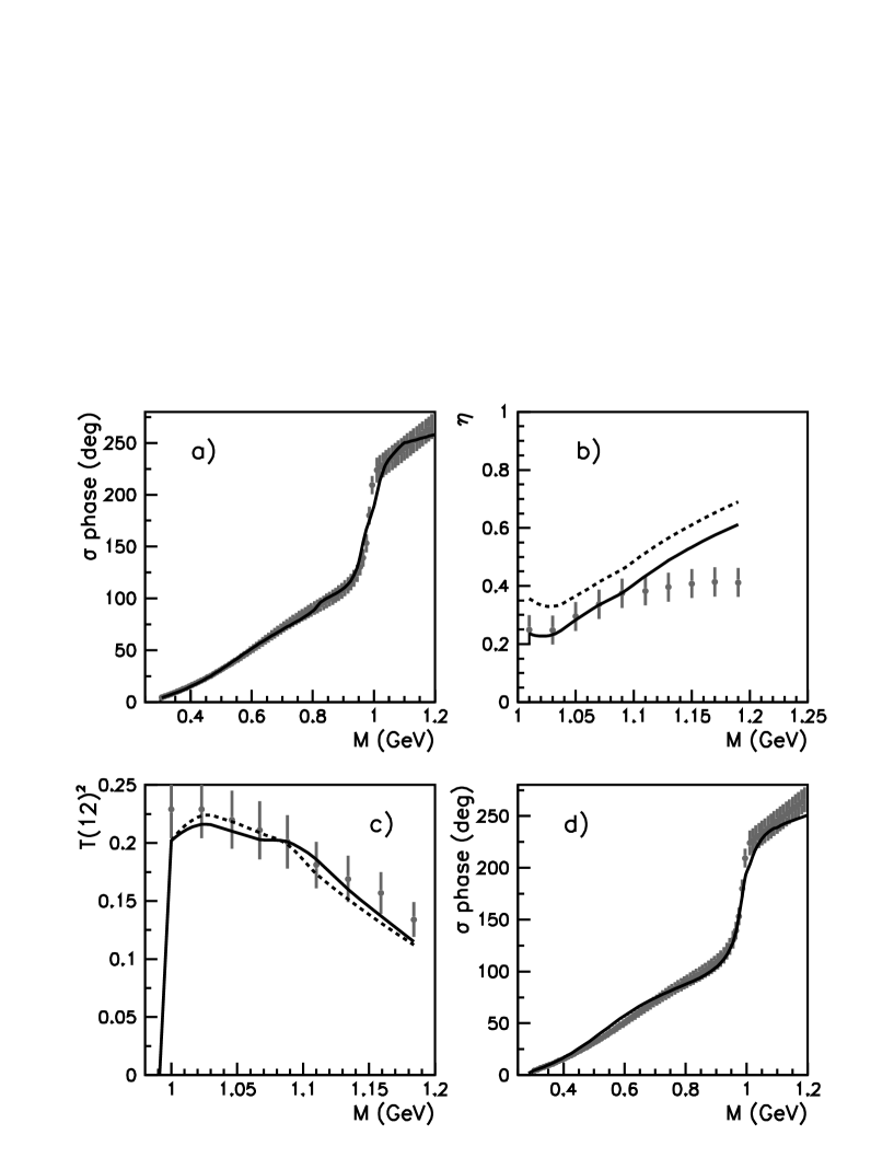
Figure 3: Fits to (a) the $\pi\pi$ phase shift with $r_{0}$, $\lambda$ and $\theta_{S}$ fitted to these data alone; (b) the elasticity parameter $\eta$ for $\pi\pi$ elastic scattering; (c) the magnitudes squared of the $T$-matrix for $\pi\pi\to KK$; and (d) as (a) with $r_{0}$, $\lambda$ and $\Theta_{S}$ fitted to all data simultaneously.

In (a), we show the recent $\pi\pi$ phases of Kaminski, Peláez and Yndurain [36] above 1 GeV. Figure 3(a) and full lines on (b) and (c) show fits to individual sets of data, varying $\lambda$, $r_{0}$ and $\theta_{S}$. This achieves a good fit to all sets of data. Figure 3(d) and the dashed lines on Figs. 3(b) and (c) show the best fit when all three sets of data are fitted simultaneously. The pole position of $f_{0}(980)$ is then at $1007-i38$ MeV, compared with the experimental value $(998\pm 4)-i(18\pm 4)$ from BES parameters.

The optimum value of $\Theta_{S}$ is $\sim\!4^{\circ}$, quite a bit smaller than frequently quoted values (see e.g. Ref. [37]). However, fitting $f_{0}(980)$ alone gives rise to a much larger $\Theta_{S}$, in excess of $30^{\circ}$. So there is a sizable, $s$-dependent dynamical contribution to the scalar mixing angle, which is largest in the vicinity of the $f_{0}(980)$, that is, near the $KK$ threshold. This is a physically appealing result of our fits in this sector.

A further detail concerns the pseudoscalar mixing angle $\Theta_{PS}$. The experimental value from Crystal Barrel is $(-17.3\pm 1.8)^{\circ}$ [38]; that is the value used here (also see Ref. [24]). However, the fit to the line-shape of $a_{0}(980)\to\eta\pi$ is sensitive to $\Theta_{PS}$. For those data, the optimum value is $\Theta_{PS}=-(7\pm 3)^{\circ}$. This value is used for Fig. 2(b). With $\Theta_{PS}=-17.3^{\circ}$, the fit is 15% too high on both sides of the peak, as shown by the dotted curve. These discrepancies might be associated with the extensive $KK$ cloud around $a_{0}(980)$ or with the $qq\bar{q}\bar{q}$ correlations proposed by Jaffe. Alternatively, small yet non-negligible contributions from higher, closed thresholds may improve the predicted $\Theta_{PS}$, as indicated by preliminary fits.

Despite the blemishes described above, the essential results are as follows. The model of Fig. 1 is capable of generating all of $\sigma$, $\kappa$, $a_{0}(980)$ and $f_{0}(980)$ dynamically via the intermediate $q\bar{q}$ loop. This is a non-perturbative effect. The overall coupling constant required for the four resonances varies by only $\pm 9\%$ and the radius parameter $r_{0}$ by $\pm 10\%$. Moreover, all scalar poles survive, with reasonable values, over the complete range of fitted parameters, so the model is very robust. The widths of these dynamical resonances decrease as the coupling constant increases. This is an essential difference from regular $q\bar{q}$ states, where, for not too large coupling, widths are roughly proportional to the square of the coupling. Nevertheless, the formation of these four resonances cannot been dissociated from the presence of a bare $q\bar{q}$ spectrum, which is crucial for the generation of dynamical resonances with moderate widths. In particular, for each ground-state bare scalar $q\bar{q}$ state, a pair of resonances is produced by coupling to the meson-meson continuum, namely one light, non-standard scalar meson, and one regular scalar in the energy region 1.3–1.5 GeV. This phenomenon was first observed two decades ago (see 2nd paper of Ref. [11]), and later confirmed, to some extent, by Törnqvist [33].

References

- [1] E. M. Aitala et al. [E791 Collaboration], Phys. Rev. Lett. 86 (2001) 765 [arXiv:hep-ex/0007027].
- [2] M. Ablikim et al. [BES Collaboration], Phys. Lett. B 598 (2004) 149 [arXiv:hep-ex/0406038].
- [3] E. M. Aitala et al. [E791 Collaboration], Phys. Rev. Lett. 89 (2002) 121801 [arXiv:hep-ex/0204018].
- [4] E. M. Aitala et al. [E791 Collaboration], Phys. Rev. D 73 (2006) 032004 [arXiv:hep-ex/0507099].
- [5] D. V. Bugg, Eur. Phys. J. A 25 (2005) 107 [Erratum-ibid. A 26 (2005) 151] [arXiv:hep-ex/0510026].
- [6] M. Ablikim et al. [BES Collaboration], Phys. Lett. B 633 (2006) 681 [arXiv:hep-ex/0506055].
- [7] D. V. Bugg, Phys. Lett. B 632 (2006) 471 [arXiv:hep-ex/0510019].
- [8] M. Ablikim et al. [BES Collaboration], Phys. Lett. B 607 (2005) 243 [arXiv:hep-ex/0411001].
- [9] R. L. Jaffe, Phys. Rev. D 15 (1977) 267.
- [10] M. D. Scadron, Phys. Rev. D 26 (1982) 239.
- [11] E. van Beveren, G. Rupp, T. A. Rijken and C. Dullemond, Phys. Rev. D 27, 1527 (1983); E. van Beveren, T. A. Rijken, K. Metzger, C. Dullemond, G. Rupp and J. E. Ribeiro, Z. Phys. C 30 (1986) 615; E. van Beveren and G. Rupp, Phys. Rev. Lett. 93 (2004) 202001 [arXiv:hep-ph/0407281].
- [12] E. van Beveren and G. Rupp, Eur. Phys. J. C 22 (2001) 493 [arXiv:hep-ex/0106077]; E. van Beveren and G. Rupp, Int. J. Theor. Phys. Group Theor. Nonlin. Opt. 11 (2006) 179 [arXiv:hep-ph/0304105]; E. van Beveren and G. Rupp, Phys. Rev. Lett. 91 (2003) 012003 [arXiv:hep-ph/0305035]; E. van Beveren, F. Kleefeld and G. Rupp, AIP Conf. Proc. 814 (2006) 143 [arXiv:hep-ph/0510120].
- [13] E. van Beveren and G. Rupp, Mod. Phys. Lett. A 19 (2004) 1949 [arXiv:hep-ph/0406242]; E. van Beveren, J. E. G. Costa, F. Kleefeld and G. Rupp, Phys. Rev. D 74 (2006) 037501 [arXiv:hep-ph/0509351].
- [14] V. V. Anisovich, A. A. Kondashov, Y. D. Prokoshkin, S. A. Sadovsky and A. V. Sarantsev, Phys. Atom. Nucl. 63 (2000) 1410 [Yad. Fiz. 63 (2000) 1410] [arXiv:hep-ph/9711319].
- [15] G. Rupp, F. Kleefeld and E. van Beveren, AIP Conf. Proc. 756 (2005) 360 [arXiv:hep-ph/0412078]; F. Kleefeld, AIP Conf. Proc. 717 (2004) 332 [arXiv:hep-ph/0310320].
- [16] D. V. Bugg, Phys. Lett. B 572 (2003) 1 [Erratum-ibid. B 595 (2004) 556].
- [17] B. Hyams et al., Nucl. Phys. B 64 (1973) 134 [AIP Conf. Proc. 13 (1973) 206].
- [18] S. Pislak et al. [BNL-E865 Collaboration], Phys. Rev. Lett. 87 (2001) 221801 [arXiv:hep-ex/0106071].
- [19] G. Colangelo, J. Gasser and H. Leutwyler, Nucl. Phys. B 603 (2001) 125 [arXiv:hep-ph/0103088].
- [20] D. Aston et al., Nucl. Phys. B 296 (1988) 493.
- [21] D. V. Bugg, Eur. Phys. J. C 47 (2006) 45 [arXiv:hep-ex/0603023].
- [22] A. Aloisio et al. [KLOE Collaboration], Phys. Lett. B 536 (2002) 209 [arXiv:hep-ex/0204012].
- [23] D. V. Bugg, V. V. Anisovich, A. Sarantsev and B. S. Zou, Phys. Rev. D 50 (1994) 4412.
- [24] F. Kleefeld, Acta Physica Slovaca 56 (2006) 373 [arXiv:nucl-th/0510017].
- [25] A. Dobado and J. R. Peláez, Phys. Rev. D 47 (1993) 4883 [arXiv:hep-ph/9301276].
- [26] J. A. Oller and E. Oset, Nucl. Phys. A 620 (1997) 438 [Erratum-ibid. A 652 (1999) 407] [arXiv:hep-ph/9702314].
- [27] J. A. Oller, E. Oset and J. R. Peláez, Phys. Rev. D 59 (1999) 074001 [Erratum-ibid. D 60 (1999) 099906] [arXiv:hep-ph/9804209].
- [28] J. A. Oller and E. Oset, Phys. Rev. D 60 (1999) 074023 [arXiv:hep-ph/9809337].
- [29] M. Jamin, J. A. Oller and A. Pich, Nucl. Phys. B 587 (2000) 331 [arXiv:hep-ph/0006045].
- [30] A. Gomez Nicola and J. R. Peláez, Phys. Rev. D 65 (2002) 054009 [arXiv:hep-ph/0109056].
- [31] F. Kleefeld, PoS HEP2005 (2006) 108 [arXiv:hep-ph/0511096].
-
[32]
G. Janssen, B. C. Pearce, K. Holinde and J. Speth,
Phys. Rev. D 52 (1995) 2690
[arXiv:nucl-th/9411021].
Also see V. Baru, J. Haidenbauer, C. Hanhart, Y. Kalashnikova and A. Kudryavtsev, Phys. Lett. B 586 (2004) 53 [arXiv:hep-ph/0308129]. - [33] N. A. Törnqvist, Z. Phys. C 68, 647 (1995) [arXiv:hep-ph/9504372]; N. A. Törnqvist and M. Roos, Phys. Rev. Lett. 76, 1575 (1996) [arXiv:hep-ph/9511210].
- [34] S. Descotes-Genon and B. Moussallam, arXiv:hep-ph/0607133.
- [35] S. Eidelman et al. [Particle Data Group], Phys. Lett. B 592 (2004) 1.
- [36] R. Kaminski, J. R. Peláez and F. J. Yndurain, arXiv:hep-ph/0603170.
- [37] R. Delbourgo and M. D. Scadron, Int. J. Mod. Phys. A 13 (1998) 657 [arXiv:hep-ph/9807504].
- [38] C. Amsler et al. [Crystal Barrel Collaboration], Phys. Lett. B 294 (1992) 451.