String deformations induced by retardation effects

Abstract

The rotating string model is an effective model of mesons, in which the quark and the antiquark are linked by a straight string. We previously developed a new framework to include the retardation effects in the rotating string model, but the string was still kept straight. We now go a step further and show that the retardation effects cause a small deviation of the string from the straight line. We first give general arguments constraining the string shape. Then, we find analytical and numerical solutions for the string deformation induced by retardation effects. We finally discuss the influence of the curved string on the energy spectrum of the model.

I Introduction

The retardation effect between two interacting particles is a relativistic phenomenon, due to the finiteness of the interaction speed. Light mesons are typical systems in which these effects can significantly contribute to the dynamics, since the light quarks can move at a speed close to the speed of light. We developed in Ref. Buis a generalization of the rotating string model (RSM) dubi94 ; guba94 in order to take into account the retardation effects in the mesons. The RSM is an effective model derived from the QCD Lagrangian, describing a meson by a quark and an antiquark linked by a straight string. Both particles are considered as spinless because spin interactions are sufficiently small to be added in perturbation. It has been shown that the RSM was classically equivalent to the relativistic flux tube model sema04 ; buis042 . This last model, firstly presented in Refs. laco89 ; tf_2 , yields meson spectra in good agreement with the experimental data tf_Semay . Our method to treat the retardation effects relies on the hypothesis that the relative time between the quark and the antiquark must have a nonzero value. Consequently, in our approach, the evolution parameter of the system is not the common proper time of the quark, the antiquark and the string, but the time coordinate of the center of mass which plays the role of an “average” time.

We showed in Ref. Buis that, in the special case where the quark and the antiquark have the same mass, the part of the total Hamiltonian containing the retardation terms could be treated as a perturbation. This perturbation is a harmonic oscillator in the relative time variable, with an effective reduced mass and an effective restoring force both depending on eigenstates of the unperturbed Hamiltonian (which is independent of the relative time). The fundamental state of this oscillator gives the contribution of the retardation to the masses as well as the relative time part of the wave function. So, the relative time wave function is a gaussian function centered around zero. This point confirms the validity of the usual non retarded model in first approximation. It is worth mentioning that our retardation term does not destroy the Regge trajectories, the linear relation between the square mass and the spin of the light mesons. Our generalized RSM also allows to reproduce the experimental meson spectrum with a good agreement.

This previous work must be considered as a first trial to compute an estimation of the retardation effects in mesons. Some hypothesis were made in order to keep the calculations workable. In particular, the straight line ansatz was used to describe the string. Although it simplifies the calculations, it is worth noting that the use of a non vanishing relative time is not really compatible with a straight string. We already gave in Ref. Buis a crude estimation of the possible bending of the string due to retardation effects, and our result was compatible with a small deviation from the straight line. However, this point deserves a further study to confirm the validity of our approach. Moreover, these deformations are of intrinsic interest, since they can exist independently of the retardation effects.

Our paper is organized as follows. In Sec. II, we briefly recall the approach developed in Ref. Buis , the RSM with a nonzero relative time. Then, assuming that the string can be curved, we give arguments constraining its possible shape in Sec. III, and we make a rather general ansatz for the curved string in Sec. IV. Using this ansatz, we obtain analytic and numerical solutions for the string shape in Secs. V and VI. Finally, we sum up our results in Sec. VII.

II Rotating string model with a nonzero relative time

The RSM with a nonzero relative time has been studied in detail in Ref. Buis . So, we simply recall here the main points of this work. Starting from the QCD Lagrangian and neglecting the spin contribution of the quark and the antiquark, the Lagrange function of a meson reads dubi94 ($\eta={\rm diag}(+---)$ and $\hbar=c=1$)

$${\cal L}=-m_{1}\sqrt{\dot{\bm{x}}^{2}_{1}}-m_{2}\sqrt{\dot{\bm{x}}^{2}_{2}}-a\int^{1}_{0}d\theta\sqrt{(\dot{\bm{w}}\bm{w}^{\prime})^{2}-\dot{\bm{w}}^{2}{\bm{w}^{\prime}}^{2}}.$$ (1)

The first two terms are the kinetic energy operators of the quark and the antiquark, whose current masses are $m_{1}$ and $m_{2}$. These two particles are attached by a string with a tension $a$. $\bm{x}_{i}$ is the coordinate of the quark $i$ and $\bm{w}$ is the coordinate of the string. $\bm{w}$ depends on two variables defined on the string world sheet: One is spacelike, $\theta$, and the other timelike, $\tau$. Derivatives are denoted $\bm{w}^{\prime}=\partial_{\theta}\bm{w}$ and $\dot{\bm{w}}=\partial_{\tau}\bm{w}$. In this picture, $\tau$ is the timelike evolution parameter for the string and the quarks. Let us mention that bold quantities will always denote four-vectors.

Introducing auxiliary fields to get rid of the square roots in the Lagrangian (1) and making the straight line ansatz to describe the string, an effective Lagrangian can be derived guba94

$${\cal L} = -\frac{1}{2}\left[\frac{m^{2}_{1}}{\mu_{1}}+\frac{m^{2}_{2}}{\mu_{2}}+a_{1}\dot{\bm{R}}^{2}+2a_{2}\dot{\bm{R}}\dot{\bm{r}}-2(c_{1}+\dot{\zeta}a_{1})\dot{\bm{R}}\bm{r}\right.$$ (2)

$$\left.-2(c_{2}+\dot{\zeta}a_{2})\dot{\bm{r}}\bm{r}+a_{3}\dot{\bm{r}}^{2}+(a_{4}+2\dot{\zeta}c_{1}+\dot{\zeta}^{2}a_{1})\bm{r}^{2}\right],$$

where the coefficients $a_{1}$, $a_{2}$, …, are functions of the auxiliary fields. Their exact expressions can be found in Ref. Buis . The parameter $\zeta$ defines the position $\bm{R}$ of the center of mass

$$\bm{R}=\zeta\bm{x}_{1}+(1-\zeta)\bm{x}_{2}\equiv(\bar{t},\vec{R}\,),$$ (3)

and $\bm{r}$ is the relative coordinate

$$\bm{r}=\bm{x}_{1}-\bm{x}_{2}\equiv(\sigma,\vec{r}\,).$$ (4)

It is worth mentioning that the auxiliary field $\mu_{i}$ can be interpreted as the constituent mass of the quark whose current mass is $m_{i}$. Moreover, the parameter $\zeta$ appears to be a function of the auxiliary fields. It reduces to the expected value $\zeta=1/2$ when the quark and the antiquark have the same mass sema04 ; buis042 . The straight line ansatz for the string implies that the string coordinates are given by

$$\bm{w}=\bm{R}+(\theta-\zeta)\bm{r}.$$ (5)

Such an ansatz is suggested by lattice QCD calculations, which show that the chromoelectric field between the quark and the antiquark appears to be roughly constant on a straight line joining the two particles Koma .

The usual approach is to work with the equal time ansatz, i. e.

$$x^{0}_{1}=x^{0}_{2}=w^{0}=\tau=\bar{t}.$$ (6)

Then, we have $\bm{r}=(0,\vec{r}\,)$, $\bm{R}=(t,\vec{R}\ )$, $\dot{\bm{r}}=(0,\dot{\vec{r}}\,)$, and $\dot{\bm{R}}=(1,\dot{\vec{R}})$. This procedure considerably simplifies the equations, but neglects the relativistic retardation effects due to a possible nonzero value of the relative time $\sigma$. That is why we made in Ref. Buis a less restrictive hypothesis: We identified the temporal coordinate of the center of mass with the evolution parameter, $\bar{t}=\tau$, and we allowed a non vanishing relative time $\sigma$. We have then

$$\dot{\bm{r}}=(\dot{\sigma},\dot{\vec{r}}\,),\ \dot{\bm{R}}=(1,\dot{\vec{R}}\,).$$ (7)

It is then possible to derive from the Lagrangian (2) a set of three equations for the RSM with a nonzero relative time

$$0 = \mu_{1}y_{1}-\mu_{2}y_{2}-\frac{ar}{y_{t}}\left(\sqrt{1-y^{2}_{1}}-\sqrt{1-y^{2}_{2}}\right),$$ (8a)

$$\frac{L}{r} = \frac{1}{y_{t}}(\mu_{1}y^{2}_{1}+\mu_{2}y^{2}_{2})+\frac{ar}{y_{t}^{2}}(F(y_{1})+F(y_{2})),$$ (8b)

$$H = \frac{1}{2}\left[\frac{p^{2}_{r}+m^{2}_{1}}{\mu_{1}}+\frac{p^{2}_{r}+m^{2}_{2}}{\mu_{2}}+\mu_{1}(1+y^{2}_{1})+\mu_{2}(1+y^{2}_{2})\right]$$ (8c)

$$+\frac{ar}{y_{t}}(\arcsin y_{1}+\arcsin y_{2})+\Delta H,$$

with

$$F(y_{i})=\frac{1}{2}\left[\arcsin y_{i}-y_{i}\sqrt{1-y^{2}_{i}}\right]\quad\text{and}\quad y_{t}=y_{1}+y_{2}.$$ (9)

$p_{r}$ is the radial momentum and $y_{i}$ is the transverse velocity of the quark $i$. The first relation gives the cancellation of the total momentum in the center of mass frame, while the two last ones define respectively the angular momentum and the Hamiltonian of the system. Equations (8a) and (8b) define the two variables $y_{1}$ and $y_{2}$. A further elimination of the auxiliary fields $\mu_{1}$ and $\mu_{2}$ yields the relativistic flux tube model buis042 .

Equations (8) are identical to those of the usual RSM (see for example Ref. buis042 ), but a perturbation of the Hamiltonian, denoted $\Delta H$, is now present. It contains the contribution of the retardation effects and is given by Buis

$$\Delta H=-\frac{\Sigma^{2}}{2a_{3}}+\frac{c_{2}}{a_{3}}\Sigma\sigma-(c_{1}+\dot{\zeta}a_{1})\sigma-\frac{c_{2}^{2}}{2a_{3}}\sigma^{2}+\frac{1}{2}(a_{4}+2\dot{\zeta}c_{1}+\dot{\zeta}^{2}a_{1})\sigma^{2},$$ (10)

where $\Sigma$ is the canonical momentum associated with the relative time $\sigma$.

Let us now consider the quantized version of our model: $L\rightarrow\sqrt{\ell(\ell+1)}$, $\left[r,\,p_{r}\right]=i$, $\left[\sigma,\,\Sigma\right]=-i$. The Hamiltonian (8c) has then the following structure

$$H(\sigma,r)=H_{0}(r)+\Delta{H}(\sigma,r).$$ (11)

The relative time only appears in the perturbation, and $H_{0}$ depends only on the radius $r$. So, we can assume that the total wave function reads

$$\left|\psi(\bm{r})\right\rangle=\left|A(\sigma)\right\rangle\otimes\left|R(r)\right\rangle\otimes\left|Y_{\ell\,m}(\theta,\phi)\right\rangle,$$ (12)

where $\left|R(r)\right\rangle$ is a solution of the eigenequation

$$H_{0}(r)\left|R(r)\right\rangle=M_{0}\left|R(r)\right\rangle.$$ (13)

Such a problem can be solved for instance by the Lagrange mesh technique buis041 . As it is shown in Ref. Buis , the total mass is written

$$M = M_{0}+\left\langle A(\sigma)\right|\otimes\left\langle R(r)\right|\Delta H(r,\sigma)\left|R(r)\right\rangle\otimes\left|A(\sigma)\right\rangle$$ (14)

$$= M_{0}+\Delta M.$$

The contribution $\Delta M$ is then given by the fundamental state of the eigenequation

$$\Delta{\cal H}(\sigma)\left|A(\sigma)\right\rangle=\Delta M\left|A(\sigma)\right\rangle,$$ (15)

where

$$\Delta{\cal H}(\sigma)=\left\langle R(r)\right|\Delta H(r,\sigma)\left|R(r)\right\rangle.$$ (16)

In the case $m_{1}=m_{2}$, the eigenequation (15) can be solved, since $\Delta{\cal H}(\sigma)$ is simply a harmonic oscillator in the relative time $\sigma$

$$\Delta{\cal H}(\sigma)=-\frac{1}{2\langle a_{3}\rangle}\left[\Sigma^{2}+\langle c_{2}^{2}-a_{4}a_{3}\rangle\sigma^{2}\right].$$ (17)

A more detailed study of the retardation term $\Delta M$ and of its effect on the meson spectrum can be found in Ref. Buis . Let us only observe two points from Eqs. (15) and (17). Firstly, the retardation contribution $\Delta M$ is negative,

$$\Delta M=-\frac{1}{2}\sqrt{\langle c_{2}^{2}-a_{4}a_{3}\rangle/\langle a_{3}\rangle^{2}},$$ (18)

and it thus decreases the meson mass. Secondly, the temporal part of the wave function reads

$$A(\sigma)=\left(\frac{\beta}{\pi}\right)^{1/4}\exp\left(-\frac{\beta}{2}\sigma^{2}\right),$$ (19)

with

$$\beta=\sqrt{\langle c_{2}^{2}-a_{4}a_{3}\rangle}.$$ (20)

It is a gaussian function centered around $\sigma=0$. This provides an interpretation of the equal time ansatz (6) as the most probable configuration of the system.

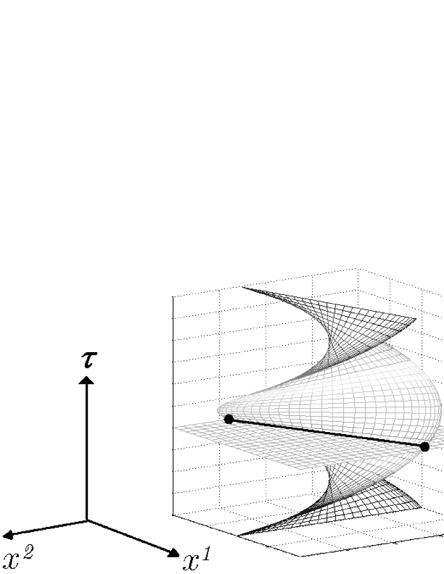
Figure 1: Left: Intersection between a helicoidal string world sheet and a plane $\tau=\tau_{0}$ ($x^{0}_{q}(\tau_{0})=x^{0}_{\bar{q}}(\tau_{0})$), the intersection is a straight line. Right: Same situation, but now $x^{0}_{q}(\tau_{0})\neq x^{0}_{\bar{q}}(\tau_{0})$, and the intersection is curved.

It is worth noting that the use of a non vanishing relative time is not really compatible with the straight line ansatz. This can be seen by the following simple considerations: Let us assume that the world sheet of the system in the center of mass frame is a helicoid area in the case of exactly circular quark orbits. The shape of the string is then a straight line for a slice at constant time and a curve for a slice not at constant time (see Fig. 1). We already gave in Ref. Buis a crude estimation of the possible bending of the string due to retardation effects, and our result was compatible with a small deviation from the straight line. The purpose of this paper is to study more carefully the string deformations caused by the nonzero relative time in order to confirm the validity of our approach.

III Constraints on the string shape

As the coordinates $\bm{x}_{i}$ are independent of the parameter $\theta$, the Lagrangian (1) can be rewritten as

$${\cal L}=\int^{1}_{0}d\theta{\cal\tilde{L}},$$ (21)

with

$${\cal\tilde{L}}=-m_{1}\sqrt{\dot{\bm{x}}^{2}_{1}}-m_{2}\sqrt{\dot{\bm{x}}^{2}_{2}}-a\sqrt{(\dot{\bm{w}}\bm{w}^{\prime})^{2}-\dot{\bm{w}}^{2}{\bm{w}^{\prime}}^{2}}.$$ (22)

Several steps are required to obtain a Hamiltonian from the Lagrangian (22). Firstly, one has to find a particular solution, denoted $\bm{w}^{*}$, for the string shape. This is in fact the solution of the equations of motion (EOM) of the Nambu-Goto Lagrangian

$${\cal\tilde{L}}_{NG}=-a\sqrt{(\dot{\bm{w}}\bm{w}^{\prime})^{2}-\dot{\bm{w}}^{2}{\bm{w}^{\prime}}^{2}},$$ (23)

with the boundary conditions

$$\bm{w}(1,\tau)=\bm{x}_{1}(\tau),\ \ \bm{w}(0,\tau)=\bm{x}_{2}(\tau).$$ (24)

Secondly, once $\bm{w}^{*}$ is known, it has to be injected in the total Lagrangian (22). Thirdly, one has to compute the momenta defined by

$$p_{i\mu}=\frac{\partial{\cal\tilde{L}}}{\partial\dot{x}^{\mu}_{i}}.$$ (25)

In this picture, we assume that $\bm{w}^{*}(\theta,\tau)$ is in fact of the form $\bm{w}^{*}(\theta,\bm{x}_{i}(\tau))$, because of the boundary conditions (24). Finally, with the momenta (25), the quantity

$${\cal\tilde{H}}=\sum^{2}_{i=1}\bm{p}_{i}\dot{\bm{x}}_{i}-{\cal\tilde{L}}$$ (26)

is readily computed, and the total Hamiltonian is thus given by

$${\cal H}=\int^{1}_{0}d\theta{\cal\tilde{H}}.$$ (27)

In the usual RSM, one uses the straight line ansatz (5) together with the equal time ansatz (6). This provides indeed a correct solution $\bm{w}^{*}$ of the EOM (str, , p. 122). The question we want to answer in this section is: Is it possible to find a more general form for the string shape?

Let us suppose that we have such a solution, $\bm{w}^{*}$, which thus respects the conditions (24). As we already remarked, $\bm{w}^{*}$ depends on the coordinates $\dot{\bm{x}}_{i}(\tau)$. So, the momenta (25) read

$$p_{i\mu}=-m_{i}\frac{\dot{x}_{i\mu}}{\sqrt{\dot{\bm{x}}^{2}_{i}}}-a\frac{N_{\rho}}{\sqrt{\bm{N}\dot{\bm{w}}}}\frac{\partial\dot{w}^{\rho}}{\partial\dot{x}^{\mu}_{i}},$$ (28)

with

$$\bm{N}=(\dot{\bm{w}}\bm{w}^{\prime})\bm{w}^{\prime}-\bm{w}^{\prime 2}\dot{\bm{w}}.$$ (29)

For the sake of simplicity, we have dropped the ^∗ on $\bm{w}$. The Hamiltonian (26), computed with the momenta (28), is expected to vanish since we work in a manifestly covariant formalism. Here, we see that

$${\cal H}=a\left[\sqrt{\bm{N}\dot{\bm{w}}}-\sum^{2}_{i=1}\frac{N_{\rho}}{\sqrt{\bm{N}\dot{\bm{w}}}}\frac{\partial\dot{w}^{\rho}}{\partial\dot{x}^{\mu}_{i}}\dot{x}^{\mu}_{i}\right].$$ (30)

If we want ${\cal H}=0$, we must satisfy the condition

$$\dot{w}^{\rho}=\sum^{2}_{i=1}\frac{\partial\dot{w}^{\rho}}{\partial\dot{x}^{\mu}_{i}}\dot{x}^{\mu}_{i}.$$ (31)

The solution for the constraint (31) is

$$\dot{w}^{\rho}(\theta,\tau)=\sum^{2}_{i=1}A^{\rho}_{i\nu}(\theta,\tau)\dot{x}^{\nu}_{i}(\tau),$$ (32)

where the $A^{\rho}_{i\nu}(\theta,\tau)$ are unspecified functions. A simple integration gives

$$w^{\rho}(\theta,\tau)=\sum^{2}_{i=1}A^{\rho}_{i\nu}(\theta,\tau)x^{\nu}_{i}(\tau)-\sum^{2}_{i=1}\int^{\tau}_{0}d\tilde{\tau}\dot{A}^{\rho}_{i\nu}(\theta,\tilde{\tau})x^{\nu}_{i}(\tilde{\tau})+f^{\rho}(\theta).$$ (33)

Expressing Eq. (33) in the center of mass and relative coordinates, given by relations (3) and (4), we obtain

$$w^{\rho} = (A^{\rho}_{1\nu}+A^{\rho}_{2\nu})R^{\nu}+\left[(1-\zeta)A^{\rho}_{1\nu}-\zeta A^{\rho}_{2\nu}\right]r^{\nu}$$

$$-\int d\tilde{\tau}\left\{(\dot{A}^{\rho}_{1\nu}+\dot{A}^{\rho}_{2\nu})R^{\nu}+\left[(1-\zeta)\dot{A}^{\rho}_{1\nu}-\zeta\dot{A}^{\rho}_{2\nu}\right]r^{\nu}\right\}+g^{\rho},$$

if we assume that $\dot{\zeta}=0$. We did not write explicitly the dependences in $(\theta,\tau)$ to clarify the notations.

Formula (III) can be simplified by taking the limit $\bm{r}\rightarrow 0$. In this case, we want indeed to obtain $\bm{w}=\bm{R}$. This clearly implies that

$$A^{\rho}_{1\nu}+A^{\rho}_{2\nu}=\delta^{\rho}_{\nu},\ \ g^{\rho}=0,$$ (35)

and the whole expression (III) can thus be rewritten by using a single set of functions $A^{\rho}_{\nu}\equiv A^{\rho}_{1\nu}$

$$w^{\rho}=R^{\rho}+(A^{\rho}_{\nu}-\zeta\delta^{\rho}_{\nu})r^{\nu}-\int d\tau\dot{A}^{\rho}_{\nu}r^{\nu}.$$ (36)

The solution (36) is the general string shape we search for. Solving the corresponding EOM would allow us to determine the functions $A^{\rho}_{\nu}$. However, this problem is very complex, and we need to make some simplifications to go further. We want to find a solution which corresponds to a string configuration which does not change in time. So we consider the functions $A^{\rho}_{\nu}$ to be independent of $\tau$. We also make the following hypothesis

$$A^{\rho}_{\nu}=A^{\rho}\delta^{\rho}_{\nu},$$ (37)

without summation on $\rho$. This implies that we want $w^{\mu}$ depending only on the coordinates $R^{\mu}$ and $r^{\mu}$. With our assumptions, the string has finally the following form

$$w^{\mu}(\theta,\tau)=R^{\mu}(\tau)+\left[A^{\mu}(\theta)-\zeta\right]r^{\mu}(\tau),$$ (38)

without summation on $\mu$. The remaining unknown quantities are the functions $A^{\mu}(\theta)$. Let us note that the straight string ansatz is only a particular case of formula (38), where $A^{\mu}(\theta)=\theta$.

IV The curved string ansatz

In order to further simplify the problem, we will here consider mesons in which the quark and the antiquark have the same mass. In this case, $\zeta=1/2$, and only the part of the string linking the center of mass and one quark has to be known. The second part can be computed from the first one by using symmetry arguments, as it will be discussed in Sec. VI. Formally, we thus only have to find a solution for $\bm{w}(\rho,\tau)$ with $\rho\in\left[0,1\right]$, such that

$$\bm{w}(0,\tau)=\bm{R},\ \ \bm{w}(1,\tau)=\bm{r}_{q}(\tau),$$ (39)

$\bm{r}_{q}(\tau)$ being the position of the quark, for instance. As we work in the center of mass frame, we can set $\bm{R}=(\bar{t},\vec{0}\,)$. We can then rewrite Eq. (38) on the following form

$$w^{0}(\rho,\tau) = \bar{t}(\tau)+A^{0}(\rho)r^{0}_{q}(\tau),$$ (40a)

$$w^{i}(\rho,\tau) = A^{i}(\rho)r^{i}_{q}(\tau).$$ (40b)

The meson evolves in a plane. We can thus set $A^{3}$ equal to zero and use the complex coordinates $(w^{0},w,w^{*})$ defined by Olss

$$w=\frac{1}{\sqrt{2}}(w^{1}+iw^{2}).$$ (41)

The Nambu-Goto Lagrangian is invariant for the reparameterization of the world sheet (str, , p. 93), that is to say the transformations

$$\tau^{\prime}=\tau^{\prime}(\rho,\tau),\ \ \rho^{\prime}=\rho^{\prime}(\rho,\tau).$$ (42)

It allows us to fix for simplicity

$$\bar{t}(\tau)=\tau,\quad{\rm and}\quad A^{1}(\rho)=\rho.$$ (43)

In the following, the relations (43) will always be assumed. Let us note that $\bar{t}(\tau)=\tau$ was a hypothesis of the model in Ref. Buis .

It can be shown that, when $r^{0}_{q}(\tau)=0$,

$$w^{0}(\rho,\tau) = \tau,$$ (44a)

$$w(\rho,\tau) = \frac{r_{q}(\tau)}{\sqrt{2}}\,\rho\,\exp\left[i\omega\tau\right],$$ (44b)

is a solution of the EOM of the Nambu-Goto, or equivalently, of the Polyakov Lagrangian (see for example Ref. Olss ). In our coordinates, these EOM read

$$\partial_{a}\left[\sqrt{-h}\,h^{ab}\partial_{b}w^{\mu}\right]=0,$$ (45a)

with $$h^{ab} h_{ab}$$ the inverse matrix of , given by

$$h_{ab} = \partial_{a}w^{\mu}\partial_{b}w_{\mu},$$ (45b)

$$= -\partial_{a}w^{0}\partial_{b}w^{0}+2{\rm Re}\left(\partial_{a}w^{*}\partial_{b}w\right).$$

The indices $(a,b)$ label the parameters $(\tau,\rho)$, and $h_{ab}$ is the induced metric on the string world sheet.

Solution (44) describes a straight string with a constant angular speed, and it corresponds to the following choices in Eqs. (40): $r^{0}_{q}(\tau)=0$, $A^{2}(\rho)=\rho$, $r^{1}_{q}(\tau)=r_{q}(\tau)\cos\omega\tau$, and $r^{2}_{q}(\tau)=r_{q}(\tau)\sin\omega t$.

In our previous work on the retardation effects, we used the following ansatz Buis

$$w^{0}(\rho,\tau) = \tau+\rho\,\sigma_{q}(\tau),$$ (46a)

$$w(\rho,\tau) = \frac{r_{q}(\tau)}{\sqrt{2}}\,\rho\exp(i\omega\tau),$$ (46b)

that is to say $r^{0}_{q}(\tau)=\sigma_{q}(\tau)$, $A^{0}(\rho)=A^{2}(\rho)=\rho$, $r^{1}_{q}(\tau)=r_{q}(\tau)\cos\omega\tau$, and $r^{2}_{q}(\tau)=r_{q}(\tau)\sin\omega t$. However, the string defined by Eqs. (46) is not a solution of the EOM. Indeed, as $\sigma_{q}(\tau)$ is assumed to be small (we showed that the retardation can be treated as a perturbation), we can write the EOM at the first order in $\sigma_{q}$. After some calculations, one can check from relations (45) that $\sigma_{q}$ must satisfy the following equation

$$r^{2}_{q}\rho^{2}\ddot{\sigma}_{q}-2r_{q}\dot{r}_{q}\rho^{2}\dot{\sigma}_{q}+\left[\left(r^{2}_{q}\omega^{2}-r_{q}\ddot{r}_{q}+2\dot{r}^{2}_{q}\right)\rho^{2}-2\right]\sigma_{q}=0.$$ (47)

As $\sigma_{q}$ is only a function of $\tau$, Eq. (47) must be satisfied for every value of $\rho$. In particular, when $\rho=0$, we observe that $\sigma_{q}=0$ is the only possible solution. This confirms that a straight string is not compatible with a nonzero relative time.

Finally, it appears quite natural that the string could be curved because of the addition of two effects: The rotation of the meson and the finiteness of the gluon speed. A curved string can be described by the ansatz

$$w^{0}(\rho,\tau) = \tau+\rho\,\sigma_{q}(\tau),$$ (48a)

$$w(\rho,\tau) = \frac{r_{q}(\tau)}{\sqrt{2}}\,\left[\rho+if(\rho)\right]\exp\left[i(\omega\tau+\phi(\tau)\right],$$ (48b)

where the spatial deformation $f(\rho)$ has been introduced as a counterpart to the relative time $\sigma_{q}(\tau)$. Moreover, the eventuality of a non constant rotation speed is taken into account through the angular acceleration $\phi(\tau)$. If $\sigma_{q}=0$, our ansatz reduces to the one of Ref. Olss , where the string deformations due to angular acceleration are studied. Equations (48) clearly describe a curved string, as it can be seen by rewriting it when $\tau=0$ with $\phi(0)=0$. Then we have simply $w^{1}\propto\rho$ and $w^{2}\propto f(\rho)$.

V Analytic solution

Finding an exact expression of $f(\rho)$ which satisfies the EOM of the Nambu-Goto Lagrangian is a very complex problem, out of the scope of this paper. The use of approximations appears necessary in order to deal with workable equations. We have given in Ref. Buis some arguments to show that the deformation of the string should be small. Assuming that point, we will linearize the EOM in $f(\rho)$ and its derivatives. The angular acceleration will also be considered as small, as it is done in Ref. Olss . Following the hypothesis of this last reference, we will only keep the linear terms in $\phi$ and its derivatives. Terms like $\phi f,\,\phi\sigma_{q},\,\phi\dot{\sigma_{q}},\,\phi\dot{r}_{q},\dots$ will thus also be neglected. Moreover, we consider that $\ddot{r}_{q},\,\ddot{\sigma_{q}}\approx 0$. Consequently, our solution will only be valid in the case of small radial excitations.

After a tedious algebra, we find that the EOM (45) are satisfied by the curved string (48) if

$$\left(1-A_{1}\rho-A_{2}\rho^{2}+A_{3}\rho^{3}\right)\partial^{2}_{\rho}f(\rho)+(B_{1}-B_{2}\rho)\left(\rho\partial_{\rho}f(\rho)-f(\rho)\right)=C+D\rho-E\rho^{2},$$ (49)

with

$$A_{1} = \sigma_{q}\frac{\dot{r}_{q}}{r_{q}}-3\dot{\sigma_{q}},$$ (50a)

$$A_{2} = \omega^{2}r^{2}_{q}+\dot{r}^{2}_{q}+2\sigma_{q}\dot{\sigma_{q}}\frac{\dot{r}_{q}}{r_{q}}-3\dot{\sigma_{q}}^{2},$$ (50b)

$$A_{3} = \omega^{2}\sigma_{q}r_{q}\dot{r}_{q}+\sigma_{q}\frac{\dot{r}^{3}_{q}}{r_{q}}-\omega^{2}\dot{\sigma_{q}}r^{2}_{q}-\dot{\sigma_{q}}\dot{r}^{2}_{q}-\sigma_{q}\dot{\sigma_{q}}^{2}\frac{\dot{r}_{q}}{r_{q}}+\dot{\sigma_{q}}^{3},$$ (50c)

$$B_{1} = \omega^{2}r^{2}_{q}+3\omega^{2}\sigma_{q}^{2}+2\sigma_{q}^{2}\frac{\dot{r}^{2}_{q}}{r^{2}_{q}}-2\sigma_{q}\dot{\sigma_{q}}\frac{\dot{r}_{q}}{r_{q}},$$ (50d)

$$B_{2} = 2\omega^{2}\sigma_{q}r_{q}\dot{r}_{q}+2\sigma_{q}\frac{\dot{r}^{3}_{q}}{r_{q}}+\omega^{2}\dot{\sigma_{q}}r^{2}_{q}-3\omega^{2}\dot{\sigma_{q}}\sigma_{q}^{2}-2\dot{\sigma_{q}}\dot{r}^{2}_{q}+2\sigma_{q}^{2}\dot{\sigma_{q}}\frac{\dot{r}^{2}_{q}}{r^{2}_{q}}+2\sigma_{q}\dot{\sigma_{q}}^{2}\frac{\dot{r}_{q}}{r_{q}},$$ (50e)

$$C = 2\sigma_{q}\omega,$$ (50f)

$$D = 2\omega\sigma_{q}\dot{\sigma_{q}}-2\omega\sigma_{q}^{2}\frac{\dot{r}_{q}}{r_{q}}+r^{2}_{q}\ddot{\phi},$$ (50g)

$$E = -\omega^{3}\sigma_{q}r^{2}_{q}+\omega^{3}\sigma_{q}^{3}-2\omega\sigma_{q}\dot{r}^{2}_{q}+2\omega\sigma_{q}^{3}\frac{\dot{r}^{2}_{q}}{r_{q}}+2\omega\dot{\sigma_{q}}r_{q}\dot{r_{q}}-2\omega\sigma_{q}^{2}\dot{\sigma_{q}}\frac{\dot{r}_{q}}{r_{q}},$$ (50h)

and the boundary conditions

$$f(0)=f(1)=0.$$ (51)

Conditions (51) are in fact equivalent to the initial boundary conditions (39).

Before performing a numerical resolution of the differential equation (49), we can find an approximate analytic solution by developing $f(\rho)$ in powers of $\rho$,

$$f(\rho)=\sum^{\infty}_{n=0}a_{n}\rho^{n}.$$ (52)

Keeping in this series only the terms which satisfy Eqs. (49) and (51) at the second order in $\rho$, one can find that

$$f(\rho)=f_{C}(\rho)+f_{D}(\rho)+f_{E}(\rho),$$ (53)

with

$$f_{C}(\rho) = -\frac{C}{2}\,\rho\,(1-\rho),$$ (54a)

$$f_{D}(\rho) = -\frac{(D+CA_{1})}{6}\ \rho\,(1-\rho^{2}),$$ (54b)

$$f_{E}(\rho) = \frac{1}{12}\left[E-A_{1}(D+CA_{1})-C(A_{2}-B_{1}/2)\right]\ \rho\ (1-\rho^{3}).$$ (54c)

The solution at the lowest order is $f_{C}(\rho)$. It is a parabola whose maximum is reached in $\rho=1/2$. The next functions, $f_{D}(\rho)$ and $f_{E}(\rho)$, shift slightly the maximum at a value $\rho<1/2$. A graphical representation of the solution (53) is given in the next section. It is worth mentioning that in the case of a vanishing angular momentum, $\omega=0$, the solution is trivially $f(\rho)=0$. Even when the retardation is included, the string is straight when the angular momentum is zero.

We can check that if $\sigma_{q}=0$, our solution reduces to

$$\left.f(\rho)\right|_{\sigma_{q}=0}=-\frac{r^{2}_{q}\ddot{\phi}}{6}\rho(1-\rho^{2}),$$ (55)

which is precisely the result of Ref. Olss . However, as we are only interested in the retardation effects, we will take $\ddot{\phi}=0$ in the latter.

VI Numerical solution

VI.1 Evaluation of the coefficients

The previous section gave us a qualitative idea of the string shape. But, to complete our analysis, we need an estimation of the magnitude of the deformation. To do this, we have to compute numerically the different coefficients (50), not in the classical framework we used up to now, but in a quantized model. The coefficients (50) should then be seen as operators whose average value has to be computed. What should be done rigorously is to rewrite our RSM Hamiltonian with a curved string solution of Eq. (49) and compute the eigenstates of this model to average the operators (50), in an analog way of what is done in Ref. Olss2 . But here, we only want to have a first estimation of the string deformation. That is why, as we considered that the deformation was small, it appears reasonable to compute the mean values of the coefficients (50) with the states of our particular RSM introduced in Ref. Buis . Let us remark that, if we want to be consistent with the notations for $r$ and $\sigma$ in Sec. II, we have to make the following substitutions

$$r_{q}\rightarrow r/2,\quad\sigma_{q}\rightarrow\sigma/2,$$ (56)

the angular speed $\omega$ being not modified. Our procedure will be to replace each positive definite operator $X$ appearing in the definitions (50) by $\sqrt{\left\langle X^{2}\right\rangle}$, a quantity easy to compute with our numerical method buis041 . This simple computation, neglecting symmetrization problems, will only give us a rough estimation of the different coefficients, but it is sufficient for our purpose.

We already mentioned that our numerical method, the Lagrange mesh method, ensures us to know the radial wave function $\left|R(r)\right\rangle$. The average values $\left\langle\vec{p}\,^{2}\right\rangle=\left\langle p^{2}_{r}+\ell(\ell+1)/r^{2}\right\rangle$ and $\left\langle r^{2}\right\rangle$ are easy to compute buis041 . Moreover, it is shown in Ref. buis05b that the angular speed can be approximated by

$$\omega\approx\frac{\sqrt{\ell(\ell+1)}}{\left\langle r^{2}\right\rangle\left(\left\langle\sqrt{\vec{p}\,^{2}+m^{2}}\right\rangle+a\left\langle r\right\rangle/6\right)},$$ (57)

where $\ell$ is the orbital angular momentum. The last spatial term we need is $\langle\dot{r}^{2}\rangle$, which is the radial part of $\left\langle\dot{\vec{r}}\,^{2}\right\rangle$. It can be computed, from the Lagrangian (2), that buis042

$$\left\langle p^{\,2}_{r}\right\rangle=\left\langle(a_{3}\dot{r}-c_{2}r)^{2}\right\rangle.$$ (58)

Using the fact that $\left\langle c_{2}\right\rangle\approx 0$ Buis , we have

$$\left\langle\dot{r}^{2}\right\rangle\approx\frac{1}{\left\langle a_{3}\right\rangle^{2}}\left[\left\langle p^{\,2}_{r}\right\rangle-\left\langle c^{2}_{2}\right\rangle\left\langle r^{2}\right\rangle\right].$$ (59)

We turn now our attention to the terms involving the relative time. With the temporal wave function given by Eq. (19), it is easily computed that

$$\sqrt{\left\langle\sigma^{2}\right\rangle}=\frac{1}{\sqrt{2\beta}}.$$ (60)

$\langle\dot{\sigma}^{2}\rangle$ can be computed in analogy with $\langle\dot{r}^{2}\rangle$. From the Lagrangian (2), it can be shown that Buis

$$\left\langle\Sigma^{2}\right\rangle=\left\langle\left(c_{2}\sigma-a_{3}\dot{\sigma}\right)^{2}\right\rangle.$$ (61)

Since

$$\left\langle\Sigma^{2}\right\rangle=\frac{\beta}{2},$$ (62)

we have

$$\left\langle\dot{\sigma}^{2}\right\rangle\approx\frac{\beta}{2\left\langle a_{3}\right\rangle^{2}}\left[1-\frac{\left\langle c^{2}_{2}\right\rangle}{\beta^{2}}\right].$$ (63)

We are now able to compute, at least in first approximation, the coefficients (50).

VI.2 Results

The more interesting case is the meson formed of two massless quarks. The deformation of the string is indeed expected to be maximal in this case since the relativistic effects are the most important. Of course, we will choose $\ell\neq 0$ to observe a nonzero deformation. With $m=0$ and the standard value $a=0.2$ GeV², we can compute the needed average values thanks to formulas (57) to (63). They are given in Table 1 for three different states.

Table 1: Average values of quantities involved in the coefficients (50), for different states. For simplicity, the quantities of the form $\sqrt{\langle X^{2}\rangle}$ appearing in the first column are denoted as $X$. We recall that $r_{q}=r/2$ and $\sigma_{q}=\sigma/2$.

(n+1)L	1P	1F	2P
$r_{q}$ (GeV-1)	2.526	3.376	3.411
$\sigma_{q}$ (GeV-1)	1.093	1.072	1.122
$\omega$ (GeV)	0.086	0.087	0.036
$\dot{r}_{q}$	0.459	0.303	0.592
$\dot{\sigma}_{q}$	0.342	0.257	0.252

A numerical integration of Eq. (49) to obtain the solution $f(\rho)$ with the boundary conditions (51) can be performed by using the values of Table 1. As mentioned in Sec. IV, one half of the string is simply given by the couples $\left\{\rho,f(\rho)\right\}$. Once this solution is known, we can compute every couple $\left\{\theta,\tilde{f}(\theta)\right\}$ between the quark and the antiquark. Indeed, a simple symmetry argument allows us to write

$$\left\{\theta,\tilde{f}(\theta)\right\}=\left\{\begin{array}[]{ll}\left\{(1+\rho)/2,\,f(\rho)\right\}&\theta\in\left[1/2,1\right],\\ \left\{(1-\rho)/2,\,-f(\rho)\right\}&\theta\in\left[0,1/2\right].\end{array}\right.$$ (64)

Relations (64) simply define a central symmetry with respect to the center of mass. The numerical solution of Eq. (49) is plotted in Fig. 2 for the three states considered in Table 1.

We found that the deformation is maximal for the $1F$ state, and then decreases when the quantum numbers increase. This is a consequence of our approach, since we noticed in Ref. Buis that the retardation effects are less large when the dynamical quark mass $\langle\sqrt{\vec{p}\,^{2}+m^{2}}\rangle$ increases. In every case, the deformation $f(\theta)$ is small with respect to one. This is an a posteriori validation of our choice to consider small deformations only.

Figure 2: Numerical solution of Eq. (49), giving the string shape between the quark and the antiquark for the states considered in Table 1. $f(\theta)=0$ corresponds to the straight line ansatz.

Figure 3: Comparison between the numerical solution of Eq. (49) for the $1P$ state and the analytical formula (53).

In Fig. 3, we compare the numerical solution for the $1P$ state, the lowest state in which the deformation occurs, with three analytic approximations of this solution, given by relations (53) and (54). It appears that $f_{C}$ is an upper bound of the deformation, and that $f_{C}+f_{D}$ is sufficient to correctly approximate the numerical solution.

Since the string brings an energetic contribution to the meson which is proportional to its length, it is interesting to evaluate the ratio between the lengths of both the curved and the straight strings. It is given by

$$\frac{\Delta L}{L} = \left[\int^{1}_{0}d\rho\sqrt{1+(\partial_{\rho}f)^{2}}\right]-1,$$ (65)

$$\approx \int^{1}_{0}d\rho\frac{(\partial_{\rho}f)^{2}}{2}.$$ (66)

For a small deformation, as it is the case here, we can obtain an upper bound for $\Delta L/L$ by using $f_{C}$ instead of $f$. To the second order in $C$, we find that

$$\frac{\Delta L}{L}\leq\frac{C^{2}}{24},$$ (67)

with $C=2\sigma_{q}\omega$. It is maximal in the $1F$ state. We finally obtain the upper bound

$$\frac{\Delta L}{L}\leq 2\times 10^{-3}.$$ (68)

The length of the string is only modified by some tenths of percent, because of the bending induced by retardation effects. As the typical mass scale for the mesons is the 1-2 GeV, the correction due to curved string is around 1-4 MeV, as it is observed in Ref. Olss2 . The contribution of the bending of the string to the mass spectrum seems thus very small. This is also small compared with the retardation contribution, which can be around 100 MeV for massless quarks.

VII Conclusion

We developed in this paper the idea that, if the retardation effects are included in the rotating string model, the string linking the quark and the antiquark cannot remain a straight line. We found a relation constraining its shape, and obtained a general form for the string. The straight line ansatz, which is valid in the equal time approximation, appears to be only a particular case of our general form. When the retardation is included, we showed that a bending of the string must be taken into account, and we proposed a general ansatz defining a curved string. With this ansatz, and assuming a priori that the deformation of the string is small, we derived a differential equation giving its shape. Analytical and numerical solutions of this equation can be found. Roughly, the deformed string has a parabolic shape, with a small amplitude. The amplitude of the deformation decreases when the quantum numbers increase; but it is zero for a vanishing angular momentum. We finally argued that the contribution of the bending of the string to the mass spectrum is around 1-4 MeV. The typical meson mass scale is around 1-2 GeV, and the retardation contribution computed in a previous work with a straight string is always smaller than 100 MeV. So, the effects of the curvature are very weak, although rather interesting from a theoretical point of view. However, if one is mainly interested in the computation of a mass spectrum, we can conclude from our present work that the rotating string with nonzero relative time can give satisfactory results, event with a straight string approximation. We leave the analysis of the rotating string model equations with nonzero relative time and curved string for future work.

- (1) F. Buisseret and C. Semay, Phys. Rev. D 72, 114004 (2005) [hep-ph/0505168].
- (2) A. Yu. Dubin, A. B. Kaidalov, and Yu. A. Simonov, Phys. Atom. Nucl. 56, 1745 (1993); Yad. Fiz. 56, 213 (1993) [hep-ph/9311344].
- (3) E. L. Gubankova and A. Yu. Dubin, Phys. Lett. B 334, 180 (1994) [hep-ph/9408278].
- (4) C. Semay, B. Silvestre-Brac, and I. M. Narodetskii, Phys. Rev. D 69, 014003 (2004) [hep-ph/0309256].
- (5) F. Buisseret and C. Semay, Phys. Rev. D 70, 077501 (2004) [hep-ph/0406216].
- (6) D. LaCourse and M. G. Olsson, Phys. Rev. D 39, 2751 (1989).
- (7) M. G. Olsson and S. Veseli, Phys. Rev. D 51, 3578 (1995).
- (8) C. Semay and B. Silvestre-Brac, Phys. Rev. D 52, 6553 (1995).
- (9) Y. Koma, E. M. Ilgenfritz, T. Suzuki, and H. Toki, Phys. Rev. D 64, 014015 (2001) [hep-ph/0011165].
- (10) F. Buisseret and C. Semay, Phys. Rev. E 71, 026705 (2005) [hep-ph/0409033].
- (11) B. Zwiebach, A first course in string theory, Cambridge University Press, 2004.
- (12) T. J. Allen, M. G. Olsson and S. Veseli, Phys. Rev. D 59, 094011 (1999) [hep-ph/9810363].
- (13) T. J. Allen, M. G. Olsson and S. Veseli, Phys. Rev. D 60, 074026 (1999) [hep-ph/9903222].
- (14) F. Buisseret and C. Semay, Phys. Rev. D 71, 034019 (2005) [hep-ph/0412361].