Selected topics in $e^{+}e^{-}$ - collisions

Victor L. Chernyak,

1) The leading twist pion wave function
2) ”Improved” QCD sum rules with non-local condensates
3) Pion and kaon form factors and charmonium decays:
                           theory vs experiment
4) $\gamma^{*}\gamma\pi^{o}$ - form factor
5) The new non-local axial anomaly
6) Cross sections $\gamma\gamma\rightarrow\pi^{+}\pi^{-},\,K^{+}K^{-},\,K_{S}K_{S}$

1. The leading twist pion wave function

The general formula for the leading term of the hadron form factor in QCD was first obtained in [1] and has the form :

$$\langle p_{2},\,s_{2},\,\lambda_{2}|J_{\lambda}|p_{1},\,s_{1},\,\lambda_{1}\rangle=C_{12}\Bigl{(}\frac{1}{\sqrt{q^{2}}}\Bigr{)}^{|\lambda_{1}-\lambda_{2}|+2n_{min}-3}\,,$$ (1)

where $q=(p_{2}-p_{1}),\,n_{\min}$ is the minimal number of elementary constituents in a given hadron, $n_{min}=2$ for mesons and $n_{min}=3$ for baryons, $s_{1,2}$ and $\lambda_{1,2}$ are hadron spins and helicities, the current helicity $\lambda=(\lambda_{1}+\lambda_{2})=0,\,\pm 1$, and the coefficient $C_{12}$ is expressed through the integral over the wave functions of both hadrons. It is seen that the behavior is independent of hadron spins, but depends essentially on their helicities.

The largest form factors occur only for $\lambda_{1}=\lambda_{2}=0$ mesons and $\lambda_{1}=\lambda_{2}=\pm 1/2$ baryons. For two mesons, for instance:

$$F_{1,2}(Q^{2})=F_{1,2}^{(lead)}(Q^{2})\Biggl{(}1+O(\alpha_{s})+O(\Lambda^{2}_{QCD}/Q^{2})\Biggr{)},$$

$$|Q^{2}F^{(lead)}_{1,2}(Q^{2})|=\frac{8\pi\,{\overline{\alpha}_{s}}}{9}\,\Bigl{|}f_{1}f_{2}\int_{0}^{1}\frac{dx}{x}\,\phi_{1}(x,\,{\overline{\mu}})\int_{0}^{1}\frac{dy}{y}\,\phi_{2}(y,{\overline{\mu}})\Bigr{|}\,,$$ (2)

where $f_{1,2}$ are meson coupling constants,  for instance, $f_{\pi}\simeq 130\,{\rm MeV}$,   $f_{K}=160\,{\rm MeV}$ etc.,  and $\phi_{1,2}(x,{\overline{\mu})}$ are their leading twist wave functions which determine distribution of two meson quarks in fractions $x$ and $1-x$ of the meson momentum, they are normalized as : $\int dx\,\phi_{i}(x,{\overline{\mu}})=1.$

The properties of the pion wave function $\phi_{\pi}(x,\mu)$ were investigated in [2] using QCD sum rules [3]. It was obtained that a few lowest moments of $\phi_{\pi}(x,\mu\sim 1\,{\rm GeV})$ are significantly larger than for the reference (”asymptotic”) wave function $\phi^{(asy)}(x)=6x(1-x)$, and based on these results the model form was proposed: $\phi_{\pi}^{(CZ)}(x,\mu_{o})=30x(1-x)(2x-1)^{2}$, at the normalization scale $\mu_{o}=0.5\,{\rm GeV}.$ This wave function is much wider than $\phi^{(asy)}(x)$, and this increases greatly calculated values of various amplitudes with pions.

Recently there appeared first reliable lattice data on the value of $a_{2}^{\pi}(\mu=1\,{\rm GeV})$, which is the second Gegenbauer moment of $\phi_{\pi}(x,\mu=1\,{\rm GeV})\,$:   :

$${}\rm{a_{2}^{\pi}(\mu=1\,GeV)\,\,}=\left\{\begin{array}[c]{l}\simeq 0.\quad\rm{for}\quad\phi_{\pi}(x)\simeq\phi^{\rm{(asy)}}(x)\\ \hline\cr\\ \simeq 0.50\quad\rm{for}\quad\phi_{\pi}(x)=\phi_{\pi}^{CZ}(x,\mu=1\,GeV)\quad\cite[cite]{[\@@bibref{}{Ch2}{}{}]}\\ \hline\cr\\ (0.19\pm 0.05)\,\,{\rm from\,\,"improved"\,\,QCD\,\,sum\,\,rules\,\,with}\\ {\rm non-local\,\,condensates,\,\,A.\,Bakulev\,et.\,al.}\;\cite[cite]{[\@@bibref{}{Bakulev}{}{}]}\\ \hline\cr\\ \Bigl{(}0.38\pm 0.23^{+0.11}_{-0.06}\Bigr{)}\quad\rm{lattice,\quad L.\,Del\,\,\,Debbio\,\,et.\,\,al.}\quad\cite[cite]{[\@@bibref{}{lat1}{}{}]}\\ \hline\cr\\ \Bigl{(}0.364\pm 0.126\Bigr{)}\quad\quad\rm{lattice,\quad M.\,Gockeler\,\,et.\,\,al.}\quad\cite[cite]{[\@@bibref{}{lat2}{}{}]}\end{array}\right.$$

It is seen that the lattice data disfavor $\phi_{\pi}(x,\mu=1\,{\rm GeV})\simeq\phi_{\pi}^{(asy)}(x)$ and clearly prefer wider wave function, but it is highly desirable to increase the accuracy of these lattice calculation (and to decrease $\mu_{\pi}$).

2. ”Improved” QCD sum rules with non-local condensates.

The original (and standard) approach [3] for obtaining QCD sum rules calculates the correlator of two local currents at small distances expanding it into a power series of local vacuum condensates of increasing dimension:   

$$\langle 0|TJ_{1}(z)J_{2}(0)|0\rangle=\sum_{n}(z^{2})^{n}\,C_{n}\,\langle 0|O_{n}(0)|0\rangle.$$ (13)

In practical applications this series of power corrections is terminated after first several terms, so that only a small number of phenomenological parameters $\langle 0|O_{n}|0\rangle,\,n<n_{o}$ determine the behavior of many different correlators. This standard approach was used in [2] to calculate a few lowest moments of the pion wave function: $\langle\xi^{2n}\rangle_{\pi}=\int_{0}^{1}dx\,\phi_{\pi}(x)(2x-1)^{2n}.$ It appeared that the values of these moments are larger significantly than those for $\phi^{(asy)}(x)$. The most important power corrections in these sum rules originated from the quark condensate $\sim\langle 0|{\overline{q}}(0)q(0)|0\rangle^{2}.$

The ”improved” approach [9][10][4] proposed not to expand a few lowest dimension non-local condensates, for instance (the gauge links are implied) $\Phi(z^{2})=\langle 0|{\overline{q}}(0)\Gamma q(z)|0\rangle$ and $\langle 0|G_{\mu\nu}(0)G_{\mu\nu}(z)|0\rangle$, into a power series in $z^{2}$, but to keep them as a whole non-local objects, while neglecting contributions of all other higher dimension non-local condensates. This is equivalent to keeping in QCD sum rules a definite subset of higher order power corrections while neglecting at the same time all other power corrections which are supposed to be small. This is the basic assumption underlying this ”improvement”. In other words, it was supposed that the numerically largest contributions to the coefficients $C_{n}$ in eq.(3) originate from expansion of a few lowest dimension non-local condensates, while contributions to $C_{n}$ from higher dimension non-local condensates are small and can be neglected. Clearly, without this basic assumption the ”improvement” has no much meaning as it is impossible to account for all multi-local condensates. But really, no one justifications of this basic assumption has been presented in [9][10][4].

Moreover, within this approach one has to specify beforehand not a few numbers like $\langle 0|G^{2}(0)|0\rangle,\,\langle 0|{\overline{q}}(0)q(0)|0\rangle$, but a number of functions describing those non-local condensates which are kept unexpanded. Really, nothing definite is known about these functions, except (at best) their values and some their first derivatives at the origin. So, in [9][10][4] definite model forms of these functions were used, which are arbitrary to a large extent. The uncertainties introduced to the answer by chosen models are poorly controlable. In principle, with such kind of ”improvements” the whole approach nearly loses its meaning, because to find a few pure numbers $\langle\xi^{2n}\rangle_{\pi}$ one has to specify beforehand a number of poorly known functions.

As for $\langle\xi^{2n}\rangle_{\pi}$, the main ”improvement” of the standard sum rules was a replacement $\langle 0|{\overline{q}}(0)q(0)|0\rangle^{2}\rightarrow\langle 0|{\overline{q}}(0)q(x){\overline{q}}(y)q(z)|0\rangle$, ”factorized via the vacuum dominance hypothesis to the product of two simplest $\langle 0|{\overline{q}}(0)q(z)|0\rangle$ condensates” [9][10] [4]. Clearly, such a ”functional factorization” looks very doubtful in comparison with the standard ”one number factorization” of $\langle 0|{\overline{q}}(0)q(0){\overline{q}}(0)q(0)|0\rangle$. Using this approach, it was obtained in the latest paper [4]: $\,a_{2}(\mu=1\,{\rm GeV})\simeq 0.19,\quad a_{4}(\mu=1\,{\rm GeV})\simeq-0.13$.  This corresponds to the effectively narrow pion wave function, with $\int^{1}_{0}dx\phi_{\pi}(x,\mu=1\,{\rm GeV})/x=3(1+a_{2}+a_{4})\simeq 3(1.06)$, i.e. nearly the same value as for the asymptotic wave function with $a_{2}=a_{4}=0$.

As for the above described basic assumption of ”the improved approach” to the QCD sum rules, we would like to point out that it can be checked explicitly, using such a correlator for which the answer is known.

Let us consider the correlator of the axial $A_{\mu}(0)={\overline{d}}(0)\gamma_{\mu}\gamma_{5}u(0)$ and pseudoscalar $P(z)={\overline{u}}(z)i\gamma_{5}d(z)$ currents:

$$I_{\mu}(z)=\langle 0|T\,A_{\mu}(0)\,P(z)|0\rangle\equiv\frac{z_{\mu}}{z^{4}}\,I(z^{2})\,,$$ (14)

$$I(z^{2})=\sum_{n=0}^{\infty}(z^{2})^{n}\,C_{n}\,Z_{n}\langle 0|O_{n}(0)|0\rangle_{\mu_{o}},\;C_{n}=\sum_{i=a,b,c...}C_{n}^{i}=\sum_{i}C_{n}^{(\rm Born,\,i)}\,\Bigl{(}1+f_{n}^{i}\Bigr{)},$$

where $Z_{n}=Z_{n}(\mu^{2}\sim 1/z^{2},\mu_{o}^{2})$ are the renormalization factors of the operators $O_{n}$, while $f_{n}^{i}=O(\alpha_{s})$ is due to loop corrections to the hard kernels.

The exact answer for this correlator is well known in the chiral limit $m_{u,d}=0$, so that calculating it in various approximations one can compare which one is really better, and this will be a clear check. So, let us forget for a time that we know the exact answer, and let us calculate this correlator using the ”improved” and standard approaches.

The exact analog of the above described basic assumption predicts here that, at each given $n$, the largest coefficients in eq.(4) originate from the expansion of lowest dimension non-local quark condensate $\Phi(z^{2})=\langle 0|{\overline{q}}(0)q(z)|0\rangle$ shown in fig.1a. Decomposing it in powers of $z^{2}$, this results in a tower of power corrections with ”the largest coefficients” ${C}^{(\rm Born,\,a)}_{n}$:

$$I_{o}^{(\rm fig.1a)}(z^{2})=\sum_{n=0}^{\infty}(z^{2})^{n}\,{C}^{(\rm Born,\,a)}_{n}\Bigl{(}1+f_{n}^{a})Z_{n}\langle 0|O_{n}(0)|0\rangle_{\mu_{o}}\,,$$ (15)

where $O_{n}$ are the corresponding local operators, $O_{o}\sim{\overline{q}}q,\,\,O_{1}\sim{\overline{q}}\sigma Gq$, etc.

The contribution of the fig.1b to $I(z^{2})$ in eq.(4) is originally described by the three-local higher dimension condensate $\langle 0|{\overline{q}}(0)G(x)q(z)|0\rangle$. Its expansion produces finally a similar series in powers of $z^{2}$ which starts from $\langle O_{1}\rangle$ and have coefficients $C^{(\rm Born,\,b)}_{n}(1+f_{n}^{b})$. Besides, the diagrams fig.1c,… (not shown explicitly in fig.1) with additional gluons emitted from the hard quark propagator in fig.1 produce similar series, starting from higher dimension condensates $\langle O_{n}\rangle,n\geq 2,$ and with the coefficients $C^{(\rm Born,\,c)}_{n}(1+f_{n}^{c})$, etc. In the framework of the above basic assumption, there should be a clear numerical hierarchy: $C^{(\rm Born,\,a)}_{n}\gg C^{(\rm Born,\,b)}_{n}\gg C^{(\rm Born,\,i)}_{n}\gg C^{(\rm Born,\,i+1)}_{n}\,...\,$ (all $C_{n}^{(\rm Born,\,i)}$ are parametrically $O(1)$), so that one can retain only the largest terms $C^{(\rm Born,\,a)}_{n}$ and safely neglect all others.

Let us recall now that the exact answer for this correlator is very simple (the spectral density is saturated by the one pion contribution only), and is exhausted by the first term with $n=0$ in eq.(4).

Figure 1:

In other words, there are no corrections in powers of $(z^{2})^{n>0}$ in this correlator at all. The reason is of course that other contributions with coefficients $C^{(i\neq a)}_{n}$ in eq.(4) neglected in the ”improved” approach, cancel exactly all (except for the first one) ”the most important” coefficients $C^{(a)}_{n}$ in eq.(5). For instance, the first power correction $\sim\langle O_{1}\rangle$ from the fig.1b diagram cancels the second term $n=1$ in eq.(5). And power corrections from other higher dimension multi-local condensates from next diagrams not shown in fig.1, together with next corrections from the fig.1b diagram, cancel exactly all next $n\geq 2$ ”the most important” terms $C_{n}^{(a)}$ from the fig.1a diagram in eq.(5).

So, the basic assumption of the ”improved” approach clearly fails: those power corrections which are claimed to be ”less important” in comparison with ”the most important corrections”, appeared to be not small and even cancel completely here all ”largest corrections”. 

On the other hand, calculating the correlator in eq.(4) in the standard approach (which is a direct QCD calculation accounting for all terms of given dimension), one finds that the sum of corrections of given dimension is zero, as it should be.

The conclusion is that the above described ”improved approach” to QCD sum rules can easily give, in general, the misleading results.

3.   Pion and kaon form factors and charmonium decays: theory vs experiment

The calculated values of $\rm{Br}(\chi_{J}\rightarrow\pi^{+}\pi^{-})$ show high sensitivity to the precise form of $\phi_{\pi}(x,\mu\sim 1\,{\rm GeV})$  [2] (see [12] for a review) :

$$\rm{Br}\Bigl{(}\chi_{o}\rightarrow\pi^{+}\pi^{-}\Bigr{)}=\left\{\begin{array}[c]{l}\simeq 3\cdot 10^{-4}\quad\rm{for}\quad\phi_{\pi}(x)=\phi^{\rm{(asy)}}(x)\\ \hline\cr\\ \simeq 1\cdot 10^{-2}\quad\rm{for}\quad\phi_{\pi}(x)=\phi^{CZ}(x,\mu_{o})\\ \hline\cr\\ (0.50\pm 0.06)\cdot 10^{-2}\quad\rm{experiment}\,\,\,\cite[cite]{[\@@bibref{}{PDG}{}{}]}\end{array}\right.$$ (21)

$$\rm{Br}\Bigl{(}\chi_{2}\rightarrow\pi^{+}\pi^{-}\Bigr{)}=\left\{\begin{array}[c]{l}\simeq 1\cdot 10^{-4}\quad\rm{for}\quad\phi_{\pi}(x)=\phi^{\rm{asymp}}(x)\\ \hline\cr\\ \simeq 0.24\cdot 10^{-2}\quad\rm{for}\quad\phi_{\pi}(x)=\phi^{CZ}(x,\mu_{o})\\ \hline\cr\\ (0.18\pm 0.03)\cdot 10^{-2}\quad\rm{experiment}\,\,\,\cite[cite]{[\@@bibref{}{PDG}{}{}]}\end{array}\right.$$ (27)

It is seen that $\phi_{\pi}^{(CZ)}(x,\mu_{o})$ predicts branchings in a reasonable agreement with the data, while these numbers for $\phi_{\pi}(x)\simeq\phi^{(asy)}(x)$ are not $\sim 20\%$, but $\sim 20$ times smaller.

The pion form factor, see eq.(2), also shows high sensitivity to the form of $\phi_{\pi}(x,\mu)$. Below are given some typical numbers for $F_{\pi}^{(lead)}(|Q^{2}|\simeq Q_{o}^{2}=10\,{\rm GeV}^{2})$  ,  together with the old and recent data.

$$\Bigl{|}\,Q_{o}^{2}\,F_{\pi}(Q_{o}^{2})\,\Bigr{|}=\left\{\begin{array}[c]{l}(0.69\pm 0.19)\,,\quad Q^{2}=9.8\,{\rm GeV}^{2}\,,\quad\rm{C.J.Bebek\,\,et.\,\,al.}\>\cite[cite]{[\@@bibref{}{Bebek}{}{}]}\\ \hline\cr\\ \simeq 0.13\,\,{\rm GeV}^{2}\quad\rm{for}\quad\phi_{\pi}(x)=\phi^{(\rm asy)}(x),\,{\overline{\alpha}}_{s}\simeq 0.3\\ \hline\cr\\ \simeq 0.5\,\,{\rm GeV}^{2}\;\rm{for}\quad\phi_{\pi}(x)=\phi^{CZ}(x,\mu_{o}),\,{\overline{\alpha}}_{s}\simeq 0.4\;\,\cite[cite]{[\@@bibref{}{Ch2}{}{}]}\\ \hline\cr\\ (1.01\pm 0.11\pm 0.07)\,{\rm GeV}^{2},\quad\,s=-Q^{2}=13.48\,{\rm GeV}^{2},\\ \hfill CLEO-2005\>\cite[cite]{[\@@bibref{}{CLEO-ff}{}{}]}\hfill\end{array}\right.$$ (36)

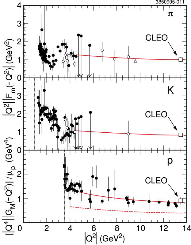
Figure 2: Compilation of the existing experimental data for the pion, kaon and proton form factors with timelike momentum transfer. The solid points are from identified $\pi^{\pm}$ and $K^{\pm}$. The open points are from unidentified $h^{\pm}$, divided into $\pi^{\pm}$ and $K^{\pm}$ according to VDM. The open triangle is from $J/\psi\rightarrow\pi^{+}\pi^{-}$, supposing it proceeds through $J/\psi\rightarrow\gamma^{*}\rightarrow\pi^{+}\pi^{-}$ only. The dashed curve is the fit to the spacelike form factor of the proton. The new CLEO points [15] are at $s=13.48\,{\rm GeV}^{2}$.

Estimates show that higher order corrections to the leading term contribution to $F_{\pi}(Q^{2})$ can constitute up to tens per sent at $Q^{2}\simeq 10\,{\rm GeV}^{2}$. Besides, one naturally expects that the asymptotic behavior is delayed in the time-like region $s=-Q^{2}>0$, in comparison with the space-like region $s=-Q^{2}<0$, so that, for instance, $|F_{\pi}(s=10\,{\rm GeV}^{2})/F_{\pi}(s=-10\,{\rm GeV}^{2})|>1$, similarly to the nucleon form factor, see fig.2 . In any case, this problem with the large value of $|s\,F_{\pi}(s=13.5\,{\rm GeV}^{2})|\simeq 1\,{\rm GeV}^{2}$ measured by CLEO [15] is much more severe for $\phi_{\pi}(x)\simeq\phi^{(asy)}(x)$, in which case the leading term contribution has to be increased $\simeq 7-8$ times to compare with the data, than for $\phi_{\pi}(x)\simeq\phi_{\pi}^{(CZ)}(x)$, where the difference is about a factor of two, see eq.(8).

The ratio $F_{K}(Q^{2})/F_{\pi}(Q^{2})$ measures the $SU(3)$ symmetry breaking effects. It was obtained in [8] that the kaon wave function $\phi_{K}(x)$ is narrower than $\phi_{\pi}(x)$. This decreases the value of the integral in eq.(2) and compensates for $f_{K}/f_{\pi}\simeq 1.2$. So, while the naive estimate looks as : $F_{K}(Q^{2})/F_{\pi}(Q^{2})=(f_{K}/f_{\pi})^{2}\simeq 1.5$,  it was predicted in [12] : $F_{K}(Q^{2})/F_{\pi}(Q^{2})\simeq 0.9$, and this agrees with the recent CLEO data at $s_{o}=13.48\,{\rm GeV}^{2}$ [15], see fig.2 :

$$s_{o}F_{K}(s_{o})=(0.84\pm 0.05\pm 0.02){\rm GeV}^{2}\,,$$

$$s_{o}F_{\pi}(s_{o})=(1.01\pm 0.11\pm 0.07){\rm GeV}^{2}\,.$$ (37)

4. The form factor $\gamma^{*}\gamma\pi^{o}.$

This form factor has been measured by CLEO [16] in the range $2\,{\rm GeV}^{2}<Q^{2}<8\,{\rm GeV}^{2}$. The measured value at $Q_{o}^{2}=8\,{\rm GeV}^{2}$ is :

$$\Phi_{\gamma\pi}(Q_{o}^{2})\equiv Q_{o}^{2}F_{\gamma\pi}(Q_{o}^{2})=(16.7\pm 2.5\pm 0.4)\cdot 10^{-2}\,{\rm GeV}.$$ (38)

From the theory side, see e.g. [17], [12] :

$$\Phi_{\gamma\pi}(Q^{2})=I_{o}\Biggl{(}1+O(\alpha_{s})+O(\Lambda^{2}_{QCD}/Q^{2})\Biggr{)},\;I_{o}=\frac{\sqrt{2}\,f_{\pi}}{3}\int_{0}^{1}\frac{dx}{x}\phi_{\pi}(x,\,{\overline{\mu}}).$$ (39)

For the asymptotic wave function $\phi_{\pi}^{asy}(x)=6x(1-x):\,I_{o}^{(asy)}=\sqrt{2}\,f_{\pi}\simeq 0.184\,{\rm GeV}.$ This is a reference point. For $Q^{2}=Q_{o}^{2}$: a) when using $\phi_{\pi}^{CZ}(x,{\overline{\mu}}=0.5\,{\rm GeV})$ in eq.(11), it gives  $I_{o}^{(CZ,1)}=(5/3)I_{o}^{(asy)}\simeq 0.3\,{\rm GeV}$ ;  b) when using $\phi_{\pi}^{CZ}(x,{\overline{\mu}}\simeq 2\,{\rm GeV}),$ it gives  $I_{o}^{(CZ,2)}\simeq(4/3)I_{o}^{(asy)}\simeq 0.25\,{\rm GeV}.$ It is seen that, unlike the charmonium decays (see eqs.(6, 7)) where the decay amplitudes differ by a factor $\sim 5$ for $\phi_{\pi}^{(asy)}$ and $\phi^{CZ}_{\pi}$, the difference here is only $\sim 50\%$. So, to infer some conclusions about the form of $\phi_{\pi}(x,\mu)$ from the CLEO results, it is of crucial importance to estimate reliably the loop and power corrections in eq.(11).

As for the perturbative loop corrections, the most advanced calculation has been performed by P. Gosdzinsky and N. Kivel [18] for $\phi_{\pi}(x)=\phi^{(asy)}(x)$. Their result (calculated in the $b_{o}\gg 1$ - approximation) looks as: $\Phi_{\gamma\pi}^{(asy)}(Q_{o}^{2})\simeq I_{o}^{(asy)}\Bigl{(}1-0.30\Bigr{)}\simeq 0.13\,{\rm GeV}$.

As for the $\sim Q^{-2}$ power correction, the value obtained by A. Khodjamirian [19] for the twist-4 two- and three-particle wave functions contribution is :  $\Delta\Phi_{\gamma\pi}(Q^{2})\simeq{\sqrt{2}}\,f_{\pi}(-3\,\delta/Q^{2})={\sqrt{2}}\,f_{\pi}(-0.6\,{\rm GeV}^{2}/Q^{2})$. It is seen that it has a typical value $\sim\pm(1\,{\rm GeV}^{2}/Q^{2})$, expected for a power correction. So, for $\phi_{\pi}(x)=\phi^{(asy)}(x)$ one has on the whole at $Q_{o}^{2}=8\,{\rm GeV}^{2}$:

$${}\Phi_{\gamma\pi}^{(asy)}(Q_{o}^{2})\simeq(1-0.30-0.075)\,I_{o}^{(asy)}=0.625\cdot 0.184\,{\rm GeV}=0.115\,{\rm GeV},$$ (40)

which looks somewhat small, see eq.(10).

As for $\phi_{CZ}(x,{\overline{\mu}})$, supposing the approach of [18] will give the relative values of loop corrections similar to those for $\phi^{(asy)}(x)$, one obtains :  a) when using $\phi_{\pi}^{CZ}(x,{\overline{\mu}}=0.5\,{\rm GeV})$ for $I_{o}$ in eq.(11), this will give :  $\Phi_{\gamma\pi}^{(CZ,1)}(Q_{o}^{2})\simeq 0.67\cdot 0.3\,{\rm GeV}=0.20\,{\rm GeV}$ ;  b) when using $\phi_{\pi}^{CZ,2}(x,{\overline{\mu}}\simeq 2\,{\rm GeV})$, this will give : $\Phi_{\gamma\pi}^{(CZ,2)}(Q_{o}^{2})\simeq 0.64\cdot 0.25\,{\rm GeV}=0.16\,{\rm GeV}\,.$ In comparison with the experimental result in eq.(10), all this is not worse, at least, than for $\phi^{(asy)}(x)$.

5. The new non-local axial anomaly.

It was claimed by D. Melikhov and B. Stech in [20] that the anomaly of the axial current is not exhausted by the standard local terms, but contains a series of additional new non-local terms:

$$\partial_{\nu}\Bigl{(}{\bar{q}}\gamma_{\nu}\gamma_{5}q\Bigr{)}=2m\,\Bigl{(}{\bar{q}}\,i\gamma_{5}\,q\Bigr{)}+Q^{2}_{q}\frac{\alpha N_{c}}{4\pi}\Bigl{(}F_{\mu\nu}F^{*}_{\mu\nu}\Bigr{)}+\frac{\alpha_{s}}{4\pi}\Bigl{(}G^{a}_{\mu\nu}G^{*\,a}_{\mu\nu}\Bigr{)}+$$

$$+eQ_{q}\,\kappa\,\frac{1}{\partial^{2}_{\nu}}\Biggl{[}\partial_{\alpha}\Bigl{(}{\bar{q}}\gamma_{\beta}\,q\Bigr{)}\,F^{*}_{\alpha\beta}\Biggr{]}+O(1/\partial^{4})\,,$$ (41)

where the constant $\kappa\neq 0$.

The explicit example considered in [20] from which the above eq.(13) has been inferred, was the form factor

$$T_{\nu}=\langle\rho^{-}(q_{2})|A_{\nu}(0)|\gamma(q_{1})\rangle\,,$$ (42)

where: $A_{\nu}={\overline{d}}\gamma_{\nu}\gamma_{5}u$  is the axial current with the momentum $p=q_{2}-q_{1}$,   $\gamma(q_{1})$ is the on-shell photon and $\rho^{-}(q_{2})$ is the $\rho^{-}$ - meson. This form factor is very similar to the form factor $\gamma^{*}\gamma\pi^{o}$ considered in the previous section.

It has been obtained in [20] that (in the chiral limit and at large $p^{2}$) the divergence of $A_{\nu}$ is non-zero, see fig.3:

$$p_{\nu}\,\langle\rho^{-}(q_{2})|A_{\nu}|\gamma(q_{1})\rangle\sim\kappa\,\frac{f_{\rho}M_{\rho}}{p^{2}}+O\Bigl{(}\frac{1}{p^{4}}\Bigr{)}\,,$$ (43)

and the constant $\kappa$ was calculated explicitly through the integral over the $\rho$ - meson wave functions (see [12] for the definitions and asymptotic forms of the $\rho$- meson wave functions,  we use here the same notations and the same asymptotic forms of these wave functions as in [20],   $\Phi(x)=3x(1-x)(2x-1)/2\,,\,\,V_{\perp}(x)=3[1+(2x-1)^{2}]/4\,,\,\,V_{A}(x)=6x(1-x)\,\,)$ :

$$\kappa=\int_{0}^{1}dx\,\Bigl{[}\,\frac{\Phi(x)-(1-x)V_{\perp}(x)}{x}+\frac{(1+x)V_{A}(x)}{4\,x^{2}}\,\Bigr{]}.$$ (44)

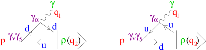
Figure 3: The diagrams for the new non-local anomaly

Substituting into eq.(16) the above explicit form of the wave functions, one obtains: $\kappa=-3/2\neq 0$. This is the main result of the paper [20].

This result looks highly surprising because the anomalous contribution originates here directly from the original light quark operators, see fig.3 . One way to make the axial anomaly ”visible”, is to use from the beginning the heavy regulator quark fields $\Psi$. Then the equations of motion are the standard ones: $\partial_{\nu}\Bigl{(}{\overline{q}}\gamma_{\nu}\gamma_{5}q+{\overline{\Psi}}\gamma_{\nu}\gamma_{5}\Psi\Bigr{)}=2m\,{\overline{q}}i\gamma_{5}q+2M\,{\overline{\Psi}}i\gamma_{5}\Psi.$ But the heavy regulator fields $\Psi$ are absent in the external low energy states. So, the regulator fields have to be contracted into the loop, from which only the gauge fields can originate. This gives the standard form of the axial anomaly. So, the light quarks do not contribute directly to the anomaly (at $m_{u,\,d}=0$ and $q_{2}^{2}\neq 0$), and the constant $\kappa$ in eq.(16) should be zero. On the other hand, the calculation of $\kappa=-3/2$ from [20] looks right, at the first sight. So, what is going wrong ?

Our answer is that the right form of eq.(16) looks really as:

$$\kappa=\lim_{\delta\rightarrow 0}\int_{0}^{1}dx\,\Bigl{[}\,\frac{\Phi(x)-(1-x)V_{\perp}(x)}{(x+\delta)}+\frac{(1+x)V_{A}(x)}{4\,(x+\delta)^{2}}\,\Bigr{]},$$ (45)

where $\delta$ is a small power correction $\sim\Lambda^{2}_{QCD}/p^{2}$, which is present in the quark propagator in fig.3 (because quarks inside the $\rho$ - meson are not strictly on-shell, but have virtualities $\sim\Lambda^{2}_{QCD}$). Calculating $\kappa$ from eq.(17) one obtains: $\kappa=0$.

The difference with [20] originates clearly from the fact that in [20] the order of $\lim_{\delta\rightarrow 0}$ and $\int^{1}_{0}dx$ was interchanged, but this is not allowed in this case.

We conclude that there is no any new non-local axial anomaly.

6. Large angle cross sections $\gamma\gamma\rightarrow\pi^{+}\pi^{-}\,,\,K^{+}K^{-}\,,\,\,K_{S}K_{S}$.

The leading contributions to the hard kernels for these amplitudes at large $s=W^{2}=(q_{1}+q_{2})^{2}$ and fixed c.m.s. angle $\theta$ were calculated first in [21] for symmetric meson wave functions, $\phi_{M}(x)=\phi_{M}(1-x)$,  and later in [22] (BC in what follows) for arbitrary wave functions. Two typical Feynman diagrams are shown in fig.4 .

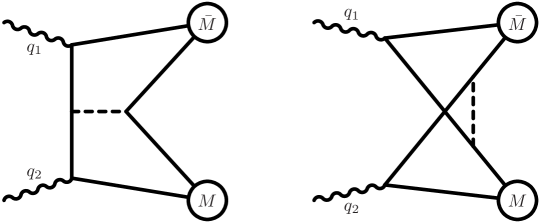
Figure 4: Two typical Feynman diagrams for the leading term hard contributions to $\gamma\gamma\rightarrow{\overline{M}}M$ , the broken line is the hard gluon exchange.

The main features of these cross sections are as follows (below we follow mainly the definite predictions from BC in [22]) .
a)   $d\sigma(\pi^{+}\pi^{-})$ can be written as :

$$\frac{s^{3}}{16\pi\alpha^{2}}\,\frac{d\sigma(\gamma\gamma\rightarrow\pi^{+}\pi^{-})}{d|\cos\theta|}\equiv\frac{|\Phi^{(eff)}_{\pi}(s,\theta)|^{2}}{\sin^{4}\theta}=\frac{|sF_{\pi}^{(lead)}(s)|^{2}}{\sin^{4}\theta}|1-\upsilon(\theta)|^{2}\,,$$ (46)

where $F_{\pi}^{(lead)}(s)$ is the leading term of the pion form factor [1] :

$$|sF^{(lead)}_{\pi}(s)|=\frac{8\pi\,{\overline{\alpha}_{s}}}{9}\,\Bigl{|}f_{\pi}\int_{0}^{1}\frac{dx}{x}\,\phi_{\pi}(x,\,{\overline{\mu}})\Bigr{|}^{2}\,.$$ (47)

While the value of $F^{(lead)}_{\pi}(s)$ is very sensitive to the form of $\phi_{\pi}(x)$, the factor $\upsilon(\theta)$, as emphasized in [21], is nearly independent on the form of $\phi_{\pi}(x)$, and depends only weakly on $\theta$. Numerically, $\upsilon(\theta)\simeq 0.12$.

The recent data from the Belle collaboration [23] for $(\pi^{+}\pi^{-})$ and $(K^{+}K^{-})$ agree with $\sim 1/\sin^{4}\theta$ dependence at $W\geq 3\,{\rm GeV}$, while the angular distribution is somewhat more steep at lower energies. The energy dependence at $2.4\,{\rm GeV}<W<4.1\,{\rm GeV}$ was fitted in [23] as: $\sigma_{o}(\pi^{+}\pi^{-})=\int_{0}^{0.6}dc(d\sigma/d|c|)\sim W^{-n}\,,\,\,\,n=(7.9\pm 0.4\pm 1.5)$ for $(\pi^{+}\pi^{-})$, and $n=(7.3\pm 0.3\pm 1.5)$ for $(K^{+}K^{-})$. The overall value $n\simeq 6$ is also acceptable however, see fig.5 . As for the absolute normalization, the $(\pi^{+}\pi^{-})$ data are fitted in [23] to the eq.(18) with : $|\Phi_{\pi}^{(eff)}(s,\theta)|=(0.503\pm 0.007\pm 0.035)\,{\rm GeV}^{2}$.   This value can be compared with  : $0.88\cdot|sF_{\pi}^{(CZ)}(s)|\simeq 0.4\,{\rm GeV}^{2}$ for $\phi_{\pi}^{(CZ)}(x,\mu_{o})$, and $0.88\cdot|sF_{\pi}^{(asy)}(s)|\simeq 0.12\,{\rm GeV}^{2}$ for $\phi^{(asy)}(x).$ It is seen that the wide pion wave function $\phi_{\pi}^{(CZ)}(x)$ is preferable, while $\phi^{(asy)}(x)$ gives the cross section which is $\simeq 15$ times smaller than data. It seems impossible that, at energies $s=10-15\,{\rm GeV}^{2}$, higher loop or power corrections can cure so large difference.

b)   The SU(3)-symmetry breaking, $d\sigma(K^{+}K^{-})\neq d\sigma(\pi^{+}\pi^{-}),$ originates not only from different meson couplings, $f_{K}\neq f_{\pi}$, but also from symmetry breaking effects in normalized meson wave functions, $\phi_{K}(x)\neq\phi_{\pi}(x)$. These two effects tend to cancel each other. So, instead of the naive prediction $\simeq(f_{K}/f_{\pi})^{4}\simeq 2.3$ from [21], the prediction of BC for this ratio is close to unity, and this agrees with the recent data from Belle [23]:

$$\frac{\sigma_{o}(\gamma\gamma\rightarrow K^{+}K^{-})}{\sigma_{o}(\gamma\gamma\rightarrow\pi^{+}\pi^{-})}=\left\{\begin{array}[c]{ll}\displaystyle(f_{K}/f_{\pi})^{4}\simeq 2.3\scriptstyle&\begin{array}[c]{l}\rm{Brodsky,\,Lepage}\,\,\cite[cite]{[\@@bibref{}{BL2}{}{}]}\end{array}\\ &\\ \hline\cr&\\ \simeq 1.06&\begin{array}[c]{l}\rm{Benayoun,\,Chernyak}\,\,\cite[cite]{[\@@bibref{}{Maurice}{}{}]}\end{array}\\ &\\ \hline\cr&\\ (0.89\pm 0.04\pm 0.15)\quad{\rm Belle}-2004\,\,\,\cite[cite]{[\@@bibref{}{Belle1}{}{}]}\end{array}\right.$$ (57)

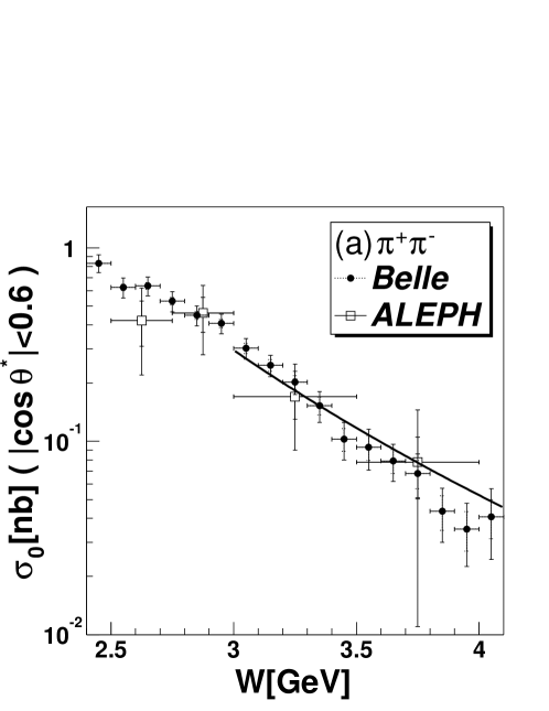
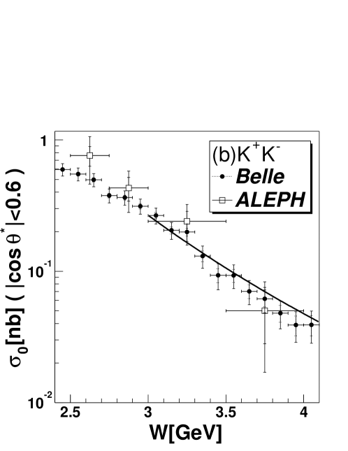
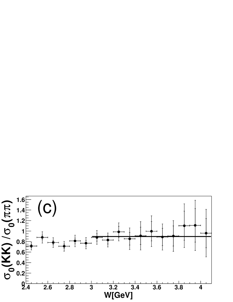
Figure 5: The cross sections $\sigma_{o}=\int d\cos\theta\,(d\sigma/d\cos\theta)$ ,  integrated over the c.m. angular region $|\cos\theta|<0.6\,,\,\,$ for a) $\,\,\gamma\gamma\ \rightarrow\pi^{+}\pi^{-}\,\,$, b) $\,\,\gamma\gamma\rightarrow K^{+}K^{-}\,\,,$  together with a $W^{-6}$ dependence line ;   c) the cross section ratio, the solid line is the result of the fit for the data above $3\,{\rm GeV}$ ,   the errors indicated by short ticks are statistical only.

c)   The leading terms in cross sections for neutral particles are much smaller than for charged ones. For instance, it was obtained by BC that the ratio $d\sigma^{(lead)}(\pi^{o}\pi^{o})/d\sigma^{(lead)}(\pi^{+}\pi^{-})$ varies from $\simeq 0.07$ at $\cos\theta=0$ to $\simeq 0.04$ at $\cos\theta=0.6$. Besides, it was obtained therein for the ratio : $({\overline{K}}^{o}K^{o})^{(lead)}/(\pi^{o}\pi^{o})^{(lead)}\simeq 1.3\cdot(4/25)\simeq 0.21\,.$ So, for instance, one obtains for cross sections $\sigma_{o}^{(lead)}$ integrated over $0\leq|\cos\theta|\leq 0.6$ for charged particles and over $0\leq\cos\theta\leq 0.6$ for neutral ones  :   $\sigma_{o}^{(lead)}(K_{S}K_{S})/\sigma_{o}^{(lead)}(K^{+}K^{-})\simeq 0.005\,.$

It is seen that the leading contribution to $\sigma_{o}(K_{S}K_{S})$ is very small. This implies that, unlike to the case $\sigma_{o}(K^{+}K^{-})$, it is not yet dominant at present energies $W^{2}<16\,GeV$. In other words, the amplitude $A(\gamma\gamma\rightarrow K_{S}K_{S})=(a(s,\theta)+b(s,\theta))$ is dominated by the non-leading term $b(s,\theta)\sim g(\theta)/s^{2}$, while the formally leading term $a(s,\theta)\sim C_{o}f_{BC}(\theta)/s$ has so small coefficient $C_{o}$ that $|b(s,\theta)|>|a(s,\theta)|$ at, say, $W^{2}<12\,GeV^{2}$. So, it has no meaning to compare the leading term prediction of BC (i.e. $d\sigma(K_{S}K_{S})/d\cos\theta\sim|a(s,\theta)|^{2}/s\sim|f_{BC}(\theta)|^{2}/W^{6}$ at $s\rightarrow\infty$) for the energy and angular dependence of $d\sigma(K_{S}K_{S})$ with the recent data from Belle [24]. Really, the only QCD prediction for $6\,GeV^{2}<W^{2}<12\,GeV^{2}$ is the energy dependence: $d\sigma(K_{S}K_{S})/d\cos\theta\sim|b(s,\theta)|^{2}/s\sim|g(\theta)|^{2}/W^{10}$, while the angular dependence $|g(\theta)|^{2}$ and the absolute normalization are unknown. This energy dependence agrees with [24], see fig.7 .

The hand-bag model [25] (DKV in what follows) is a part of a general ideology which claims that present day energies are insufficient for the leading terms QCD to be the main ones. Instead, the soft nonperturbative contributions are supposed to dominate the amplitudes. The handbag model represents applications of this ideology to description of $d\sigma(\gamma\gamma\rightarrow{\overline{M}}M)$. It assumes that the above described hard contributions really dominate at very high energies only, while the main contributions at present energies originate from the fig.6a diagram.

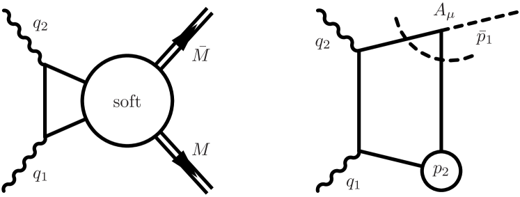
Figure 6: a) the overall picture of the handbag contribution,  b) the lowest order Feynman diagram for the light cone sum rule

Here, two photons interact with the same quark only, and these ”active” ${\overline{q}}q$-quarks carry nearly the whole meson momenta, while the additional ”passive” ${\overline{q}^{\prime}}q^{\prime}$ quarks are ”wee partons” which are picked out from the vacuum by soft non-perturbative interactions. It was obtained by DKV that the angular dependence of amplitudes is $\sim 1/\sin^{2}\theta$ for all charged and neutral pions or kaons, while the energy dependence is not predicted and is described by some soft form factors $R_{M}(s),$ which are then fitted to the data. Because the ”passive” quarks are picked out from the vacuum by soft non-perturbative forces, these soft form factors are power suppressed at sufficiently large $s\,:R_{M}(s)\leq 1/s^{2}\,,\,$ in comparison with the leading meson form factors, $F_{M}(s)\sim 1/s\,$.

Some specific predictions of the handbag model look as :
$\sigma_{o}(\pi^{o}\pi^{o})/\sigma_{o}(\pi^{-}\pi^{-})=1/2$,  and

$$\frac{\sigma_{o}(K_{S}K_{S})}{\sigma_{o}(K^{+}K^{-})}=\frac{1}{2}\Biggl{|}\frac{e^{2}_{s}\,R_{s\rightarrow d}(s)+e_{d}^{2}\,R_{d\rightarrow s}(s)}{e_{u}^{2}\,R_{u\rightarrow s}(s)+e_{s}^{2}\,R_{s\rightarrow u}}\Biggr{|}^{2}=\frac{2}{25}\Biggl{|}\frac{1-\Delta}{1-\frac{8}{5}\Delta}\Biggr{|}^{2}>0.08.$$ (58)

Here, $e_{u}=2/3,\,\,e_{d}=e_{s}=-1/3$ are the quark charges, while the form factor $R_{u\rightarrow s}(s)$ corresponds to the active $u$-quark and passive $s$-quark, etc. It seems clear that it is harder for soft interactions with the scale $\sim\Lambda_{QCD}$ to pick out from the vacuum the heavier ${\overline{s}}s$-pair, than the light ${\overline{u}}u$-  or ${\overline{d}}d$-pairs. So :   $R_{u\rightarrow s}(s)/R_{s\rightarrow u}(s)\equiv(1-2\Delta)\,,\,\,\Delta>0$.  ( The same inequality $\Delta>0$ follows from the fact that the heavier s-quark carries, on the average, the larger fraction, $\langle x_{s}\rangle\,>\,0.5,$ of the K-meson momentum). Therefore, the handbag model predicts that the number $2/25=0.080$ is the lower bound in eq.(20).

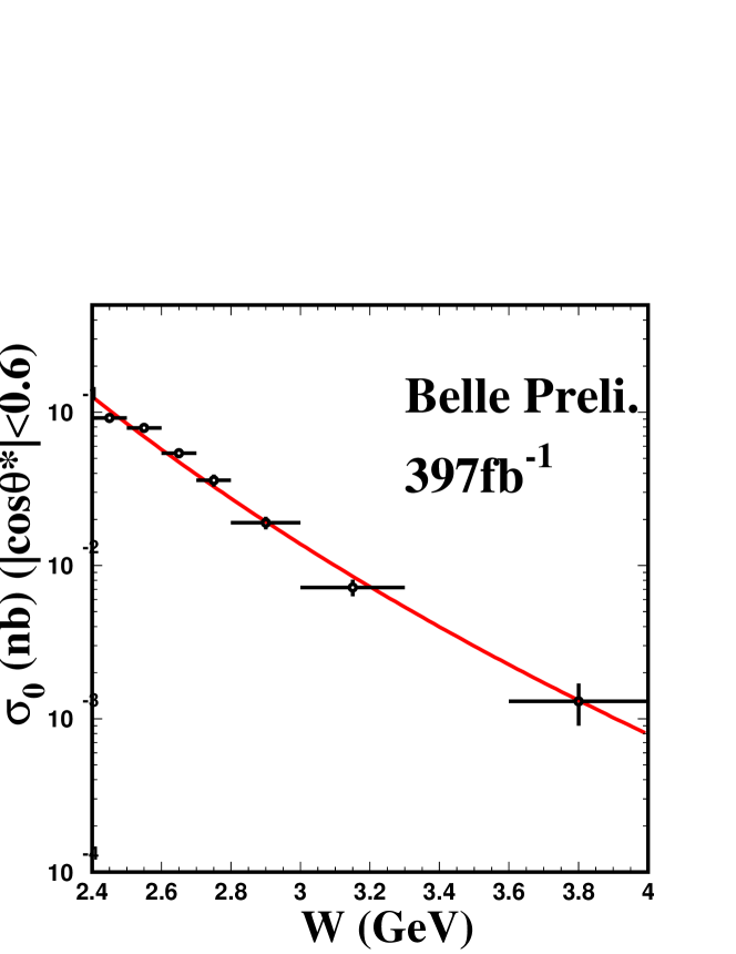
Figure 7: The measured energy dependence of $\sigma_{o}(K_{S}K_{S})$ ,  [24]. The solid line is $\,\sim W^{-k},\,\,k\simeq 10$.

The cross section $d\sigma(K_{S}K_{S})/d\cos\theta$ has been measured recently by the Belle collaboration [24]. The energy dependence at $2.4\,{\rm GeV}<W<4.0\,{\rm GeV}$ was found to be :  $\sigma_{o}(K_{S}K_{S})\sim W^{-k}\,,\,k=(9.93\pm 0.4)$, see fig.7 . As for the angular distribution, it is consisted with $d\sigma(K_{S}K_{S})/d\cos\theta\sim 1/(W^{10}\sin^{4}\theta)$, [24]. The measured ratio $(K_{S}K_{S})/(K^{+}K^{-})$ decreases strongly with increasing energy, and becomes smaller than the lower bound $0.080$ in eq.(20) at $W\simeq 2.8\,{\rm GeV}$. This is in contradiction with the hand-bag model predictions. 

Moreover, the recent explicit calculation of the hand-bag diagrams in [26] using the method of the light cone sum rules [27] [28], see fig.6b , shows that for all channels, $\pi^{+}\pi^{-}\,,\,K^{+}K^{-}$ and $K_{S}K_{S}$ : a) the energy dependence of the handbag form factors $R_{M}(s)$ is $\sim(s_{o}/s)^{2}$ already in the energy interval $2.5\,{\rm GeV}<W=\sqrt{s}<4\,{\rm GeV}$ where the experiments have been done, and so this disagrees with the data on $\sigma_{o}(\pi^{+}\pi^{-})$ and $\sigma_{O}(K^{+}K^{-})$ ;  b) all handbag amplitudes do not depend on the scattering angle $\theta$ (in contradiction with the DKV results)  :

$$\frac{d\sigma^{handbag}({\overline{M}}M)}{d\cos\theta}\sim\frac{|R_{M}(s)|^{2}}{s}\sim\frac{const}{W^{10}}\,,$$ (59)

and this disagrees with the data which show $(\sim 1/\sin^{4}\theta)$  dependence ; c) and finally, the absolute values of all three cross sections predicted by the hanbag model are much smaller than their experimental values.

The conclusion for this section is that the leading term QCD predictions for $\gamma\gamma\rightarrow{\overline{M}}M$ are in a reasonable agreement with the data (but only for the wide pion and kaon wave functions, like $\phi_{\pi,K}^{(CZ)}(x)$), while the hand-bag model contradicts the data in all respects : the energy dependence, the angular distribution and the absolute normalization.

References

[1]
V.L. Chernyak, A.R. Zhitnitsky, JETP Lett. 25 (1977) 510
[11]
A.V. Radyushkin, Talk given at the Workshop ”Continuous Advances in QCD”, University of
Minnesota, Minneapolis, Feb. 18-20, 1994. In Proc. ”Continuous advances in QCD”, pp. 238-248;
Preprint CEBAF-TH-94-13; hep-ph/9406237
[22]
M. Benayoun, V.L. Chernyak, Nucl. Phys. B329 (1990) 285
[23]
H. Nakazawa et. al. (Belle Collaboration), Phys. Lett. B615
(2005) 39 ; hep-ex/0412058
[24]
W.T. Chen (Belle collaboration), ”Measurements of production and
charmonium studies in two-photon processes at Belle”,
Talk at the Int. Conf.
”Photon-2005”, September 3, 2005, Warsaw and Kazimierz, Poland
[25]
M. Diehl, P. Kroll, C. Vogt, Phys. Lett. B532 (2002) 99 ;
hep-ph/0112274