Constraining pre Big–Bang–Nucleosynthesis Expansion using Cosmic Antiprotons

Abstract

A host of dark energy models and non–standard cosmologies predict an enhanced Hubble rate in the early Universe: perfectly viable models, which satisfy Big Bang Nucleosynthesis (BBN), cosmic microwave background and general relativity tests, may nevertheless lead to enhancements of the Hubble rate up to many orders of magnitude. In this paper we show that strong bounds on the pre–BBN evolution of the Universe may be derived, under the assumption that dark matter is a thermal relic, by combining the dark matter relic density bound with constraints coming from the production of cosmic–ray antiprotons by dark matter annihilation in the Galaxy. The limits we derive can be sizable and apply to the Hubble rate around the temperature of dark matter decoupling. For dark matter masses lighter than 100 GeV, the bound on the Hubble–rate enhancement ranges from a factor of a few to a factor of 30, depending on the actual cosmological model, while for a mass of 500 GeV the bound falls in the range 50–500. Uncertainties in the derivation of the bounds and situations where the bounds become looser are discussed. We finally discuss how these limits apply to some specific realizations of non–standard cosmologies: a scalar–tensor gravity model, kination models and a Randall–Sundrum D–brane model.

I Introduction

Current cosmological and astrophysical observations clearly show that our Universe is dominated by two unknown and exotic components, dark matter and dark energy, whose energy densities are measured to fall in the following ranges (at $2\sigma$ C.L.) omegalimits :

$$0.092\leq\Omega_{\rm CDM}h^{2}\leq 0.124$$ (1)

for the cold dark matter (CDM) component, responsible of structure formations and galactic and extragalactic dynamics, and:

$$0.30\leq\Omega_{\rm DE}h^{2}\leq 0.46$$ (2)

for the unclustered dark energy component, which is responsible of the current accelerated expansion of the Universe. (As usual $\Omega$ denotes the ratio between the mean density and the critical density and $h$ is the Hubble constant in units of $100\ \textrm{km}\ \textrm{s}^{-1}\ \textrm{Mpc}^{-1}$.)

The nature of both components is unknown. A common and appealing possibility is that dark matter is composed by elementary particles which decoupled from the thermal plasma in the early Universe. The dark energy component poses more serious problems: a possibility is that it is due to the presence of a scalar field, whose cosmological dynamics allows it to become the dominant component of the Universe just recently in the evolutionary history of the Universe. Most of the dark energy models predict that the expansion rate of the Universe may have been different from the one predicted by the standard Friedman–Robertson–Walker (FRW) model at very early stages. Not only dark energy models, but also other cosmological models, can predict an enhancement of the Hubble rate note on reduction . If this occurs around the time when the dark matter particles decouple from the thermal bath, the change in the Hubble rate may leave its imprint on the relic abundance of the dark matter. This has been discussed in details in dark energy models based on scalar–tensor gravity scalartensorrelic and in quintessence models with a kination phase Salati ; Rosati ; profumoullio ; Pallis and for anisotropic expansion and other models of modified expansion Barrow ; kamionkowskiturner . This effect implies that the basic CDM properties may depend on the specific cosmological model. Thus, information on the CDM particles may be used to constrain cosmological models and vice versa. In this paper we will exploit this connection between the dark matter and the expansion rate in order to derive bounds on cosmological models from observational data related to the dark matter particles. We emphasize that the effects we are going to study do not arise because of a direct coupling between dark energy and dark matter: they are instead due to the effect induced by the dark energy model (or other models with enhanced expansion) on the decoupling of the dark matter particle.

We will consider a generic Weakly Interacting Massive Particle (WIMP) as candidate of cold dark matter. For the cosmological model we consider models that lead to an enhancement of the Hubble expansion rate in the early Universe as compared to the rate in standard cosmology, like those in Refs. scalartensorrelic ; Salati ; Randall . In order to be general in our analysis, we will consider a suitable parametrization of the enhancement of the Hubble rate in the early Universe. As specific examples we will then relate our parametrization to scalar–tensor gravity (ST) models scalartensorrelic , to models with a kination phase Salati and to a Randall–Sundrum D–brane model Randall .

The enhancement of the Hubble expansion rate in the early Universe can affect phenomena that are sensitive to the exact time at which they occur. This is the case for the freeze–out of a WIMP. The enhanced Hubble rate causes an enhanced WIMP dilution. The WIMP annihilation rate therefore cannot keep up with the expansion as long as in the standard case. Consequently, the WIMP freezes out earlier in this kind of non–standard cosmologies, leading to a higher relic abundance. The enhancement of the WIMP relic abundance can be very dramatic, up to a few orders of magnitude scalartensorrelic ; Salati . The requirement that the WIMP is the dominant dark matter component, i.e. that its relic abundance satisfies the bound of Eq. (1), implies that the properties of the successful WIMP are dramatically changed with respect to the standard FRW case. Since the dark matter relic abundance, apart from the expansion, mainly depends on the WIMP mass and annihilation cross section, we can say that the cosmological model has left its fingerprint on the dark matter. A fingerprint which could turn out to be one of the most important signatures of these dark energy and other cosmological models.

In fact the WIMPs that in the modified scenario have the correct relic density possess a higher annihilation cross section than do WIMPs selected by standard cosmology. This means that indirect detection signals are favoured in the modified scenario. In particular, it has been shown that the antiproton component in cosmic rays is a powerfull tool to constrain dark matter properties, even though it is affected by large astrophysical uncertainties pb . In Ref. pbarlim combined limits in the astrophysical–WIMP parameter space have been derived and it has been shown that antiprotons can powerfully set bounds on WIMPs in the tens–hundreds of GeV range. We are going to apply the same argument here, from which we will be able to derive constraints on the cosmological models with enhanced Hubble expansion. We will show that the constraints on dark matter coming from antiproton indirect searches strongly constrain the cosmological models with enhanced Hubble rate in the early Universe. When one studies a specific cosmological model, the model can be constrained by a number of relevant observables, related to e.g. Big Bang Nucleosynthesis (BBN) Cyburt , Cosmic Microwave Background (CMB), Large Scale structure and Supernovae Wang ; Zhao , weak lensing Albert and General Relativity tests Cassini . We will show that the antiproton bound, under suitable condition, may result in even stronger limits.

In Section II we discuss our parametrization of the enhanced Hubble rate, and in Section III we show its connection to specific cosmological models. In Section IV we discuss the relic density calculation in modified cosmology, for which some useful analytical approximations are given in Appendix A. Section V deals with the cosmic antiproton signal and the bounds on the dark matter. In Section VI we then derive the constraints on the cosmological models. Section VII translates our bounds to some specific cosmological models, namely scalar–tensor cosmology, kination models and Randal–Sundrum D–brane cosmology. Finally, in Section VIII we summarize our main results.

II The Hubble enhancement function

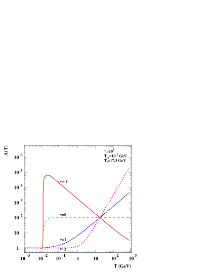
Figure 1: The Hubble rate enhancement function $A(T)$ as a function of the temperature. Notice that time is running from right to left. The solid red line has a slope parameter $\nu=-1$, the dashed green line $\nu=0$, the dash-dotted blue $\nu=1$ and the dotted purple line has $\nu=2$. For all the curves we have chosen $\eta=10^{2}$ and $T_{\textrm{re}}=10^{-2}$ GeV. The freeze out temperature of the relic WIMP has been fixed to $T_{\textrm{f}}=17.3$ GeV (a case which refers, e.g., to a particle with mass of 500 GeV and annihilation cross section $\langle\sigma_{\textrm{ann}}v\rangle=10^{-7}\,\textrm{GeV}^{-2}$).

Let us consider a class of cosmological models that posses a Hubble rate $H$ in the early Universe enhanced with respect to its value in standard cosmology $H_{\textrm{std}}$. We parametrize this enhancement by means of a function $A(T)$:

$$H = A(T)H_{\textrm{{std}}}\qquad\qquad\textrm{at early times}$$ (3)

$$H = H_{\textrm{{std}}}\qquad\qquad\qquad\,\textrm{at later~{}times}$$ (4)

This situation occurs e.g. in scalar-tensor gravity models and in models with a kination phase. Also some models with extra dimensions lead to an enhanced Hubble rate. We will review some of these examples in the next Section to show that they can all be covered by the following parametrization of the enhancement function $A(T)$:

$$A(T)=1+\eta\left(\frac{T}{T_{\textrm{f}}}\right)^{\nu}\tanh\left(\frac{T-T_{\textrm{re}}}{T_{\textrm{re}}}\right)$$ (5)

for temperatures $T>T_{\textrm{re}}$ and $A(T)=1$ for $T\leq T_{\textrm{re}}$. By $T_{\textrm{re}}$ we denote the temperature at which the Hubble rate “re–enters” the standard rate and by $T_{f}$ a reference temperature, which we specify below. Clearly the Hubble parameter has to approach the General Relativity (GR) case at some epoch $T_{\textrm{re}}\gtrsim 1\ \textrm{MeV}$, in order not to spoil the successful predictions of Big Bang Nucleosynthesis and the formation of the Cosmic Microwave Background Radiation (CMB). These two key events in the history of the Universe are typically among the major constraints on DE theories.

In fig. 1 we show $A(T)$ for $\eta=100$, $T_{\textrm{re}}=10^{-2}$ GeV and four different values of the exponent $\nu$, which we will use throughout the paper as reference points in our analysis. The figure shows that at the temperature $T_{\textrm{f}}$ (which here is $T_{f}\gg T_{\textrm{re}}$) all curves take the same value $\eta$ (since $\eta\gg 1$). In our analysis, we will take $T_{\textrm{f}}$ as the temperature at which the WIMP freezes out in standard cosmology. In a situation like the one shown in the figure, the parameter $\eta$ gets the meaning of enhancement factor of the Hubble rate at the time of WIMP freeze–out.

The slope of the curve around $T_{\textrm{f}}$ is mostly determined by the exponent $\nu$. We arbitrarily use in Eq. (5) a hyperbolic tangent to assure that all curves approach unity as a continuos function when the temperature of the Universe approaches $T_{\textrm{re}}$. However, for analytic approximations that may help to understand our numerical results, a sharp jump to the standard case at $T=T_{\textrm{re}}$ is appropriate. Changes in the slope of the re–entering phase will be briefly discussed in Sect. VI.3.

III Cosmological models with a modified expansion rate

In this section we present a short list of interesting cosmological models which lead to an enhanced expansion rate as compared to the standard Friedman–Robertson–Walker (FRW) model based on General Relativity.

III.1 Scalar–tensor theories

In a scalar–tensor theory of gravity both a metrical tensor $g_{\mu\nu}$ and a scalar field $\varphi$ are involved in the description of the gravitational interaction Damour . Because of this additional scalar degree of freedom, the Universe expands differently compared to a standard FRW solution of the Einstein gravity equations scalartensorrelic . This class of theories can be formulated in different frames related to each other by a Weyl re–scaling of the metric Esposito . As pointed out in Ref. Dicke , a frame transformation amounts in a change of units and therefore the physical results cannot depend on the frame. A frame-independent formulation of the scalar–tensor cosmology is given in Pietroni . In order to deal with scalar field-independent masses and couplings, in the language of scalar–tensor theories this means that we stay in the Jordan frame. This was our approach in the calculation of the effects induced on the WIMP decoupling in scalar–tensor theories in Ref. scalartensorrelic .

The ratio between the Jordan frame expansion rate and the standard General Relativity expansion rate is given by scalartensorrelic :

$$\frac{H^{2}}{H_{std}^{2}}=A^{2}(\varphi)\frac{\left[1+\alpha(\varphi)\varphi^{\prime}\right]^{2}}{1-(\varphi^{\prime})^{2}/6}$$ (6)

where $\alpha(\varphi)=d\log A(\varphi)/d\varphi$, $A(\varphi)$ is the Weyl factor relating the Jordan and Einstein frame and a prime denotes derivation with respect to the logarithm of the scale factor.

To find a general correspondence between our parametrization in Eq. (5) and a scalar–tensor behaviour of the expansion rate is quite difficult. This is due to the fact that the scaling of the ratio in Eq. (6) is deeply related with the cosmological dynamics of the scalar field. However, as shown in a specific example in Ref. scalartensorrelic , a numerical solution of the scaling behavior of Eq. (6) can be translated in terms of our parametrization. In the simplest case of a slowly varying scalar field ($\varphi^{\prime}\simeq 0$) we have $H=A(\varphi)H_{\textrm{std}}$, and in the specific example of scalartensorrelic we have $A(\varphi)=A(\varphi(T_{\textrm{f}}))(T/T_{\textrm{f}})^{-0.82}$. In terms of our parametrization, this example has $\eta=A(\varphi(T_{\textrm{f}}))$ and $\nu=-0.82$. Fig. 6 of Ref. scalartensorrelic shows that the enhancement of the Hubble rate around the WIMP freeze–out may be quite sizeable, up to factors of $10^{4}$. We remind that the model studied in Ref. scalartensorrelic was a perfectly viable scalar–tensor model, since it evaded all experimental constraints from BBN, CMB and gravitational probe limits, like the Cassini mission Cassini . The enhanced Hubble rate reflects in an anticipated WIMP decoupling, with an ensuing larger relic abundance. Ref. scalartensorrelic showed that for such a fast re–entering of the Hubble rate on its GR behaviour, it may be possible that the already–decoupled WIMPs start a brief phase of re–annihilation, due to the fact that they are still over–abundant and therefore their annihilation rate is larger than the GR Hubble rate. This phenomenon has the consequence of reducing the WIMP relic abundance with respect to the value it would have had without re–annihilation. Nevertheless, the outcome of this scalar–tensor model is that the WIMP current abundance may be larger that the GR one by up to 2-3 orders of magnitude. This result would then be even stronger if a re–annihilation phase does not occur, due to a slower re–entering of the Hubble rate to GR. Summarizing: perfectly viable scalar–tensor models from the point of view of cosmological and astrophysical observations, may predict a strongly enhanced WIMP relic abundance for a give candidate. This was our original motivation to try to set additional limits on these cosmologies by means of observables related to the dark matter sector, namely the antiproton indirect–detection signal, as it will be described in the next Sections. However, our discussion may be applied also to other cosmological scenarios with enhanced early Hubble rate, like the following two relevant cases.

III.2 Kination

A kination is a period in which the total energy density of the Universe is dominated by the kinetic term of a scalar field. A phase of kination is generically expected in quintessence models based on tracking solutions for the scalar field, Ref. Steinhardt . When the scalar potential $V(\Phi)$ is negligible compared to the kinetic energy of the scalar field, the total energy density in the scalar field, $\rho_{\Phi}$, scales like $\sim a^{-6}$ (where $a$ is the scale factor of the Universe). This means that during kination $H^{2}\propto\rho_{\textrm{tot}}\simeq\rho_{\Phi}\propto a^{-6}$. More precisely, the ratio between the expansion rate $H$ during a kination period and the standard expansion rate $H_{std}$ is given by:

$$\frac{H^{2}}{H^{2}_{std}}=1+\frac{\rho_{\Phi}}{\rho_{r}}\,,$$ (7)

where $\rho_{\Phi}/\rho_{r}$ can be written as Salati

$$\frac{\rho_{\Phi}}{\rho_{r}}=\eta_{\Phi}\left[\frac{h(T)}{h(T_{\textrm{f}})}\right]^{2}\frac{g(T_{\textrm{f}})}{g(T)}\left(\frac{T}{T_{\textrm{f}}}\right)^{2}\simeq\eta_{\Phi}\left(\frac{T}{T_{\textrm{f}}}\right)^{2}$$ (8)

with $\eta_{\Phi}=\rho_{\Phi}(T_{\textrm{f}})/\rho_{r}(T_{\textrm{f}})$ and $h_{\textrm{eff}}$ and $g_{\textrm{eff}}$ respectively the entropy–density and energy–density effective degrees of freedom. The approximation in Eq. (8) is justified only in a range of temperatures where $h_{\textrm{eff}}$ and $g_{\textrm{eff}}$ do not change considerably with respect to their value at $T_{\textrm{f}}$.

From Eq. (7) and (8) we see that a kination model can be approximated by our parametrization once the following values for the parameters are chosen: $\nu=1$ and $\eta=\sqrt{\eta_{\Phi}}$.

III.3 Extra Dimensions

We refer to the RSII model Randall . In this model a single 3–brane is embedded in a five dimensional bulk with a negative five dimensional cosmological constant. Unlike other Extra Dimension models, here the fifth dimension is not compact and no orbifold boundary conditions are imposed. Moreover, the five–dimensional metric is not factorizable and an exponential function of the fifth coordinate multiplies the four dimensional metric. With this set up, a Kaluza Klein (KK) reduction of the five dimensional gravitational excitations gives rise to a spectrum with a zero mode (the standard four–dimensional graviton) localized in the extra dimension and a continuum of massive KK modes weakly coupled to the low energy states on the brane. Due to the fact that the four–dimensional gravitons can propagate in a confined region of the fifth dimension and since at low energy the massive KK modes are only weakly coupled, the theory is not in contrast with experimental gravity even if the volume of the extra dimension is infinite. The Einstein equation on the 3-brane are studied in Ref. Shiromizu and the cosmology of such a model is carefully investigated in Ref. Durrer . In particular it has been shown that the ratio between the expansion rate $H$ of such a model and the expansion rate $H_{std}$ of standard cosmology is given by:

$$\frac{H^{2}}{H^{2}_{std}}=1+\frac{\rho}{2\lambda}$$ (9)

where $\lambda$ is the tension on the brane and $\rho$ the energy density on the brane. When the total energy density $\rho$ equals the radiation energy density $\rho_{r}$ we have:

$$\frac{H}{H_{std}}\simeq\sqrt{\frac{\rho_{r}(T_{\textrm{f}})}{2\lambda}}\left(\frac{T}{T_{\textrm{f}}}\right)^{2}$$ (10)

Comparing this expression with Eq. (5), we see that such a model is described by our parametrization with the values of the parameters $\nu=2$ and $\eta=\sqrt{\rho_{r}(T_{\textrm{f}})/(2\lambda)}$.

IV The relic density calculation

In this section we will briefly discuss how a cosmological model with enhanced Hubble rate affects the relic abundance of WIMP dark matter. This effect was studied in details in Ref. scalartensorrelic for the scalar–tensor case and in Refs. Salati ; Rosati ; profumoullio ; Pallis for the kination case. See also Refs. Barrow ; kamionkowskiturner for anisotropic expansion and other models of modified expansion.

The evolution of the WIMP number density $n$ as a function of cosmological time $t$ is described by the standard Boltzmann equation, the only difference being that the standard Hubble parameter $H_{\textrm{{std}}}(T)$ is now replaced by the modified Hubble rate, $H(T)=A(T)H_{\textrm{{std}}}(T)$:

$$\frac{dn}{dt}=-3Hn-\langle\sigma_{\textrm{ann}}v\rangle(n^{2}-n_{\textrm{eq}}^{2})$$ (11)

where $\langle\sigma_{\textrm{ann}}v\rangle$ is the usual thermally averaged value of the WIMP annihilation cross section times the relative velocity. The modification of the Hubble rate can be rephrased as a change in the effective number of degrees of freedom from $g_{\textrm{eff}}(T)$ to $A^{2}(T)g_{\textrm{eff}}(T)$. The Boltzmann equation is more conveniently solved by rewriting it in terms of the comoving abundance $Y=n/s$ where $s$ is the entropy density $s=(2\pi^{2}/45)h(T)T^{3}$ and studying the evolution as a function of the temperature $T$:

$$\frac{dY}{dx}=-\frac{1}{x}\frac{s}{H}\langle\sigma_{\textrm{ann}}v\rangle(Y^{2}-Y^{2}_{\textrm{eq}})$$ (12)

where $x=m_{\chi}/T$. In our analysis we solve the Boltzmann equation Eq. (12) numerically down to the current value of the comoving abundance $Y_{0}$. The WIMP relic abundance is then simply:

$$\Omega_{\chi}h^{2}=\frac{m_{\chi}s_{0}Y_{0}}{\rho_{c}}$$ (13)

where $s_{0}$ and $\rho_{c}$ are the current values for the entropy density and the critical mass–density of the Universe. In order to get some insight in our numerical results, we report in Appendix A some useful analytical approximations which are valid for large enhancements and re–entering temperature (much) lower than the temperature at which decoupling occurs. Notice that in our definition of the function $A(T)$ in Eq. (5), we use as a normalization temperature the freeze–out temperature obtained in standard cosmology and defined in Appendix A. We report it here for convenience:

$$x_{\textrm{f}}=\ln\left[0.038\,m_{\textrm{pl}}\,g\,m_{\chi}{\langle\sigma_{\textrm{ann}}v\rangle_{T_{\textrm{f}}}x_{\textrm{f}}^{-1/2}}{g^{-1/2}_{\textrm{eff}}(x_{\textrm{f}})}\right]$$ (14)

The effect of the enhanced Hubble rate on the WIMP relic density can be very important. As was found in Ref. scalartensorrelic , and as we are also going to see later in this paper, the relic density can be up to few orders of magnitude larger in the modified scenario as compared to the standard case. From combined cosmological observations we have the very stringent bound of Eq. (1) for the cold dark matter density. This means that the WIMP candidates selected in the case of enhanced Hubble rate will be vastly different (i.e. have different values of their relevant parameters, like mass and couplings) from the WIMPs that fit into the standard cosmology picture. The cosmological model has, in other words, left its signature on the dark matter. A signature which might turn out to give valuable clues.

Not only can we say that the WIMPs selected in the standard and modified cases are different, we are also able to say something general about the difference of their phenomenology. This builds on the fact that the standard WIMP relic abundance in general is approximately inversely proportional to the WIMP annihilation cross section. Analytically one finds (see Appendix A) the well–known behaviour:

$$\Omega_{\chi}h^{2}\sim\frac{1}{\langle\sigma_{\rm ann}v\rangle_{\rm int}}$$ (15)

where $\langle\sigma_{\rm ann}v\rangle_{\rm int}$ is the following integration of the thermal annihilation cross–section:

$$\langle\sigma_{\rm ann}v\rangle_{\rm int}\equiv\frac{1}{{\cal G}(x_{\rm f})}\int_{x_{\rm f}}^{\infty}\frac{{\cal G}(x)\,\langle\sigma_{\textrm{ann}}v\rangle}{A(x)\,x^{2}}\,dx$$ (16)

The WIMPs that fulfill the relic density constraint of Eq. (1) when calculated with the enhanced Hubble rate, would have a much lower density when recalculated in standard cosmology. From Eqs. (15,16) this then means that these WIMPs have a higher annihilation cross section than WIMPs that satisfy the relic density constraints when calculated with the standard Hubble expansion. A high WIMP annihilation cross section in the early Universe does in general mean that also the current WIMP annihilation rate in the Galaxy is high . The WIMP candidates selected by the models of enhanced expansion rate are therefore in general more suitable for indirect detection than are the WIMP candidates selected in the standard scenario. At the same time this means that the bounds on the WIMP annihilation cross section coming from searches for indirect WIMP signals can be used to constrain the expansion rate in the early Universe. In this paper we are going to analyze the constraints coming from the cosmic antiproton signal, which is the only indirect probe for which strong constraints can be determined pbarlim .

V The cosmic antiproton signal and the bound on the annihilation cross section

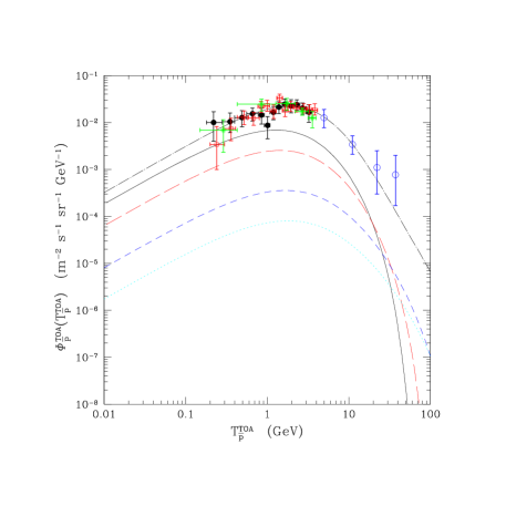
Figure 2: Primary TOA antiproton fluxes as a function of the antiproton kinetic energy. The dashed line denotes the secondary component, due to spallation of cosmic rays (i.e. the background) taken from Refs. PaperII ; revue . The other lines are representative fluxes from neutralino annihilation of different masses pb : the solid line refers to $m_{\chi}=60$ GeV, the long–dashed line to $m_{\chi}=100$ GeV, the short–dashed line to $m_{\chi}=300$ GeV and the dotted line to $m_{\chi}=500$ GeV. The astrophysical parameters for galactic propagation assume the best–fit values according to the analysis of Refs. PaperI ; pb . Solar modulation is calculated for a period of minimal solar activity. Full circles show the bess 1995–97 data bess95-97 ; the open squares show the bess 1998 data bess98 ; the stars show the ams data ams98 and the empty circles show the caprice data caprice .

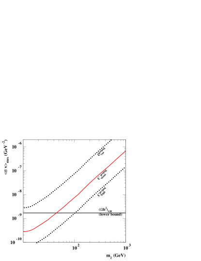
Figure 3: The solid line shows the maximum value (upper bound) of $\langle\sigma_{\textrm{ann}}v\rangle_{0}$ that can be allowed by the cosmic antiproton data in the fist energy–bin of BESS and AMS ($T^{\rm TOA}_{\rm p}=0.23$ GeV.) $\langle\sigma_{\textrm{ann}}v\rangle_{0}$ is the thermal average in the galactic halo of the WIMP annihilation cross section times relative velocity. The upper bound is shown as a function of the WIMP mass $m_{\chi}$ and has been derived using a median set of astrophysical parameters for the antiproton propagation. The upper and lower dotted lines show the uncertainty in the determination of the upper limit on $\langle\sigma_{\rm ann}v\rangle_{0}$ coming from the astrophysical uncertainties. The horizontal solid line shows the lower bound on $\langle\sigma_{\rm ann}v\rangle_{0}$ coming from the relic density of cold dark matter in standard cosmology, under the hypothesis that the WIMP annihilation cross–section in the early Universe $\langle\sigma_{\rm ann}v\rangle$ equals $\langle\sigma_{\rm ann}v\rangle_{0}$ (like in the case of $s$–wave dominance).

The antiproton component of cosmic rays has been measured by many detectors in space and the most recent results come from BESS, AMS and CAPRICE experiments. The standard production of cosmic antiprotons from spallation of nuclei on the diffuse Milky–Way gas is enough to explain the data PaperII ; revue , but the error–bars leave a small room also for an exotic antiproton signal. Such a signal could come from the annihilation of WIMPs in the Galaxy (see e.g. Ref. pb ). This situation is shown in Fig. 2, where the experimental data are plotted together with the background component and some examples of a signal coming from WIMP annihilation, as calculated in Ref. pb .

The antiproton flux produced in a point of cylindrical coordinates $(r,z)$ in the galactic halo, where the dark matter density is $\rho(r,z)$, depends on the annihilation cross section of the WIMPs averaged over their velocity distribution in the galactic halo $\langle\sigma_{\rm ann}v\rangle_{0}$ and on the final–state branching–ratios into the different possible final sates $F$ pb :

$$q_{\bar{p}}(r,z:T_{\bar{p}})=\langle\sigma_{\rm ann}v\rangle_{0}\frac{\rho^{2}(r,z)}{2m_{\chi}^{2}}\,\sum_{F}{\rm BR}(\chi\chi\rightarrow F)\,\left(\frac{dN^{F}_{\bar{p}}}{dT_{\bar{p}}}\right)$$ (17)

where $T_{\bar{p}}$ is the antiproton kinetic energy. The antiprotons then propagate and diffuse in the galactic medium until they reach the Earth position in the Galaxy of coordinates $(R_{\odot},0)$:

$$q_{\bar{p}}(r,z:T_{\bar{p}})\,\longrightarrow\,\Phi_{\bar{p}}(R_{\odot},0:T_{\bar{p}})$$ (18)

The process of propagation has been discussed in details in Ref. pb , where it has been shown that, contrary to the case of the spallation antiprotons PaperI , a large uncertainty in the low–energy tail of the antiproton signal is present, due to the current uncertainties on the astrophysical parameters which describe the diffusion and propagation processes pb ; PaperI . This uncertainty is about one order of magnitude up or down around the best fit result pb , for antiproton kinetic energies below 1 GeV where a signal may be more promisingly approached for WIMPs in the tens–hundreds of GeV mass range, and without the need of boosted enhancements on the dark matter density pb ; boost . The additional solar modulation effect introduces another source of uncertainty which is expected to be less important than the one due to galactic diffusion. Also the uncertainty coming from the dark matter profile is not very relevant, since antiprotons which reach the Earth are produced relatively close in the Galaxy, due to diffusion, and therefore they do not strongly feel the quite uncertain galactic–center mass distribution. Differences in the galactic halo shape affect the antiproton signal at most 20% pb . For a thorough discussion of all these topics and of the calculation of the antiproton signal which we also use in the present analysis, we refer to Ref. pb .

The antiproton signal is a powerful tool for constraining WIMP dark matter, since the amount of antiprotons produced by typical WIMPs which can account for the dark matter abundance of Eq. (1) is at the level of the background and may even exceed it sizably pb ; pbarlim . The astrophysical uncertainties limit somehow the capabilities of this type of signal, but nevertheless combined limits in the astrophysical–particle physics parameter space may be set, especially for relatively light WIMPs. Ref. pbarlim showed how WIMPs in the mass range from few GeV to hundreds of GeV are currently constrained by antiprotons searches. The possibility to set bounds mainly relies on the fact that the low–energy tail of the predicted antiproton signal may exceed the room left in the experimental uncertainty of the data over the calculated background. We make use of the same argument in the present discussion to use the antiproton signal to set limits on $\langle\sigma_{\rm ann}v\rangle_{0}$ and to transform these limits on bounds on the enhancement of the Hubble rate around WIMP freeze–out under the condition that the WIMPs satisfy the cosmological bound on the amount of cold dark matter.

A few comments are in order here before we proceed to discuss our strategy. First of all, we explain why we do not use also other indirect detection signals other than antiprotons. WIMP annihilation may obviously also produce gamma rays and positrons. However, contrary to the case of antiprotons which, almost independently of the halo density profile, are naturally at the level of the background and experimental data for cosmologically relevant WIMPs, both positrons and gamma rays usually require sizeable boosts in the dark matter density in order to reach detectable levels. This introduces a strong model–dependent variable which does not allow us to use these indirect signals as reliable tools for setting limits. For instance, a limit obtained from gamma–rays would fade out completely unless a very steep density profile is present at the galactic center. The same occurs for positrons, which need strongly clumped structures very close to our position in the Galaxy. Even though these indirect signals are very appealing for dark matter studies, they do not prove to be useful in the analysis we want to carry on in this paper. Very promising will potentially be antideuterons dbar , but for that we have to wait for the foreseen experimental set–ups able to access the required sensitivities gaps ; ams .

For similar reasons, we are concentrating our analysis on the low–energy tail of the antiproton flux: also at energies in the tens of GeV range (where CAPRICE data are available) a signal could manifest itself above the background, which is here fast decaying. Moreover, astrophysical uncertainties are less relevant at these energies. However, in order to have large signals in this range of energies, we need a suitable WIMP number density, which can be likely obtained only with some degree of over–density (due to the fact that we need here heavier WIMPs, whose number density is damped by the $m^{-2}$ factor) pb ; sweden . Again, since we do not want to add additional arbitrary inputs in our analysis (the boost factor), we focus on the low–energy tail.

Finally, we must remind that the antiproton signal depends on (and therefore can be constrained to set bounds on) $\langle\sigma_{\rm ann}v\rangle_{0}$, while the relic abundance depends on $\langle\sigma_{\rm ann}v\rangle$, i.e. on the thermal average on the annihilation cross section at a different (larger) temperature. A constraint on $\langle\sigma_{\rm ann}v\rangle_{0}$ is not therefore directly transferable to a bound on the WIMP relic abundance, and vice–versa. The usual expansion of the thermal average:

$$\langle\sigma_{\textrm{ann}}v\rangle=a+\frac{b}{x}+\cdot\cdot\cdot$$ (19)

holds in most of the cases, noticeable differences are when co–annihilation effects are present coannihil ; pole1 or when annihilation occurs close to a resonance or a threshold pole2 . However, in most of the typical cases, the thermal average of the annihilation cross section is mildly temperature–dependent. We will first discuss through the paper the case of temperature–independence, i.e.: $\langle\sigma_{\rm ann}v\rangle=\langle\sigma_{\rm ann}v\rangle_{0}=a$. We will then discuss how our results are changed when the first–order expansion of Eq. (19) is relevant. The most important effect on our results basically comes from the difference between the freeze–out and current value of $\langle\sigma_{\rm ann}v\rangle$, i.e. on the ratio:

$${\cal R}=\frac{\langle\sigma_{\rm ann}v\rangle_{T_{\rm f}}}{\langle\sigma_{\rm ann}v\rangle_{0}}$$ (20)

Therefore, an estimate of how our results would change, for instance when the relic abundance is determined by co–annihilation effects, is to assume a given value for ${\cal R}$ in relating $\langle\sigma_{\rm ann}v\rangle$ at freeze–out and $\langle\sigma_{\rm ann}v\rangle_{0}$. We also need to comment that, in order to apply the antiproton bound, the WIMP annihilation must proceed sizably to non-leptonic final states. In fact, for annihilation into leptons, antiprotons are not produced and our bounds are loosened by a factor given by the branching ratio into non-leptonic final states.

Let us now determine the upper limit on the WIMP annihilation cross section derived from the observational upper limit on the exotic cosmic antiproton flux. We do not attempt here a statistical analysis of the data as was done in Ref. pbarlim . We instead use a simpler approach which uses the most relevant information coming from the antiproton data and at the same time allows us to have an insight on the results, which could instead be more difficult to obtain by a statistical treatment of the data. This approach was the one also adopted in Ref. pb . We consider the experimental result in the lowest–energy bin at $T_{\bar{p}}^{\textrm{TOA}}=0.23$ GeV. By subtracting the background PaperII , we are left with a 90% C.L. upper limit for the exotic antiproton component at the top of the atmosphere (TOA) of: $\Phi_{\bar{p}}^{{\textrm{TOA}}}=2\cdot 10^{-3}\textrm{m}^{-2}\textrm{s}^{-1}\textrm{sr}^{-1}\textrm{GeV}^{-1}$ pb . In order to find the corresponding upper bound on the WIMP annihilation cross section we must specify our assumptions in the calculation of Eq. (17,18) of the expected antiproton flux for any given mass $m_{\chi}$ and cross section $\langle\sigma_{\rm ann}v\rangle_{0}$.

We assume an isothermal halo model with core radius 3.5 kpc and local dark matter density 0.3 GeV $\textrm{cm}^{-3}$. When nothing else is mentioned we use the mean values for the set of astrophysical parameters of the propagation and diffusion models given in Ref.pb , but we discuss also the set of parameters which provide the maximal and minimal antiproton flux, in order to properly take into account this intrinsic and dominant source of uncertainty. As for the antiproton spectrum, we assume for definiteness that the WIMP annihilate only into a $\bar{b}b$ pair, and we therefore use the corresponding spectra given in Ref. pb . A more generic annihilation final state would only mildly change our results (except for the already–mentioned leptonic final state).

The result on the upper bound on $\langle\sigma_{\rm ann}v\rangle_{0}$ is shown in Fig. 3 as a function of the WIMP mass and for the median, as well as maximal and minimal set of astrophysical parameters. We notice that the astrophysical uncertainty is severe, but nevertheless allows us to set limits on the maximal amount of $\langle\sigma_{\rm ann}v\rangle_{0}$ which is allowed in order not to go in conflict with the experimental data. The horizontal solid line instead shows the lower limit on $\langle\sigma_{\rm ann}v\rangle$ coming from the cosmological bound on the WIMP relic abundance of Eq. (1), in the case of temperature independent thermal average and standard cosmology. The figure clearly shows that there is tension between the cosmological bound and the antiproton limit: in the case of the median bound from antiproton, we see that WIMPs lighter than about 50–60 GeV lead to an antiproton signal which is in excess of the experimental bound. This tension is released if we consider the minimal set of astrophysical parameters (upper dotted curve), but the figure clearly shows that antiprotons are a powerful tool for setting limits. Ref. pbarlim already discussed in details this tensions and the corresponding limits. We instead here use this argument to set bounds on cosmological models: since the cosmological models we are discussing predict larger lower–bounds on $\langle\sigma_{\rm ann}v\rangle$, we see that the tension with antiproton data is enhanced and limits can be set on the maximal amount of enhancement of the Hubble rate at the time of WIMP freeze–out.

VI Constraining the Hubble rate with Dark Matter

In this Section we show how the combined constraints on the WIMP relic density and antiproton signal can strongly constrain the Hubble rate in the early Universe. Let us first recall our assumptions about the Hubble rate and the WIMPs. We assume that the Hubble rate is enhanced by a temperature–dependent factor $A(T)$ in the early Universe, for which we consider the parametrization of Eq. (5). At the temperature $T_{\textrm{f}}$ at which the WIMP would freeze out in the standard case, the enhancement factor is equal to the parameter $\eta$, $A(T_{\textrm{f}})=\eta$ (for $\eta\gg 1$). The slope of $A(T)$ is set by the parameter $\nu$. At a temperature $T=T_{\textrm{re}}$, the expansion rate ”re–enters” the standard one. We consider a general WIMP model characterized solely by a mass, $m_{\chi}$, and an annihilation cross section. We assume first that $\langle\sigma_{\textrm{ann}}v\rangle=\langle\sigma_{\rm ann}v\rangle_{0}$ is temperature independent, and therefore it determines both the relic abundance and the antiproton signal directly. The WIMP should explain the observational amount of cold dark matter of Eq. (1), i.e. it must be the dominant CDM component.

In the following we combine the relic density and antiproton constraints on the WIMP to obtain the upper bound on the enhancement of the Hubble rate. As we have discussed, this is possible because the Hubble rate together with the WIMP mass and cross section determines the WIMP abundance, and at the same time the WIMP cross section is bounded from above by the cosmic antiproton data. In Section VI.1 we find the mass dependent upper bound on $\eta$, i.e. the enhancement factor at the time of the WIMP freeze out. In Section VI.2 we determine the corresponding upper bound on the enhancement of the relic WIMP density as compared to standard cosmology. Finally, in Section VI.3 we analyze what happens to the bound on $\eta$ when some of our assumptions about the Hubble rate and the WIMP model are changed.

VI.1 Constraining the expansion rate

Let us in this section show our numerical results on the Hubble rate constraints derived from the relic density and antiproton bound. Our parametrization of the Hubble enhancement function Eq. (5) has three free parameters: $\eta$, $\nu$ and $T_{\textrm{re}}$ (while $T_{\textrm{f}}$ is set by the WIMP mass and cross section through Eq. (14)). As we shall see at the end of this section, the enhancement is basically independent of $T_{\textrm{re}}$, as long as $T_{\textrm{re}}\ll T_{\rm f}$. This can be understood also by means of the analytical approximations given in Appendix A. We choose to set $T_{\textrm{re}}=10^{-3}$ GeV throughout the paper as a reference value. This corresponds to the lowest value which can be safely assumed to be compatible with big bang nucleosynthesis scalartensorrelic . The enhancement of the Hubble rate is then studied in the two-dimensional parameter space $(\eta,\nu)$.

Let us now construct an exclusion plot in the $(\eta,\nu)$ plane. We first fix the WIMP mass at $m_{\chi}=500$ GeV as a reference value. Then, for each point in the $(\eta,\nu)$ plane we make a scan in the WIMP annihilation cross section $\langle\sigma_{\textrm{ann}}v\rangle$. The cross section together with the mass fixes $T_{\textrm{f}}$, which is the temperature at which the WIMP would freeze out in the standard cosmology scenario. We then solve the Boltzmann equation with the enhanced Hubble rate. We can now apply the first bound, namely the constraint Eq. (1) on the relic dark matter density. This constraint selects a small interval in $\langle\sigma_{\textrm{ann}}v\rangle$ for each $(\eta,\nu)$. Finally we apply the constraint coming from the cosmic antiproton data on $\langle\sigma_{\rm ann}v\rangle_{0}$, by means of the result shown in Fig.3, which gives us the upper bound on the annihilation cross section for any given mass.

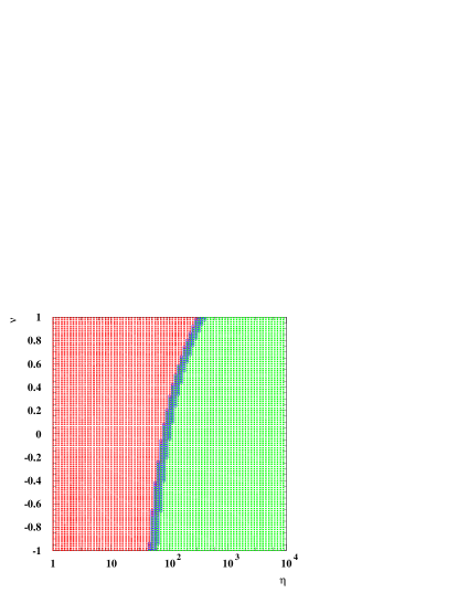
Figure 4: Exclusion plot in the $(\eta,\nu)$ plane for a WIMP mass of $m_{\chi}=500$ GeV. $\eta$ and $\nu$ are two of the parameters of the Hubble enhancement function. $\eta$ is the enhancement factor at the freeze–out temperature of the WIMP. The “re–entering” temperature has been fixed at $T_{\textrm{re}}=10^{-3}$ GeV. The WIMP annihilation cross section $\langle\sigma_{\rm ann}v\rangle$ is chosen for each point in order to fulfill the relic density constraint. This cross section has then been compared to the antiproton upper bound on the cross section. The central almost vertical band denotes points which have exactly the limiting value of the cross section; the points on the left of the band refer to cross sections below the antiproton upper bound; the points on the right of the band refer to cross section in excess of the antiproton upper bound.

In fig. 4 we show the exclusion plot in the $(\eta,\nu)$ plane. The points in the central almost–vertical band refer to annihilation cross sections $\langle\sigma_{\textrm{ann}}v\rangle$ equal to the maximum value allowed by the antiproton data (using the median set of astrophysical parameters) as shown in Fig. 3. The points on the left of the vertical band all refer to smaller values of the cross section and thus satisfy the antiproton bound. On the contrary, the points on the right are in disagreement with the antiproton data as they require a high cross section in order to fulfill the density constraint. Notice that the cross section is not uniquely determined by the density constraint, since for fixed values of $\eta$, $\nu$ and $m_{\chi}$ we can slightly vary the annihilation cross section to move around in the allowed density interval of Eq. (1). Similarly, points next to each other can have identical cross section and fulfill the density constraints with just slightly different values of the relic abundance . Thus, the width of the vertical band, that marks the antiproton bound, is due to the allowed interval of the relic abundance. Also, in the vertical band we do not only have models with a cross section equal to the antiproton limit, but also models with a slightly lower or higher cross section.

From fig. 4 we conclude that the constraint coming from the cosmic antiprotons produced by dark matter annihilation can be used to put constraints on the Hubble rate in the very early Universe. The figure shows that, for $m_{\chi}=500$ GeV, we get an upper bound on the enhancement factor $\eta$ of the Hubble rate at the WIMP freeze–out of around $10^{2}$ (with some dependence on the actual values of the slope parameter $\nu$). This bound on $\eta$ may be considered as significant: in Ref. scalartensorrelic we found perfectly viable scalar–tensor models with enhancement factors of up to $10^{4}$ at the WIMP freeze–out temperature, once the BBN, CMB and gravitational probe limits were satisfied. Our results shows that alternative, and even stronger, bounds on dark energy models can therefore be obtained also by looking at the imprints left on the dark matter properties by these modified cosmologies at the time dark matter formed in the early Universe, if we assume that dark matter is provided by a thermal relic.

Figure 5: The same as Fig. 4 but including the result for different WIMP masses. Going from left to right the vertical bands correspond to the antiproton bound for WIMP masses of 60 GeV, 100 GeV, 200 GeV, 400 GeV, 600 GeV and 1000 GeV respectively. For any given mass, the vertical band marks the limit between the excluded part of the parameter space to the right and the part to the left which is in agreement with the antiproton data. The “re–entering” temperature is $T_{\textrm{re}}=10^{-3}$ GeV.

The results in fig. 4 were calculated for a fixed WIMP mass of 500 GeV. Let us now explore how the bound on $\eta$ depends on the WIMP mass. The result is shown in fig. 5. Each vertical band corresponds to the maximum allowed cross section for any given mass according to fig. 3. Going from left to right in fig. 5, the vertical bands corresponds to the masses 60 GeV, 100 GeV, 200 GeV, 400 GeV, 600 GeV and 1000 GeV respectively. For any given mass, the part of the $(\eta,\nu)$ plane to the right of the vertical band is excluded by the antiproton data while the part to the left is allowed. The constraint on $\eta$ is very strong, especially for low WIMP masses. In particular, the figure shows that WIMPs lighter than about 60 GeV are close to being excluded. A word of caution is in order here: to make a precise claim on a lower bound on the WIMP mass would require a more thorough analysis, since we should include the uncertainty on the propagation and diffusion parameters for the calculation of the antiproton flux and also apply a more refined statistical analysis on the antiproton data. We will show the effect coming from the astrophysical parameters in Sect. VI.3, and we anticipate that for the less stringent set of parameters, WIMPs lighter than 60 GeV are perfectly viable. These results are in agreement with what is found in Ref. pbarlim where a careful analysis of the bounds that can be set to the WIMP parameters by antiproton data in standard cosmology has been performed.

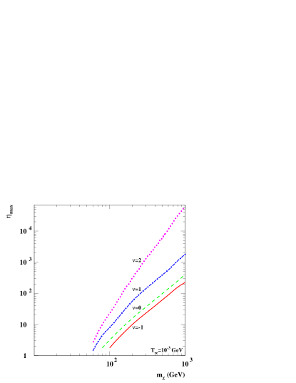
Figure 6: Upper limit on the value of $\eta$ obtained by imposing the combined constraints on the WIMP relic abundance and the WIMP antiproton signal. $\eta$ is the Hubble enhancement factor at the time where the WIMP freezes out in standard cosmology. The bound on $\eta$ is shown as a function of the WIMP mass for the slope parameter of the enhancement function $\nu=-1,0,1,2$. The parameter $T_{\textrm{re}}$ has been set to $10^{-3}$ GeV. $T_{\textrm{f}}$ is determined by the WIMP mass and cross section by means of the freeze–out condition of Eq. (14). The WIMP cross section is fixed at the limit of Fig. 3.

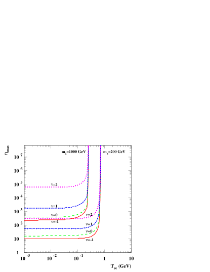
Figure 7: Upper bound on the Hubble enhancement parameter $\eta$ as a function of $T_{\textrm{re}}$, i.e. the temperature at which the Hubble expansion “re–enters” the standard evolution. The upper bound on $\eta$ is derived from the combination of the constraint on the WIMP relic density and antiproton signal. The numerical derivation is done for two different WIMP masses and four different values of the parameter $\nu$. The masses are $m_{\chi}=200$ GeV and $m_{\chi}=1$ TeV corresponding to $T_{\textrm{f}}\sim 7.46$ GeV respectively $T_{\textrm{f}}\sim 31.86$ GeV for the limiting cross section. The upper set of curves is for the high mass. For each of the two set of curves we have $\nu=2,1,0,-1$ when going from the top to the bottom.

From fig. 5 we see that the upper bound on $\eta$ increases less than an order of magnitude when the parameter $\nu$ is varied from $-1$ to $+1$ for any given mass. For large masses, the increase can be two orders of magnitude when we continue to $\nu=2$. This can be seen in fig. 6, which displays the mass dependence of the upper bound on $\eta$, as derived for four different values of $\nu$.

The behaviour of the upper bound on $\eta$ can be understood also by means of the analytic approximations of Appendix A. The conditions we want to satisfy at the same time are the following:

$$\Omega h^{2} \leq (\Omega h^{2})_{CDM}\quad\,\mbox{cosmological bound}$$ (21)

$$\langle\sigma_{\rm ann}v\rangle_{0} \leq \langle\sigma_{\rm ann}v\rangle_{0}^{\bar{p}}\quad\quad\,\mbox{antiproton bound}$$ (22)

where $(\Omega h^{2})_{CDM}$ is the maximal allowed value of the relic abundance constraint of Eq. (1) and $\langle\sigma_{\rm ann}v\rangle_{0}^{\bar{p}}$ is the upper limit on the annihilation cross section coming from Fig. 3. This limit may be approximated as: $\langle\sigma_{\rm ann}v\rangle_{0}^{\bar{p}}\simeq 0.95\cdot 10^{-12}\,m^{1.95}_{\chi}$ GeV^-2 for $m_{\chi}\mathrel{\mathop{\kern 0.0pt\hbox to0.0pt{\raise 0.86108pt\hbox{$>$}\hss}}\lower 3.87495pt\hbox{\kern-1.90002pt$\sim$}}60$ GeV. The two bounds transform in the following condition:

$$f(\eta)\leq\langle\sigma_{\rm ann}v\rangle_{0}^{\bar{p}}\,(\Omega h^{2})_{CDM}$$ (23)

where, by means of the approximations given in Appendix A:

$$f(\eta)={\cal C}\left[{\cal I}(x_{\rm f},\hat{x},\eta,\nu)+r_{G}\,\frac{1}{\hat{x}}\right]^{-1}$$ (24)

and ${\cal C}=s_{0}\,\rho_{c}^{-1}\,B^{-1}\,{\cal G}^{-1}(x_{f})$. The maximal value of $\eta$ occurs when $\eta$ saturates the bound of Eq. (23). It is easy to show that:

$$\eta_{\rm max} = \left[\frac{\langle\sigma_{\rm ann}v\rangle_{0}^{\bar{p}}\,(\Omega h^{2})_{CDM}}{{\cal C}(\nu-1)\,x_{\rm f}}\right]^{\nu}\sim m^{1.95\cdot\nu}_{\chi}\,\mbox{for $\nu>1$}$$

$$\eta_{\rm max} = \left[\frac{\langle\sigma_{\rm ann}v\rangle_{0}^{\bar{p}}\,(\Omega h^{2})_{CDM}}{{\cal C}(1-\nu)\,x_{\rm f}}\right]\sim m^{1.95}_{\chi}\,\mbox{for $\nu<1$}$$ (25)

and a slightly more complicated expression for $\nu=1$ (kination case). These behaviours are confirmed by our numerical calculations, where we approximately find $\eta_{\rm max}\propto m_{\chi}^{2.1}$ for $\nu=-1,0,1$ (with a slight dependence on which masses are used for the calculation) and $\eta_{\rm max}\propto m_{\chi}^{3.5}$ for $\nu=2$.

We have shown in this Section that we can use the combined constraints on the WIMP relic density and antiproton production to put an upper limit on $\eta$, i.e. we can constrain the Hubble expansion at a very early time in the history of the Universe, as $\eta=A(T_{\textrm{f}})$. The exact temperature at which we constrain the expansion in our discussion, i.e. the standard freeze out temperature $T_{\textrm{f}}$, does however depend on the WIMP mass. Approximately, $x_{\textrm{f}}$ is always of the order of 25 ($x_{\textrm{f}}=m_{\chi}/T_{\textrm{f}}$). Some numerical examples are: $T_{\textrm{f}}(m_{\chi}=60\,\textrm{GeV})\simeq 2.6$ GeV, $T_{\textrm{f}}(m_{\chi}=200\,\textrm{GeV})\simeq 7.5$ GeV, $T_{\textrm{f}}(m_{\chi}=600\,\textrm{GeV})\simeq 20$ GeV and $T_{\textrm{f}}(m_{\chi}=1000\,\textrm{GeV})\simeq 32$ GeV, where we have used the upper antiproton bound for the value of the WIMP annihilation cross section.

Fig. 7 shows the upper bound on $\eta$ as a function of $T_{\textrm{re}}$ for two different values of the WIMP mass and four different values of the parameter $\nu$. Models that stay below the upper bound of $\eta$ would give WIMPs that either are under-abundant or produce less antiprotons than the maximally allowed flux. Fig. 7 shows that the upper bound on $\eta$ is independent of $T_{\textrm{re}}$ as long as the latter is much smaller than the freeze out temperature. When the “re–entering” temperature is around one or two order of magnitudes below the standard freeze out temperature, $\eta_{\rm max}$ starts to increase and then becomes practically unbounded from above. In other words, one can increase the Hubble rate arbitrarily if this is done for a short amount of time. We see from fig. 7 that the “re–entering” temperature at which $\eta$ starts to get unbounded is lower for the higher mass case despite the fact that the freeze out temperature is higher for $m_{\chi}=1000$ GeV than for $m_{\chi}=200$ GeV. This can be understood from the analytic solution of the modified Boltzmann equation. We compare the contribution from the integration from the modified freeze out until the “re–entering” temperature (i.e. the time where we still have enhanced expansion) with the contribution from the integration from the “re-entering” temperature untill today. The first contribution dominates when the “re–entering” temperature is very low. The analytic analysis shows that the two contributions becomes equal approximately when $(\hat{T}_{\textrm{f}}-T_{\textrm{re}})/T_{\textrm{re}}=\eta[h_{\textrm{eff}}(x_{\textrm{re}})\sqrt{g_{\textrm{eff}}(\hat{x}_{\textrm{f}})}]/[h_{\textrm{eff}}(\hat{x}_{\textrm{f}})\sqrt{g_{\textrm{eff}}(x_{\textrm{re}})}]$, where $\hat{T}_{\textrm{f}}$ is the freeze out temperature in the modified scenario and where we have set $\nu=0$ for definiteness. If $\eta$ stays constant then $\Omega{h^{2}}\rightarrow(\Omega{h^{2}})_{\textrm{std}}$ when $(\hat{T}_{\textrm{f}}-T_{\textrm{re}})$ shrinks to zero. Alternatively, to avoid the WIMP to become under–abundant we have to increase $\eta$ indefinitely. Since $\hat{T}$ grows approximately linearly with mass ($\hat{T}_{\textrm{f}}=m_{\chi}/{\hat{x}_{\textrm{f}}}$ and $\hat{x}_{\textrm{f}}$ depends logarithmically on the mass and the cross section) while the upper bound on $\eta$ (fig. 6) is approximately proportional to the mass squared, it follows that $\eta$ becomes unbounded at lower $T_{\textrm{re}}$ for $m_{\chi}=1000$ GeV compared to $m_{\chi}=200$ GeV.

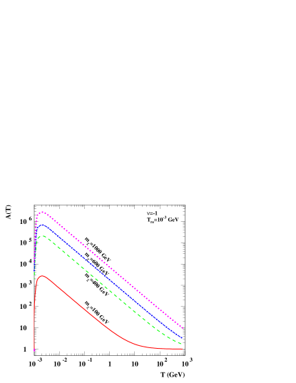
Figure 8: Maximum allowed values of the enhancement function $A(T)$ as a function of the temperature for our parametrization with $\nu=-1$ (close to a scalar–tensor cosmology). Notice that time is running from right to left. The limit is derived from $\eta_{\rm max}$. The solid red line refers to $m_{\chi}=100\ \textrm{GeV}$, the dashed green line to $m_{\chi}=400\ \textrm{GeV}$, the dash–dotted blue line to $m_{\chi}=600\ \textrm{GeV}$ and the dotted purple line to $m_{\chi}=1\ \textrm{TeV}$. For all the curves we use $T_{\textrm{re}}=10^{-3}$ GeV. The standard WIMP freeze–out temperature is given by the WIMP mass and the antiproton bound for the WIMP annihilation cross section.

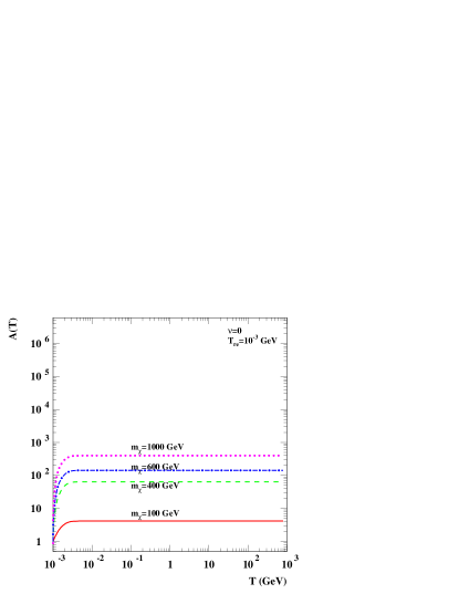
Figure 9: Same as Figure 8 but for $\nu=0$ (overall enhancement of Hubble rate, with standard temperature evolution).

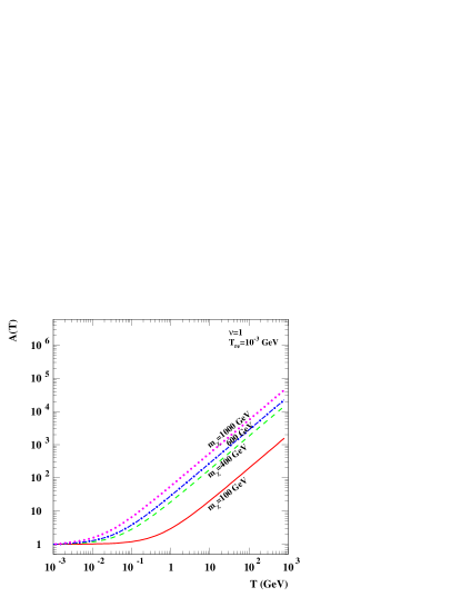
Figure 10: Same as figure 8 but for $\nu=1$ (kination case).

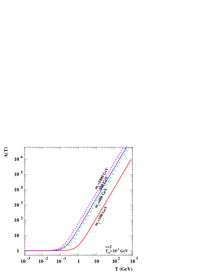
Figure 11: Same as figure 8 but for $\nu=2$ (RSII model Randall of extra–dimension cosmology)

The constraint on $\eta=A(T_{\textrm{f}})$ immediately constrains the Hubble enhancement function $A(T)$ given in Eq. (5) at any temperature once we know the WIMP mass and the cosmological model (i.e. the parameters $\nu$ and $T_{\textrm{re}}$). In Figs. 8, 9, 10 and 11 we show the maximum allowed enhancement function for different values of the WIMP mass and the $\nu$ parameter. The curves are derived for $T_{\textrm{re}}=10^{-3}\ \textrm{GeV}$. As we just saw, the upper bound on $\eta$ does not depend on $T_{\textrm{re}}$ when $T_{\textrm{re}}\ll T_{\textrm{f}}$. Thus, a change of the re-entering temperature would solely change the temperature at which $A(T)\rightarrow 1$. Figure 8, 9, 10 and 11 may be directly applied to constrain cosmological models with enhanced Hubble rate. For instance, for a scalar–tensor model like the one studied in Ref. scalartensorrelic , which refers to a situation close to $\nu=-1$ (the actual value was $\nu=-0.82$) and $T_{\rm re}=0.1$ GeV, by comparing Fig. 8 here and Fig. 6 of Ref. scalartensorrelic we can conclude that the model of Ref. scalartensorrelic is compatible with antiproton data only if the dark matter is composed by a WIMP with mass larger than 1 TeV. This example shows how constraining the antiproton data may be on otherwise viable dark energy models.

VI.2 The enhancement of the relic density

In this section we derive upper limits on the enhancement of the WIMP relic abundance in modified cosmologies as compared to the standard case, under the constraint that $\Omega h^{2}$ in the modified scenario satisfies the bound of Eq. (1). This constraint alone is not actually enough to constrain the enhancement of the density, as we shall see. When the antiproton bound for the WIMPs is applied we find an upper bound on the density enhancement which is practically independent of the parameter $\nu$, but that is of the same order of magnitude as the upper bound on $\eta$.

As in the previous section we start by making a study in the $(\eta,\nu)$ plane for a WIMP mass $m_{\chi}=500$ GeV. As for Fig. 4, we make a scan in $\langle\sigma_{\textrm{ann}}v\rangle$ for each $(\eta,\nu)$ and keep models where the WIMP density, as calculated with the enhanced Hubble rate, fulfills the density constraint. For each of these models we calculate also the WIMP density as it would be in the standard case and we then find the ratio $R=(\Omega{h}^{2})/(\Omega{h}^{2})_{\textrm{GR}}$.

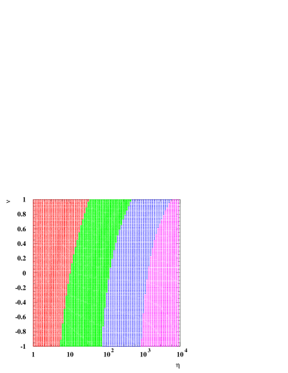
Figure 12: Contour plot of the enhancement $R=(\Omega{h}^{2})/(\Omega{h}^{2})_{\textrm{GR}}$ of the WIMP relic abundance in a scenario with enhanced Hubble rate compared to the standard GR cosmology. The different bands refer to (from left to right): $1\leq R\leq 10$, $10<R\leq 100$, $100<R\leq 1000$, $1000<R$. The highest value of $R$ is around $7.5\cdot{10}^{3}$. We have fixed $m_{\chi}=500$ GeV and $T_{\textrm{re}}=10^{-3}$ GeV. For all points, the WIMP relic–density, as calculated in the modified cosmology, satisfies the dark matter density constraint.

Fig. 12 shows contours of values of $R$. Going from low to high values of $\eta$, the different regions correspond to $1\leq R\leq 10$, $10<R\leq 100$, $100<R\leq 1000$, $1000<R$ with the highest value being around $7.5\cdot{10}^{3}$. If we had continued to higher values of $\eta$ we would have obtained even larger enhancements of the WIMP density. From the previous section we know that $\eta$ can be bounded from above by requiring that the WIMP fulfills the constraint coming from the cosmic antiproton data. For $m_{\chi}=500$ GeV the bound on $\eta$ was found in Fig. 4. When we compare this figure with the contours of $R$ in fig. 12, we conclude that the antiproton data leads to the upper limit $R\sim{100}$ for $m_{\chi}=500$ GeV. We also see that the shape of the contours of $R$ are very similar to the band in Fig. 4 which marks the limiting cross section. We therefore expect the upper bound on $R$ to be almost independent of $\nu$. The final thing to note is that the numerical value of the upper bound on $R$ and $\eta$ are of the same order of magnitude.

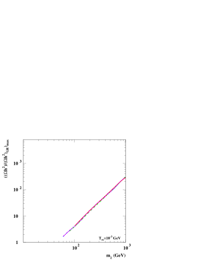
Figure 13: Upper limit of $R=(\Omega{h}^{2})/(\Omega{h}^{2})_{\textrm{GR}}$ as a function of the WIMP mass. The bound comes from the combination of the WIMP relic density constraint and the antiproton bound. The lines, which practically fall on top of each-other, refer to: $\nu=-1$, $\nu=0$, $\nu=1$ and $\nu=2$. The mass lower limit depend on $\nu$ (and it depends on the assumption of astrophysical parameters, which have been fixed to their median set in the figure). In the figure we have fixed $T_{\textrm{re}}=10^{-3}$ GeV.

The upper bound on the relic density enhancement $R$ as a function of the WIMP mass is shown in fig. 13, for the four representative values of the parameter $\nu$. The approximate behaviour $R\propto m_{\chi}^{1.9}$ can be understood by means of the analytical approximation we already discussed.

VI.3 Changing the assumptions

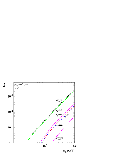
Figure 14: Upper bound on $\eta$ as a function of the WIMP mass under different assumptions, as derived from the combined constraint on the WIMP relic abundance and antiproton flux. All curves have $T_{\textrm{re}}=10^{-3}$ GeV and $\nu=-1$. The reference case is the red solid curve which is identical to our previous result in Fig. 6. The uppermost and lowermost dotted lines delimit the band due to the uncertainty on the astrophysical parameters for the antiproton propagation and diffusion. The uppermost curve is for the minimal set of astrophysical parameters while the lowermost is for the maximal set of parameters. The two dash–dotted lines, instead, include a $p$-wave contribution for the annihilation in the early Universe. For the upper green curve the $p$-wave factor is $r_{p}=10$ (see text) and for the lower purple curve we have $r_{p}=0.5$. The dotted line which falls on top of the red solid (mean) line is calculated with the Hubble enhancement function $A_{2}(T)$ with a change in the post-freeze–out temperature behaviour given by the parameter $\alpha=100$.

In this Section we show how the upper bound on the Hubble enhancement $\eta$ moves when some of our assumptions are changed. We are going to consider three kinds of modifications: we shall consider a temperature–dependent annihilation thermal cross section, by adding a $p$-wave contribution; we change the parametrization of the Hubble enhancement $A(T)$; finally we take into account the uncertainty of the propagation and diffusion of the cosmic antiproton signal.

Let us first consider what happens if our assumption about pure $s$-wave annihilation does not hold. In this case $\langle\sigma_{\rm ann}v\rangle$, relevant for the relic abundance, and $\langle\sigma_{\rm ann}v\rangle_{0}$, relevant for the antiproton calculation, are no longer equal. By adding a $p$-wave term $b/x$ in the temperature expansion of Eq. (19), $\langle\sigma_{\textrm{ann}}v\rangle$ turns out to be larger (or smaller, depending on the sign of $b$) in the early Universe than it is today where the $p$-wave contribution is negligible. The ensuing limit we obtain is less (more) stringent than the one we would obtain for pure $s$–wave annihilation, depending whether $b$ is positive or negative. Fig. 14 shows the effect for two representative cases in terms of $r_{p}=b/(a\,x_{\rm f})$: $r_{p}=0.5$ (lower dash–dotted purple line) and $r_{p}=10$ (upper dash–dotted green line). The last value is actually extreme and it has been considered to make an example.

We notice that the results we obtain for a non negligible $p$–wave case are similar to what we would obtain by assuming a value for the ratio ${\cal R}$ in Eq. (20) of the order of ${\cal R}=(1+\omega\,r_{p})$, where $\omega\sim{\cal O}(1)$ depends on details of the integrals given in Eq. (16), and therefore also on the cosmological model (simple analytical expressions may be derived by means of the approximations of Appendix A). The cases shown in Fig. 14 refer to ${\cal R}\simeq 1.2-1.5$ for $r_{p}=0.5$ and ${\cal R}\simeq 6-10$ for $r_{p}=10$. The figure therefore shows that the bound on $\eta_{\rm max}$ is sensitive to large values of the ratio ${\cal R}$, as expected. In the case, for instance, of coannihilations, for which ${\cal R}$ may be a large number (even some orders of magnitude) we see that the bounds from antiprotons are much less stringent. Approximately, the change in the upper bound on $\eta$ obtained in Eqs. (25) for the case of time–independent cross section, can now be rephrased as:

$$\eta_{\rm max} = \left[\frac{{\cal R}\,\langle\sigma_{\rm ann}v\rangle_{0}^{\bar{p}}\,(\Omega h^{2})_{CDM}}{{\cal C}(\nu-1)\,x_{\rm f}}\right]^{\nu}\quad\mbox{for $\nu>1$}$$

$$\eta_{\rm max} = \left[\frac{{\cal R}\,\langle\sigma_{\rm ann}v\rangle_{0}^{\bar{p}}\,(\Omega h^{2})_{CDM}}{{\cal C}(1-\nu)\,x_{\rm f}}\right]\quad\ \ \mbox{for $\nu<1$}$$

with, again, a slightly more complicated expression for $\nu=1$.

Now, let us go back to the situation where we have only a temperature–independent thermal cross section but instead we modify the enhancement of the Hubble rate. Let us assume, instead of the enhancement $A(T)$ defined in Eq. (5), the following function:

$$A_{2}(T)=1+\eta\,\left(\frac{T}{T_{\textrm{f}}}\right)^{\nu}\,\tanh^{2}\left(\frac{T-T_{\textrm{re}}}{\alpha T_{\textrm{re}}}\right)$$ (26)

The difference between $A(T)$ and $A_{2}(T)$ is that in the latter case the tanh is squared and in its argument we have introduced a factor $\alpha$. This modification aims at obtaining (for large values of $\alpha$) a “re–entering” into the standard regime less steep than in the previous case. This is illustrated in fig. 15.

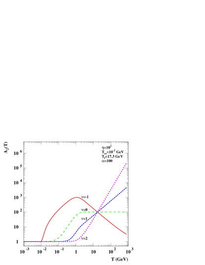
Figure 15: Enhancement function $A_{2}(T)$ of Eq. (26) as a function of the temperature. Notice that time runs from right to left. The solid red line has $\nu=-1$, the dashed green line $\nu=0$, the dash-dotted blue $\nu=1$ and the dotted purple line has $\nu=2$. We have chosen $\alpha=100$. All other parameters are identical to those of $A(T)$ in Fig. 1, i.e. $\eta=10^{2}$, $T_{\textrm{re}}=10^{-2}$ GeV and $T_{\textrm{f}}=17.3$ GeV.

A comparison between the upper bound on $\eta$ in the case of a Hubble enhancement $A(T)$ and $A_{2}(T)$ is shown again in Fig. 14. The central blue dotted line is for $A_{2}(T)$ with $\alpha=100$, $T_{\textrm{re}}=10^{-3}$ and $\nu=-1$. It can be seen that this line practically falls on top of the limit (red solid line) derived for $A(T)$ (and $T_{\textrm{re}}=10^{-3}$, $\nu=-1$). This result shows that the actual shape of the enhancement function around “re–entering” is not of major importance as long as the “re–entering” occurs long after the WIMP freeze out.

Let us finally consider how the upper bound on $\eta$ is affected by the uncertainty in the astrophysical parameters of the propagation and diffusion of the antiproton flux. We refer for this uncertainty to Ref. pb . Up to now, we have used a set of astrophysical parameters which provides the median value of the antiproton flux pb . This set of parameters is the one which best fits cosmic ray observations, mainly the B/C ratio PaperII . We now show in Fig. 14 the results obtained for the allowed range of astrophysical parameters, which give a maximal and minimal antiproton flux. The uppermost dotted curve in Fig. 14 shows the result obtained using the “minimal” set of astrophysical parameters for the propagation and diffusion, while the lowermost dotted curve shows the result as calculated using the “maximal” set. These curves should be compared to the central solid curve, which is our previous result obtained with the best–fit parameters. For all the curves we have $T_{\textrm{re}}=10^{-3}$ GeV and $\nu=-1$. We see that the uncertainty in the propagation function causes an uncertainty of almost one order of magnitude in both direction for the upper limit of $\eta$, as expected from the discussion in Sec. V and from the analytical approximations of Eq. (25).

From Fig. 14 we also see that a different choice on the astrophysical parameters may lead to a different lower limit on the WIMP mass, as a consequence of the fact that lowering the bound on the cross section (for the maximal set of astrophysical parameters) causes the upper bound on $\eta$ to decrease. This can be seen from the plot of the $(\eta,\nu)$ plane in Fig. 5. For a selection of masses this shows the bound as calculated with the median propagation function. For a given mass, the region to the left (i.e. at smaller $\eta$) is allowed by the antiproton data as the cross section here is lower. Thus, when we decrease the upper bound on the cross section, i.e. increase the effect of the propagation parameters, all the bounds in Fig. 5 will move to smaller $\eta$ (in particular the lower masses will move outside the plot). This is consistent with the results of Ref. pbarlim .

VII Antiproton flux constraints on some specific models

As we discussed in the previous sections, the maximum allowed antiproton flux gives interesting model–independent constraints on the maximum allowed enhancement of the expansion rate at dark matter freeze out. Let us now discuss these constraints in connection to the specific cosmological models we shortly introduced in Section III.

VII.1 Scalar-tensor theories

As mentioned in section III.1, we do not have a general analytical correspondence between the Hubble expansion rate in the scalar–tensor model and our parametrization (5). However, the numeric example of reference scalartensorrelic , which assumes a slowly varying scalar field, can be described by our parametrization with $\nu=-0.82$ and $\eta=A(\varphi(T_{\textrm{f}}))$, where $A(\varphi)$ is the Weyl factor, which in this case gives the Hubble enhancement function $A(T)$. From figure 6 we get the upper bound:

$$A\left(\varphi(T_{\textrm{f}})\right)<\mathcal{O}(10^{2})\qquad\textrm{for}\quad m_{\chi}\leq\mathcal{O}(500\textrm{GeV})$$ (27)

and $T_{\textrm{f}}=\mathcal{O}(10\textrm{GeV})$. From figure 8 we can also find the upper bound on $A(T)=A(\varphi)$ at earlier times. We see that $A(\varphi)<10$ for $T>\mathcal{O}(10^{2}\textrm{GeV})$ and $m_{\chi}\leq\mathcal{O}(500\textrm{GeV})$. It is interesting to observe that our results strongly constrain Fig. 5 of scalartensorrelic in which it could seem that properly choosing the initial conditions for the scalar field, each enhancement for the expansion rate is allowed. Antiproton data limit this possibility.

VII.2 Kination

In sec. III.2 we found that $\nu=1$ and $\eta=\sqrt{\eta_{\Phi}}=\sqrt{\rho_{\Phi}\left(T_{\textrm{f}}\right)/\rho_{r}\left(T_{\textrm{f}}\right)}$ can be used to describe the enhanced expansion rate during a kination phase.

We know from Sec. VI.2 that $\eta$ is approximately equal to the WIMP density enhancement. This is in agreement with the conclusions of the earlier references on kination and enhanced WIMP density; see e.g. Ref. Salati and Ref. profumoullio . In Ref. profumoullio they found that the maximal density enhancement compatible with the BBN bounds is of the order of $10^{6}$ (for WIMP masses smaller than 1 TeV), i.e. $\eta_{\Phi}<10^{12}$. With our argument based on the maximum allowed antiproton flux we can derive a much stronger constraint on this scenario. The most conservative bound is found for large masses. For $m_{\chi}<1\textrm{TeV}$ (and $\nu=1$) we have $\eta<\mathcal{O}(10^{3})$ and so $\eta_{\Phi}<10^{6}$. While for light WIMPs ($m_{\chi}<\mathcal{O}(10^{2}\textrm{GeV})$) we have the much more stringent bound $\eta<10$ and so $\eta_{\Phi}<10^{2}$.

VII.3 Extra Dimensions

As mentioned in section III.3, the RSII model Randall gives rise to an enhanced expansion rate which can be described by our parametrization with the values of the parameters $\nu=2$ and $\eta=\sqrt{\rho_{r}\left(T_{\textrm{f}}\right)/(2\lambda)}$. Where $\lambda$ is the tension on the brane and $\rho_{r}$ is the radiation energy density. The upper bound on $\eta$ therefore gives us a lower bound on the brane tension. The upper bound on $\eta$ for $\nu=2$ is shown in Fig. 6. For $\eta<\mathcal{O}(10^{2})$, which is true for WIMP masses $m_{\chi}<\mathcal{O}(10^{2}\textrm{GeV})$, we get the most stringent bound. With $T_{\textrm{f}}\simeq 5\ \textrm{GeV}$ and $g_{\textrm{{eff}}}(T_{\textrm{f}})\simeq 9^{2}$ we find the bound $\lambda>\mathcal{O}(1\textrm{GeV}^{4})$. A more conservative bound is found for higher masses. For $m_{\chi}=\mathcal{O}(500\ \textrm{GeV})$ we have $\eta<\mathcal{O}(10^{4})$ and $T_{\textrm{f}}\simeq 20\ \textrm{GeV}$, leading to $\lambda>\mathcal{O}(10^{-2}\textrm{GeV}^{4})$. Finally, using the relation Durrer

$$\lambda=\frac{3}{4\pi}\frac{M_{5}^{6}}{M_{pl}^{2}}$$ (28)

where $M_{pl}$ is the four dimensional Plank mass and $M_{5}$ the five dimensional one, we can derive a lower bound on $M_{5}$. For the most stringent bound on $\lambda$ we get $M_{5}>3\cdot 10^{3}\ \textrm{TeV}$, while the more conservative bound just give a small change, $M_{5}>10^{3}\ \textrm{TeV}$. We observe that the BBN bound is $\lambda>1\ \textrm{MeV}^{4}$ and so $M_{5}>30\ \textrm{TeV}$, Durrer . Therefore in this context, our analysis based on the antiproton flux is much more stringent than the one coming form the BBN constraint.

VIII Conclusion

The expansion rate of the Universe in the era before BBN is predicted to be different from the one of standard FRW cosmology in a host of cosmological models which are derived either from modification of General Relativity, or from brane physics, or from attempts to provide a consistent explanation to dark energy. In the present paper we concentrated on models which predict an enhancement of the expansion rate, like e.g. those discussed in Ref. scalartensorrelic where the dark energy problem finds a solution in a scalar–tensor theory of gravity with an exponential run–away behaviour of a scalar field, in kination models like those of Ref. Salati ; Rosati ; profumoullio ; Pallis , in D–brane models like the RSII model of Ref. Randall or models of modified cosmology like those in Ref. Barrow ; kamionkowskiturner . These enhancements may be sizeable, without evading the post–BBN bounds (light primordial element production, CMB anisotropies, gravitational tests) which may be applied to these cosmological models: the enhancements may reach up to four scalartensorrelic or even six Salati ; profumoullio orders of magnitude. However, an imprint of this enhancement may be left on the properties of the particles responsible of the dark matter. This happens if the enhancement of the expansion rate occurs close to the time when the dark matter particles decouples from the thermal bath: this possibility relies on the fact that the cosmological bound on the amount of dark matter can be fulfilled by particles with larger annihilation cross section, as compared to standard cosmology scalartensorrelic ; Salati , due to an anticipated freeze–out. In this situations, indirect detection signals are typically enhanced, as long as the thermal cross section responsible of the relic abundance is close to the one which determines the indirect detection signals (like e.g. when the typical temperature expansion of the thermal cross section is applicable).

Cosmic antiprotons produced by WIMPs in the Galaxy are currently the best option for constraining particle dark matter annihilation cross sections pbarlim ; pb , since they are not strongly dependent on assumptions on the dark matter density profile, like instead is the case of the gamma–ray signal. Also, cosmic antiprotons produced by WIMPs are naturally predicted to be at the level of the background and of the data, when the WIMP accounts for the CDM content of the Universe, and without invoking high degrees of over–densities in the galactic neighbourhood pb . Since the experimental data are in good agreement with the expected background PaperII ; revue , not much room is left for an exotic component and therefore antiprotons may be used to set constraints pb ; pbarlim .

In this paper we exploited the effect induced on the antiproton signal by an increased expansion rate, to set bounds on the maximal enhancement of the expansion rate which can be allowed in the early Universe in a pre–BBN epoch note on reduction . These limits apply to an evolutionary phase close to dark matter decoupling (i.e. at temperatures of the Universe in the range of 1–30 GeV, for dark matter of about 10–1000 GeV mass) and are subject to the (quite reasonable) hypothesis that dark matter is a thermal relic. The bounds we have obtained are quite strong, especially for light dark matter. Our main result is summarized by Fig. 6. For WIMP masses lighter than 100 GeV, the bound on the Hubble–rate enhancement ranges from a factor of a few to a factor of 30, depending on the actual cosmological model, while for a mass of 500 GeV the bound falls in the range 50–500. These bounds are affected by the still large astrophysical uncertainties in the calculation of the antiproton signal pb , which reflects in a factor of 5 more stringent, or a factor of 10 more loose bounds. Nevertheless, the limits we obtain are much more stringent than the possible enhancement of these cosmological models.

A caveat is in order here: whenever the effective thermal annihilation cross section in the early Universe (responsible for the relic abundance) is sizably larger than the one in the galactic halo (which determines the antiproton signal) the bounds we determine are necessarily loosened. This occurs when coannihilation effects are relevant in determining the relic abundance. In this case the annihilation cross section in the Galaxy is typically much smaller than the effective one which sets the decoupling: in this case our limits still apply, but they are less constraining, approximately by the ratio of the two cross sections. We nevertheless notice that the occurrence of coannihilation is usually an accidental feature. Another case where our limits are less severe is when WIMP annihilation occurs mostly into leptons: in this case antiprotons are not produced and our bounds are loosened by a factor given by the branching ratio into non-leptonic final states. In all other situations, which represent the most typical cases, the limits we quote are actually necessarily present.

Finally, we applied our bounds to set constraints on some specific models. In the case of the scalar–tensor dark energy models of Ref. scalartensorrelic , we constrain the enhancement to be less than a factor 100 for dark matter lighter than 500 GeV. In the case of kination models, the maximal enhancement is 1000 for WIMPs lighter than 1 TeV, while for dark matter lighter than 100 GeV the enhancement must be below 10. Finally, for the Randall–Sundrum D–brane model of Ref. Randall , our limit may be used to set bounds on the tension on the brane: for WIMPs lighter than 100 GeV, the string tension must be larger than 1 GeV⁴; for heavier dark matter, the bound is 10^-2 GeV⁴. These limits reflect in a lower bound of about 10³ TeV on the 5–dimensional Planck mass and are much more severe than the usual constraints derived from BBN physics.

Appendix A Approximate Boltzmann–equation solutions for the modified Hubble rate

The Boltzmann equation Eq. (12) may be easily solved for a modified Hubble rate as defined in Eq. (5) by suitable approximations. We first make explicit the temperature (or $x=m_{\chi}/T$) dependence in Eq. (12) by rewriting the equation in the usual form:

$$\frac{dY}{dx}=-\sqrt{\frac{\pi}{45G}}\frac{h_{\textrm{eff}}(x)}{\sqrt{A^{2}(x)g_{\textrm{eff}}(x)}}\frac{m_{\chi}}{x^{2}}\langle\sigma_{\textrm{ann}}v\rangle(Y^{2}-Y^{2}_{\textrm{eq}})$$ (29)

where $G$ is the Newton constant. The standard cosmology case is recovered for $A(T)=1$.

We first define the temperature of particle freeze–out as the temperature $T_{f}$ when:

$$Y(x_{\rm f})=(1+c)Y_{\rm eq}(x_{\rm f})$$ (30)

with $c$ a constant of order 1 and $Y_{\rm eq}(x)=45\,\times\,2^{-5/2}\pi^{-7/2}\,g\,h^{-1}_{\rm eff}(x)\,x^{-3/2}\,\exp(-x)$ is the equilibrium abundance of a non–relativistic particle with internal degree of freedom $g$. Condition (30) and Eq. (29) lead to the following implicit expression for the freeze–out temperature:

$$x_{\textrm{f}}=\ln\left[\frac{2c}{1+c}0.038\,m_{\textrm{pl}}\,g\,m_{\chi}\frac{\langle\sigma_{\textrm{ann}}v\rangle_{x_{\textrm{f}}}}{x_{\textrm{f}}^{1/2}\,A(x_{\rm f})\,g^{1/2}_{\textrm{eff}}(x_{\textrm{f}})}\right]$$ (31)

where $m_{\rm pl}$ is the Planck mass. For definiteness, we use $c=1$ throughout the paper. The standard freeze–out temperature is obtained when $A(T)=1$ around the time of particle decoupling. The models we are considering, where $A(T)>1$ at that epoch, imply a smaller $x_{\rm f}$, i.e. a larger freeze–out temperature $T_{f}$.

The current value $Y_{0}$ of the comoving abundance is then obtained by integrating Eq. (29) from $x_{\rm f}$ down to $x_{0}\rightarrow\infty$, neglecting the WIMP production term:

$$\frac{dY}{dx}=-\sqrt{\frac{\pi}{45G}}\frac{h_{\textrm{eff}}(x)}{\sqrt{A^{2}(x)g_{\textrm{eff}}(x)}}\frac{m_{\chi}}{x^{2}}\langle\sigma_{\textrm{ann}}v\rangle Y^{2}$$ (32)

which gives the solution:

$$\frac{1}{Y_{0}}=\frac{1}{Y_{\rm eq}(x_{\rm f})}+B\,m_{\chi}\,\int_{x_{\rm f}}^{\infty}\frac{{\cal G}(x)\,\langle\sigma_{\textrm{ann}}v\rangle}{A(x)\,x^{2}}\,dx$$ (33)

where $B=(\pi/45G)^{1/2}$ and ${\cal G}(x)=h_{\textrm{eff}}(x)/\sqrt{g_{\textrm{eff}}(x)}$. The WIMP relic abundance is then obtained by means of Eq. (13).

For large enhancements of the Hubble rate around the WIMP freeze–out, i.e. for large values of the parameter $\eta$, we may approximate $A(T)$ as a power–law function with exponent $\nu$. If $\nu<0$, we may assume this behaviour all the way down to the re–entering temperature $x_{\rm re}$:

$$A(T)\simeq\eta\left(\frac{T}{T_{f}}\right)^{\nu}=(\eta\,x_{\rm f}^{\nu})\,x^{-\nu}$$ (34)

When $\nu>0$ the above approximation may not be used up to $x_{\rm re}$, because $A(x)$ approaches unity as the Universe cools down (see Fig. 1) and therefore we cannot neglect the 1 in Eq. (5). We define as $x_{1}$ the temperature when $(\eta\,x_{\rm f}^{\nu})\,x^{-\nu}\simeq 1$, i.e. $x_{1}=x_{\rm f}\eta^{1/\nu}$. In this case we approximate:

$$A(T)\simeq\left\{\begin{array}[]{ll}(\eta\,x_{\rm f}^{\nu})\,x^{-\nu}&\quad\quad\quad x\mathrel{\mathop{\kern 0.0pt\hbox to0.0pt{\raise 0.86108pt\hbox{$<$}\hss}}\lower 3.87495pt\hbox{\kern-1.90002pt$\sim$}}x_{1}\\ 1&\\ \end{array}\right.$$ (35)

Below $x_{\rm re}$, in any case $A(T)=1$ by definition.

With these approximations, the solution of Eq. (33) for a temperature–independent annihilation cross section $\langle\sigma_{\textrm{ann}}v\rangle=a$ is:

$$\frac{1}{Y_{0}} = \frac{1}{Y_{\rm eq}(x_{\rm f})}$$

$$+ B\,m_{\chi}\,a\,{\cal G}(x_{\rm f})\,\left[{\cal I}(x_{\rm f},\hat{x},\eta,\nu)+r_{G}\,\frac{1}{\hat{x}}\right]$$

where $\hat{x}=\min[x_{1},x_{\rm re}]$ and $r_{G}={\cal G}(\hat{x})/{\cal G}(x_{\rm f})$ is typically around 0.5–1 for WIMPs masses in the range GeV–TeV. For large enhancements ($\eta\gg 1$) and a low re–entering temperature, typically: $\hat{x}=x_{1}$ for $\nu>0$ and $\hat{x}=x_{\rm re}$ for $\nu<0$. In Eq. (A) we have assumed a slowly–varying ${\cal G}(x)$ in the integrals.

In our discussion in the text, typically the relevant term in Eq. (A) is the one which contains the function ${\cal I}(x_{\rm f},\hat{x},\eta,\nu)$: the other two terms may be usually neglected to a few percent level of approximation. This relevant function is easily found to be:

$${\cal I}=\frac{1}{\nu-1}\,\frac{1}{x_{\rm f}\,\eta^{1/\nu}}$$ (37)

for $\nu>1$, then

$${\cal I}=\frac{1}{1-\nu}\,\frac{1}{x_{\rm f}\,\eta}$$ (38)

for $\nu<1$ and finally

$${\cal I}=\frac{1}{x_{\rm f}}\,\frac{\ln(\eta)}{\eta}$$ (39)

for $\nu=1$ (kination).

- (1) D.N. Spergel et al. (WMAP Collaboration), [arXiv:astro–ph/0603449] (submitted to Astrophys. J.)
- (2) A reduction of the expansion rate is also possible; see e.g. Ref. reduction . We are not going to discuss these models here, since when the Hubble rate is rduced, the antiproton bounds derived in the paper does not lead to relevant constraints.
- (3) R. Catena, M. Pietroni and L. Scarabello, Phys. Rev. D 70, 103526 (2004) [arXiv:astro-ph/0407646]; C. de Rham, T. Shiromizu and A. J. Tolley, [arXiv:gr-qc/0604071].
- (4) R. Catena, N. Fornengo, A. Masiero, M. Pietroni and F. Rosati, Phys. Rev. D 70, 063519 (2004) [arXiv:astro-ph/0403614].
- (5) P. Salati, Phys. Lett. B 571, 121 (2003).
- (6) F. Rosati, Phys. Lett. B 570, 5 (2003) [arXiv:hep-ph/0309124].
- (7) S. Profumo and P. Ullio, JCAP 0311, 006 (2003) [arXiv:hep-ph/0309220]
- (8) C. Pallis, JCAP 0510, 015 (2005) [arXiv:hep-ph/0503080].
- (9) J. D. Barrow, Nucl. Phys. B 208, 501 (1982).
- (10) M. Kamionkowski and M. S. Turner, Phys. Rev. D 42, 3310 (1990).
- (11) L. Randall and R. Sundrum, Phys. Rev. Lett. 83, 4690 (1999).
- (12) F. Donato, N. Fornengo, D. Maurin, P. Salati and R. Taillet, Phys. Rev. D69, 063501 (2004) [arXiv:astro-ph/0306207].
- (13) A. Bottino, F. Donato, N. Fornengo and P. Salati, Phys. Rev. D72, 083518 (2005).
- (14) R. H. Cyburt, B. D. Fields, K. A. Olive and E. Skillman, Astropart. Phys. 23, 313 (2005) [arXiv:astro-ph/0408033].
- (15) Y. Wang and P. Mukherjee, [arXiv:astro-ph/0604051].
- (16) G. B. Zhao, J. Q. Xia, B. Feng and X. Zhang, [arXiv:astro-ph/0603621].
- (17) J. Albert et al. [SNAP Collaboration], [arXiv:astro-ph/0507460].
- (18) B. Bertotti, L. Iess and P. Tortora, Nature 425, 374 (2003).
- (19) T. Damour, [arXiv:gr-qc/9606079], lectures given at Les Houches 1992, SUSY05 and Corfu’ 1995.
- (20) G. Esposito-Farese and D. Polarski, Phys. Rev. D 63, 063504 (2001) [arXiv:gr-qc/0009034].
- (21) R. H. Dicke, Phys. Rev. 125, 2163 (1962).
- (22) R. Catena, M. Pietroni and L. Scarabello, [arXiv:astro-ph/0604492].
- (23) P. J. Steinhardt, L. M. Wang and I. Zlatev, Phys. Rev. D 59, 123504 (1999) [arXiv:astro-ph/9812313].
- (24) T. Shiromizu, K. I. Maeda and M. Sasaki, Phys. Rev. D 62, 024012 (2000).
- (25) R. Durrer, AIP Conf. Proc. 782, 202 (2005) [arXiv:hep-th/0507006].
- (26) F. Donato, D. Maurin, P. Salati, A. Barrau, G. Boudoul, and R. Taillet, Astrophys. J. 563, 172 (2001).
- (27) D. Maurin, R. Taillet, F. Donato, P. Salati, A. Barrau, and G. Boudoul, Research Signposts (2004), “Recent Research Developments in Astronomy and Astrophysics”, v.2, p.193 [arXiv:astro-ph/0212111].
- (28) D. Maurin, F. Donato, R. Taillet, and P. Salati, Astrophys. J. 555, 585 (2001).
- (29) S. Orito, et al. (BESS Collaboration), Phys. Rev. Lett. 84, 1078 (2000).
- (30) T. Maeno, et al. (BESS Collaboration), Astropart. Phys. 16, 121 (2001).
- (31) M Aguilar, et al. (AMS Collaboration), Phys. Rep. 366, 331 (2002).
- (32) M. Boezio, et al. (CAPRICE Collaboration), Astrophys. J. 561, 787 (2001).
- (33) J. Lavalle, J. Pochon, P. Salati and R. Taillet, [arXiv:astro-ph/0603796].
- (34) F. Donato, N. Fornengo, P. Salati, Phys. Rev. D62, 043003 (2000).
- (35) K. Mori et al., Astrophys. J. 566, 604 (2002) [arXiv:astro-ph/0109463].
- (36) M. Aguilar et al. (AMS Collaboration), Phys. Rep. 366/6, 331 (2002).
- (37) P. Ullio, [arXiv:astro-ph/9904086].
- (38) S. Mizuta and M. Yamaguchi, Phys. Lett. B 298, 120 (1993); J. Edsjo and P. Gondolo, Phys. Rev. D 56, 1879 (1997) [arXiv:hep-ph/9704361]; J. R. Ellis, T. Falk and K. A. Olive, Phys. Lett. B 444, 367 (1998) [arXiv:hep-ph/9810360].
- (39) P. Binétruy, G. Girardi and P. Salati, Nucl. Phys. B 237, 285 (1984) ; K. Griest and D. Seckel, Phys. Rev. D 43, 3191 (1991)
- (40) P. Gondolo, and G. Gelmini, Nucl. Phys. B 360, 145 (1991).