Distinguishing Spins in Decay Chains at the Large Hadron Collider

Abstract:

If new particles are discovered at the LHC, it will be important to determine their spins in as model-independent a way as possible. We consider the case, commonly encountered in models of physics beyond the Standard Model, of a new scalar or fermion $D$ decaying sequentially into other new particles $C,B,A$ via the decay chain $D\to Cq$, $C\to Bl^{\rm near}$, $B\to Al^{\rm far}$, $l^{\rm near}$ and $l^{\rm far}$ being opposite-sign same-flavour charged leptons and $A$ being invisible. We compute the observable 2- and 3-particle invariant mass distributions for all possible spin assignments of the new particles, and discuss their distinguishability using a quantitative measure known as the Kullback-Leibler distance.

1 Introduction

The discovery of new physics at the TeV scale will be a principal objective of experiments at the soon-to-be completed Large Hadron Collider (LHC). In most scenarios for physics beyond the Standard Model (BSM), new strongly-interacting particles will be observed if the collision energy and luminosity are sufficiently high. Typically these particles are expected to decay weakly into cascades of Standard Model particles and, possibly, a stable or metastable lightest new particle. In supersymmetry (SUSY) with R-parity, for example, produced squarks will decay into quarks and, depending on the mass spectrum, leptons and/or vector or Higgs bosons and the lightest supersymmetric particle, most often an unobservable neutralino.

Until recently, discussions of new physics at the LHC tended to concentrate on how to determine the free parameters of a particular, usually supersymmetric, model. Now that the completion of the LHC is near, however, there is increasing interest in more model-independent approaches. Part of this interest arises from the realisation that there are BSM scenarios in which the spins of produced particles differ from those expected on the basis of supersymmetry. Therefore one needs to consider more generally the ways in which the spins of new particles can be determined from their decay chains.

In the present paper we assume that a particular chain of decays that is common in various models, starting from a new scalar or fermionic quark, has been identified and that all the masses of the new particles involved in it are known. We then study the extent to which decay correlations, manifest in the invariant mass distributions of combinations of observable decay products, would enable one to distinguish between the different possible spin assignments of the new particles. This paper is thus an extension of earlier work in which the SUSY decay correlations were compared with uncorrelated phase space [1, 2] or with those of a model that has universal extra dimensions (UED) [4, 5, 6, 7, 8, 9].

In the following section we present the decay chains to be considered, and the possible assignments of new particle spins and observed particle chiralities. In section 3 we present our new results on the corresponding decay correlations. We derive simple analytical formulae for the correlation coefficients in terms of the masses in the decay chain, which should be of general use whatever the mass spectrum might turn out to be. These extend those already given in [4, 10]. We show graphical results for two specific mass scenarios, one considered more probable in SUSY and the other in a UED model. In both mass scenarios we compare the correlations predicted by all the possible spin assignments.

As was emphasised by Barr [1], the observability of some of the correlations depends on the fact that the LHC is a proton-proton collider, so that scalar or fermionic quarks are produced somewhat more copiously than their antiparticles. For the purposes of illustration, we take the quark fraction to be $f_{q}=0.7$, as was the case for the SUSY and UED models studied in ref. [4].

In section 4 we consider the extent to which the different spin assignments can be distinguished on the basis of a quantitative measure known as the Kullback-Leibler distance [11]. This allows us to establish a lower limit on the number of events needed to discriminate between any two spin assignments at a given level of confidence. Experimental effects such as resolution and backgrounds will of course increase the number of events needed. However, these are dependent on details of the detector and analysis, and so we do not consider them here. The lower limits we compute, being independent of such details, can be used to assess whether or not discrimination between two particular spin assignments is possible even in principle with a given amount of data.

We perform analyses of this type on all the observable invariant mass distributions separately, and also a combined analysis of the full three-dimensional phase space distribution. Our results and conclusions are summarized in section 5. The more lengthy formulae are consigned to the appendices.

2 The decay chain

Figure 1: The decay chain under consideration.

We will consider the cascade decay of a heavy colour-triplet scalar or fermion $D$, of the form $D\to Cq,C\to Bl^{\rm near},B\to Al^{\rm far}$ (figure 1). The decay products are fixed as being a quark jet, a pair of opposite-sign-same-flavour (OSSF) leptons, and a stable or long-lived massive new particle $A$. We assume that the masses of the four unknown particles $A$, $B$, $C$ and $D$ have already been measured (see [12, 13] for example, where edge analysis is used). All possible spin configurations in the decay chain are listed in table 1.

$D$	$C$	$B$	$A$
Scalar	Fermion	Scalar	Fermion
Fermion	Vector	Fermion	Vector
Fermion	Scalar	Fermion	Scalar
Fermion	Vector	Fermion	Scalar
Fermion	Scalar	Fermion	Vector
Scalar	Fermion	Vector	Fermion

Table 1: Possible spin configurations in the decay chain (figure 1).

These 6 chains will be labelled SFSF, FVFV, FSFS, FVFS, FSFV and SFVF respectively in what follows. Note that SFSF and FVFV are the SUSY and UED cases.

For fixed spin assignment, there are two possible angular distributions within the chain as the quark and near lepton can have either the same or opposite helicity. We will follow the conventions of [1] and label these

• Process 1: $\{q,l^{\rm near},l^{\rm far}\}=\{q_{L},l_{L}^{-},l_{L}^{+}\}$ or $\{\bar{q}_{L},l_{L}^{+},l_{L}^{-}\}$ or $\{q_{L},l_{R}^{+},l_{R}^{-}\}$ or $\{\bar{q}_{L},l_{R}^{-},l_{R}^{+}\}$;

• Process 2: $\{q,l^{\rm near},l^{\rm far}\}=\{q_{L},l_{L}^{+},l_{L}^{-}\}$ or $\{\bar{q}_{L},l_{L}^{-},l_{L}^{+}\}$ or $\{q_{L},l_{R}^{-},l_{R}^{+}\}$ or $\{\bar{q}_{L},l_{R}^{+},l_{R}^{-}\}$.

Note that in some of the processes above (FSFS and FSFV), spin information between the quark and near lepton is lost as they are joined by a scalar. For these chains, processes 1 and 2 give the same distributions.

Treating the propagators of the unstable particles in the zero-width approximation and neglecting all Standard Model particle masses, we can express the matrix elements for these processes in terms of the mass of $A,B,C,D$ and the three two-particle invariant masses of the quark plus near lepton, the quark plus far lepton, and the dilepton. It will be convenient, as in [4], to introduce the mass ratios

$$x=m_{C}^{2}/m_{D}^{2}\;,\qquad y=m_{B}^{2}/m_{C}^{2}\;,\qquad z=m_{A}^{2}/m_{B}^{2}\;,$$ (1)

so that $0\leq x,y,z\leq 1$. The resulting formulae for the full spin correlations are given in appendix A.

To distinguish between the spin assignments, we integrate over two of the independent variables and compare the predictions for the observable invariant mass distributions. Throughout, we will show graphical results for two mass spectra of the unknown particles $A,B,C,D$. The first (I) is the MSSM Snowmass point SPS 1a [14], with fairly widely-spaced masses typical of SUSY. The relevant particles and their masses at this point are listed in table 2.

$A$	$B$	$C$	$D$
$\tilde{\chi}_{1}^{0}$	$\tilde{e}_{R}$	$\tilde{\chi}_{2}^{0}$	$\tilde{u}_{L}$
96	143	177	537

Table 2: Mass Spectrum I in GeV: Snowmass point SPS 1a.

The second mass spectrum (II), with more nearly degenerate masses considered more likely in a UED type scenario, is given in table 3, where now the particles involved are Kaluza-Klein excitations of Standard Model particles. This UED spectrum was calculated using the formulae for the radiative corrections given in [15] with $R^{-1}=800$ GeV and $\Lambda R=20$. Notice that in this scenario particle $C$ decays into left-handed leptons, whereas spectrum I involves right-handed leptons, as is the case for MSSM point SPS 1a.

$A$	$B$	$C$	$D$
$\gamma^{*}$	$l_{L}^{*}$	$Z^{*}$	$q_{L}^{*}$
800	824	851	956

Table 3: Mass Spectrum II in GeV: Calculated in UED with $R^{-1}=800$ GeV.

3 Invariant mass distributions

3.1 Dilepton mass distributions

The dilepton mass, $m_{ll}$, is the same in processes 1 and 2 and is also relatively easy to measure, making it a potentially powerful tool. It depends only on the $B$ decay angle, defined as the angle $\theta$ between the two leptons in the $B$ rest frame, through:

$$m_{ll}^{2}=\frac{1}{2}x(1-y)(1-z)(1-\cos\theta)m_{D}^{2}.$$ (2)

We define therefore the rescaled dilepton invariant mass

$$\widehat{m}_{ll}=m_{ll}/(m_{ll})_{\mathrm{max}}=\sin(\theta/2).$$ (3)

Figure 2 shows the dilepton mass distribution, $\mathrm{d}P/\mathrm{d}\widehat{m}_{ll}^{2}$, as a function of $\widehat{m}_{ll}^{2}$ for the 6 decay chains under consideration for mass spectra I and II. The analytical equations for the functions are in appendix B.1. Figures 2 – 12 are plotted as functions of $\widehat{m}^{2}$, as opposed to functions of $\widehat{m}$ as was done in [4], as this makes it easier to see the functional dependence.

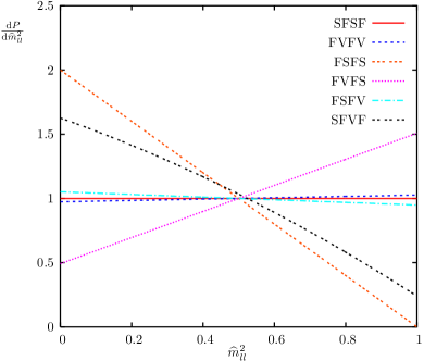
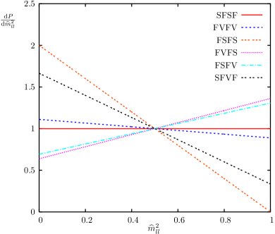
Figure 2: Dilepton mass distributions for (a) mass spectrum I and (b) mass spectrum II.

We see from figure 2 that, as found in [4], the SFSF (SUSY) and FVFV (UED) decay chains would be very hard to distinguish on the basis of the dilepton distribution. On the other hand the FSFS and FVFS cases, where one or both of the UED vector particles is replaced by a scalar, are characteristically different, as is the chain in which one SUSY scalar is replaced by a vector (SFVF). Here and in the discussion of subsequent plots, we shall quantify these initial qualitative observations in section 4.

3.2 Quark and near lepton mass distributions

The quark and near lepton distribution is not experimentally observable as the near and far leptons cannot be distinguished. We can however measure jet $l^{\pm}$ mass distributions, as pointed out in [1]. In order to compute these, we must first calculate the near and far distributions. These are then combined in section 3.4.

The quark and near lepton invariant mass, $m_{ql}^{\rm near}$, is given in terms of the angle between the two particles, $\theta^{*}$, in the rest frame of particle $C$:

$$(m_{ql}^{\rm near})^{2}=\frac{1}{2}(1-x)(1-y)(1-\cos\theta^{*})m_{D}^{2}.$$ (4)

We then define the rescaled invariant mass

$$\widehat{m}_{ql}^{\rm near}=m_{ql}^{\rm near}/(m_{ql}^{\rm near})_{\rm max}=\sin(\theta^{*}/2).$$ (5)

Figure 3 shows the quark and near lepton mass distribution, $\mathrm{d}P/\mathrm{d}(\widehat{m}_{ql}^{\rm near})^{2}$, in process 1 as a function of $(\widehat{m}_{ql}^{\rm near})^{2}$ for mass spectra I and II. Figure 4 shows the same thing for process 2. These are reflections of the distributions for process 1 about the point $(\widehat{m}_{ql}^{\rm near})^{2}=1/2$. The analytical equations for the functions are in appendix B.2.

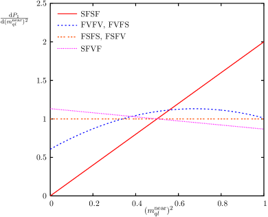
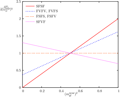
Figure 3: Quark and near lepton mass distributions for process 1 with (a) mass spectrum I and (b) mass spectrum II.

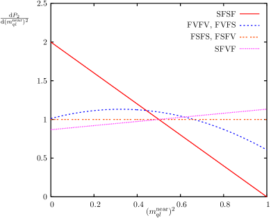
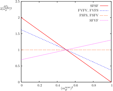
Figure 4: Quark and near lepton mass distributions for process 2 with (a) mass spectrum I and (b) mass spectrum II.

Note that the distributions for FVFV and FVFS and for FSFS and FSFV are the same as the differences in the chains only occur at the last vertex, which has no effect on the quark and near lepton distribution. Furthermore the distribution for FSFS and FSFV is flat since the quark and near lepton are connected by a scalar in these cases. The prospects for distinguishing the remaining cases look quite favourable. However, as remarked above, we must first take account of the contribution of the far lepton.

3.3 Quark and far lepton mass distributions

The quark and far lepton mass is a more complicated expression than the other two. It is a function of all the decay angles in the chain:

$$(m_{ql}^{\rm far})^{2} = \frac{1}{4}(1-x)(1-z)\left[(1+y)(1-\cos\theta^{*}\cos\theta)\right.$$ (6)

$$\quad\left.+(1-y)(\cos\theta^{*}-\cos\theta)-2\sqrt{y}\sin\theta^{*}\sin\theta\cos\phi\right]m_{D}^{2},$$

where $\theta^{*}$ and $\theta$ are as before and $\phi$ is the angle between the $ql^{\rm near}$ and dilepton planes, in the rest frame of $B$. The maximum value is at $\theta^{*}=0$ and $\theta=\pi$ giving

$$(m_{ql}^{\rm far})_{\rm max}^{2}=(1-x)(1-z)m_{D}^{2},$$ (7)

so we define the rescaled mass to be

$$\widehat{m}_{ql}^{\rm far}\equiv(m_{ql}^{\rm far})/(m_{ql}^{\rm far})_{\rm max} = \frac{1}{2}\left[(1+y)(1-\cos\theta^{*}\cos\theta)+\right.$$ (8)

$$\quad\left.(1-y)(\cos\theta^{*}-\cos\theta)-2\sqrt{y}\sin\theta^{*}\sin\theta\cos\phi\right]^{\frac{1}{2}}.$$

Figure 5 shows the quark and far lepton mass distribution, $\mathrm{d}P/\mathrm{d}(\widehat{m}_{ql}^{\rm far})^{2}$, in process 1 as a function of $(\widehat{m}_{ql}^{\rm far})^{2}$ for mass spectra I and II. Figure 6 shows the same thing for process 2. The analytical equations for the functions are in appendix B.3.

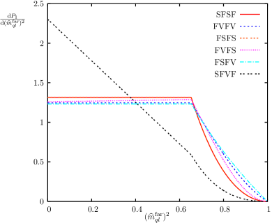
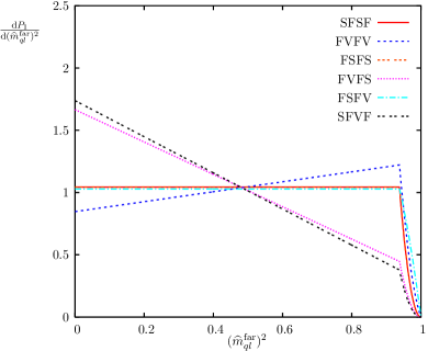
Figure 5: Quark and far lepton mass distributions for process 1 with (a) mass spectrum I and (b) mass spectrum II.

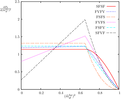
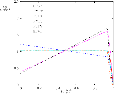
Figure 6: Quark and far lepton mass distributions for process 2 with (a) mass spectrum I and (b) mass spectrum II.

It can be seen from figures 5 and 6, and from the formulae in appendix B.3, that in many cases the dependence on the quark plus far lepton mass is absent or weak throughout the region $0\leq(\widehat{m}_{ql}^{\rm far})^{2}\leq y$. The main exception is SFVF, where the far lepton is connected to the chain via a vector particle. At higher values of $\widehat{m}_{ql}^{\rm far}$, the discrimination is marginally better, which is naturally more useful for spectra with smaller values of $y$ (mass spectrum I). It is clear, however, that the contribution from the far lepton will degrade the power of the quark plus lepton distribution to distinguish between spin assignments.

3.4 Observable quark-lepton mass distribution

We now consider the jet + lepton combinations, $jl^{\pm}$, as first used in [1]. As in [4], we assume that the jet and lepton are indeed decay products from process 1 or process 2. Then the $jl^{\pm}$ mass distribution for a given lepton charge receives near- and far-lepton contributions from both the corresponding process and the charge conjugate of the other process. In other words, we have

$$\frac{\mathrm{d}P}{\mathrm{d}m_{jl^{+}}}=\frac{1}{2}\left[f_{q}\left(\frac{\mathrm{d}P_{2}}{\mathrm{d}m_{ql}^{\rm near}}+\frac{\mathrm{d}P_{1}}{\mathrm{d}m_{ql}^{\rm far}}\right)+f_{\bar{q}}\left(\frac{\mathrm{d}P_{1}}{\mathrm{d}m_{ql}^{\rm near}}+\frac{\mathrm{d}P_{2}}{\mathrm{d}m_{ql}^{\rm far}}\right)\right]$$ (9)

where $f_{q}$ and $f_{\bar{q}}$ are the quark and antiquark fractions in the selected event sample. The factor of one-half enters because $P_{1,2}$ are both normalized to unity. Similarly

$$\frac{\mathrm{d}P}{\mathrm{d}m_{jl^{-}}}=\frac{1}{2}\left[f_{q}\left(\frac{\mathrm{d}P_{1}}{\mathrm{d}m_{ql}^{\rm near}}+\frac{\mathrm{d}P_{2}}{\mathrm{d}m_{ql}^{\rm far}}\right)+f_{\bar{q}}\left(\frac{\mathrm{d}P_{2}}{\mathrm{d}m_{ql}^{\rm near}}+\frac{\mathrm{d}P_{1}}{\mathrm{d}m_{ql}^{\rm far}}\right)\right]\;.$$ (10)

This has assumed that both of the leptons are left-handed – in the case of right-handed leptons, the expressions for $jl^{+}$ and $jl^{-}$ are interchanged.

In [4], the Herwig event generator [16, 17] was used to numerically calculate $f_{q}$ in the cases of SUSY and UED for two different mass spectra. Despite the differences in the models, both gave $f_{q}\approx 0.7$ for both mass spectra. This is therefore the value that we will take for all of our models.

Figures 7 and 8 show the resulting jet+lepton mass distributions for mass spectra I and II, where we have normalised $\widehat{m}_{jl}$ to the maximum observable mass in each case.

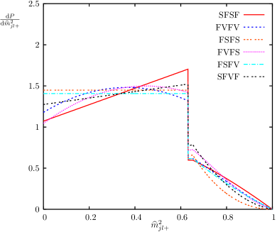
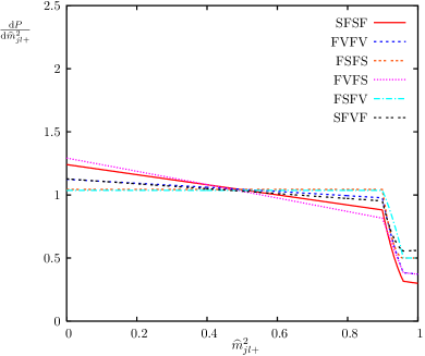
Figure 7: jet$+l^{+}$ mass distribution for (a) mass spectrum I and (b) mass spectrum II.

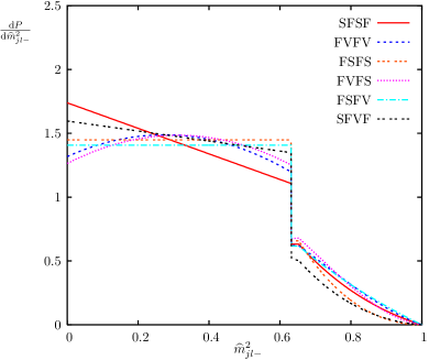
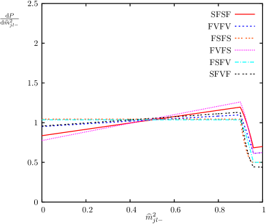
Figure 8: jet$+l^{-}$ mass distribution for (a) mass spectrum I and (b) mass spectrum II.

The resulting charge asymmetry,

$$A=\frac{\mathrm{d}P/\mathrm{d}m_{jl+}-\mathrm{d}P/\mathrm{d}m_{jl-}}{\mathrm{d}P/\mathrm{d}m_{jl+}+\mathrm{d}P/\mathrm{d}m_{jl-}},$$ (11)

is plotted in figure 9. There is a reversal of sign between the predictions for the two mass spectra, since, as discussed in Section 2, the SUSY mass (I) plots assume right-handed leptons, while the UED mass (II) plots assume left.

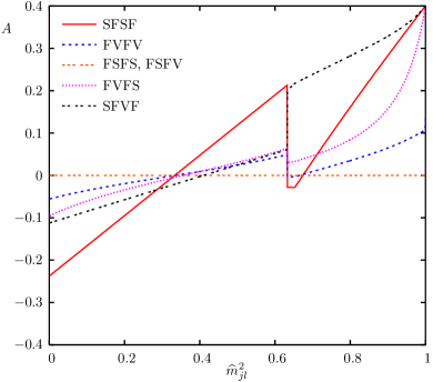
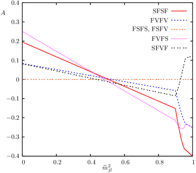
Figure 9: Asymmetry $A$ for (a) mass spectrum I and (b) mass spectrum II.

It is clear from figures 7 and 8 that high statistics would be required to distinguish spin assignments on the basis of the jet plus lepton distributions. This will be seen more quantitatively in section 4. On the other hand, the asymmetries in figure 9 show striking characteristic differences that would provide convincing confirmation of a model once sufficient events had been accumulated.

3.5 Quark, near and far lepton mass distribution

The unscaled $ql^{\rm near}l^{\rm far}$ mass-squared is the sum of the three pairwise unscaled masses-squared already considered:

$$(m_{qll})^{2}=m_{D}^{2}\left[x(1-y)(1-z)(\widehat{m}_{ll})^{2}+(1-x)(1-y)(\widehat{m}_{ql}^{\rm near})^{2}+(1-x)(1-z)(\widehat{m}_{ql}^{\rm far})^{2}\right].$$ (12)

From eqs. (3), (5) and (8), $m_{qll}^{2}$ is a complicated function of the three angles $\theta,\theta^{*}$ and $\phi$. The maximum value of this depends upon the relative values of $x,y$ and $z$. From [12, 13],

$$(m_{qll}^{\rm max})^{2}=\left\{\begin{array}[]{c c}m_{D}^{2}(1-x)(1-yz)&\quad{\rm iff}\quad x<yz,\\ m_{D}^{2}(1-xy)(1-z)&\quad{\rm iff}\quad z<xy,\\ m_{D}^{2}(1-xz)(1-y)&\quad{\rm iff}\quad y<xz,\\ m_{D}^{2}(1-\sqrt{xyz})^{2}&\quad{\rm otherwise.}\end{array}\right.$$ (13)

Both mass spectra I and II have $x<yz$; however, in order to remain independent of the relative values of $x,y$ and $z$, we shall no longer define $\widehat{m}_{qll}$ to lie between 0 and 1. We shall instead simply define

$$\widehat{m}_{qll}=m_{qll}/m_{D},$$ (14)

so that it is still dimensionless.

Figure 10 shows the $qll$ mass distribution, $\mathrm{d}P/\mathrm{d}(\widehat{m}_{qll})^{2}$, for process 1 for mass spectra I and II, while Figure 11 shows the same thing for process 2. The analytical equations are discussed in appendix B.4.

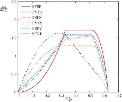
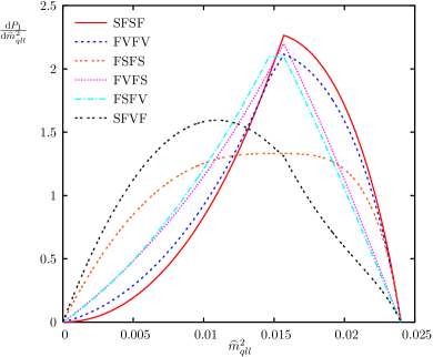
Figure 10: qll mass distributions for process 1 with (a) mass spectrum I and (b) mass spectrum II.

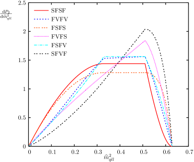
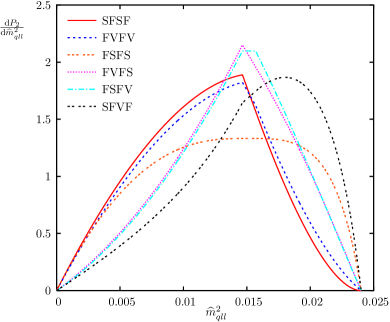
Figure 11: qll mass distributions for process 2 with (a) mass spectrum I and (b) mass spectrum 2.

In an experimental situation we will be unable to distinguish between processes 1 and 2 and will instead see a jet+dilepton distribution that is an equal mixture of the two. The asymmetry between particle and antiparticle production at a $pp$ collider does not help here, because the decays of the unstable particles in the chain into charge conjugate modes must be equal. Figure 12 shows the combined $jll$ plots for mass spectra I and II. We see that there is hope of distinguishing between some cases in the intermediate region of invariant mass.

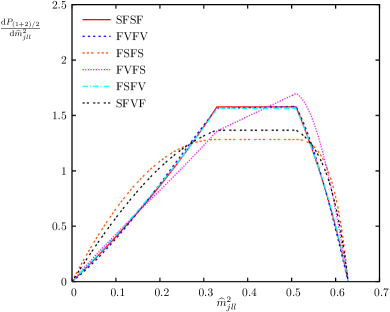
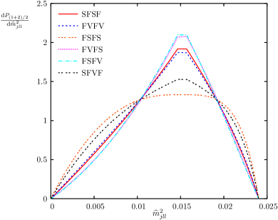
Figure 12: Jet+dilepton mass distributions for Processes 1 and 2 combined for (a) mass spectrum I and (b) mass spectrum II.

4 Model discrimination

It is natural to ask whether from real experimental data it would be possible to determine the underlying set of particle spins present in Nature, given only access to one or more of the invariant mass distributions of section 3. In particular it would be useful to know how many events an experiment would need to identify from one of these decay-chains, in order to favour the assignment of any one spin configuration over any other at a fixed level of confidence. We calculate such a number for each pair of spin configurations and for each distribution (in isolation from the others) assuming a “perfect” detector with infinite acceptance. As real detectors are imperfect and will tend to smear the distributions (thereby losing information) the number of events we calculate should be seen as representing a lower bound on the number of events that a real detector would need to identify.

To calculate the number of events $N$ needed to disfavour a spin configuration $S$ relative to an alternative spin configuration $T$ (which is assumed to be the actual one generating the observed events) we solve the following equation for $N$

$$\frac{1}{R}=\frac{p(S|N{\rm~{}events~{}from~{}}T)}{p(T|N{\rm~{}events~{}from~{}}T)},$$ (15)

in which $R$ is the factor by which configuration $S$ is to be disfavoured with respect to $T$. In this note, $R$ was taken to be 1000. Note that the numerator and the denominator of the right-hand-side of eq. (15) do not transform into each other under the interchange of $S$ and $T$ as a result of $T$’s special role as the true configuration chosen in Nature. This asymmetry is deliberate, reflecting the fact that there will only ever be one underlying distribution which generates the observed events, regardless of the questions which may then be asked of the nature of those events.

4.1 One-dimensional analysis

If we characterise the “$N$ events from $T$” by the $N$ values of a particular invariant mass, $m_{i}^{(T)}$ (for $i\in{1,2,...,N}$), that are observed in those events, then by using Bayes’ Theorem we can rewrite eq. (15) as

$$\frac{1}{R} = \frac{p(S)}{p(T)}\frac{p(N{\rm~{}events~{}from~{}}T|S)}{p(N{\rm~{}events~{}from~{}}T|T)}$$ (16)

$$= \frac{p(S)}{p(T)}\frac{\prod_{i=1}^{N}p(m_{i}^{(T)}|S)}{\prod_{i=1}^{N}p(m_{i}^{(T)}|T)}$$

$$= \frac{p(S)}{p(T)}\exp\left(\sum_{i=1}^{N}{\log\left(\frac{p(m_{i}^{(T)}|S)}{p(m_{i}^{(T)}|T)}\right)}\right).$$

In the limit $N\gg 1$ the sum in eq. (16) may be approximated by an integral over the allowed masses $m^{(T)}$ weighted according to how prevalent they are:

$$\frac{1}{R} \approx \frac{p(S)}{p(T)}\exp\left(N\int_{m}{\log\left(\frac{p(m|S)}{p(m|T)}\right)p(m|T)dm}\right)$$ (17)

$$= \frac{p(S)}{p(T)}\exp\left(-N\int_{m}{\log\left(\frac{p(m|T)}{p(m|S)}\right)p(m|T)dm}\right).$$

The integral in eq. (17) is one that frequently arises in comparisons of distributions [11] and is called the Kullback-Leibler distance of $S$ from $T$, which we shall denote by:

$${\rm KL}(T,S)=\int_{m}{\log\left(\frac{p(m|T)}{p(m|S)}\right)p(m|T)dm}.$$ (18)

Drawing all these threads together we may rearrange eq. (17) to give:

$$N\sim\frac{\log R+\log{\frac{p(S)}{p(T)}}}{{\rm KL}(T,S)}$$ (19)

in the limit of large $N$. Note that the ratio of the prior probabilities for $S$ and $T$ is present in eq. (19) as expected – strong prior evidence for $S$ over $T$ should lead to an increase in the number of events $N$ from one of these chains needed to discredit $S$. For the numbers presented in tables 4 – 7 and discussed in the following section, however, we assign equal prior probabilities to $S$ and $T$, thereby removing all prior dependence from eq. (19). This choice, in effect, looks at the tests in isolation from any pre-existing evidence that might favour $S$ over $T$ or vice versa.

Note that the Kullback-Leibler distance is invariant under diffeomorphisms $m\rightarrow f(m)$ of the distributed variable. This means in particular that the number of events $N$ calculated in eq. (19) does not depend on whether the distributions are considered to be functions of masses or of masses-squared – only the intrinsic information content of the distributions is measured.

4.2 Three-dimensional analysis

To extract the most information from the data we should compare the predictions of different spin assigments with the full probability distribution in the three-dimensional space of $m_{ll}$, $m_{jl^{+}}$ and $m_{jl^{-}}$. The ambiguity between near and far leptons means that this given by

$$P(m_{ll},m_{jl^{+}},m_{jl^{-}}) = \frac{1}{2}f_{q}\left[P_{2}(m_{ll},m_{jl^{+}},m_{jl^{-}})+P_{1}(m_{ll},m_{jl^{-}},m_{jl^{+}})\right]$$ (20)

$$+ \frac{1}{2}f_{\bar{q}}\left[P_{1}(m_{ll},m_{jl^{+}},m_{jl^{-}})+P_{2}(m_{ll},m_{jl^{-}},m_{jl^{+}})\right]\;,$$

where we use $P_{1,2}(m_{ll},m_{jl}^{\rm near},m_{jl}^{\rm far})$ on the right-hand side, assuming both leptons are left-handed, otherwise $f_{q}$ and $f_{\bar{q}}$ are interchanged.

Instead of trying to evaluate the three-dimensional generalization of the integral in eq. (18) analytically, it is convenient to perform a Monte Carlo integration. If we generate $m_{ll}$, $m_{jl}^{\rm near}$ and $m_{jl}^{\rm far}$ according to phase space, the weight to be assigned to the configuration $l^{\rm near}=l^{+}$, $l^{\rm far}=l^{-}$ is

$$P_{+-}(m_{ll},m_{jl}^{\rm near},m_{jl}^{\rm far})=\frac{1}{2}\left[f_{q}P_{2}(m_{ll},m_{jl}^{\rm near},m_{jl}^{\rm far})+f_{\bar{q}}P_{1}(m_{ll},m_{jl}^{\rm near},m_{jl}^{\rm far})\right]$$ (21)

while that for $l^{\rm near}=l^{-}$, $l^{\rm far}=l^{+}$ is

$$P_{-+}(m_{ll},m_{jl}^{\rm near},m_{jl}^{\rm far})=\frac{1}{2}\left[f_{q}P_{1}(m_{ll},m_{jl}^{\rm near},m_{jl}^{\rm far})+f_{\bar{q}}P_{2}(m_{ll},m_{jl}^{\rm near},m_{jl}^{\rm far})\right]\;.$$ (22)

In the former case, since the distinction between $l^{\rm near}$ and $l^{\rm far}$ is lost in the data (except when interchanging them gives a point outside phase space), we must use eq. (20) with $l^{+}=l^{\rm near}$, $l^{-}=l^{\rm far}$ in the logarithmic factor of the KL-distance, i.e. the contribution is

$$\log\left(\frac{P_{+-}(m_{ll},m_{jl}^{\rm near},m_{jl}^{\rm far}|T)+P_{-+}(m_{ll},m_{jl}^{\rm far},m_{jl}^{\rm near}|T)}{P_{+-}(m_{ll},m_{jl}^{\rm near},m_{jl}^{\rm far}|S)+P_{-+}(m_{ll},m_{jl}^{\rm far},m_{jl}^{\rm near}|S)}\right)P_{+-}(m_{ll},m_{jl}^{\rm near},m_{jl}^{\rm far}|T)\;.$$ (23)

Similarly from the configuration $l^{\rm near}=l^{-}$, $l^{\rm far}=l^{+}$ we get the contribution

$$\log\left(\frac{P_{-+}(m_{ll},m_{jl}^{\rm near},m_{jl}^{\rm far}|T)+P_{+-}(m_{ll},m_{jl}^{\rm far},m_{jl}^{\rm near}|T)}{P_{-+}(m_{ll},m_{jl}^{\rm near},m_{jl}^{\rm far}|S)+P_{+-}(m_{ll},m_{jl}^{\rm far},m_{jl}^{\rm near}|S)}\right)P_{-+}(m_{ll},m_{jl}^{\rm near},m_{jl}^{\rm far}|T)\;.$$ (24)

Denoting the sum of these two contributions at the $i$th phase space point by ${\rm KL}_{i}(T,S)$, and summing over $M$ such points, we have as $M\to\infty$

$$\frac{M\log R}{\sum_{i}{\rm KL}_{i}(T,S)}\to N\;,$$ (25)

which is the Monte Carlo equivalent of eq. (19) when the prior probabilities of $S$ and $T$ are taken to be equal. Results for $R=1000$ and $M=5\times 10^{7}$ are shown in table 8 and discussed in the following section.

5 Discussion and conclusions

The results of applying the above one-dimensional analysis to the observable dilepton, jet+lepton and combined jet+dilepton invariant mass distributions separately are presented in tables 4-7, while the results of the three-dimensional analysis are shown in table 8.

(a)	SFSF	FVFV	FSFS	FVFS	FSFV	SFVF
SFSF	$\infty$	60486	23	148	15608	66
FVFV	60622	$\infty$	22	164	6866	62
FSFS	36	34	$\infty$	16	39	266
FVFS	156	173	11	$\infty$	130	24
FSFV	15600	6864	25	122	$\infty$	76
SFVF	78	73	187	27	90	$\infty$

(b)	SFSF	FVFV	FSFS	FVFS	FSFV	SFVF
SFSF	$\infty$	3353	23	304	427	80
FVFV	3361	$\infty$	27	179	232	113
FSFS	36	44	$\infty$	20	22	208
FVFS	313	184	14	$\infty$	13077	35
FSFV	436	236	15	12957	$\infty$	39
SFVF	89	126	134	38	42	$\infty$

Table 4: The number of events needed to disfavour the column model with respect to the row model by a factor of 0.001, assuming the data to come from the row model, for the $\widehat{m}_{ll}^{2}$ distribution (a) mass spectrum I (figure 2a) and (b) mass spectrum II (figure 2b).

(a)	SFSF	FVFV	FSFS	FVFS	FSFV	SFVF
SFSF	$\infty$	1059	205	1524	758	727
FVFV	1090	$\infty$	404	3256	4363	1746
FSFS	278	554	$\infty$	418	741	870
FVFS	1605	3242	345	$\infty$	1256	2365
FSFV	749	4207	507	1212	$\infty$	1803
SFVF	813	1821	751	2415	1888	$\infty$

(b)	SFSF	FVFV	FSFS	FVFS	FSFV	SFVF
SFSF	$\infty$	3006	958	6874	761	1280
FVFV	2961	$\infty$	4427	1685	2749	3761
FSFS	914	4201	$\infty$	743	9874	4877
FVFS	6716	1699	752	$\infty$	656	1306
FSFV	720	2666	10279	649	$\infty$	4138
SFVF	1141	3517	5269	1276	4259	$\infty$

Table 5: As in table 4, for the $\widehat{m}_{jl+}^{2}$ distribution, (a) mass spectrum I (figure 7a) and (b) mass spectrum II (figure 7b).

(a)	SFSF	FVFV	FSFS	FVFS	FSFV	SFVF
SFSF	$\infty$	1058	505	769	816	619
FVFV	1090	$\infty$	541	5878	4821	445
FSFS	565	714	$\infty$	1032	741	2183
FVFS	799	6435	882	$\infty$	2742	510
FSFV	806	4641	507	2451	$\infty$	413
SFVF	692	541	2272	576	521	$\infty$

(b)	SFSF	FVFV	FSFS	FVFS	FSFV	SFVF
SFSF	$\infty$	3037	689	8633	925	967
FVFV	2985	$\infty$	2271	1431	4368	2527
FSFS	707	2297	$\infty$	526	9874	5004
FVFS	8392	1450	525	$\infty$	653	843
FSFV	924	4287	10279	640	$\infty$	4036
SFVF	1047	2693	5213	870	4041	$\infty$

Table 6: As in table 4, for the $\widehat{m}_{jl-}^{2}$ distribution, (a) mass spectrum I (figure 8a) and (b) mass spectrum II (figure 8b).

(a)	SFSF	FVFV	FSFS	FVFS	FSFV	SFVF
SFSF	$\infty$	25630	241	1040	82589	476
FVFV	27315	$\infty$	225	939	14811	432
FSFS	224	204	$\infty$	265	252	2670
FVFS	1009	906	278	$\infty$	1095	504
FSFV	73158	13688	269	1124	$\infty$	557
SFVF	452	400	2749	493	533	$\infty$

(b)	SFSF	FVFV	FSFS	FVFS	FSFV	SFVF
SFSF	$\infty$	26712	189	2213	1686	421
FVFV	26391	$\infty$	224	1323	1073	545
FSFS	182	217	$\infty$	109	101	1710
FVFS	2279	1373	116	$\infty$	46742	210
FSFV	1749	1121	109	47812	$\infty$	193
SFVF	405	528	1712	196	179	$\infty$

Table 7: As in table 4, for the $\widehat{m}_{jll}^{2}$ distribution for processes 1 and 2 combined, (a) mass spectrum I (figure 12a) and (b) mass spectrum II (figure 12b).

(a)	SFSF	FVFV	FSFS	FVFS	FSFV	SFVF
SFSF	$\infty$	455	21	47	348	55
FVFV	474	$\infty$	21	54	1387	55
FSFS	33	34	$\infty$	13	39	188
FVFS	55	67	10	$\infty$	54	19
FSFV	341	1339	25	45	$\infty$	66
SFVF	62	64	143	19	79	$\infty$

(b)	SFSF	FVFV	FSFS	FVFS	FSFV	SFVF
SFSF	$\infty$	1053	21	230	194	63
FVFV	1047	$\infty$	27	135	190	90
FSFS	33	42	$\infty$	19	22	175
FVFS	242	140	13	$\infty$	332	33
FSFV	189	194	14	315	$\infty$	37
SFVF	66	95	118	35	41	$\infty$

Table 8: As in table 4, for the combined three-dimensional distribution. (a) mass spectrum I and (b) mass spectrum II.

As expected from figure 2, the dilepton distribution (table 4) distinguishes very poorly between the spin assignments SFSF (SUSY) and FVFV (UED), even with perfect data, requiring over 60k events for 1:1000 discrimination in the case of mass spectrum I. However, this distribution resolves well between FSFS, FVFS, SFVF and other models.

The jet plus lepton distributions (figures 7, 8 and tables 5, 6) are generally more effective than the dileptons in distinguishing between SFSF and FVFV, but the discrimination is strongly dependent on the mass spectrum. As was emphasised in [4], a ‘quasi-degenerate’ spectrum like II, with large values of the mass ratios $x$, $y$ and $z$ in eq. (1), usually makes it more difficult to resolve between spin assignments. We see however that there are exceptions to this trend, e.g. discrimination between FVFV and FVFS or FSFV.

The jet plus dilepton distribution (figure 12, table 7), like the dileptons alone, proves ineffective in resolving between SFSF and FVFV, but discriminates well between FSFS, SFVF and most other models.

The results in table 8 for the three-dimensional analysis show that, as might be expected, this method achieves a discrimination that is better than that of a one-dimensional analysis applied to any single invariant mass distribution. This could be particularly useful in difficult cases like that of distinguishing between SFSF (SUSY) and FVFV (UED).

We should stress again that the numbers of events in the tables correspond to perfect conditions of signal isolation, resolution and detector efficiency. Realistic conditions would most likely require much higher numbers. Nevertheless, the results obtained provide a guide to the places where attempts to distinguish between spin hypotheses would or would not be worthwhile. Independent of the merits of the hypotheses considered here, the Kullback-Leibler distance (18) is in our view a useful tool for addressing questions of this type.

Appendix A Spin correlations from matrix elements

We give here the analytical formulae for the spin correlations in the cascade decays listed in table 1. For brevity we write $m_{ql}^{\rm near}$ as $m_{qn}$ and $m_{ql}^{\rm far}$ as $m_{qf}$ here, and omit propagator denominators and overall normalization factors. All the distributions presented in this paper are normalized to unity and so such factors are irrelevant. SFSF1 denotes scalar-fermion-scalar-fermion process 1, etc. The mass ratios $x,y,z$ are defined in eq. (1).

SFSF1: $$m^{2}_{qn}$$ (26)

SFSF2: $$(1-x)(1-y)m^{2}_{D}-m^{2}_{qn}$$ (27)

FVFV1: $$x(1-x)y(1-y)(1-z)m^{4}_{D}-2x(1-z)[(y-2xy-4z+2yz)m^{2}_{D}$$ (28)

$$+4zm^{2}_{qn}]m^{2}_{qn}-2x(1-2z)[(1-y)m^{2}_{D}-2m^{2}_{qn}]m^{2}_{qf}$$

$$+(1-2z)[(1-x)(2-y)m^{2}_{D}-2(1-2x)m^{2}_{qn}]m^{2}_{ll}$$

FVFV2: $$x(1-x)(1-y)(1-z)(y+8xz)m^{4}_{D}-8xz(1-z)m^{4}_{qn}$$ (29)

$$-(1-2z)[2x(1-2x)(1-y)m^{2}_{qf}-(1-x)(2-y)m^{2}_{ll}]m^{2}_{D}$$

$$-2\{x(1-z)[y-2(1-2x)(2-y)z]m^{2}_{D}-2x(1-2z)m^{2}_{qf}$$

$$+(1-2z)m^{2}_{ll}\}m^{2}_{qn}$$

FSFS: $$x(1-y)(1-z)m^{2}_{D}-m^{2}_{ll}$$ (30)

FVFS1: $$2\{2xm^{2}_{qf}-(1-2x)[xy(1-z)m^{2}_{D}+m^{2}_{ll}]\}m^{2}_{qn}$$ (31)

$$+\{x(1-y)[(1-x)y(1-z)m^{2}_{D}-2m^{2}_{qf}]+(1-x)(2-y)m^{2}_{ll}\}m^{2}_{D}$$

FVFS2: $$-2[xy(1-z)m^{2}_{D}-2xm^{2}_{qf}+m^{2}_{ll}]m^{2}_{qn}-\{2x(1-2x)(1-y)m^{2}_{qf}$$ (32)

$$-(1-x)[xy(1-y)(1-z)m^{2}_{D}+(2-y)m^{2}_{ll}]\}m^{2}_{D}$$

FSFV: $$x(1-y)(1-z)m^{2}_{D}-(1-2z)m^{2}_{ll}$$ (33)

SFVF1: $$-2x[x(1-y)(2-z)m^{2}_{D}-2m^{2}_{ll}]m^{2}_{qf}+2(1-x)\{2x^{2}y(1-y)(1-z)m^{4}_{D}$$ (34)

$$+[x(1-2y)(2-z)m^{2}_{D}-2m^{2}_{ll}]m^{2}_{ll}\}+xz[x(1-2y)(1-z)m^{2}_{D}$$

$$-2m^{2}_{ll}]m^{2}_{qn}$$

SFVF2: $$-z[x(1-2y)(1-z)m^{2}_{D}-2m^{2}_{ll}]m^{2}_{qn}+2[x(1-y)(2-z)m^{2}_{D}-2m^{2}_{ll}]m^{2}_{qf}$$ (35)

$$+(1-x)z[x(1-y)(1-z)m^{2}_{D}-2m^{2}_{ll}]m^{2}_{D}$$

Appendix B Analytical formulae for invariant mass distributions

This section contains all the analytical formulae for the invariant masses for the 6 chains. Results for the SFSF and FVFV chains have appeared in the literature before [4, 10], but are included here for completeness. Throughout, $m^{2}$ represents the relevant $\widehat{m}^{2}$ for that subsection.

B.1 Dilepton invariant mass distributions

The following table (9) contains the dilepton invariant mass distributions, $\mathrm{d}P/\mathrm{d}m_{ll}^{2}$, for the different chains. These are equal in both processes 1 and 2 and have been normalised to unit area.

Chain	Processes 1 and 2
SFSF	$1$
FVFV	$\frac{2}{(2+y)(1+2z)}(y+4z+(2-y)(1-2z)m^{2})$
FSFS	$2(1-m^{2})$
FVFS	$\frac{2}{2+y}(y+m^{2}(2-y))$
FSFV	$\frac{2}{1+2z}(1-m^{2}(1-2z))$
SFVF	$\frac{3}{(1+2y)(2+z)}(4y+z+4m^{2}(1-y(2-z)-z)-4m^{4}(1-y)(1-z))$

Table 9: Dilepton invariant mass distributions.

B.2 Quark and near lepton invariant mass distributions

The following tables (10 & 11) contain the analytical forms for the quark and near lepton invariant mass distributions, $\mathrm{d}P/\mathrm{d}(m_{ql}^{\rm near})^{2}$. These have been normalised to unit area.

Chain	Process 1
SFSF	$2m^{2}$
FVFV	$\frac{3}{(1+2x)(2+y)}[y+4(1-y+xy)m^{2}-4(1-x)(1-y)m^{4}]$
FSFS	$1$
FVFS	$\frac{3}{(1+2x)(2+y)}[y+4(1-y+xy)m^{2}-4(1-x)(1-y)m^{4}]$
FSFV	$1$
SFVF	$\frac{2(2y+(1-2y)m^{2})}{1+2y}$

Table 10: Quark and near lepton invariant mass distributions for process 1.

Chain	Process 2
SFSF	$2(1-m^{2})$
FVFV	$\frac{3}{(1+2x)(2+y)}[4x+y+4(1-2x-y+xy)m^{2}-4(1-x)(1-y)m^{4}]$
FSFS	$1$
FVFS	$\frac{3}{(1+2x)(2+y)}[4x+y+4(1-2x-y+xy)m^{2}-4(1-x)(1-y)m^{4}]$
FSFV	$1$
SFVF	$\frac{2(1+(-1+2y)m^{2})}{1+2y}$

Table 11: Quark and near lepton invariant mass distributions for process 2.

It is to be expected that the FVFV and FVFS distributions and the FSFS and FSFV distributions match as the chains are identical up to the first two vertices in the chain and the quark and near lepton invariant mass is unaffected by what happens at the third vertex.

B.3 Quark and far lepton invariant mass distributions

The following gives the quark and far lepton invariant mass distributions for the different processes, $\mathrm{d}P/\mathrm{d}(m_{ql}^{\rm far})^{2}$, normalised to unit area. The index 1 or 2 indicates Process 1 or 2 respectively.

SFSF

$$\frac{\mathrm{d}P_{1}}{\mathrm{d}m^{2}}=\frac{-2}{(1-y)^{2}}\left\{\begin{array}[]{l @{\quad} c}(1-y+\log y)&0\leq m^{2}\leq y\\ &\\ (1-m^{2}+\log m^{2})&y\leq m^{2}\leq 1\\ \end{array}\right.$$ (36)

$$\frac{\mathrm{d}P_{2}}{\mathrm{d}m^{2}}=\frac{2}{(1-y)^{2}}\left\{\begin{array}[]{l @{\quad} c}(1-y+y\log y)&0\leq m^{2}\leq y\\ &\\ (1-m^{2}+y\log m^{2})&y\leq m^{2}\leq 1\\ \end{array}\right.$$ (37)

FVFV

$$\frac{\mathrm{d}P_{1}}{\mathrm{d}m^{2}} = \frac{6}{(1+2x)(2+y)(1+2z)(1-y)^{2}}\times$$ (45)

$$\left\{\begin{array}[]{l @{\quad} c}(1-y)[4x-y+2(2+3y-2x(5+y))z&\\ \quad-4m^{2}(2-3x)(1-2z)]-[y(1-2(4+y)z)+4x(2z-y(1-4z))&\\ \qquad+4m^{2}(1+y-x(2+y))(1-2z)]\log y&0\leq m^{2}\leq y\\ &\\ (1-m^{2})[4x(1+2y-5z-6yz)-5y+2(2+9y)z&\\ \quad-4m^{2}(1-x)(1-z)]-[y(1-2(4+y)z)+4x(2z-y(1-4z))&\\ \qquad+4m^{2}(1+y-x(2+y))(1-2z)]\log m^{2}&y\leq m^{2}\leq 1\end{array}\right.$$

$$\frac{\mathrm{d}P_{2}}{\mathrm{d}m^{2}} = \frac{6}{(1+2x)(2+y)(1+2z)(1-y)^{2}}\times$$ (51)

$$\left\{\begin{array}[]{l @{\quad} c}(1-y)[-y+2(2+2x(1-y)+3y)z-4m^{2}(2-x)(1-2z)]&\\ \quad-[y(1-2(4+y)z)+4m^{2}(1+(1-x)y)(1-2z)]\log y&0\leq m^{2}\leq y\\ &\\ (1-m^{2})[4(1+x)z-y(5-18z+8xz)-4m^{2}(1-x)(1-z)]&\\ \quad-[y(1-2(4+y)z)+4m^{2}(1+(1-x)y)(1-2z)]\log m^{2}&y\leq m^{2}\leq 1\\ \end{array}\right.$$

FSFS

$$\frac{\mathrm{d}P_{1,2}}{\mathrm{d}m^{2}}=\frac{-2}{(1-y)^{2}}\left\{\begin{array}[]{l @{\quad} c}(1-y+\log y)&0\leq m^{2}\leq y\\ &\\ (1-m^{2}+\log m^{2})&y\leq m^{2}\leq 1\\ \end{array}\right.$$ (55)

FVFS

$$\frac{\mathrm{d}P_{1}}{\mathrm{d}m^{2}}=\frac{6}{(1+2x)(2+y)(1-y)^{2}}\left\{\begin{array}[]{l @{\quad} c}(1-y)(4x-y-4m^{2}(2-3x))&\\ \quad+[(-1+4x)y&\\ \quad\quad+4m^{2}(2x-1-(1-x)y)]\log y&0\leq m^{2}\leq y\\ &\\ (1-m^{2})(4x-5y+8xy-4m^{2}(1-x))&\\ \quad+[(-1+4x)y&\\ \quad\quad+4m^{2}(2x-1-(1-x)y)]\log m^{2}&y\leq m^{2}\leq 1\\ \end{array}\right.$$ (63)

$$\frac{\mathrm{d}P_{2}}{\mathrm{d}m^{2}}=\frac{6}{(1+2x)(2+y)(1-y)^{2}}\left\{\begin{array}[]{l @{\quad} c}(1-y)(-y-4m^{2}(2-x))&\\ \quad-(y+4m^{2}(1+(1-x)y))\log y&0\leq m^{2}\leq y\\ &\\ (1-m^{2})(-5y-4m^{2}(1-x))&\\ \quad-(y+4m^{2}(1+(1-x)y))\log m^{2}&y\leq m^{2}\leq 1\end{array}\right.$$ (69)

FSFV

$$\frac{\mathrm{d}P_{1,2}}{\mathrm{d}m^{2}}=\frac{-2}{(1+2z)(1-y)^{2}}\left\{\begin{array}[]{l @{\quad} c}(1-y)(1-2z)+(1-2yz)\log y&0\leq m^{2}\leq y\\ &\\ (1-m^{2})(1-2z)+(1-2yz)\log m^{2}&y\leq m^{2}\leq 1\end{array}\right.$$ (73)

SFVF

$$\frac{\mathrm{d}P_{1}}{\mathrm{d}m^{2}}=\frac{6}{(1+2y)(2+z)(1-y)^{2}}\left\{\begin{array}[]{l @{\quad} c}(1-y)(2-3z-2y(1+z)+4m^{2}(1-2z))&\\ \quad-(z+4yz-4m^{2}(1-z-yz))\log y&0\leq m^{2}\leq y\\ &\\ (1-m^{2})(2-3z-8yz+2m^{2}(1-z))&\\ \quad-(z+4yz-4m^{2}(1-z-yz))\log m^{2}&y\leq m^{2}\leq 1\\ \end{array}\right.$$ (74)

$$\frac{\mathrm{d}P_{2}}{\mathrm{d}m^{2}}=\frac{6}{(1+2y)(2+z)(1-y)^{2}}\left\{\begin{array}[]{l @{\quad} c}(1-y)(z-4m^{2}(1-2z))&\\ \quad+(yz-4m^{2}(1-z-yz))\log y&0\leq m^{2}\leq y\\ &\\ (1-m^{2})(z(1+4y)-4m^{2}(1-z))&\\ \quad+(yz-4m^{2}(1-z-yz))\log m^{2}&y\leq m^{2}\leq 1\\ \end{array}\right.$$ (75)

B.4 Quark, near and far lepton mass distributions

Due to the complicated nature of the $qll$ mass, these distributions can be lengthy and complicated. Included in this section are the ones of manageable length - FSFS, FSFV and SFSF (processes 1 and 2). The others are available from the authors on request.

These distributions are given in terms of

$$\mathcal{M}_{ll}^{+}=\mathrm{min}\left\{\begin{array}[]{c}\frac{\frac{1}{4}(1-x)\left(\sqrt{(1-\sqrt{xyz})^{2}-\hat{m}_{qll}^{2}}+\sqrt{(1+\sqrt{xyz})^{2}-\hat{m}_{qll}^{2}}\right)^{2}-(1-x-\hat{m}_{qll}^{2})}{x(1-y)(1-z)}\\ \\ 1.\end{array}\right.$$ (76)

This is equal to 1 in the region between $(1-y)(1-xz)$ and $(1-z)(1-xy)$, which leads to the flat section of the distributions observed. These distributions require the positive constants $\mathcal{N}_{i}$ to be set such that the distribution integrates to 1 in each case.

FSFS

$$\frac{\mathrm{d}P}{\mathrm{d}\hat{m}_{qll}^{2}} = \frac{\mathcal{N}_{1}}{(1-y)^{2}(1-z)^{2}}\Bigg{\{}$$

$$\quad(1-yz)-\sqrt{((1+\sqrt{yz})^{2}-(1-y)(1-z)\mathcal{M}_{ll}^{+})((1-\sqrt{yz})^{2}-(1-y)(1-z)\mathcal{M}_{ll}^{+})}$$

$$-2(y+z)\log{\left(\frac{\sqrt{(1+\sqrt{yz})^{2}-(1-y)(1-z)\mathcal{M}_{ll}^{+}}-\sqrt{(1-\sqrt{yz})^{2}-(1-y)(1-z)\mathcal{M}_{ll}^{+}}}{2\sqrt{yz}}\right)}\Bigg{\}}.$$

FSFV

$$\frac{\mathrm{d}P}{\mathrm{d}\hat{m}_{qll}^{2}} = \frac{\mathcal{N}_{2}}{(1-y)^{2}(1-z)^{2}}\Bigg{\{}(1-2z)(1-yz)$$

$$\quad-(1-2z)\sqrt{((1+\sqrt{yz})^{2}-(1-y)(1-z)\mathcal{M}_{ll}^{+})((1-\sqrt{yz})^{2}-(1-y)(1-z)\mathcal{M}_{ll}^{+})}$$

$$\quad-2(y+z-2z(1+yz))\times$$

$$\quad\log{\left(\frac{\sqrt{(1+\sqrt{yz})^{2}-(1-y)(1-z)\mathcal{M}_{ll}^{+}}-\sqrt{(1-\sqrt{yz})^{2}-(1-y)(1-z)\mathcal{M}_{ll}^{+}}}{2\sqrt{yz}}\right)}\Bigg{\}}.$$

SFSF

$$\frac{\mathrm{d}P_{1}}{\mathrm{d}\hat{m}_{qll}^{2}} = \frac{\mathcal{-N}_{3}}{(1-y)^{2}(1-x)(1-z)}\Bigg{\{}\frac{1}{z}((1+xz)(1-yz)-\hat{m}_{qll}^{2}(1-z))$$

$$\quad+\frac{\mathcal{M}_{ll}^{+}(1-y)(1-z)((1+xz)(1+yz)+2z(1+xy)-\hat{m}_{qll}^{2}(1+z))}{z\sqrt{(1-\sqrt{yz})^{2}-\mathcal{M}_{ll}^{+}(1-y)(1-z)}\sqrt{(1+\sqrt{yz})^{2}-\mathcal{M}_{ll}^{+}(1-y)(1-z)}}$$

$$\quad+\frac{(1-yz)(\hat{m}_{qll}^{2}(1-z)-(1+xz)(1-yz))}{z\sqrt{(1-\sqrt{yz})^{2}-\mathcal{M}_{ll}^{+}(1-y)(1-z)}\sqrt{(1+\sqrt{yz})^{2}-\mathcal{M}_{ll}^{+}(1-y)(1-z)}}$$

$$\quad-4(1+xy)\log{\left(\frac{\sqrt{(1+\sqrt{yz})^{2}-(1-y)(1-z)\mathcal{M}_{ll}^{+}}-\sqrt{(1-\sqrt{yz})^{2}-(1-y)(1-z)\mathcal{M}_{ll}^{+}}}{2\sqrt{yz}}\right)}\Bigg{\}}.$$

$$\frac{\mathrm{d}P_{2}}{\mathrm{d}\hat{m}_{qll}^{2}} = -\frac{\mathrm{d}P_{1}}{\mathrm{d}\hat{m}_{qll}^{2}}$$

$$+\frac{8\mathcal{N}_{3}}{(1-y)(1-z)}\log{\left(\frac{\sqrt{(1+\sqrt{yz})^{2}-(1-y)(1-z)\mathcal{M}_{ll}^{+}}-\sqrt{(1-\sqrt{yz})^{2}-(1-y)(1-z)\mathcal{M}_{ll}^{+}}}{2\sqrt{yz}}\right)}\Bigg{\}}$$

An explicitly normalised expression for an equal mixture of process 1 and process 2 for the SFSF (supersymmetric) spin configuration may be found in [18].

References

• [1] A. J. Barr, “Using lepton charge asymmetry to investigate the spin of supersymmetric particles at the LHC,” Phys. Lett. B596 (2004) 205–212, hep-ph/0405052.
• [2] T. Goto, K. Kawagoe, and M. M. Nojiri, “Study of the slepton non-universality at the CERN Large Hadron Collider,” Phys. Rev. D70 (2004) 075016, hep-ph/0406317.
• [3] H. C. Cheng, K. T. Matchev and M. Schmaltz, “ Bosonic supersymmetry? Getting fooled at the LHC,” Phys. Rev. D66 (2002) 056006, hep-ph/0205314.
• [4] J. M. Smillie and B. R. Webber, “Distinguishing spins in supersymmetric and universal extra dimension models at the Large Hadron Collider,” JHEP 10 (2005) 069, hep-ph/0507170.
• [5] M. Battaglia, A. Datta, A. De Roeck, K. Kong, and K. T. Matchev, “Contrasting supersymmetry and universal extra dimensions at the CLIC multi-TeV e+ e- collider,” JHEP 07 (2005) 033, hep-ph/0502041.
• [6] A. Datta, K. Kong, and K. T. Matchev, “Discrimination of supersymmetry and universal extra dimensions at hadron colliders,” Phys. Rev. D72 (2005) 096006, hep-ph/0509246.
• [7] A. Datta, G. L. Kane, and M. Toharia, “Is it SUSY?,” hep-ph/0510204.
• [8] A. J. Barr, “Measuring slepton spin at the LHC,” JHEP 02 (2006) 042, hep-ph/0511115.
• [9] A. Alves, O. Eboli, and T. Plehn, “It’s a gluino,” hep-ph/0605067.
• [10] D. J. Miller, P. Osland, and A. R. Raklev, “Invariant mass distributions in cascade decays,” hep-ph/0510356.
• [11] S. Kullback and R. A. Leibler, “On information and sufficiency,” Annals of Mathematical Statistics 22(1) (1951) 79–86.
• [12] B. C. Allanach, C. G. Lester, M. A. Parker, and B. R. Webber, “Measuring sparticle masses in non-universal string inspired models at the LHC,” JHEP 09 (2000) 004, hep-ph/0007009.
• [13] C. G. Lester, “Model independent sparticle mass measurements at ATLAS,”. CERN-THESIS-2004-003.
• [14] B. C. Allanach et al., “The Snowmass points and slopes: Benchmarks for SUSY searches,” Eur. Phys. J. C25 (2002) 113–123, hep-ph/0202233.
• [15] H.-C. Cheng, K. T. Matchev, and M. Schmaltz, “Radiative corrections to Kaluza-Klein masses,” Phys. Rev. D66 (2002) 036005, hep-ph/0204342.
• [16] G. Corcella et al., “HERWIG 6: An event generator for hadron emission reactions with interfering gluons (including supersymmetric processes),” JHEP 01 (2001) 010, hep-ph/0011363.
• [17] G. Corcella et al., “HERWIG 6.5 release note,” hep-ph/0210213.
• [18] C. G. Lester, “Constrained invariant mass distributions in cascade decays: The shape of the ’m(qll)-threshold’ and similar distributions,” hep-ph/0603171.