Generalized form factors, generalized parton distributions
and the spin contents of the nucleon

Abstract

With a special intention of clarifying the underlying spin contents of the nucleon, we investigate the generalized form factors of the nucleon, which are defined as the $n$-th $x$-moments of the generalized parton distribution functions, within the framework of the chiral quark soliton model. A particular emphasis is put on the pion mass dependence of final predictions, which we shall compare with the predictions of lattice QCD simulations carried out in the so-called heavy pion region around $m_{\pi}\simeq(700\sim 900)\,\mbox{MeV}$. We find that some observables are very sensitive to the variation of the pion mass. It will be argued that the negligible importance of the quark orbital angular momentum indicated by the LHPC and QCDSF lattice collaborations might be true in the unrealistic heavy pion world, but it is not necessarily the case in our real world close to the chiral limit.

I Introduction

The so-called “nucleon spin crisis” raised by the European Muon Collaboration (EMC) measurement in 1988 is one of the most outstanding findings in the field of hadron physics EMC88 ,EMC89 . The renaissance of the physics of high energy deep inelastic scatterings is greatly indebted to this epoch-making finding. Probably, one of the most outstanding progresses achieved recently in this field of physics is the discovery and the subsequent research of completely new observables called generalized parton distribution functions (GPD). It has been revealed that the GPDs, which can be measured through the so-called deeply-virtual Compton scatterings (DVCS) or the deeply-virtual meson productions (DVMP), contain surprisingly richer information than the standard parton distribution functions MRGDH94 –RP02 .

Roughly speaking, the GPDs are generalization of ordinary parton distributions and the elastic form factors of the nucleon. The GPDs in the most general form are functions of three kinematical variables : the average longitudinal momentum fraction $x$ of the struck parton in the initial and final states, a skewdness parameter $\xi$ which measures the difference between two momentum fractions, and the four-momentum-transfer square $t$ of the initial and final nucleon. In the forward limit $t\rightarrow 0$, some of the GPDs reduce to the usual quark, antiquark and gluon distributions. On the other hand, taking the $n$-th moment of the GPDs with respect to the variable $x$, one obtains the generalizations of the electromagnetic form factors of the nucleon, which are called the generalized form factors of the nucleon. The complex nature of the GPDs, i.e. the fact that they are functions of three variable, makes it quite difficult to grasp their full characteristics both experimentally and theoretically. From the theoretical viewpoint, it may be practical to begin studies with the two limiting cases. The one is the forward limit of zero momentum transfer. We have mentioned that, in this limit, some of the GPDs reduce to the ordinary parton distribution function depending on one variable $x$. However, it turns out that, even in this limit, there appear some completely new distribution functions, which cannot be accessed by the ordinary inclusive deep-inelastic scattering measurements. Very interestingly, it was shown by Ji that one of such distributions contains valuable information on the total angular momentum carried by the quark fields in the nucleon Ji97 –JTH96 . This information, combined with the known knowledge on the longitudinal quark polarization, makes it possible to determine the quark orbital angular momentum contribution to the total nucleon spin purely experimentally.

Another relatively-easy-to-handle quantities are the generalized form factors of the nucleon DFJK05 ,Diehl05 , which are given as the non-forward nucleon matrix elements of the spin-$n$, twist-two quark and gluon operators. Since these latter quantities are given as the nucleon matrix elements of local operators, they can be objects of lattice QCD simulations. (It should be compared with parton distributions. The direct calculation of parton distributions is beyond the scope of lattice QCD simulations, since it needs to treat the nucleon matrix elements of quark bilinears, which are nonlocal in time.) In fact, two groups, the LHPC collaboration and the QCDSF collaboration independently investigated the generalized form factors of the nucleon, and gave several interesting predictions, which can in principle be tested by the measurement of GPDs in the near future LHPC02 –QCDSF05 . Although interesting, there is no a priori reason to believe that the predictions of these lattice simulations are realistic enough. The reason is mainly that the above mentioned lattice simulation were carried out in the heavy pion regime around $m_{\pi}\simeq(700\sim 900)\,\mbox{MeV}$ with neglect of the so-called disconnected diagrams. Our real world is rather close to the chiral limit with vanishing pion mass, and we know that, in this limit, the Goldstone pion plays very important roles in some intrinsic properties of the nucleon. The lattice simulation carried out in the heavy pion region is in danger of missing some important role of chiral dynamics.

On the other hand, the chiral quark soliton model (CQSM) is an effective model of baryons, which maximally incorporates the chiral symmetry of QCD and its spontaneous breakdown DPP88 ,WY91 . (See Wakamatsu92R –ARW96 for early reviews.) It was already applied to the physics of ordinary parton distribution functions with remarkable success WGR96 –Wakamatsu03b . For instance, an indispensable role of pion-like quark-antiquark correlation was shown to be essential to understand the famous NMC measurement, which revealed the dominance of the $\bar{d}$-quark over the $\bar{u}$-quark inside the proton WK98 ,PPGWW99 ,Wakamatsu92 . Then, it would be interesting to see what predictions the CQSM would give for the quantities mentioned above. Now, the main purpose of the present study is to study the generalized form factors of the nucleon within the framework of the CQSM and compare its predictions with those of the lattice QCD simulations. Of our particular interest here is to see the change of final theoretical predictions against the variation of the pion mass. Such an analysis is expected to give some hints for judging the reliability of the lattice QCD predictions at the present level for the observables in question.

The plan of the paper is as follows. In sect.II, we shall briefly explain how to introduce the nonzero pion mass into the scheme of the CQSM with Pauli-Villars regularization. In sect.III, we derive the theoretical expressions for the generalized form factors of the nucleon. Sect.IV is devoted to the discussion of the results of the numerical calculations. Some concluding remarks are then given in sect.V.

II Model lagrangian with pion mass term

We start with the basic effective lagrangian of the chiral quark soliton model in the chiral limit given as

$${\cal L}_{0}=\bar{\psi}(x)(i\not\!\partial-MU^{\gamma_{5}}(x))\psi(x),$$ (1)

with

$$U^{\gamma_{5}}(x)\ =\ e^{i\gamma_{5}\mbox{\boldmath$\tau$}\cdot\mbox{\boldmath$\pi$}(x)/f_{\pi}}\ =\ \frac{1+\gamma_{5}}{2}\,U(x)+\frac{1-\gamma_{5}}{2}\,U^{\dagger}(x).$$ (2)

which describes the effective quark fields, with a dynamically generated mass $M$, strongly interacting with pions DPP88 ,WY91 . Since one of the main purposes of the present study is to see how the relevant observables depend on pion mass, we add to ${\cal L}_{0}$ an explicit chiral symmetry breaking term ${\cal L}^{\prime}$ given by KWW99

$${\cal L}^{\prime}=\frac{1}{4}\,f_{\pi}^{2}\,m_{\pi}^{2}\,\mbox{tr}_{f}\,[U(x)+U^{\dagger}(x)-2].$$ (3)

Here the trace in (3) is to be taken with respect to flavor indices. The total model lagrangian is therefore given by

$${\cal L}_{CQM}={\cal L}_{0}+{\cal L}^{\prime}.$$ (4)

Naturally, one could have taken an alternative choice in which the explicit chiral-symmetry-breaking effect is introduced in the form of current quark mass term as ${\cal L}^{\prime}=-m_{0}\bar{\psi}\psi$. We did not do so, because we do not know any consistent regularization of such effective lagrangian with finite current quark mass within the framework of the Pauli-Villars subtraction scheme, as explained in Appendix of KWW99 . The effective action corresponding to the above lagrangian is given as

$$S_{eff}[U]=S_{F}[U]+S_{M}[U],$$ (5)

with

$$S_{F}[U]=-\,i\,N_{c}\,\mbox{Sp}\,\ln(i\not\!\partial-MU^{\gamma_{5}}),$$ (6)

and

$$S_{M}[U]=\int\frac{1}{4}\,f_{\pi}^{2}\,m_{\pi}^{2}\,\mbox{tr}_{f}\,[U(x)+U^{\dagger}(x)-2]\,d^{4}x.$$ (7)

Here $\mbox{Sp}\hat{O}=\int d^{4}x\,\mbox{tr}_{\gamma}\,\mbox{tr}_{f}\,\langle x|\hat{O}|x\rangle$ with $\mbox{tr}_{\gamma}$ and $\mbox{tr}_{f}$ representing the trace of the Dirac gamma matrices and the flavors (isospins), respectively. The fermion (quark) part of the above action contains ultra-violet divergences. To remove these divergences, we must introduce physical cutoffs. For the purpose of regularization, here we use the Pauli-Villars subtraction scheme. As explained in KWW99 , we must eliminate not only the logarithmic divergence contained in $S_{f}[U]$ but also the quadratic and logarithmic divergence contained in the equation of motion shown below. To get rid of all these troublesome divergence, we need at least two subtraction terms. The regularized action is thus defined as

$$S_{eff}^{reg}[U]=S_{F}^{reg}[U]+S_{M}[U],$$ (8)

where

$$S_{F}^{reg}[U]=S_{F}[U]-\sum_{i=1}^{2}\,c_{i}\,S_{F}^{\Lambda_{i}}[U].$$ (9)

Here $S_{F}^{\Lambda_{i}}$ is obtained from $S_{F}[U]$ with $M$ replaced by the Pauli-Villars regulator mass $\Lambda_{i}$. These parameters are fixed as follows. First, the quadratic and logarithmic divergence contained in the equation of motion (or in the expression of the vacuum quark condensate) can, respectively, removed if the subtraction constants satisfy the following two conditions :

$$M^{2} - \sum_{i=1}^{2}c_{i}\Lambda_{i}^{2}=0,$$ (10)

$$M^{4} - \sum_{i=1}^{2}c_{i}\Lambda_{i}^{4}=0.$$ (11)

(We recall that the condition which removes the logarithmic divergence in $S_{f}[U]$ just coincides with the 1st of the above conditions.) By solving the above equations for $c_{1}$ and $c_{2}$, we obtain

$$c_{1} = \left(\frac{M}{\Lambda_{1}}\right)^{2}\frac{\Lambda_{2}^{2}-M^{2}}{\Lambda_{2}^{2}-\Lambda_{1}^{2}},$$ (12)

$$c_{2} = -\left(\frac{M}{\Lambda_{2}}\right)^{2}\frac{\Lambda_{1}^{2}-M^{2}}{\Lambda_{2}^{2}-\Lambda_{1}^{2}},$$ (13)

which constrains the values of $c_{1}$ and $c_{2}$, once $\Lambda_{1}$ and $\Lambda_{2}$ are given. For determining $\Lambda_{1}$ and $\Lambda_{2}$, we use two conditions

$$\frac{N_{c}M^{2}}{4\pi^{2}}\,\sum_{i=1}^{2}\,c_{i}\,\left(\frac{\Lambda_{i}}{M}\right)^{2}\,\ln\left(\frac{\Lambda_{i}}{M}\right)^{2}=f_{\pi}^{2},$$ (14)

and

$$\langle\bar{\psi}\psi\rangle_{vac}=\frac{N_{c}M^{3}}{2\pi^{2}}\,\sum_{i=1}^{2}\,c_{i}\,\left(\frac{\Lambda_{i}}{M}\right)^{4}\ln\left(\frac{\Lambda_{i}}{M}\right)^{4},$$ (15)

which amounts to reproducing the correct normalization of the pion kinetic term in the effective meson lagrangian and also the empirical value of the vacuum quark condensate. To derive soliton equation of motion, we must first write down a regularized expression for the static soliton energy. Under the hedgehog ansatz $\mbox{\boldmath$\pi$}(\mbox{\boldmath$x$})=f_{\pi}\hat{\mbox{\boldmath$r$}}F(r)$ for the background pion fields, it is obtained in the form :

$$E_{static}^{reg}[F(r)]=E_{F}^{reg}[F(r)]+E_{M}[F(r)],$$ (16)

where the meson (pion) part is given by

$$E_{M}[F(r)]=-\,f_{\pi}^{2}\,m_{\pi}^{2}\int d^{3}x\,[\cos F(r)-1],$$ (17)

while the fermion (quark) part is given as

$$E_{F}^{reg}[F(r)]=E_{val}+E_{vp}^{reg},$$ (18)

with

$$E_{val} = N_{c}\,E_{0},$$ (19)

$$E_{vp}^{reg} = N_{c}\,\sum_{n<0}\,(E_{n}-E_{n}^{(0)})-\sum_{i=1}^{N}\,c_{i}\,N_{c}\,\sum_{n<0}\,(E_{n}^{\Lambda_{i}}-E_{n}^{(0)\Lambda_{i}}).$$ (20)

Here $E_{n}$ are the quark single-particle energies, given as the eigenvalues of the static Dirac Hamiltonian in the background pion fields :

$$H\,|n\rangle=E_{n}|n\rangle,$$ (21)

with

$$H=\frac{\mbox{\boldmath$\alpha$}\cdot\nabla}{i}+\beta M\,[\cos F(r)+i\gamma_{5}\mbox{\boldmath$\tau$}\cdot\hat{\mbox{\boldmath$r$}}\sin F(r)],$$ (22)

while $E_{n}^{(0)}$ denote energy eigenvalues of the vacuum Hamiltonian given by (22) with $F(r)=0$ (or $U=1$). The particular state $|n=0\rangle$, which is a discrete bound-state orbital coming from the upper Dirac continuum under the influence of the hedgehog mean field, is called the valence level. The symbol $\sum_{n<0}$ in (20) denotes the summation over all the negative energy eigenstates of $H$, i.e. the negative energy Dirac continuum. The soliton equation of motion is obtained from the stationary condition of $E_{static}^{reg}[F(r)]$ with respect to the variation of the profile function $F(r)$ :

$$0 = \frac{\delta}{\delta F(r)}\,E_{static}[F(r)]$$ (23)

$$= 4\pi r^{2}\,\left\{-\,M\,[S(r)\sin F(r)-P(r)\cos F(r)]+f_{\pi}^{2}m_{\pi}^{2}\sin F(r)\right\},$$

which gives

$$F(r)=\arctan\left(\frac{P(r)}{S(r)-f_{\pi}^{2}m_{\pi}^{2}/M}\right).$$ (24)

Here $S(r)$ and $P(r)$ are regularized scalar and pseudoscalar quark densities given as

$$S(r) = S_{val}(r)+\sum_{n<0}S_{n}(r)-\sum_{i=1}^{2}\,c_{i}\,\frac{\Lambda_{i}}{M}\,\sum_{n<0}\,S_{n}^{\Lambda_{i}}(r),$$ (25)

$$P(r) = P_{val}(r)+\sum_{n<0}P_{n}(r)-\sum_{i=1}^{2}\,c_{i}\,\frac{\Lambda_{i}}{M}\,\sum_{n<0}\,P_{n}^{\Lambda_{i}}(r),$$ (26)

with

$$S_{n}(r) = \frac{N_{c}}{4\pi}\int d^{3}x\,\,\langle n|\mbox{\boldmath$x$}\rangle\,\gamma^{0}\,\frac{\delta(|\mbox{\boldmath$x$}|-r)}{r^{2}}\,\langle\mbox{\boldmath$x$}|n\rangle,$$ (27)

$$P_{n}(r) = \frac{N_{c}}{4\pi}\int d^{3}x\,\langle n|\mbox{\boldmath$x$}\rangle\,i\,\gamma^{0}\,\gamma_{5}\,\mbox{\boldmath$\tau$}\cdot\hat{\mbox{\boldmath$r$}}\,\frac{\delta(|\mbox{\boldmath$x$}|-r)}{r^{2}}\langle\mbox{\boldmath$x$}|n\rangle,$$ (28)

while $S_{n}^{\Lambda_{i}}(r)$ and $P_{n}^{\Lambda_{i}}(r)$ are the corresponding densities evaluated with the regulator mass $\Lambda_{i}$ instead of the dynamical quark mass $M$. We also note that $S_{val}(r)\equiv S_{n=0}(r)$ and $P_{val}(r)\equiv P_{n=0}(r)$. As usual, a self-consistent soliton solution is obtained as follows with use of Kahana and Ripka’s discretized momentum basis KR84 ,KRS84 . First by assuming an appropriate (though arbitrary) soliton profile $F(r)$, the eigenvalue problem of the Dirac Hamiltonian is solved. Using the resultant eigenfunctions and their associated eigenenergies, one can calculate the regularized scalar and pseudoscalar densities $S(r)$ and $P(r)$. With use of these $S(r)$ and $P(r)$, Eq.(24) can then be used to obtain a new soliton profile $F(r)$. The whole procedure above is repeated with this new profile $F(r)$ until the self-consistency is attained.

III Generalized Form Factors in the CQSM

Since the generalized form factors of the nucleon are given as moments of generalized parton distributions (GPDs), it is convenient to start with the theoretical expressions of the unpolarized GPDs $H(x,\xi,t)$ and $E(x,\xi,t)$ within the CQSM. Following the notation in Ossmann05 ,WT05 , we introduce the quantities

$${\cal M}_{s^{\prime}s}^{(I=0)}\equiv\int\frac{d\lambda}{2\pi}\,e^{i\lambda x}\,\langle\mbox{\boldmath$p$}^{\prime},s^{\prime}|\,\bar{\psi}\left(-\frac{\lambda n}{2}\right)\not\!n\psi\left(\frac{\lambda n}{2}\right)|\mbox{\boldmath$p$},s\rangle,$$ (29)

and

$${\cal M}_{s^{\prime}s}^{(I=1)}\equiv\int\frac{d\lambda}{2\pi}\,e^{i\lambda x}\,\langle\mbox{\boldmath$p$}^{\prime},s^{\prime}|\,\bar{\psi}\left(-\frac{\lambda n}{2}\right)\tau_{3}\not\!n\psi\left(\frac{\lambda n}{2}\right)|\mbox{\boldmath$p$},s\rangle.$$ (30)

Here, the isoscalar and isovector combinations respectively correspond to the sum and the difference of the quark flavors $u$ and $d$. The relation between these quantities and the generalized parton distribution functions $H(x,\xi,t)$ and $E(x,\xi,t)$ are obtained most conveniently in the so-called Breit frame. They are given by

$${\cal M}_{s^{\prime}s}^{(I=0)} = 2\,\delta_{s^{\prime}s}\,H_{E}^{(I=0)}(x,\xi,t)\ -\ \frac{i\,\varepsilon^{3kl}\,\Delta^{k}}{M_{N}}\,(\sigma^{l})_{s^{\prime}s}\,E_{M}^{(I=0)}(x,\xi,t),$$ (31)

$${\cal M}_{s^{\prime}s}^{(I=1)} = 2\,\delta_{s^{\prime}s}\,H_{E}^{(I=1)}(x,\xi,t)\ -\ \frac{i\,\varepsilon^{3kl}\,\Delta^{k}}{M_{N}}\,(\sigma^{l})_{s^{\prime}s}\,E_{M}^{(I=1)}(x,\xi,t).$$ (32)

where

$$H_{E}^{(I=0/1)}(x,\xi,t) \equiv H^{(I=0/1)}(x,\xi,t)+\frac{t}{4M_{N}^{2}}E^{(I=0/1)}(x,\xi,t),$$ (33)

$$E_{M}^{(I=0/1)}(x,\xi,t) \equiv H^{(I=0/1)}(x,\xi,t)+E^{(I=0/1)}(x,\xi,t).$$ (34)

These two independent combinations of $H(x,\xi,t)$ and $E(x,\xi,t)$ can be extracted through the spin projection of ${\cal M}^{(I=0/1)}$ as

$$H_{E}^{(I)}(x,\xi,t) = \frac{1}{4}\,\mbox{tr}\{{\cal M}^{(I)}\},$$ (35)

$$E_{M}^{(I)}(x,\xi,t) = \frac{i\,M_{N}\,\varepsilon^{3bm}\,\Delta^{b}}{2\mbox{\boldmath$\Delta$}_{\perp}^{2}}\,\mbox{tr}\{\sigma^{m}{\cal M}^{(I)}\},$$ (36)

where “tr” denotes the trace over spin indices, while $\mbox{\boldmath$\Delta$}_{\perp}^{2}=\mbox{\boldmath$\Delta$}^{2}-(\Delta^{3})^{2}=-t-(-2M_{N}\xi)^{2}$. Now, within the CQSM, it is possible to evaluate the right-hand side (rhs) of (35) and (36). Since the answers are already given in several previous papers Ossmann05 –Petrov98 , we do not repeat the derivation. Here we comment only on the following general structure of the theoretical expressions for relevant observables in the CQSM. The leading contribution just corresponds to the mean field prediction, which is independent of the collective rotational velocity $\Omega$ of the hedgehog soliton. The next-to-leading order term takes account of the linear response of the internal quark motion to the rotational motion as an external perturbation, and consequently it is proportional to $\Omega$. It is known that the leading-order term contributes to the isoscalar combination of $H_{E}(x,\xi,t)$ and to the isovector combination of $E_{M}(x,\xi,t)$, while the isoscalar part of $H_{E}(x,\xi,t)$ and the isovector part of $E_{M}(x,\xi,t)$ survived only at the next-to-leading order of $\Omega$ (or of $1/N_{c}$). The leading-order GPDs are then given as

$$H_{E}^{(I=0)}(x,\xi,t) = M_{N}N_{c}\int\frac{dz^{0}}{2\pi}\,\sum_{n\leq 0}\,e^{iz^{0}(xM_{N}-E_{n})}\int d^{3}\mbox{\boldmath$x$}\,\Phi_{n}^{\dagger}(\mbox{\boldmath$x$})$$ (37)

$$\times\ (1+\gamma^{0}\gamma^{3})\,e^{-i(z^{0}/2)\hat{p}_{3}}\,e^{i\mbox{\boldmath$\Delta$}\cdot\mbox{\boldmath$x$}}\,e^{-i(z^{0}/2)\hat{p}_{3}}\,\Phi_{n}(\mbox{\boldmath$x$}),$$

$$E_{M}^{(I=1)}(x,\xi,t) = \frac{2\,i\,M_{N}^{2}\,N_{c}}{3\,(\mbox{\boldmath$\Delta$}_{\perp})^{2}}\int\frac{dz^{0}}{2\pi}\,\sum_{n\leq 0}\,e^{iz^{0}(xM_{N}-E_{n})}\,\int d^{3}\mbox{\boldmath$x$}\,\Phi_{n}^{\dagger}(\mbox{\boldmath$x$})$$ (38)

$$\times\ (1+\gamma^{0}\gamma^{3})\,(\mbox{\boldmath$\tau$}\times\mbox{\boldmath$\Delta$})^{3}\,e^{-i(z^{0}/2)\hat{p}_{3}}\,e^{i\mbox{\boldmath$\Delta$}\cdot\mbox{\boldmath$x$}}\,e^{-i(z^{0}/2)\hat{p}_{3}}\,\Phi_{n}(\mbox{\boldmath$x$}).$$

Here the symbol $\Sigma_{n\leq 0}$ denotes the summation over the occupied (the valence plus negative-energy Dirac sea) quark orbitals in the hedgehog mean field. On the other hand, the theoretical expressions for the isovector part of $H_{E}$ and the isoscalar part of $E_{M}$, which survive at the next-to-leading order, are a little more complicated. They are given as double sums over the single quark orbitals as

$$H_{E}^{(I=1)}(x,\xi,t)$$ (39)

$$= -\frac{M_{N}N_{c}}{12I}\int\frac{dz^{0}}{2\pi}\,\left[\,\left\{\sum_{m=all,n\leq 0(E_{m}\neq E_{n})}\,e^{-iE_{n}z^{0}}\ -\ \sum_{n=all,m\leq 0(E_{m}\neq E_{n})}\,e^{-iE_{m}z^{0}}\right\}\frac{1}{E_{n}-E_{m}}\right.$$

$$\left.\hskip 142.26378pt+\ \frac{1}{M_{N}}\,\frac{d}{dx}\,\sum_{m=all,n\leq 0(E_{m}\neq E_{n})}\,e^{-iE_{n}z^{0}}\right]\,e^{ixM_{N}z^{0}}$$

$$\hskip 85.35826pt\times\ \langle n|\tau^{a}|m\rangle\langle m|\,\tau^{a}\,(1+\gamma^{0}\gamma^{3})\,e^{-i(z^{0}/2)\hat{p}_{3}}\,e^{i\mbox{\boldmath$\Delta$}\cdot\mbox{\boldmath$x$}}\,e^{-i(z^{0}/2)\hat{p}_{3}}|n\rangle.$$

and

$$E_{M}^{(I=0)}(x,\xi,t)$$ (40)

$$= i\,\frac{M_{N}^{2}N_{c}}{2I}\int\frac{dz^{0}}{2\pi}\,\left[\,\left\{\sum_{m=all,n\leq 0(E_{m}\neq E_{n})}\,e^{-iE_{n}z^{0}}\ -\ \sum_{n=all,m\leq 0(E_{m}\neq E_{n})}e^{-iE_{m}z^{0}}\right\}\frac{1}{E_{n}-E_{m}}\right.$$

$$\left.\hskip 142.26378pt+\frac{1}{M_{N}}\,\frac{d}{dx}\sum_{m=all,n\leq 0(E_{m}\neq E_{n})}e^{-iE_{n}z^{0}}\right]e^{ixM_{N}z^{0}}$$

$$\hskip 71.13188pt\times\ \langle n|\tau^{b}|m\rangle\langle m|\,(1+\gamma^{0}\gamma^{3})\,e^{-i(z^{0}/2)\hat{p}_{3}}\,\frac{\varepsilon^{3ab}\Delta^{a}}{\mbox{\boldmath$\Delta$}_{\perp}^{2}}\,e^{i\mbox{\boldmath$\Delta$}\cdot\mbox{\boldmath$x$}}\,e^{-i(z^{0}/2)\hat{p}_{3}}|n\rangle.$$

These four expressions for the unpolarized GPDs, i.e. (37) $\sim$ (40), are the basic starting equations for our present study of the generalized form factors of the nucleon within the CQSM. There are infinite tower of generalized form factors, which are defined as the $n$-th moments of GPDs. In the present study, we confine ourselves to the 1st and the 2nd moments, which respectively corresponds to the standard electromagnetic form factors of the nucleon and the so-called gravitational form factors. We are especially interested in the second one, since they are believed to contain valuable information on the spin contents of the nucleon through Ji’s angular momentum sum rule Ji97 ,HJL99 . For each isospin channel, the 1st and the 2nd moments of $H_{E}^{(I)}(x,0,t)$ define the Sachs-electric and gravito-electric form factors as

$$G_{E,10}^{(I=0/1)}(t)\equiv\int_{-1}^{1}\,H_{E}^{(I=0/1)}(x,0,t)\,dx,$$ (41)

and

$$G_{E,20}^{(I=0/1)}(t)\equiv\int_{-1}^{1}\,x\,H_{E}^{(I=0/1)}(x,0,t)\,dx.$$ (42)

On the other hand, the 1st and the 2nd moments of $E_{M}^{(I)}(x,0,t)$ respectively define the Sachs-magnetic and gravito-magnetic form factors as

$$G_{M,10}^{(I=0/1)}(t)\equiv\int_{-1}^{1}\,E_{M}^{(I=0/1)}(x,0,t)\,dx,$$ (43)

and

$$G_{M,20}^{(I=0/1)}(t)\equiv\int_{-1}^{1}\,x\,E_{M}^{(I=0/1)}(x,0,t)\,dx.$$ (44)

In the following, we shall explain how we can calculate the generalized form factors based on the theoretical expressions of corresponding GPDs, by taking $G_{E,10}^{(I=0)}(t)$ and $G_{E,20}^{(I=0)}(t)$ as examples. Setting $\xi=0$ and integrating over $z^{0}$ in (37), we obtain

$$H_{E}^{(I=0)}(x,0,t) = M_{N}\,N_{c}\,\int d^{3}x\,e^{i\mbox{\boldmath$\Delta$}_{\perp}\cdot\mbox{\boldmath$x$}}$$ (45)

$$\times \sum_{n\leq 0}\,\Phi_{n}^{\dagger}(\mbox{\boldmath$x$})\,(1+\gamma^{0}\gamma^{3})\,\delta(xM_{N}-E_{n}-\hat{p}_{3})\,\Phi_{n}(\mbox{\boldmath$x$}).$$

Putting this expression into (41), we have

$$G_{E,10}^{(I=0)}(t) = N_{c}\int d^{3}x\,e^{i\mbox{\boldmath$\Delta$}_{\perp}\cdot\mbox{\boldmath$x$}}\,\sum_{n\leq 0}\Phi_{n}^{\dagger}(\mbox{\boldmath$x$})(1+\gamma^{0}\gamma^{3})\Phi_{n}(\mbox{\boldmath$x$}).$$ (46)

It is easy to see that, using the generalized spherical symmetry of the hedgehog configuration, the term containing the factor $\gamma^{0}\gamma^{3}$ identically vanishes, so that $G_{E,10}^{(I=0)}(t)$ is reduced to a simple form as follows :

$$G_{E,10}^{(I=0)}(t)=N_{c}\int d^{3}x\sum_{n\leq 0}\Phi_{n}^{\dagger}(\mbox{\boldmath$x$})\,j_{0}(\Delta_{\perp}x)\,\Phi_{n}(\mbox{\boldmath$x$}).$$ (47)

Aside from the factor $N_{c}\,(=3)$, this is nothing but the known expression for the isoscalar Sachs-electric form factor of the nucleon in the CQSM Christov96 .

A less trivial example is $G_{E,20}^{(I=0)}(t)$, which is defined as the 2nd moment of $H_{E}^{(I=0)}(x,0,t)$. Inserting (45) into (41) and carrying out the integration over $x$, we obtain

$$G_{E,20}^{(I=0)}(t) = \frac{1}{M_{N}}\,N_{c}\,\int d^{3}x\,e^{i\mbox{\boldmath$\Delta$}_{\perp}\cdot\mbox{\boldmath$x$}}\,\sum_{n\leq 0}\,\Phi_{n}^{\dagger}(\mbox{\boldmath$x$})\,(1+\gamma^{0}\gamma^{3})\,(E_{n}+\hat{p}_{3})\,\Phi_{n}(\mbox{\boldmath$x$}).$$ (48)

Using the partial-wave expansion of $e^{i\mbox{\boldmath$\Delta$}_{\perp}\cdot\mbox{\boldmath$x$}}$, this can be written as

$$G_{E,20}^{(I=0)}(t) = \frac{1}{M_{N}}\,N_{c}\,\int d^{3}x\,\sum_{l,m}\,4\pi\,i^{l}\,Y_{lm}^{*}(\hat{\Delta}_{\perp})$$ (49)

$$\times \sum_{n\leq 0}\Phi_{n}^{\dagger}(\mbox{\boldmath$x$})\,j_{l}(\Delta_{\perp}x)\,Y_{lm}(\hat{x})\,(1+\alpha_{3})\,(E_{n}+\hat{p}_{3})\,\Phi_{n}(\mbox{\boldmath$x$}).$$

This can further be divided into four pieces as

$$G_{E,20}^{(I=0)}(t)=\sum_{i=1}^{4}G_{i},$$ (50)

where

$$G_{i}=\frac{1}{M_{N}}\,N_{c}\,\int d^{3}x\,\sum_{l,m}\,4\pi\,i^{l}\,Y_{lm}^{*}(\hat{\Delta}_{\perp})\,M_{i},$$ (51)

with

$$M_{1} = \sum_{n\leq 0}\,\Phi_{n}^{\dagger}(\mbox{\boldmath$x$})\,j_{l}(\Delta_{\perp}x)\,Y_{lm}(\hat{x})\,E_{n}\,\Phi_{n}(\mbox{\boldmath$x$}),$$ (52)

$$M_{2} = \sum_{n\leq 0}\,\Phi_{n}^{\dagger}(\mbox{\boldmath$x$})\,j_{l}(\Delta_{\perp}x)\,Y_{lm}(\hat{x})\,\alpha_{3}E_{n}\,\Phi_{n}(\mbox{\boldmath$x$}),$$ (53)

$$M_{3} = \sum_{n\leq 0}\,\Phi_{n}^{\dagger}(\mbox{\boldmath$x$})\,j_{l}(\Delta_{\perp}x)\,Y_{lm}(\hat{x})\,\hat{p}_{3}\,\Phi_{n}(\mbox{\boldmath$x$}),$$ (54)

$$M_{4} = \sum_{n\leq 0}\,\Phi_{n}^{\dagger}(\mbox{\boldmath$x$})\,j_{l}(\Delta_{\perp}x)\,Y_{lm}(\hat{x})\,\alpha_{3}\,\hat{p}_{3}\,\Phi_{n}(\mbox{\boldmath$x$}).$$ (55)

To proceed further, we first notice that, by using the generalized spherical symmetry, $M_{1}$ survives only when $l=m=0$, i.e.

$$M_{1}\ \sim\ \sum_{n\leq 0}\,\Phi_{n}^{\dagger}(\mbox{\boldmath$x$})\,j_{0}(\Delta_{\perp}x)\,\frac{\delta_{l,0}\delta_{m,0}}{\sqrt{4\pi}}\,E_{n}\Phi_{n}(\mbox{\boldmath$x$}),$$ (56)

which leads to the result :

$$G_{1}=\frac{N_{c}}{M_{N}}\,\int\,d^{3}x\,\sum_{n\leq 0}\,\Phi_{n}^{\dagger}(\mbox{\boldmath$x$})\,j_{0}(\Delta_{\perp}x)\,E_{n}\,\Phi_{n}(\mbox{\boldmath$x$}).$$ (57)

To evaluate $G_{2}$, we first note that

$$Y_{lm}(\hat{x})\times\alpha_{3}=\sum_{\lambda}\,\langle lm10|\lambda m\rangle\,[Y_{l}(\hat{x})\times\mbox{\boldmath$\alpha$}]^{(\lambda)}.$$ (58)

Here, the generalized spherical symmetry dictates that $\lambda$ must be zero, so that the rhs of the above equation is effectively reduced to

$$-\,\frac{1}{\sqrt{3}}\,\delta_{l,1}\,\delta_{m,0}[Y_{1}(\hat{x})\times\mbox{\boldmath$\alpha$}]^{(0)}.$$ (59)

This then gives

$$G_{2} = \frac{1}{M_{N}}\,N_{c}\,\int\,d^{3}x\,4\pi\,i\,Y_{10}^{*}(\hat{\Delta}_{\perp})\,\left(-\frac{1}{\sqrt{3}}\right)\,\,\sum_{n\leq 0}\Phi_{n}^{\dagger}(\mbox{\boldmath$x$})j_{1}(\Delta_{\perp}x)\,[Y_{1}(\hat{x})\times\mbox{\boldmath$\alpha$}]^{(0)}\,\Phi_{n}(\mbox{\boldmath$x$}).$$ (60)

Owing to the identity

$$Y_{10}(\hat{\Delta}_{\perp})\ =\ \sqrt{\frac{3}{4\pi}}\,P_{1}(\cos\frac{\pi}{2})\ =\ 0,$$ (61)

we therefore find that

$$G_{2}\ =\ 0.$$ (62)

Next we investigate the third term $G_{3}$. Using

$$Y_{lm}(\hat{x})\times\hat{p}_{3} = \sum_{\lambda}\,\langle lm10|\lambda m\rangle\,[Y_{l}(\hat{x})\times\hat{\mbox{\boldmath$p$}}]^{(\lambda)}\ \sim\ -\,\frac{1}{\sqrt{3}}\,\delta_{l,1}\,\delta_{m,0}\,[Y_{1}(\hat{x})\times\hat{\mbox{\boldmath$p$}}]^{(0)},$$ (63)

we obtain

$$G_{3} = \frac{1}{M_{N}}\,N_{c}\,\int d^{3}x\,4\pi\,i\,Y_{10}^{*}(\hat{\Delta}_{\perp})\,\left(-\,\frac{1}{\sqrt{3}}\right)\,\sum_{n\leq 0}\,\Phi_{n}^{\dagger}(\mbox{\boldmath$x$})\,j_{1}(\Delta_{\perp}x)\,[Y_{1}(\hat{x})\times\hat{\mbox{\boldmath$p$}}]^{(0)}\,\Phi_{n}(\mbox{\boldmath$x$}).$$ (64)

This term vanishes by the same reason as $G_{2}$ does. The last term $G_{4}$ is a little more complicated. We first notice that

$$Y_{lm}(\hat{x})\,\alpha_{3}\,\hat{p}_{3} = Y_{lm}(\hat{x})\,\sum_{\lambda}\,\langle 1010|\lambda 0\rangle\,[\mbox{\boldmath$\alpha$}\times\hat{\mbox{\boldmath$p$}}]^{(\lambda)}_{0}$$ (65)

$$\sim \sum_{\lambda}\,\langle 1010|\lambda 0\rangle\,\langle lm\lambda 0|00\rangle\,[Y_{l}(\hat{x})\times[\mbox{\boldmath$\alpha$}\times\hat{\mbox{\boldmath$p$}}]^{(\lambda)}]^{(0)}$$

$$= \delta_{m,0}\,\langle 1010|l0\rangle\,\langle l0l0|00\rangle\,[Y_{l}(\hat{x})\times[\mbox{\boldmath$\alpha$}\times\hat{\mbox{\boldmath$p$}}]^{(l)}]^{(0)},$$

which dictates that $l$ must be 0 or 2. Inserting the above expression into (55), and using the explicit values of Clebsch-Gordan coefficients, $G_{4}$ becomes

$$G_{4} = -\frac{1}{\sqrt{3}}\cdot\frac{N_{c}}{M_{N}}\int d^{3}x\,\sum_{n\leq 0}\,\Phi_{n}^{\dagger}(\mbox{\boldmath$x$})\,j_{0}(\Delta_{\perp}x)\,[\mbox{\boldmath$\alpha$}\times\hat{\mbox{\boldmath$p$}}]^{(0)}\,\Phi_{n}(\mbox{\boldmath$x$})$$ (66)

$$+ \frac{\sqrt{4\pi}}{\sqrt{6}}\cdot\frac{N_{c}}{M_{N}}\int d^{3}x\,\sum_{n\leq 0}\,\Phi_{n}^{\dagger}(\mbox{\boldmath$x$})\,j_{2}(\Delta_{\perp}x)\,[Y_{2}(\hat{x})\times[\mbox{\boldmath$\alpha$}\times\hat{\mbox{\boldmath$p$}}]^{(2)}]^{(0)}\,\Phi_{n}(\mbox{\boldmath$x$}).$$

Using the identities

$$\,[\mbox{\boldmath$\alpha$}\times\hat{\mbox{\boldmath$p$}}]^{(0)} = -\frac{1}{\sqrt{3}}\mbox{\boldmath$\alpha$}\cdot\hat{\mbox{\boldmath$p$}},$$ (67)

$$\,[Y_{2}(\hat{x})\times[\mbox{\boldmath$\alpha$}\times\mbox{\boldmath$p$}]^{(2)}]^{(0)} = [[Y_{2}(\hat{x})\times\hat{\mbox{\boldmath$p$}}]^{(1)}\times\mbox{\boldmath$\alpha$}]^{(0)},$$ (68)

$G_{4}$ can also be written as

$$G_{4} = \frac{1}{3}\cdot\frac{N_{c}}{M_{N}}\,\int\,d^{3}x\,\sum_{n\leq 0}\,\Phi_{n}^{\dagger}(\mbox{\boldmath$x$})\,j_{0}(\Delta_{\perp}x)\,\mbox{\boldmath$\alpha$}\cdot\hat{\mbox{\boldmath$p$}}\,\Phi_{n}(\mbox{\boldmath$x$})$$ (69)

$$+ \frac{\sqrt{4\pi}}{\sqrt{6}}\cdot\frac{N_{c}}{M_{N}}\int\,d^{3}x\,\sum_{n\leq 0}\,\Phi_{n}^{\dagger}(\mbox{\boldmath$x$})\,j_{2}(\Delta_{\perp}x)\,[Y_{2}(\hat{x})\times\hat{\mbox{\boldmath$p$}}]^{(1)}\times\mbox{\boldmath$\alpha$}]^{(0)}\,\Phi_{n}(\mbox{\boldmath$x$}).$$

Collecting the answers for $G_{1},G_{2},G_{3}$ and $G_{4}$, we finally obtain

$$G_{E,20}^{(I=0)}(t) = \frac{N_{c}}{M_{N}}\int\,d^{3}x\,\sum_{n\leq 0}\,\Phi_{n}^{\dagger}(\mbox{\boldmath$x$})\,j_{0}(\Delta_{\perp}x)\,E_{n}\,\Phi_{n}(\mbox{\boldmath$x$})$$ (70)

$$+ \frac{1}{3}\cdot\frac{N_{c}}{M_{N}}\,\int\,d^{3}x\,\sum_{n\leq 0}\,\Phi_{n}^{\dagger}(\mbox{\boldmath$x$})\,j_{0}(\Delta_{\perp}x)\,\mbox{\boldmath$\alpha$}\cdot\hat{\mbox{\boldmath$p$}}\,\Phi_{n}(\mbox{\boldmath$x$})$$

$$+ \frac{\sqrt{4\pi}}{\sqrt{6}}\cdot\frac{N_{c}}{M_{N}}\,\int\,d^{3}x\,\sum_{n\leq 0}\,\Phi_{n}^{\dagger}(\mbox{\boldmath$x$})\,j_{2}(\Delta_{\perp}x)\,[Y_{2}(\hat{x})\times\hat{\mbox{\boldmath$p$}}]^{(1)}\times\mbox{\boldmath$\alpha$}]^{(0)}\,\Phi_{n}(\mbox{\boldmath$x$}).$$

Up to now, we have obtained the theoretical expressions for the isoscalar combination of the generalized form factors $G_{E,10}^{(I=0)}(t)$ and $G_{E,20}^{(I=0)}(t)$. For notational convenience, we summarize these results in a little more compact forms as follows :

$$G_{E,10}^{(I=0)}(t) = \int_{-1}^{1}H_{E}^{(I=0)}(x,0,t)dx\ =\ N_{c}\,\sum_{n\leq 0}\,\langle n|j_{0}(\Delta_{\perp}r)|n\rangle,$$ (71)

and

$$G_{E,20}^{(I=0)}(t) = \int_{-1}^{1}\,xH_{E}^{(I=0)}(x,0,t)\,dx$$ (72)

$$= \frac{1}{M_{N}}\,\left\{N_{c}\,\sum_{n\leq 0}\,E_{n}\,\langle n|j_{0}(\Delta_{\perp}r)|n\rangle\right.$$

$$+ N_{c}\,\sum_{n\leq 0}\,\langle n|j_{0}(\Delta_{\perp}r)\,\frac{1}{3}\,\mbox{\boldmath$\alpha$}\cdot\mbox{\boldmath$p$}\,|n\rangle$$

$$+ \left.\frac{\sqrt{4\pi}}{\sqrt{6}}\,N_{c}\,\sum_{n\leq 0}\,\langle n|j_{2}(\Delta_{\perp}r)\,[[Y_{2}(\hat{r})\times\mbox{\boldmath$p$}]^{(1)}\times\mbox{\boldmath$\alpha$}]^{(0)}\,|n\rangle\right\}.$$

As pointed out before, $G_{E,10}^{(I=0)}(t)$ is $N_{c}\,(=3)$ times the isoscalar combination of standard Sachs-electric form factor of the nucleon. Analogously, we may call $G_{E,20}^{(I=0)}(t)$ the gravitoelectric form factor of the nucleon (its quark part), since it is related to the nonforward nucleon matrix elements of the quark part of the QCD energy momentum tensor.

The other generalized form factors can be obtained in a similar way. The isovector part of the generalized electric form factors survive only at the next-to-leading order of $\Omega$. They are given as

$$G_{E,10}^{(I=1)}(t) = \int_{-1}^{1}H_{E}^{(I=1)}(x,0,t)\,dx$$ (73)

$$= \frac{1}{3I}\,\left(\frac{N_{c}}{2}\right)\,\sum_{m>0,n\leq 0}\frac{1}{E_{m}-E_{n}}\,\langle m||\mbox{\boldmath$\tau$}||n\rangle\langle m||j_{0}(\Delta_{\perp}r)\mbox{\boldmath$\tau$}||n\rangle,$$

and

$$G_{E,20}^{(I=1)}(t) = \int_{-1}^{1}\,x\,H_{E}^{(I=1)}(x,0,t)\,dx$$ (74)

$$= \frac{1}{M_{N}}\cdot\frac{1}{3I}\,\left(\frac{N_{c}}{2}\right)\,\sum_{m>0,n\leq 0}\,\frac{1}{E_{m}-E_{n}}\,\langle m||\mbox{\boldmath$\tau$}||n\rangle$$

$$\times \left\{\,\frac{E_{m}+E_{n}}{2}\,\langle m||j_{0}(\Delta_{\perp}r)\mbox{\boldmath$\tau$}||n\rangle\right.$$

$$+ \langle m||\,j_{0}(\Delta_{\perp}r)\,\frac{1}{3}\,(\mbox{\boldmath$\alpha$}\cdot\mbox{\boldmath$p$})\,\mbox{\boldmath$\tau$}\,||n\rangle$$

$$+ \left.\frac{\sqrt{4\pi}}{\sqrt{6}}\,\langle m||\,j_{2}(\Delta_{\perp}r)\,[[Y_{2}(\hat{r})\times\mbox{\boldmath$p$}]^{(1)}\times\mbox{\boldmath$\alpha$}]^{(0)}\,\mbox{\boldmath$\tau$}\,||n\rangle\right\}.$$

The isoscalar combination of the generalized magnetic form factors also survive only at the next-to-leading order of $\Omega$, so that they are given as double sums over the single-quark orbitals in the hedgehog mean field as

$$G_{M,10}^{(I=0)}(t) = \int_{-1}^{1}\,E_{M}^{(I=0)}(x,0,t)\,dx$$ (75)

$$= -\,\frac{M_{N}}{I}\,\left(\frac{N_{c}}{2}\right)\,\sum_{m>0,n\leq 0}\,\frac{1}{E_{m}-E_{n}}\,\langle m||\mbox{\boldmath$\tau$}||n\rangle\,\langle m||\,\frac{j_{1}(\Delta_{\perp}r)}{\Delta_{\perp}r}\,(\mbox{\boldmath$r$}\times\mbox{\boldmath$\alpha$})\,||n\rangle,$$

and

$$G_{M,20}^{(I=0)}(t) = \int_{-1}^{1}\,xE_{M}^{(I=0)}(x,0,t)\,dx$$ (76)

$$= -\,\frac{1}{I}\,\left(\frac{N_{c}}{2}\right)\,\sum_{m>0,n\leq 0}\,\frac{1}{E_{m}-E_{n}}\,\langle m||\mbox{\boldmath$\tau$}||n\rangle$$

$$\times \left\{\,\frac{E_{m}+E_{n}}{2}\,\langle m||\,\frac{j_{1}(\Delta_{\perp}r)}{\Delta_{\perp}r}\,(\mbox{\boldmath$r$}\times\mbox{\boldmath$\alpha$})\,||n\rangle\ +\ \langle m||\,\frac{j_{1}(\Delta_{\perp}r)}{\Delta_{\perp}r}\,\mbox{\boldmath$L$}\,||n\rangle\right\}.$$

We recall that $G_{M,10}^{(I=0)}(t)$ just coincides with the known expression of the isoscalar Sachs-magnetic form factor of the nucleon in the CQSM Christov95 . On the other hand, $G_{M,20}^{(I=0)}(t)$ is sometimes called the gravitomagnetic form factor of the nucleon (its isoscalar part), which we can evaluate within the QCSM based on the above theoretical expression. Finally, the leading-order contribution to the isovector part of the generalized magnetic form factors are given as

$$G_{M,10}^{(I=1)}(t) = \int_{-1}^{1}E_{M}^{(I=1)}(x,0,t)\,dx\ =\ -\,\frac{M_{N}}{3}\cdot N_{c}\,\sum_{n\leq 0}\,\langle n||\,\frac{j_{1}(\Delta_{\perp}r)}{\Delta_{\perp}r}\,\mbox{\boldmath$\tau$}\cdot(\mbox{\boldmath$r$}\times\mbox{\boldmath$\alpha$})\,||n\rangle,\ \ \$$ (77)

and

$$G_{M,20}^{(I=1)}(t) = \int_{-1}^{1}xE_{M}^{(I=1)}(x,0,t)\,dx$$ (78)

$$= -\frac{1}{3}\cdot N_{c}\,\sum_{n\leq 0}\,\left\{\,E_{n}\,\langle n||\,\frac{j_{1}(\Delta_{\perp}r)}{\Delta_{\perp}r}\,\mbox{\boldmath$\tau$}\cdot(\mbox{\boldmath$r$}\times\mbox{\boldmath$\alpha$})\,||n\rangle\ +\ \langle n||\,\frac{j_{1}(\Delta_{\perp}r)}{\Delta_{\perp}r}\mbox{\boldmath$\tau$}\cdot\mbox{\boldmath$L$}\,||n\rangle\right\}.\ \ \ \ \$$

Especially interesting to us are the values of the generalized form factors in the forward limit $t\rightarrow 0$. The consideration of this limit is also useful for verifying consistency of our theoretical analyses, since it leads to fundamental sum rules discussed below. We first consider the forward limit of $G_{E,10}^{(I=0)}(t)$. From (71), we find that

$$G_{E,10}^{(I=0)}(t=0) = \int_{-1}^{1}H_{E}^{(I=0)}(x,0,0)\,dx\ =\ N_{c}\,\sum_{n\leq 0}\,1.$$ (79)

Subtracting the corresponding vacuum contribution, this reduces to $N_{c}\,(=3)$. If we remember the relation

$$\int_{-1}^{1}H_{E}^{(I=0)}(x,0,0)dx = \int_{-1}^{1}H^{u+d}(x,0,0)dx\ =\ \int_{-1}^{1}f^{u+d}(x)dx\ =\ N^{u}+N^{d},$$ (80)

the forward limit of (71) just leads to the sum rule :

$$G_{E,10}^{(I=0)}(t=0)=N^{u}+N^{d}=3,$$ (81)

which denotes that the sum of the $u$-quark and $d$-quark numbers in the proton is three.

Next we turn to the forward limit of $G_{E,20}^{(I=0)}(t)$, which gives

$$G_{E,20}^{(I=0)}(t=0) = \frac{1}{M_{N}}\,\left\{\,N_{c}\,\sum_{n\leq 0}\,E_{n}\ +\ \frac{1}{3}\,N_{c}\,\sum_{n\leq 0}\,\langle n|\mbox{\boldmath$\alpha$}\cdot\mbox{\boldmath$p$}|n\rangle\right\}.$$ (82)

It is easy to see that, after regularization and vacuum subtraction, the first term of the rhs of the above equation reduces to the fermion (quark) part of the soliton energy, i.e. $E_{F}^{reg}$ in (18). It was proved in DPPPW96 that, in the CQSM with vanishing pion mass, the following identity holds :

$$\sum_{n\leq 0}\,\langle n|\mbox{\boldmath$\alpha$}\cdot\mbox{\boldmath$p$}|n\rangle=0$$ (83)

In the case of finite pion mass, which we are handling, this identity does not hold. Instead, we can prove (see Appendix) that

$$\frac{1}{3}\,N_{c}\,\sum_{n\leq 0}\,\langle n|\mbox{\boldmath$\alpha$}\cdot\mbox{\boldmath$p$}|n\rangle=E_{M}.$$ (84)

That is, the second term in the parenthesis of rhs of eq.(82) just coincides with the pion part of the soliton energy (or mass). Since the sum of the quark and pion part give the total soliton mass $M_{N}$, we then find that

$$G_{E,20}^{(I=0)}(t=0)=\frac{1}{M_{N}}\cdot M_{N}=1.$$ (85)

In consideration of eq.(72), this relation can also be expressed as

$$\int_{-1}^{1}xH_{E}^{(I=0)}(x,0,0)\,dx = \int_{-1}^{1}xH^{u+d}(x,0,0)\,dx\ =\ \int_{-1}^{1}\,xf^{u+d}(x)\,dx\ =\ \langle x\rangle^{u+d}=1,\ \ \$$ (86)

which means that the total momentum fraction carried by quark fields (the $u$- and $d$-quarks) is just unity. This is an expected result, since the CQSM contains quark fields only (note that the pion is not an independent field of quarks), so that the total nucleon momentum should be saturated by the quark fields alone.

Taking the forward limit of $G_{E,10}^{(I=1)}(t)$, we are again led to a trivial sum rule, constrained by the conservation low. In fact, we have

$$G_{E,10}^{(I=1)}(t=0) = \frac{1}{I}\,\left(\frac{N_{c}}{6}\right)\sum_{m>0,n\leq 0}\,\frac{1}{E_{m}-E_{n}}\,\langle m||\mbox{\boldmath$\tau$}||n\rangle^{2}\ =\ \frac{1}{I}\cdot I=1,$$ (87)

thereby leading to

$$\int_{-1}^{1}H_{E}^{(I=1)}(x,0,0)\,dx = \int_{-1}^{1}H^{u-d}(x,0,0)\,dx\ =\ \int_{-1}^{1}f^{u-d}(x)\,dx\ =\ N^{u}-N^{d}=1,\ \ \$$ (88)

which denotes that the difference of the $u$-quark and the $d$-quark numbers in the proton is just unity. On the other hand, the forward limit of $G_{E,20}^{(I=1)}(t)$ leads to the first nontrivial sum rule as

$$G_{E,20}^{(I=1)}(t=0) = \int_{-1}^{1}\,xH_{E}^{(I=1)}(x,0,0)\,dx\ =\ \int_{-1}^{1}\,xf^{u-d}(x)\,dx\ =\ \langle x\rangle^{u-d}$$ (89)

$$= \frac{1}{M_{N}}\,\frac{1}{I}\,\left(\frac{N_{c}}{6}\right)\,\sum_{m>0,n\leq 0}\,\frac{1}{E_{m}-E_{n}}\,\langle m||\mbox{\boldmath$\tau$}||n\rangle$$

$$\times \left\{\frac{E_{m}+E_{n}}{2}\,\langle m||\mbox{\boldmath$\tau$}||n\rangle\ +\ \langle m||\,\frac{1}{3}\,(\mbox{\boldmath$\alpha$}\cdot\mbox{\boldmath$p$})\,\mbox{\boldmath$\tau$}\,||n\rangle\right\}.$$

Since this quantity, which represents the difference of momentum fraction carried by the $u$-quark and the $d$-quark in the proton, is not constrained by any conservation law, its actual value can be estimated only numerically.

Next we turn to the discussion of the forward limit of the generalized magnetic form factors. First, the forward limit of $G_{M,10}^{(I=0)}(t)$ gives

$$G_{M,10}^{(I=0)}(t=0)\ =\ -\,\frac{M_{N}}{I}\left(\frac{N_{c}}{6}\right)\sum_{m>0,n\leq 0}\,\frac{1}{E_{m}-E_{n}}\,\langle m||\mbox{\boldmath$\tau$}||n\rangle\langle m||\mbox{\boldmath$r$}\times\mbox{\boldmath$\alpha$}||n\rangle,$$ (90)

which reproduces the known expression of the isoscalar magnetic moment of the nucleon in the CQSM Christov95 . On the other hand, the forward limit of $G_{M,20}^{(I=0)}(t)$ gives

$$G_{M,20}^{(I=0)}(t=0) = -\,\frac{1}{I}\,\left(\frac{N_{c}}{6}\right)\,\sum_{m>0,n\leq 0}\,\frac{1}{E_{m}-E_{n}}\,\langle m||\mbox{\boldmath$\tau$}||n\rangle$$ (91)

$$\times \left\{\frac{E_{m}+E_{n}}{2}\,\langle m||\mbox{\boldmath$r$}\times\mbox{\boldmath$\alpha$}||n\rangle\ +\ \langle m||\mbox{\boldmath$L$}||n\rangle\right\}.$$

It was shown in Ossmann05 that the rhs of the above equation is just unity, i.e.

$$G_{M,20}^{(I=0)}(t=0)\ =\ 1.$$ (92)

In consideration of (44), this identity can be recast into a little different form as

$$1 = \int_{-1}^{1}xE_{M}^{(I=0)}(x,0,0)\,dx$$ (93)

$$= \int_{-1}^{1}xE_{M}^{u+d}(x,0,0)\,dx\ =\ \int_{-1}^{1}x\,[H^{u+d}(x,0,0)+E^{u+d}(x,0,0)]\,dx.$$

Assuming the familiar angular momentum sum rule due to Ji

$$\frac{1}{2}\int x[H^{u+d}(x,0,0)+E^{u+d}(x,0,0)]\,dx=J^{u+d},$$ (94)

the above identity claims that

$$J^{u+d}=\frac{1}{2},$$ (95)

which means that the nucleon spin is saturated by the quark fields alone. This is again a reasonable result, because the CQSM is an effective quark model which contains no explicit gluon fields. The derived identity (92) has still another interpretation. Remembering the fact that $G_{M,20}^{(I=0)}(t)$ consists of two parts as

$$G_{M,20}^{(I=0)}(t)=A_{20}^{u+d}(t)+B_{20}^{u+d}(t),$$ (96)

Eq.(92) dictates that

$$A_{20}^{u+d}(0)+B_{20}^{u+d}(0)=1.$$ (97)

Since it also holds that (the momentum sum rule)

$$G_{M,20}^{(I=0)}(0)=A_{20}^{u+d}(0)=1,$$ (98)

it immediately follows that

$$B_{20}^{u+d}(0)=0,$$ (99)

which is interpreted as showing the absence of the net quark contribution to the anomalous gravitomagnetic moment of the nucleon.

Finally, we investigate the forward limit of the isovector combination of the generalized magnetic form factors. From eq. (77), we get

$$G_{M,10}^{(I=1)}(t=0)=-\,\frac{M_{N}}{9}\,N_{c}\,\sum_{n\leq 0}\,\langle n||\mbox{\boldmath$\tau$}\cdot(\mbox{\boldmath$r$}\times\mbox{\boldmath$\alpha$})||n\rangle,$$ (100)

which reproduces the known expression of the isovector magnetic form factor of the nucleon in the CQSM. On the other hand, letting $t\rightarrow 0$ in (78), we have

$$G_{M,20}^{(I=1)}(t=0) = -\,\frac{1}{9}\,N_{c}\,\sum_{n\leq 0}\,\{\,E_{n}\,\langle n||\mbox{\boldmath$\tau$}\cdot(\mbox{\boldmath$r$}\times\mbox{\boldmath$\alpha$})||n\rangle\ +\ \langle n||\mbox{\boldmath$\tau$}\cdot\mbox{\boldmath$L$}||n\rangle\}$$ (101)

$$= \int_{-1}^{1}\,xE_{M}^{(I=1)}(x,0,0)\,dx.$$

As shown in WT05 , this sum rule can be recast into the form :

$$\frac{1}{2}\int_{-1}^{1}xE_{M}^{(I=1)}(x,0,0)\,dx=J^{(I=1)},$$ (102)

where $J^{(I=1)}$ consists of two parts as

$$J^{(I=1)}=J_{f}^{(I=1)}+\delta J^{(I=1)}.$$ (103)

Here, the first part is given as a proton matrix element of the free field expression for the isovector total angular momentum operator of quark fields as

$$J_{f}^{(I=1)}=\langle p\uparrow|\hat{J}_{f}^{(I=1)}|p\uparrow\rangle,$$ (104)

with

$$\hat{J}_{f}^{(I=1)} = \int\,\psi^{\dagger}(\mbox{\boldmath$x$})\,\tau_{3}\,\left[(\mbox{\boldmath$x$}\times\hat{\mbox{\boldmath$p$}})_{3}+\frac{1}{2}\Sigma_{3}\right]\,\psi(\mbox{\boldmath$x$})\,d^{3}x$$ (105)

$$= \hat{L}_{f}^{(I=1)}+\frac{1}{2}\,\hat{\Sigma}^{(I=1)}.$$

On the other hand, the second term is given as

$$\delta J^{(I=1)}\ =\ -M\left(\frac{N_{c}}{18}\right)\,\sum_{n\leq 0}\,\langle n|r\sin F(r)\gamma^{0}[\mbox{\boldmath$\Sigma$}\cdot\hat{\mbox{\boldmath$r$}}\mbox{\boldmath$\tau$}\cdot\hat{\mbox{\boldmath$r$}}-\mbox{\boldmath$\Sigma$}\cdot\mbox{\boldmath$\tau$}]|n\rangle.$$ (106)

IV Numerical Results and Discussions

The model in the chiral limit contains two parameters, the weak pion decay constant $f_{\pi}$ and the dynamical quark mass $M$. As usual, $f_{\pi}$ is fixed to its physical value, i.e. $f_{\pi}=93\,\mbox{MeV}$. For the mass parameter $M$, there is some argument based on the instanton liquid picture of the QCD vacuum that it is not extremely far from $350\,\mbox{MeV}$ DPP88 . The previous phenomenological analysis of various static baryon observables based on this model prefer a slightly larger value of $M$ between $350\,\mbox{MeV}$ and $425\,\mbox{MeV}$ Wakamatsu92R –ARW96 . In the present analysis, we use the value $M=400\,\mbox{MeV}$. With this value of $M=400\,\mbox{MeV}$, we prepare self-consistent soliton solutions for seven values of $m_{\pi}$, i.e. $m_{\pi}=0,100,200,300,400,500,$ and $600\,\mbox{MeV}$, in order to see the pion mass dependence of the generalized form factors etc. Favorable physical predictions of the model will be obtained by using the value of $M=400\,\mbox{MeV}$ and $m_{\pi}=100\,\mbox{MeV}$, since this set gives a self-consistent soliton solution close to the phenomenologically successful one obtained with $M=\,375\,\mbox{MeV}$ and $m_{\pi}=0\,\mbox{MeV}$ in the single-subtraction Pauli-Villars regularization scheme WK98 –PPGWW99 .

We first show in Fig.1 the soliton profile functions $F(r)$ obtained with several values of $m_{\pi}$, i.e. $m_{\pi}=0,200,400$, and $600\,\mbox{MeV}$. One sees that the spatial size of the soliton profile becomes more and more compact as the pion mass increases.

Figure 1: The self-consistent soliton profile functions obtained with $M=400\,\mbox{MeV}$ and $m_{\pi}=0,200,400$, and $600\,\mbox{MeV}$.

We are now ready to show the theoretical predictions of the CQSM for the generalized form factors. Since the corresponding lattice predictions are given for the generalized form factors $A_{n0}^{u\pm d}(Q^{2})$ and $B_{n0}^{u\pm d}(Q^{2})$, which are the generalization of the standard Dirac and Pauli form factors, we first write down the relations between these form factors and the generalized Sachs-type factors, which we have calculated in the CQSM. They are given by

$$A_{10}^{u+d}(t) = \left[\,G_{E,10}^{(I=0)}(t)+\tau\,G_{M,10}^{(I=0)}(t)\right]\,/\,(1+\tau),$$ (107)

$$A_{20}^{u+d}(t) = \left[\,G_{E,20}^{(I=0)}(t)+\tau\,G_{M,20}^{(I=0)}(t)\right]\,/\,(1+\tau),$$ (108)

$$A_{10}^{u-d}(t) = \left[\,G_{E,10}^{(I=1)}(t)+\tau\,G_{M,10}^{(I=1)}(t)\right]\,/\,(1+\tau),$$ (109)

$$A_{20}^{u-d}(t) = \left[\,G_{E,20}^{(I=1)}(t)+\tau\,G_{M,20}^{(I=1)}(t)\right]\,/\,(1+\tau),$$ (110)

and

$$B_{10}^{u+d}(t) = \left[\,G_{M,10}^{(I=0)}(t)-G_{E,10}^{(I=0)}(t)\right]\,/\,(1+\tau),$$ (111)

$$B_{20}^{u+d}(t) = \left[\,G_{M,10}^{(I=0)}(t)-G_{E,20}^{(I=0)}(t)\right]\,/\,(1+\tau),$$ (112)

$$B_{10}^{u-d}(t) = \left[\,G_{M,10}^{(I=1)}(t)-G_{E,10}^{(I=1)}(t)\right]\,/\,(1+\tau),$$ (113)

$$B_{20}^{u-d}(t) = \left[\,G_{M,20}^{(I=1)}(t)-G_{E,20}^{(I=1)}(t)\right]\,/\,(1+\tau),$$ (114)

where $\tau=-t/4M_{N}^{2}$. We recall that $A_{10}(t)$ and $B_{10}(t)$ are nothing but the standard Dirac and Pauli form factors of the nucleon :

$$A_{10}^{u+d}(t) = F_{1}^{(I=0)}(t)=F_{1}^{p}(t)+F_{1}^{n}(t),$$ (115)

$$B_{10}^{u+d}(t) = F_{2}^{(I=0)}(t)=F_{2}^{p}(t)+F_{2}^{n}(t),$$ (116)

$$A_{10}^{u-d}(t) = F_{1}^{(I=1)}(t)=F_{1}^{p}(t)-F_{1}^{n}(t),$$ (117)

$$B_{10}^{u-d}(t) = F_{2}^{(I=1)}(t)=F_{2}^{p}(t)-F_{2}^{n}(t).$$ (118)

Since the lattice simulations by the LHPC and QCDSF collaborations were carried out in the heavy pion region around $m_{\pi}\simeq(700\sim 900)\,\mbox{MeV}$ and since the simulation in the small pion mass region is hard to perform, we think it interesting to investigate the pion mass dependence of the generalized form factors within the framework of the CQSM. For simplicity, we shall show the pion mass dependence of the generalized form factors at the zero momentum transfer only. We think it enough for our purpose because the generalized form factors at the zero momentum transfer contain the most important information for clarifying the underlying spin structure of the nucleon. At zero momentum transfer, the relations between the generalized Dirac and Pauli form factors and the generalized Sachs-type form factors are simplified to become

$$A_{10}^{u+d}(0) = G_{E,10}^{(I=0)}(0),$$ (119)

$$A_{20}^{u+d}(0) = G_{E,20}^{(I=0)}(0),$$ (120)

$$A_{10}^{u-d}(0) = G_{E,10}^{(I=1)}(0),$$ (121)

$$A_{20}^{u-d}(0) = G_{E,20}^{(I=1)}(0),$$ (122)

and

$$B_{10}^{u+d}(0) = G_{M,10}^{(I=0)}(0)-G_{E,10}^{(I=0)}(0),$$ (123)

$$B_{20}^{u+d}(0) = G_{M,20}^{(I=0)}(0)-G_{E,20}^{(I=0)}(0),$$ (124)

$$B_{10}^{u-d}(0) = G_{M,10}^{(I=1)}(0)-G_{E,10}^{(I=1)}(0),$$ (125)

$$B_{20}^{u-d}(0) = G_{M,20}^{(I=1)}(0)-G_{E,20}^{(I=1)}(0).$$ (126)

Figure 2: The predictions of the CQSM for $A_{10}^{u+d}(0)$ and $A_{20}^{u+d}(0)$ as functions of $m_{\pi}$ (the filled diamonds), together with the corresponding lattice predictions. Here, the open triangles correspond to the predictions of the LHPC group LHPC04 , while the open squares to those of the QCDSF collaboration QCDSF04a .

Fig.2 shows the predictions of the CQSM for $A_{10}^{u+d}(0)$ and $A_{20}^{u+d}(0)$ as functions of $m_{\pi}$, together with the corresponding lattice predictions. As for $A_{10}^{u+d}(0)$, the CQSM predictions and the lattice QCD predictions are both independent of $m_{\pi}$ and consistent with the constraint of the quark number sum rule :

$$A_{10}^{u+d}(0)=N^{u}+N^{d}=3,$$ (127)

with high numerical precision. Turning to $A_{20}^{u+d}(0)$, one finds a sizable difference between the predictions of the CQSM and of the lattice QCD. The lattice QCD predicts that

$$A_{20}^{u+d}(0)=\langle x\rangle^{u}+\langle x\rangle^{d}\simeq(0.6\sim 0.7),$$ (128)

which means that only about $(60\sim 70)\%$ of the total nucleon momentum is carried by the quark fields, while the rest is borne by the gluon fields. On the other hand, the CQSM predictions for the same quantity is

$$A_{20}^{u+d}(0)=\langle x\rangle^{u}+\langle x\rangle^{d}=1,$$ (129)

which means that the quark fields saturates the total nucleon momentum. This may certainly be a limitation of an effective quark model, which contains no explicit gluon fields. Note, however, that the total quark momentum fraction $A_{20}^{u+d}(0)$ is a scale dependent quantity. The lattice result corresponds to the energy scale of $Q^{2}=(2\,\mbox{GeV})^{2}$ LHPC04 , while the CQSM prediction should be taken as that of the model energy scale around $Q^{2}=0.30\,\mbox{GeV}^{2}\simeq(560\,\mbox{MeV})^{2}$ WK99 . We shall later make more meaningful comparison by taking care of the scale dependencies of relevant observables.

Figure 3: The predictions of the CQSM for $A_{10}^{u-d}(0)$ and $A_{20}^{u-d}(0)$ as functions of $m_{\pi}$, together with the corresponding lattice predictions LHPC04 ,QCDSF04a . The meaning of the symbols are the same as in Fig.2.

Next, in Fig.3, we show the isovector combination of the generalized form factors $A_{10}^{u-d}(0)$ and $A_{20}^{u-d}(0)$. The meaning of the symbols are the same as in Fig.2. As for $A_{10}^{u-d}(0)$, both the CQSM and the lattice simulation reproduce the quark number sum rule

$$A_{10}^{u-d}(0)=N^{u}-N^{d}=1,$$ (130)

with good prediction. Turning to $A_{20}^{u-d}(0)$, one observes that the prediction of the CQSM shows somewhat peculiar dependence on the pion mass. Starting from a fairly small value in the chiral limit ($m_{\pi}=0$), it first increases as $m_{\pi}$ increases, but as $m_{\pi}$ further increases it begins to decrease, thereby showing a tendency to match the lattice prediction in the heavy pion region. Very interestingly, letting put aside the absolute value, a similar $m_{\pi}$ dependence is also observed in the chiral extrapolation of the lattice prediction for the momentum fraction $\langle x\rangle^{u}-\langle x\rangle^{d}$ shown in Fig.25 of LHPC02 . Physically, the quantity $A_{20}^{u-d}(0)$ has a meaning of the difference of the momentum fractions carried by the $u$-quark and the $d$-quark. The empirical value for it is $A_{20}^{u-d}(0)=\langle x\rangle^{u-d}=0.154\pm 0.003$ LHPC02 . One sees that the prediction of the CQSM in the chiral limit is not far from this empirical information, although more serious comparison must take account of the scale dependence of $\langle x\rangle^{u-d}$.

Figure 4: The predictions of the CQSM for $B_{10}^{u+d}(0)$ and $B_{20}^{u+d}(0)$ as functions of $m_{\pi}$, together with the corresponding lattice predictions LHPC05 ,QCDSF04b . The meaning of the symbols are the same as in Fig.2.

Next, shown in Fig.4 are the CQSM predictions for $B_{10}^{u+d}(0)$ and $B_{20}^{u+d}(0)$. The former quantity is related to the isoscalar combination of the nucleon anomalous magnetic moment as $B_{10}^{u+d}(0)=\kappa^{u}+\kappa^{d}=3\,(\kappa^{p}+\kappa^{n})\equiv 3\kappa^{(T=0)}$. (We recall that its empirical value is $B_{10}^{u+d}(0)\simeq-0.36$.) We find that this quantity is very sensitive to the variation of the pion mass. It appears that the CQSM prediction $B_{10}^{u+d}(0)\simeq-1.5$ corresponding to chiral limit underestimates the observation significantly. However, the difference is exaggerated too much in this comparison. In fact, if we carry out a comparison in the total isoscalar magnetic moment of the nucleon $\frac{1}{3}\,G_{M,10}^{(I=0)}(0)=\mu^{p}+\mu^{n}\equiv\mu^{(T=0)}$, the CQSM in the chiral limit gives $\mu_{CQSM}^{(T=0)}\simeq 0.5$ in comparison with the observed value $\mu_{exp}^{(T=0)}\simeq 0.88$. To our knowledge, no theoretical predictions are given for this quantity by either of the LHPC or QCDSF collaborations. The right panel of Fig.4 shows the predictions for $B_{20}^{u+d}(0)$, which is sometimes called the isoscalar part of the nucleon anomalous gravitomagnetic moment, or alternatively the net quark contribution to the nucleon anomalous gravitomagnetic moment. As already pointed out, the prediction of the CQSM for this quantity is exactly zero : i.e.

$$B_{20}^{u+d}(0)=0,$$ (131)

The explicit numerical calculation also confirms it. It should be recognized that the above result $B_{20}^{u+d}(0)=0$ obtained in the CQSM is just a necessary consequence of the momentum sum rule and the total nucleon spin sum rule, both of which are saturated by the quark field only in the CQSM as

$$A_{20}^{u+d}(0)=\langle x\rangle^{u+d}=1,$$ (132)

and

$$\frac{1}{2}\,[A_{20}^{u+d}(0)+B_{20}^{u+d}(0)]\ =\ \langle J\rangle^{u+d}\ =\ \frac{1}{2}.$$ (133)

In real QCD, the gluon also contributes to these sum rules, thereby leading to more general identities :

$$A_{20}^{u+d}(0)+A_{20}^{g}(0)=1,$$ (134)

$$[A_{20}^{u+d}(0)+B_{20}^{u+d}(0)]+[A_{20}^{g}(0)+B_{20}^{g}(0)]=1,$$ (135)

which constrains that only the sum of $B_{20}^{u+d}(0)$ and $B_{20}^{g}(0)$ is forced to vanish as

$$B_{20}^{u+d}(0)+B_{20}^{g}(0)=0.$$ (136)

(While we neglect here the contributions of other quarks than the $u$- and $d$-quarks, it loses no generality in our discussion below. In fact, to include them, we have only to replace the combination $u+d$ by $u+d+s+\cdots$.) The above nontrivial identity claims that the net contributions of quark and gluon fields to the anomalous gravitomagnetic moment of the nucleon must be zero. An interesting question is whether the quark and gluon contribution to the anomalous gravitomagnetic moment vanishes separately or they are both large with opposite sign. A perturbative analysis based on a very simple toy model indicates the latter possibility BHMS01 . On the other hand, a nonperturbative analysis within the framework of the lattice QCD indicates that the net quark contribution to the anomalous gravitomagnetic moment is small or nearly zero, $B_{20}^{u+d}(0)=0$ LHPC05 ,QCDSF04b . (To be more precise, we sees that the prediction of the LHPC collaboration for $B_{20}^{u+d}(0)$ is slightly negative LHPC05 , while that of the QCDSF group is slightly positive QCDSF04b .) This strongly indicates a surprising possibility that the quark and gluon contribution to the anomalous gravitomagnetic moment of the nucleon may separately vanish. Worthy of special mention here is an interesting argument given by Teryaev some years ago, claiming that the vanishing net quark contributions to the anomalous gravitomagnetic moment of the nucleon, violated in perturbation theory, is expected to be restored in full nonperturbative QCD due to the confinement Teryaev99 ,Teryaev98 ,Teryaev03 . Very interestingly, once it actually happens, it leads to a surprisingly simple result, i.e. the proportionality of the quark momentum and angular momentum fraction

$$J^{u+d}=\frac{1}{2}\,\langle x\rangle^{u+d},$$ (137)

as advocated by Teryaev Teryaev99 ,Teryaev98 ,Teryaev03 . A far reaching physical consequence resulting from this observation was extensively discussed in our recent report Wakamatsu05 . (See also the discussion at the end of this section.)

Figure 5: The predictions of the CQSM for $B_{10}^{u-d}(0)$ and $B_{20}^{u-d}(0)$ as functions of $m_{\pi}$, together with the corresponding lattice predictions LHPC05 ,QCDSF04b . The meaning of the symbols are the same as in Fig.2.

Next, we show in Fig.5 the predictions for the isovector case, i.e. $B_{10}^{u-d}(0)$ and $B_{20}^{u-d}(0)$. We recall first that the quantity $B_{10}^{u-d}(0)$ represents the isovector combination of the nucleon anomalous magnetic moment $\kappa^{(T=1)}\equiv\kappa^{p}-\kappa^{n}\,(\,=\kappa^{u}-\kappa^{d}\equiv\kappa^{(I=1)})$, the empirical value of which is known to be $\kappa^{(T=1)}=3.706$. One find that this quantity is extremely sensitive to the variation of the pion mass especially near $m_{\pi}=0$. This is only natural if one remembers the important role of the pion cloud in the isovector magnetic moment of the nucleon. (One may notice that the prediction of the CQSM for $\kappa^{(T=1)}$ underestimates a little its empirical value even in the chiral limit. We recall, however, that, within the framework of the CQSM, there is an important $1/N_{c}$ correction or the 1st order rotational correction to some kind of isovector quantities like the isovector magnetic moment of the nucleon in question or the axial-vector coupling constant of the nucleon WW93 –Wakamatsu96 . This next-to-leading correction in $1/N_{c}$ should also be taken into account in more advanced investigations.) Shown in the right panel of Fig.5 is the theoretical predictions for $B_{20}^{u-d}(0)$, the half of which can be interpreted as the difference of the total angular momentum carried by the $u$-quark and the $d$-quark fields according to Ji’s angular momentum sum rule Ji97 . The CQSM predicts fairly small value for this quantity, in contrast to the lattice predictions of sizable magnitude. It seems that the pion mass dependence rescues this discrepancy only partially. Here we argue that, the reason why the CQSM (in the chiral limit) gives rather small prediction for this quantity is intimately connected with the characteristic $x$ dependence of the quantity $E_{M}^{(I=1)}(x,0,0)$, the forward limit of the isovector unpolarized spin-flip GPD of the nucleon. To show it, we first recall that, within the theoretical frame work of the CQSM, $B_{10}^{u-d}(0)$ as well as $B_{20}^{u-d}(0)$ are calculated as difference of $G_{M,10}^{(I=1)}(0)$ and $G_{E,10}^{(I=1)}(0)$ and of $G_{M,20}^{(I=1)}(0)$ and $G_{E,20}^{(I=1)}(0)$, respectively, as

$$B_{10}^{u-d}(0) = G_{M,10}^{(I=1)}(0)-G_{E,10}^{(I=1)}(0),$$ (138)

$$B_{20}^{u-d}(0) = G_{M,20}^{(I=1)}(0)-G_{E,20}^{(I=1)}(0).$$ (139)

Although the quantities of the rhs can be calculated directly without recourse to any distribution functions, they can also be evaluated as $x$-weighted integrals of the corresponding GPDs as

$$G_{M,10}^{(I=1)}(0) = \int_{-1}^{1}\,E_{M}^{(I=1)}(x,0,0)\,dx,$$ (140)

$$G_{M,20}^{(I=1)}(0) = \int_{-1}^{1}\,xE_{M}^{(I=1)}(x,0,0)\,dx,$$ (141)

$$G_{E,10}^{(I=1)}(0) = \int_{-1}^{1}\,H_{E}^{(I=1)}(x,0,0)\,dx\ =\ \int_{-1}^{1}\,f^{u-d}(x)\,dx=N^{u}-N^{d}=1,$$ (142)

$$G_{E,20}^{(I=1)}(0) = \int_{-1}^{1}\,xH_{E}^{(I=1)}(x,0,0)\,dx\ =\ \int_{-1}^{1}\,xf^{u-d}(x)\,dx=\langle x\rangle^{u}-\langle x\rangle^{d}.$$ (143)

The distribution function $E_{M}^{(I=1)}(x,0,0)$ has already been calculated within the CQSM in our recent paper WT05 . As shown there, the Dirac sea contribution to this quantity has a sizably large peak around $x=0$. Since this significant peak due to the deformed Dirac-sea quarks is approximately symmetric with respect to the reflection $x\longrightarrow-x$, it hardly contributes to the second moment $G_{M,20}^{(I=1)}(0)$, whereas it gives a sizable contribution to the first moment $G_{M,10}^{(I=1)}(0)$. The predicted significant peak of $E_{M}^{(I=1)}(x,0,0)$ around $x=0$ can physically be interpreted as the effects of pion cloud. It can be convinced in several ways. First, we investigate how this behavior of $E_{M}^{(I=1)}(x,0,0)$ changes as the pion mass is varied.

Figure 6: The prediction of the CQSM for $E_{M}^{u-d}(x,0,0)=E_{M}^{(I=1)}(x,0,0)$ obtained with $M=400\,\mbox{MeV}$ and $m_{\pi}=0$.

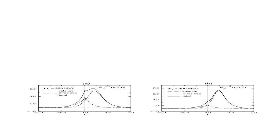
Figure 7: The $m_{\pi}$ dependence of $E_{M}^{u-d}(x,0,0)$.

Shown in Fig.6 and in Fig.7 are the CQSM predictions for $E_{M}^{(I=1)}(x,0,0)$ with several values of $m_{\pi}$. i.e. $m_{\pi}=0,200$, and $400\,\mbox{MeV}$. One clearly sees that the height of the peak around $x=0$, due to the deformed Dirac-sea quarks, decreases rapidly as $m_{\pi}$ increases. This supports our interpretation of this peak as the effects of pion clouds. On the other hand, one also observes that the magnitude of the valence quark contribution, peaked around $x\sim 1/3$, gradually increases as $m_{\pi}$ becomes large. This behavior of $E_{M}^{(I=1)}(x,0,0)$ turns out to cause a somewhat unexpected $m_{\pi}$ dependence of $G_{M,10}^{(I=1)}(0)$ and $G_{M,20}^{(I=1)}(0)$. As a function of $m_{\pi}$, the Dirac sea contribution to $G_{M,10}^{(I=1)}(0)$ decreases fast, whereas the valence quark contribution to it increases slowly, so that the total $G_{M,10}^{(I=1)}(0)$ becomes a decreasing function of $m_{\pi}$. On the other hand, owing to the approximate odd-function nature of the Dirac sea contribution to $xE_{M}^{(I=1)}(x,0,0)$ with respect to $x$, it hardly contributes to $G_{M,20}^{(I=0)}(0)$ independent of the pion mass, while the valence quark contribution to $xE_{M}^{(I=1)}(x,0,0)$ is an increasing function of $m_{\pi}$, thereby leading to the result that the net $G_{M,20}^{(I=0)}(0)$ is a increasing function of $m_{\pi}$.

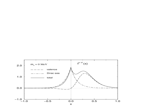
Figure 8: The prediction of the CQSM for $f^{u-d}(x,0,0)$ obtained with $M=400\,\mbox{MeV}$ and $m_{\pi}=0$.

Figure 9: The $m_{\pi}$ dependence of $f^{u-d}(x,0,0)$.

We can give still another support to the above-mentioned interpretation of the contribution of the Dirac-sea quarks. To see it, we first recall that the theoretical unpolarized distribution function $f^{u-d}(x)$ appearing in the decomposition

$$E_{M}^{u-d}(x,0,0)=f^{u-d}(x)+E^{u-d}(x,0,0),$$ (144)

also has a sizable peak around $x=0$ due to the deformed Dirac-sea quarks. As shown in Fig.8 and in Fig.9, this peak is again a rapidly decreasing function of $m_{\pi}$, supporting our interpretation of it as the effects of pion clouds. Here, we can say more. We point out that this small-$x$ behavior of $f^{u-d}(x)$ is just what is required by the famous NMC measurement NMC91 . To confirm it, first remember that the distribution $f^{u-d}(x)$ in the negative $x$ region should actually be interpreted as the distribution of antiquarks. To be explicit, it holds that

$$\bar{u}(x)-\bar{d}(x)=-f^{u-d}(-x)\ \ \ (x\geq 0).$$ (145)

The large and positive value of $f^{u-d}(x)$ in the negative $x$ region close to $x=0$ means that $\bar{u}(x)-\bar{d}(x)$ is negative, i.e. the dominance of the $\bar{d}$-quark over the $\bar{u}$-quark inside the proton, which has been established by the NMC measurement NMC91 .

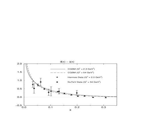
Figure 10: The prediction of the CQSM for $\bar{d}(x)-\bar{u}(x)$ evolved to $Q^{2}=2.3\,\mbox{GeV}^{2}$ and $Q^{2}=54\,\mbox{GeV}^{2}$ in comparison with the Hermes and NuTeV data at the corresponding energy scales HERMES98 ,E866 .

Shown in Fig.10 are the predictions of the CQSM for $\bar{d}(x)-\bar{u}(x)$ evolved to the high energy scales corresponding to the experimental observation Saga96 . (The theoretical predictions here were obtained with $M=400\,\mbox{MeV}$ and $m_{\pi}=100\,\mbox{MeV}$.) The model reproduces well the observed behavior of $\bar{d}(x)-\bar{u}(x)$, although the magnitude of the flavor asymmetry in smaller $x$ region seems to be slightly overestimated. It is a widely accepted fact that this flavor asymmetry of the sea quark distribution in the proton can physically be understood as the effects of pion cloud at least qualitatively HM91 –Wakamatsu92 . This then supports our interpretation of the effects of the deformed Dirac-sea quarks in $E_{M}^{(I=1)}(x,0,0)$ and $f^{u-d}(x)$ as the effects of pion clouds.

Table 1: The $m_{\pi}$ dependencies of $G_{M,20}^{(I=1)}(0)$, $G_{E,20}^{(I=1)}(0)$, and $B_{20}^{u-d}(0)$ in the CQSM with $M=400\,\mbox{MeV}$.

$m_{\pi}\,(\mbox{MeV})$	$G_{M,20}^{(I=1)}(0)$	$G_{E,20}^{(I=1)}(0)$	$B_{20}^{u-d}(0)$
0	0.361	0.228	0.133
100	0.392	0.276	0.116
200	0.452	0.327	0.125
300	0.519	0.350	0.169
400	0.579	0.354	0.225
500	0.640	0.347	0.293
600	0.716	0.328	0.388

We show in Table 1 the model predictions for $G_{M,20}^{(I=1)}(0),G_{E,20}^{(I=1)}(0)$, and $B_{20}^{u-d}(0)=G_{M,20}^{(I=1)}(0)-G_{E,20}^{(I=1)}(0)$ as functions of $m_{\pi}$. One sees that the value of $G_{M,20}^{(I=1)}(0)$ with $m_{\pi}=0$ is an order of $0.3\sim 0.4$. As already pointed out, it gradually increases as $m_{\pi}$ becomes large. This is also the case with $G_{E,20}^{(I=1)}(0)$. As a consequence, the isovector combination of the nucleon anomalous gravitomagnetic moment $B_{20}^{u-d}(0)$, which is obtained as a difference of the above two quantities, is also an increasing function of $m_{\pi}$, thereby having a tendency to come closer to the lattice prediction given in the heavy pion region. Still, the CQSM predictions $B_{20}^{u-d}(0)\simeq 0.3$ around $m_{\pi}=500\,\mbox{MeV}$ is a factor of two smaller than the corresponding lattice prediction $B_{20}^{u-d}(0)\simeq 0.6$. Now we summarize the reason why the CQSM gives fairly small prediction for $B_{20}^{u-d}(0)$. It is due to two types of cancellations. The first is the cancellation of the potentially large contribution of Dirac-sea quarks arising from the approximately antisymmetric behavior of the Dirac sea contribution to $xE_{M}^{(I=1)}(x,0,0)$ as well as $xf^{u-d}(x)$. The second is the cancellation between the total gravitomagnetic moment $G_{M,20}^{(I=1)}(0)$ and its canonical part $G_{E,20}^{(I=1)}(0)$. We are not sure whether the lattice simulation carried out in the heavy pion region with neglect of the so-called disconnected diagrams can efficiently take account of such effects of chiral dynamics as discussed above.

So far, we have investigated the pion mass dependence of the forward limit of the generalized form factors of the nucleon. Here, we investigate the momentum-transfer dependencies of some form factors of the nucleon. For the reason explained before, all the physical predictions given hereafter will be obtained with use of the mass parameter $M=400\,\mbox{MeV}$ and $m_{\pi}=100\,\mbox{MeV}$. We show in Fig.11, Fig.12, Fig.13, Fig.14 the predicted momentum-transfer dependencies of the generalized Sachs form factors, $G_{E,10}^{(I=0)}(t)$, $G_{E,20}^{(I=0)}(t)$, $G_{E,10}^{(I=1)}(t)$, $G_{E,20}^{(I=1)}(t)$, $G_{M,10}^{(I=0)}(t)$, $G_{M,20}^{(I=0)}(t)$, $G_{M,10}^{(I=1)}(t)$, and $G_{M,20}^{(I=1)}(t)$.

Figure 11: The predictions of the CQSM for the isoscalar generalized electric form factors $G^{(I=0)}_{E,10}(t)$ and $G^{(I=0)}_{E,20}(t)$.

Figure 12: The predictions of the CQSM for the isovector generalized electric form factors $G^{(I=1)}_{E,10}(t)$ and $G^{(I=1)}_{E,20}(t)$.

Figure 13: The predictions of the CQSM for the isoscalar generalized magnetic form factors $G^{(I=0)}_{M,10}(t)$ and $G^{(I=0)}_{M,20}(t)$.

Figure 14: The predictions of the CQSM for the isovector generalized magnetic form factors $G^{(I=1)}_{M,10}(t)$ and $G^{(I=1)}_{M,20}(t)$.

To get some feeling about the momentum-transfer dependencies of the predicted form factors, we shall compare them with the existing empirical data. At present, only the lowest moment of the GPDs, i.e. the standard electromagnetic form factors of the nucleon are experimentally known. Shown in Fig.15 are the predictions of the CQSM for the Dirac form factors of the proton and the neutron, in comparison with the empirical data Arnold86 together with the corresponding predictions at the LHPC lattice simulation LHPC04 ,LHPC05 . One observes that the $t$-dependence of the CQSM prediction for $F_{1}^{p}(t)$ is a little too stronger than the empirical one, while the t-dependence of the lattice predictions is too much weaker than the empirical one. A little too fast falloff of the CQSM predictions means that it slightly overestimates the electromagnetic size of the proton. On the contrary, the electromagnetic proton size predicted by the LHPC simulation is too small as compared with the empirically known size. As is well known, the Dirac form factor of the neutron is not well determined experimentally. Both of the CQSM prediction and the lattice QCD predictions are very small in magnitude in qualitatively consistent with the empirical information, although the former is slightly positive, while the latter is slightly negative.

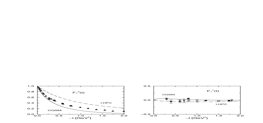
Figure 15: The prediction of the CQSM for the Dirac form factors of the proton and the neutron in comparison with the empirical data Arnold86 together with the LHPC lattice predictions. The LHPC lattice predictions are based on their dipole fits LHPC04 ,LHPC05 .

Fig.16 shows the predictions of the CQSM for the Pauli form factors of the proton and the neutron, in comparison with the empirical data together with the corresponding predictions of the LHPC lattice simulation. (Here, both of the CQSM predictions and the lattice QCD predictions are normalized to the observed anomalous magnetic moments of the proton and the neutron at the zero momentum transfer.) The solid curves represent the predictions of the CQSM, whereas the dashed curves show the corresponding lattice predictions. One can see that the predictions of the CQSM reproduce the empirical Pauli form factors fairly well. On the other hand, the lattice QCD predicts too slow falloff of the Pauli form factors, which means that the magnetic sizes of the nucleon are largely underestimated by the lattice QCD simulations. The underestimate of the nucleon electromagnetic sizes seems to be a general tendency of the lattice QCD simulations by the LHPC and QCDSF collaborations. It is not clear yet whether the origin of discrepancy can be traced back to the fact that these lattice simulations were carried out in the region with unrealistically heavy pion mass.

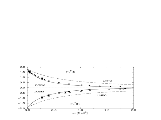
Figure 16: The predictions of the CQSM for the Pauli form factors of the proton and the neutron in comparison with the empirical data Arnold86 together with the LHPC lattice predictions based on the dipole fits LHPC04 ,LHPC05 .

Concerning the genuine generalized form factors with $n\geq 2$, we have no experimental information yet. Among them, of our particular interest is the generalized form factor $B_{20}^{u+d}(t)$ appearing in Ji’s angular momentum sum rule. We show in Fig.17 the prediction of the CQSM for $B_{20}^{u+d}(t)$ obtained with $M=400\,\mbox{MeV}$ and $m_{\pi}=100\,\mbox{MeV}$, in comparison with the corresponding predictions of the LHPC group. One sees that, for arbitrary value of $t$, $B_{20}^{u+d}(t)$ does not vanish in the CQSM, which is an indication of the fact that the shapes of the quark momentum and the total angular momentum distributions are not completely the same. Still, the magnitude of $B_{20}^{u+d}(t)$ turns out to be very small, which seems qualitatively compatible with the prediction of the LHPC group, although one should not forget about large uncertainties in the lattice simulation at the present level.

Figure 17: The predictions of the CQSM for the generalized form factor $B_{20}^{u+d}(t)$ of the nucleon, in comparison with the corresponding prediction of the lattice QCD by LHPC collaboration LHPC05 .

We are now ready to discuss what we can say about the spin contents of the nucleon from our investigation on the generalized form factors of the nucleon. The quantities of our interest are all obtained from the forward limit of the generalized form factors, which are defined as the second moments of the relevant GPDs :

$$\langle x\rangle^{u+d} = G_{E,20}^{(I=0)}(0),\ \ \ \ \ \langle x\rangle^{u-d}\ =\ G_{E,20}^{(I=1)}(0),$$ (146)

$$2\,J^{u+d} = G_{M,20}^{(I=0)}(0),\ \ \ \ \ 2\,J^{u-d}\ =\ G_{M,20}^{(I=1)}(0).$$ (147)

Summarized below are the predictions of the CQSM model for these quantities obtained with $M=400\,\mbox{MeV}$ and $m_{\pi}=100\,\mbox{MeV}$ :

$$\langle x\rangle^{u+d} = 1.00,\ \ \ \ \ \langle x\rangle^{u-d}=0.276,$$ (148)

$$2J^{u+d} = 1.00,\ \ \ \ \ 2J^{u-d}=0.406.$$ (149)

As pointed out before, these second moments of GPDs are generally scale dependent. Our viewpoint is that the predictions of the CQSM correspond to those at the low energy scale where the validity of the model is ensured. (This energy may typically be characterized by the Pauli-Villars mass $\Lambda_{1}\simeq 600\,\mbox{MeV}$.) We shall take account of the scale dependence of the above quantities by solving the QCD evolution equation at the next-to-leading order (NLO) with the predictions of the CQSM as the initial conditions FRS77 –ABY97 . For simplicity, let us assume that, at this low energy scale, there is no contribution of gluon fields as well as of the strange quarks, which dictates that

$$\langle x\rangle^{s}=0.0,\ \ \ 2\,J^{s}=0.0,\ \ \ \ \langle x\rangle^{g}=0.0,\ \ \ 2\,J^{g}=0.0.$$ (150)

The starting energy of the evolution is taken to be $Q_{ini}^{2}=0.30\,\mbox{GeV}^{2}\simeq(550\,\mbox{MeV})^{2}$, because it is favored from the previous successful application of the model to high energy deep-inelastic-scattering observables WK98 –Wakamatsu03b . Taking $N_{f}=3$ and $\Lambda_{QCD}=0.248\,\mbox{GeV}$, we find that, at $Q^{2}=4\,\mbox{GeV}^{2}$,

$$\langle x\rangle^{u+d+s} = 0.676,\ \ \ \langle x\rangle^{u-d}=0.171,\ \ \ \langle x\rangle^{g}=0.324,$$ (151)

$$2J^{u+d+s} = 0.676,\ \ \ 2J^{u-d}=0.257,\ \ \ \,2J^{g}=0.324.$$ (152)

One may notice that the values of $\langle x\rangle^{u+d+s}$ and $2\,J^{u+d+s}$ at $Q^{2}=4\,\mbox{GeV}^{2}$ precisely coincide. Actually, the equality of these two quantities holds at any energy scale. The reason is because these two quantities obey exactly the same evolution equation and because they are equal at the initial energy scale according to the CQSM JTH96 . (We emphasize that the latter is also the case for the LHPC and QCDSF lattice predictions at least approximately LHPC05 ,QCDSF04b .) In table 2, we compare these predictions of the CQSM with those of the lattice QCD and also with the empirical values for $\langle x\rangle^{u+d+s}$ and $\langle x\rangle^{u-d}$ obtained from the phenomenological PDF fits MRST2004 . As one sees, the total momentum fraction $\langle x\rangle^{u+d+s}$ carried by the quarks decreases rapidly as $Q^{2}$ increases. The evolved value $\langle x\rangle^{u+d}\simeq 0.68$ at $Q^{2}=4\,\mbox{GeV}^{2}$ is not extremely far from the lattice QCD prediction at the same normalization scale, although it is a little larger than the empirical value $\langle x\rangle^{u+d+s}_{empirical}\simeq 0.57$. This difference may be an indication of the fact that, even at the low energy scale around $Q^{2}\simeq 0.30\,\mbox{GeV}^{2}$, the gluons may carry some portion of the nucleon momentum. As far as the difference of the momentum fractions carried by the $u$-quark and the $d$-quark, the CQSM well reproduces the empirical value $\langle x\rangle^{u-d}_{empirical}\simeq 0.16$ at $Q^{2}=4\,\mbox{GeV}^{2}$, whereas the lattice QCD overestimates it a little.

Table 2: The predictions of the CQSM for ${\langle x\rangle}^{u+d}$, ${\langle x\rangle}^{u-d}$, $2\,J^{u+d}$, and $2\,J^{u-d}$ in comparison with the predictions of the lattice QCD simulations LHPC04 ,LHPC05 ,QCDSF04b ,QCDSF05 as well as with the empirical information MRST2004 .

	CQSM (model scale)	CQSM  ($Q^{2}=4\,\mbox{GeV}^{2})$	LHPC	QCDSF	empirical
${\langle x\rangle}^{u+d+s}$	1.000	0.676	0.61	0.59	0.57
${\langle x\rangle}^{u-d}$	0.276	0.171	0.269	0.24	0.157
$2\,J^{u+d+s}$	1.000	0.676	0.58	0.66	—
$2\,J^{u-d}$	0.406	0.257	0.93	0.82	—

Next we turn to the discussion of the total angular momenta $J^{u}$ and $J^{d}$ carried by the quark fields, on which we do not have any empirical information yet. One can see that, as far as the total angular momentum fraction $J^{u+d+s}$ carried by the quark fields, is concerned, the prediction of the CQSM is qualitatively consistent with that of the lattice QCD. However, a big discrepancy is observed for the difference $J^{u-d}$ of the angular momentum carried by the $u$-quark and the $d$-quark. The cause of this discrepancy can be traced back to that of the isovector gravitomagnetic moment of the nucleon $G_{M,20}^{(I=1)}(0)$, which we have already discussed. Fairly small prediction of the CQSM for $J^{u-d}$ also appears to be incompatible with the semi-theoretical (or semi-phenomenological) estimate carried out in GPV01 with partial use of the predictions of the CQSM. As we shall discuss below, however, their estimate for $J^{u}$ and $J^{d}$ shown in Table 4 and Table 5 of GPV01 should be taken with care. In fact, it was obtained based on the valence-like approximation, i.e. by neglecting the sizable Dirac sea contributions to $E^{u}(x,0,0)$ and $E^{d}(x,0,0)$. To be more concrete, they start with a simple guess for these distributions functions as

$$E^{u}(x,0,0) = \frac{1}{2}\,\kappa^{u}\,f^{u_{val}}(x),$$ (153)

$$E^{d}(x,0,0) = \ \ \kappa^{d}\,f^{d_{val}}(x),$$ (154)

with

$$\kappa^{u} = 2\,\kappa^{p}+\kappa^{u}=\ 1.673,$$ (155)

$$\kappa^{d} = \kappa^{p}+2\,\kappa^{u}=-\,2.033.$$ (156)

This parameterization trivially satisfies the 1st moment sum rule

$$\int_{-1}^{1}\,E^{q}(x,0,0)\,dx=\kappa^{q}.$$ (157)

On the other hand, by using the 2nd moment sum rule or Ji’s angular momentum sum rule, they obtain

$$J^{u} = \frac{1}{2}\,\left[\,{\langle x\rangle}^{u}+\kappa^{u}{\langle x\rangle}^{u_{val}}\right],$$ (158)

$$J^{d} = \frac{1}{2}\,\left[\,{\langle x\rangle}^{d}+\kappa^{d}{\langle x\rangle}^{d_{val}}\right],$$ (159)

where ${\langle x\rangle}^{q}$ is the momentum fraction carried by the quark of flavor $q$, while ${\langle x\rangle}^{q_{val}}$ is the corresponding contribution of the valence quark in the sense of parton model. Using the MRST98 parameterization for the unpolarized PDFs MRST98 , they could thus obtain at $Q^{2}\simeq 1\,\mbox{GeV}^{2}$

$${\langle x\rangle}^{u_{val}}\simeq 0.34,\ \ \ {\langle x\rangle}^{u}\simeq 0.40,\ \ \ 2\,J^{u}\simeq 0.69,$$ (160)

and

$${\langle x\rangle}^{d_{val}}\simeq 0.14,\ \ \ {\langle x\rangle}^{d}\simeq 0.22,\ \ \ 2\,J^{d}\simeq-0.07,$$ (161)

which appears to be qualitatively consistent with the lattice predictions. (Here, we have discarded the small contribution of the $s$-quark, for simplicity.) However, after this simple estimate for $J^{u}$ and $J^{d}$, they next try to take account of the sizable Dirac sea contribution to the distributions $E^{u}(x,0,0)$ and $E^{d}(x,0,0)$. As already shown in our exact model calculation, and as shown in Fig.8 of GPV01 , which is obtained based on the derivative-expansions-type approximation within the CQSM, the Dirac sea contribution to $E^{u-d}(x,0,0)$ has a narrow and positive peak around $x\simeq 0$. To simulate this narrowly peaked behavior of the Dirac-sea contribution, they propose to parameterize it by a $\delta$ function in $x$. The new and improved parameterization for $E^{u}(x,0,0)$ and $E^{d}(x,0,0)$ are then given as

$$E^{u}(x,0,0) = A^{u}\,f^{u_{val}}(x)+B^{u}\,\delta(x),$$ (162)

$$E^{d}(x,0,0) = A^{d}\,f^{d_{val}}(x)+B^{d}\,\delta(x).$$ (163)

From the 1st and 2nd sum rules for $E^{u}(x,0,0)$ and $E^{d}(x,0,0)$, they obtain

$$A^{u} = \frac{2\,J^{u}-{\langle x\rangle}^{u}}{{\langle x\rangle}^{u_{val}}},$$ (164)

$$A^{d} = \frac{2\,J^{d}-{\langle x\rangle}^{d}}{{\langle x\rangle}^{d_{val}}},$$ (165)

$$B^{u} = 2\,\left[\,\frac{1}{2}\,\kappa^{u}\ -\ \frac{2\,J^{u}-{\langle x\rangle}^{u}}{{\langle x\rangle}^{u_{val}}}\,\right],$$ (166)

$$B^{d} = \kappa^{d}-\frac{2J^{d}-{\langle x\rangle}^{d}}{{\langle x\rangle}^{d_{val}}}.$$ (167)

As pointed out in GPV01 , the total angular momentum carried by $u$- and $d$-quarks, $J^{u}$ and $J^{d}$, now enter as fit parameters in the parameterization of $E^{u}(x,0,0)$ and $E^{d}(x,0,0)$. If so, there is no compelling reason to believe that they are close to the estimate given in (158) and (159), obtained within the valence-type parameterization for $E^{u}(x,0,0)$ and $E^{d}(x,0,0)$. In fact, if one puts the estimate given in (160) and (161) into the above relations (165) $\sim$ (167), one obtains

$$A^{u}\simeq 0.853,\ \ \ A^{d}\simeq-2.071,\ \ \ B^{u}\simeq-0.033,\ \ \ B^{d}\simeq 0.038,$$ (168)

which dictates that the coefficients of the $\delta$ functions are small or nearly zero. This is only natural, since the used value of $J^{u}$ and $J^{d}$ are just estimated based on the valence-type parameterization for $E^{u}(x,0,0)$ and $E^{d}(x,0,0)$. Conversely speaking, the values of $J^{u}$ and $J^{d}$ quoted in Table 4 and table 5 of GPV01 need a revision, because they are incompatible with the existence of sharp peak of $E^{u-d}(x,0,0)$ with sizable positive magnitude around $x\simeq 0$ observed in Fig.8 of the same paper. The inseparable relation between the magnitude of $J^{u}-J^{d}$ and the sharp of $E^{u-d}(x,0,0)$ can be made more transparent by slightly modifying their schematic analysis. Instead of $E^{u-d}(x,0,0)$, we chose here to parameterize $E_{M}^{u-d}(x,0,0)\equiv H^{u-d}(x,0,0)+E^{u-d}(x,0,0)$ as

$$E_{M}^{u-d}(x,0,0)\ =\ c_{1}\,\left[\,f^{u_{val}}(x)-f^{d_{val}}(x)\,\right]\ +\ c_{2}\,\delta(x).$$ (169)

Here the $\delta$ function term is thought to simulate the sizable sharp peak of $E_{M}^{u-d}(x,0,0)$ predicted by the CQSM. Actually, it need not be a $\delta$ function. It can be an any function $g$ of $x$, as far as it satisfies the following two conditions :

• $g(x)$ is an even function of $x$ at least approximately,

• the integral of $g(x)$ over $x$ gives a (positive) number $c_{2}$.

Assuming that these conditions are satisfied (as is the case for the predictions of the CQSM), the 1st and the 2nd moment sum rule of $E^{u-d}_{M}(x,0,0)$ leads to the identities :

$$1+\kappa^{u}-\kappa^{d} = \int_{-1}^{1}E_{M}^{u-d}(x,0,0)\,dx\ =\ c_{1}\ +\ c_{2},$$ (170)

$$2\,(J^{u}-J^{d}) = \int_{-1}^{1}\,E_{M}^{u-d}(x,0,0)\,dx\ =\ c_{1}\,\left(\,\langle x\rangle^{u_{val}}-\langle x\rangle^{d_{val}}\,\right).$$ (171)

Combining these relations, we have

$$2\,(J^{u}-J^{d})=\frac{1+\kappa^{u}-\kappa^{d}}{1+r}\,\left(\,\langle x\rangle^{u_{val}}-\langle x\rangle^{d_{val}}\,\right).$$ (172)

Here we have introduced a parameter $r\equiv c_{2}/c_{1}$. This relation shows that, except for one parameter $r$, the difference of the total angular momenta, carried by the $u$- and $d$-quarks, $J^{u}-J^{d}$, is given by $\kappa^{u},\kappa^{d},\langle x\rangle^{u_{val}}$ and $\langle x\rangle^{d_{val}}$, which are all observables. What is the physical meaning of the parameter $r$, then ? To understand it, we first recall that the quantity $E_{M}^{u-d}(x,0,0)$ represents the distribution of the isovector magnetic moment of the nucleon in Feynman $x$-space not in ordinary coordinate space. The contribution of its valence-like distribution to the magnetic moment gives $c_{1}$, whereas that of its sea-like distribution gives $c_{2}$. The CQSM indicates that they are of approximately equal magnitude, i.e. $c_{1}\simeq c_{2}$, which means that $r\simeq 1$. On the other hand, roughly speaking, the lattice simulations carried out in the heavy pion region with neglect of the disconnected diagrams correspond to $r\simeq 0$.

Table 3: The value of $2\,(J^{u}-J^{d})$ as a functions of the ratio of the parameters $c_{2}$ and $c_{1}$ defined in (172).

$r\equiv c_{2}/c_{1}$	$2\,(J^{u}-J^{d})$
0	0.941
0.5	0.627
1	0.471

Table 3 show the values of $2(J^{u}-J^{d})$ obtained from (172) for several typical values of the ratio $r$. The quantity $\langle x\rangle^{u_{val}}-\langle x\rangle^{d_{val}}$ are actually scale dependent. For simplicity, here we have used the empirical value $\langle x\rangle^{u_{val}}-\langle x\rangle^{d_{val}}\simeq 0.2$ corresponding to $Q^{2}=1\,\mbox{GeV}^{2}$ quoted in GPV01 . One sees that the two cases, i.e. $r=0$ case and $r=1$ case, lead to a factor of two difference for $J^{u}-J^{d}$. What is indicated by this observation is an inseparable connection between the angular momentum carried by the quark fields in the nucleon and the magnetic moment of the nucleon, or more precisely the distribution of magnetic moments in Feynman $x$-space. As a matter of course, the relation between the quark angular momentum and the nucleon magnetic moment could be anticipated from more general ground of Ji’s angular momentum sum rule. However, an advantage of our explicit model analysis is that we can get more deep and concrete insight into the possible behavior of the relevant distribution $E^{u-d}(x,0,0)$, on which we have no experimental information yet.

Returning to the isoscalar (flavor-singlet) combination or the net quark contribution to the total angular momentum of the nucleon, $J^{u+d+s}$, we have pointed out that the prediction of the CQSM for it is not so far from that of the lattice QCD. However, both of LHPC and QCDSF collaborations also estimated the net orbital angular momentum carried by the quark fields, thereby being led to the conclusion that the total orbital angular momentum of the quarks is very small or consistent with zero. As pointed out in our recent paper, this conclusion contradicts not only the prediction of the CQSM but also the famous EMC observation. Although the possible reason of this discrepancy was already pointed out in that paper Wakamatsu05 , here we discuss it in more detail, especially by taking care of the scale dependencies of the relevant observables. The quark orbital angular momentum can be obtained by subtracting the intrinsic quark spin term from the total quark angular momentum $J^{u+d}$ as

$$L^{u+d}=J^{u+d}-\frac{1}{2}\,\Delta\Sigma^{u+d},$$ (173)

where $J^{u+d}$ is given by

$$J^{u+d}=\frac{1}{2}\,\left(\,\langle x\rangle^{u+d}+B_{20}^{u+d}(0)\right),$$ (174)

Using the results of the dipole fits for the generalized form factors, the LHPC collaboration obtain

$$\langle x\rangle^{u+d} = A_{20}^{u+d}(0)\ =\ 0.666\pm 0.009,$$ (175)

$$B_{20}^{u}(0) = 0.29\pm 0.04,\ \ \ B_{20}^{d}(0)\ =\ -\,0.38\pm 0.02,$$ (176)

$$\Delta\Sigma^{u} = 0.860\pm 0.069,\ \ \ \Delta\Sigma^{d}\ =\ -\,0.171\pm 0.043,$$ (177)

which in turn gives

$$L^{u}\ =\ -\,0.088\pm 0.019,\ \ \ L^{d}\ =\ 0.036\pm 0.013,$$ (178)

or

$$L^{u+d}\ =\ -\,0.052\pm 0.019.$$ (179)

On the other hand, the QCDSF collaboration obtain

$$\langle x\rangle^{u} = A_{20}^{u}(0)\ =\ 0.400\pm 0.022,\ \ \ \langle x\rangle^{d}\ =\ A_{20}^{d}(0)\ =\ 0.147\pm 0.011,$$ (180)

$$B_{20}^{u}(0) = 0.334\pm 0.113,\ \ \ B_{20}^{d}(0)\ =\ -\,0.232\pm 0.077,$$ (181)

$$\Delta\Sigma^{u} = 0.84\pm 0.02,\ \ \ \Delta\Sigma^{d}\ =\ -\,0.24\pm 0.02,$$ (182)

which gives

$$L^{u+d}\ =\ 0.03\pm 0.07.$$ (183)

As one sees, a common conclusion of the two groups is that the total orbital angular momentum of quarks is very small or consistent with zero.

Since these lattice predictions corresponds to the energy scale of $Q^{2}=4\,\mbox{GeV}^{2}$ in the $\overline{MS}$ scheme, we try to evolve the corresponding predictions of the CQSM to the same energy. To know the scale dependence of the total quark orbital angular momentum $L^{Q}$ with $Q$ denoting the sum of all quark flavors, we need to know the scale dependence of the total quark angular momentum $J^{Q}$ and that of the total quark longitudinal polarization $\Delta\Sigma^{Q}$. We recall again the fact that the angular momentum fractions carried by the quark and the gluon field, i.e. $J^{Q}$ and $J^{g}$, obey exactly the same evolution equation as the total momentum fractions carried by the quark and gluon fields $\langle x\rangle^{Q}$ and $\langle x\rangle^{g}$ JTH96 . The evolution equation of $\Delta\Sigma^{Q}$, which is coupled with the evolution of the gluon polarization, is also well known GRSV96 . As initial conditions of the evolution, we use the predictions of the CQSM (the flavor SU(2) version) :

$$2J^{u+d}=1.0,$$ (184)

supplemented with the assumption

$$\ \ 2\,J^{s}=0.0,\ \ \ \Delta\Sigma^{s}=0.0,\ \ \ \Delta g=0.0,$$ (185)

at $Q^{2}_{ini}=0.30\,\mbox{GeV}^{2}$. (There also exists the flavor SU(3) version of the CQSM Wakamatsu03a ,Wakamatsu03b . It predicts that $\Delta\Sigma^{s}$ is a negative quantity of the order of $(5\sim 10)\,\%$. However, the flavor singlet combination or the net quark contribution to the total quark longitudinal polarization $\Delta\Sigma^{Q}$ takes almost the same value in both version of the CQSM, so that the following discussion will receive no modification.)

Figure 18: The left panel shows the scale dependencies of the quark and gluon total angular momenta $J^{Q}$ and $J^{g}$ obtained by solving the evolution equation at the NLO with the predictions of the CQSM as initial conditions, while the right panel shows the scale dependence of $\Delta\Sigma^{Q}$ and $\Delta g$.

The left panel of Fig.18 shows the scale dependence of $J^{Q}$ obtained by solving the evolution equation at the NLO in the $\overline{MS}$ scheme. (Here we set $N_{c}=3$ and $\Lambda_{QCD}=0.248\,\mbox{GeV}$.) One observers that, especially at low energy scales, $J^{Q}$ is a rapidly decreasing function, while $J^{g}$ is a rapidly increasing function of $Q^{2}$. The right panel of Fig.18 shows the scale dependence of $\Delta\Sigma^{Q}$ and $\Delta g$ obtained by solving the NLO evolution equation in the same renormalization scheme GRSV96 . As one sees, $\Delta g$ is a rapidly-increasing function of $Q^{2}$. On the other hand, $\Delta\Sigma^{u+d+s}$ has a fairly weak scale dependence. Its scale dependence is restricted to the very low energy region below $Q^{2}\leq 0.6\,\mbox{GeV}^{2}$ and beyond that scale it changes very slowly. (We recall that, at the leading order (LO), $\Delta\Sigma^{Q}$ in the $\overline{MS}$ is exactly scale independent. One may also remember the fact that $\Delta\Sigma^{Q}$ in the chiral-invariant renormalization scheme is scale independent by definition LSS2000 –ABFS97 .) Now, combining the results for the scale dependencies of $J^{Q},J^{g},\Delta\Sigma^{Q}$, and $\Delta g$, one can predict the scale dependencies of $L^{Q}$ and $L^{g}$ at the NLO from

$$L^{Q} = J^{Q}-\frac{1}{2}\,\Delta\Sigma^{Q},$$ (186)

$$L^{g} = J^{g}-\Delta g.$$ (187)

Fig 19 shows the scale dependencies of quark and gluon orbital angular momenta obtained in this manner. One sees that the total quark orbital angular momentum is a rapidly decreasing functions of the energy scale, especially at the low energy scales. Since the longitudinal quark polarization is only weakly scale dependent, this feature comes from the scale dependence of the total quark angular momentum, which has the same scale dependence as the total quark momentum fraction. One also sees that the gluon orbital angular momentum is a decreasing function of the energy scale.

Figure 19: The scale dependencies of the quark and gluon orbital angular momenta $L^{Q}$ and $L^{g}$ at the NLO obtained with combined use of the predictions of the CQSM and the QCD evolution equations at the NLO.

For the sake of comparison with the lattice QCD predictions corresponding the the energy scale of $Q^{2}=4\,\mbox{GeV}^{2}$, we summarize in Table 4 the predictions of the CQSM for the nucleon spin contents at the same energy scale. One confirms that the total quark orbital angular momentum is a rapidly decreasing function of the energy scale and its value at $Q^{2}=4\,\mbox{GeV}^{2}$ is nearly half of that at the low energy model scale around $Q_{ini}^{2}=0.30\,\mbox{GeV}^{2}$. Nonetheless, it still bears a sizable amount of the total nucleon spin even at the scale $Q^{2}=4\,\mbox{GeV}^{2}$, in contrast to the lattice predictions. We point out that, after taking account of the scale dependence, the predictions for $J^{Q}$ are not so different between the CQSM and the lattice QCD. What is remarkably different is the predictions of the two theories for the net longitudinal quark polarization or the contribution of intrinsic quark spin. It is clear that the lattice QCD simulations by the LHPC and the QCDSF collaborations for $\Delta\Sigma^{Q}$ considerably overestimate the empirically known value of $\Delta\Sigma^{Q}$, which is known to be quite small as

$$\Delta\Sigma^{Q}_{empirical}=(0.2\sim 0.35),$$ (188)

while the prediction of the CQSM is qualitatively consistent with this empirical information. A plausible reason why the lattice simulations by the LHPC and the QCDSF collaboration predicts fairly large $\Delta\Sigma^{Q}$ around $0.6$ was pointed out in WT05 . In that paper, we investigated the pion mass dependence of $\Delta\Sigma^{Q}$ within the framework of the CQSM and found that it is very sensitive to the variation of $m_{\pi}$, especially in the region close to the chiral limit $m_{\pi}=0$. (The magnitude of $\Delta\Sigma^{Q}$ decreases rapidly as $m_{\pi}$ approaches $0$.) This indicates that the lattice estimates carried out in the heavy pion region around $m_{\pi}=(700\sim 900)\,\mbox{MeV}$ may not give reliable prediction for the particular observable $\Delta\Sigma^{Q}$. As a consequence, their conclusion that the orbital angular momentum carried by the quark fields in the nucleon is negligible, must also be taken with care. It may be justified in the heavy pion world, but whether it is also the case in our chiral world is a different question, which should be answered by the lattice QCD studies in the future.

Also noteworthy is the fact that the large values of $\Delta\Sigma^{u+d}$ obtained by the LHPC and QCDSF lattice collaborations seem to contradict the results of earlier lattice QCD studies MDLMM00 –DLL95 , which predict fairly small $\Delta\Sigma^{Q}$ around $(0.2\sim 0.3)$. Among them, Mathur et. al. MDLMM00 also estimated the total quark angular momentum $J^{Q}$ from the quark energy-momentum tensor form factors on the lattice with the quenched approximation, and deduced that the quark orbital angular momentum carries about $34\,\%$ of the total proton spin, which is compatible or even dominant over the contribution of intrinsic quark spin around $26\,\%$ obtained by their simulation.

Table 4: The predictions of the CQSM for the spin contents of the nucleon in comparison with the corresponding predictions of the LHPC and QCDSF lattice QCD simulations LHPC05 ,QCDSF04b .

	CQSM (model scale)	CQSM  ($Q^{2}=4\,\mbox{GeV}^{2})$	LHPC	QCDSF
$2\,J^{u+d+s}$	1.000	0.676	0.56	0.66
$\Delta\Sigma^{u+d+s}$	0.350	0.318	0.69	0.60
$2\,L^{u+d+s}$	0.650	0.358	-0.11	0.06

So far, we have given several interesting theoretical predictions on the basis of an effective theory of QCD, i.e. the CQSM. Although we believe that the reliability of these predictions is guaranteed by the phenomenological success of the CQSM achieved in the nucleon structure function physics, it would be nicer if one can extract some predictions, which do not depend on a specific model of the nucleon. It is in fact possible, if one accepts the following two theoretical postulates. They are

• Ji’s angular momentum sum rule  :  $J^{Q}=\frac{1}{2}\,[\langle x\rangle^{Q}+B_{20}^{Q}(0)]$ ,

• absence of the net quark contribution to the anomalous gravitomagnetic moment of the nucleon  :  $B_{20}^{Q}(0)=0$ .

It is reasonable to accept the first postulate. Otherwise, we would lose a only clue to experimentally access the quark angular momentum in the nucleon. What is crucial in the following argument is therefore the second postulate. As already mentioned, the identity $B_{20}^{Q}(0)=0$, that holds within the CQSM, just follows from the total momentum and the total angular momentum sum rules, both of which are saturated by the quark fields alone in this effective quark theory. It can therefore be an artifact of the model. However, an interesting observation is that the smallness of $B_{20}^{Q}(0)$ is also the predictions of the LHPC and the QCDSF lattice QCD simulations, which take account of full quark-gluon dynamics. Naturally, one should not forget about large uncertainties in the lattice simulations at the present stage. One should also worry about the $m_{\pi}$-dependence of $B_{20}^{Q}(0)$, although we conjecture from our analyses in the CQSM a weak $m_{\pi}$-dependence of this quantity.

Here, we shall proceed by assuming that $B_{20}^{Q}(0)$ vanishes exactly or at least very small. As already pointed out, the identity $B_{20}^{Q}(0)$ leads to remarkable relations, i.e. the proportionality of the total momentum and total angular momentum carried by the quark fields and also by the gluon fields as

$$J^{Q}=\frac{1}{2}\,\langle x\rangle^{Q},\ \ \ J^{g}=\frac{1}{2}\,\langle x\rangle^{g}.$$ (189)

An important fact here is that the quark and gluon momentum fractions, i.e. $\langle x\rangle^{Q}$ and $\langle x\rangle^{g}$ are empirically known with fairly good precision. For instance, the two popular PDF fits, i.e. MRST2004 and CTEQ5, give almost the same answer for $\langle x\rangle^{Q}$ and $\langle x\rangle^{g}$ at least within the energy range $Q^{2}\leq 10\,\mbox{GeV}^{2}$. There also exist phenomenological fits for the longitudinally polarized PDFs, which contains the information on $\Delta\Sigma^{Q}$ and $\Delta g$, although with larger uncertainties compared with the unpolarized case. These phenomenological PDFs can therefore be used for estimating the orbital angular momenta carries by the quark fields and the gluon fields through the relations :

$$L^{Q} = J^{Q}-\frac{1}{2}\,\Delta\Sigma^{Q},$$ (190)

$$L^{g} = J^{g}-\Delta g.$$ (191)

The values of $L^{Q}$ and $L^{g}$ at $Q^{2}=4\,\mbox{GeV}^{2}$ estimated in this way are shown in Table.5. Here, we use MRST2004 PDF fit to estimate $J^{Q}$ and $J^{g}$ MRST2004 . On the other hand, $\Delta\Sigma^{Q}$ and $\Delta g$ are estimated by using three independent PDF fits, i.e. LSS2005, DNS2005, and GRSV2000 LSS2005 ,DNS2005 ,GRSV2000 . Here, all of the three independent fits we are using correspond to the $\overline{\rm MS}$ regularization scheme. As one sees, there are sizable uncertainties for the phenomenological values of $\Delta\Sigma^{Q}$ and $\Delta g$. Still, a common conclusion obtained from all these PDF fits is a very important role of the quark orbital angular momentum. The table 5 shows, at the least, that the magnitude of the quark orbital angular momentum is comparable with that of the intrinsic quark spin even at the scale of $Q^{2}=4\,\mbox{GeV}^{2}$. Since the quark orbital angular momentum is a rapidly decreasing function of the energy scale, while the scale dependence of $\Delta\Sigma^{Q}$ is very weak, this means that the former is dominant over the latter at the scale below $Q^{2}\simeq 1\,\mbox{GeV}^{2}$ where any low energy models are supposed to hold. Naturally, the whole argument here is crucially dependent on one theoretical postulate that $B_{20}^{Q}(0)\simeq 0$. Although it is supported by both of the LHPC and QCDSF lattice simulations, efforts to improve the accuracy of the lattice prediction should be continued, in consideration of its extremely important role in determining the quark-gluon contents of the nucleon spin. Also highly desirable is an analytical proof of it within the framework of (nonperturbative) QCD.

Table 5: The model independent predictions of the spin contents of the nucleon at $Q^{2}=4\,\mbox{GeV}^{2}$, based only upon one theoretical postulate $B_{20}^{Q}(0)=0$. Here, all of the three independent fits for the longitudinally polarized PDFs correspond to the $\overline{\rm MS}$ scheme.

MRST2004		LSS2005		MRST2004 + LSS2005
$J^{Q}$	$J^{g}$	$\Delta\Sigma$	$\Delta g$	$L^{Q}$	$L^{g}$
0.289	0.211	0.198	0.368	0.190	-0.157
MRST2004		DNS2005		MRST2004 + DNS2005
$J^{Q}$	$J^{g}$	$\Delta\Sigma$	$\Delta g$	$L^{Q}$	$L^{g}$
0.289	0.211	0.313	0.477	0.133	-0.266
MRST2004		GRSV2000		MRST2004 + GRSV2000
$J^{Q}$	$J^{g}$	$\Delta\Sigma$	$\Delta g$	$L^{Q}$	$L^{g}$
0.289	0.211	0.137	0.623	0.221	-0.412

V Concluding remarks

In this paper, we have investigated the generalized form factors of the nucleon, which will be extracted through near-future measurements of the generalized parton distribution functions, within the framework of the CQSM. A particular emphasis is put on the pion mass dependence as well as the scale dependence of the model predictions, which we compare with the corresponding predictions of the lattice QCD by the LHPC and the QCDSF collaborations carried out in the heavy pion regime around $m_{\pi}\simeq(700\sim 900)\,\mbox{MeV}$. The generalized form factors contain the ordinary electromagnetic form factors of the nucleon such as the Dirac and Pauli form factors of the proton and the neutron. We have shown that the CQSM with good chiral symmetry reproduces well the general behaviors of the observed electromagnetic form factors, while the lattice simulations by the above two groups have a tendency to underestimate the electromagnetic sizes of the nucleon. Undoubtedly, this cannot be unrelated to the fact that the above two lattice simulations were performed with unrealistically heavy pion mass.

We have also tried to figure out the underlying spin contents of the nucleon through the analysis of the gravitoelectric and gravitomagnetic form factors of the nucleon, by taking care of the pion mass despondencies as well as of the scale dependencies of the relevant quantities. After taking account of the scale dependencies by means of the QCD evolution equations at the NLO in the $\overline{MS}$ scheme, the CQSM predicts, at $Q^{2}=4\,\mbox{GeV}^{2}$, that $2\,J^{Q}\simeq 0.68,\Delta\Sigma^{Q}\simeq 0.32$, and $2\,L^{Q}\simeq 0.36$, which means that the quark orbital angular momentum carries sizable amount of total nucleon spin even at such a relatively high energy scale. It contradicts the conclusion of the LHPC and QCDSF collaborations indicating that the total orbital angular momentum of quarks is very small or consistent with zero. It should be recognized, however, that the prediction of the CQSM for the total quark angular momentum is not extremely far from the corresponding lattice prediction $2\,J^{Q}\simeq 0.6$ at the same renormalization scale. The cause of discrepancy can therefore be traced back to the LHPC and QCDSF lattice QCD predictions for the quark spin fraction $\Delta\Sigma^{Q}$ around 0.6, which contradicts not only the prediction of the CQSM but also the EMC observation. As was shown in our recent paper Wakamatsu05 , $\Delta\Sigma^{Q}$ is such a quantity that is extremely sensitive to the variation of the pion mass, especially in the region close to the chiral limit. More serious lattice QCD studies on the $m_{\pi}$-dependence of $\Delta\Sigma^{Q}$ is highly desirable.

Worthy of special mention is the fact that, once we accept a theoretical postulate $B_{20}^{Q}(0)=0$, i.e, the absence of the net quark contribution to the anomalous gravitomagnetic moment of the nucleon, which is supported by both of the LHPC and QCDSF lattice simulations, we are necessarily led to a surprisingly simple relations, $J^{Q}=\frac{1}{2}\,\langle x\rangle^{Q}$ and $J^{g}=\frac{1}{2}\,\langle x\rangle^{g}$, i.e. the proportionality of the linear and angular momentum fractions carried by the quarks and the gluons. Using these relations, together with the existing empirical information for the unpolarized and the longitudinally polarized PDFs, we can give model-independent predictions for the quark and gluon contents of the nucleon spin. For instance, with combined use of the MRST2004 fit MRST2004 and the DNS2005 fit DNS2005 , we obtain $2\,J^{Q}\simeq 0.58$, $\Delta\Sigma^{Q}\simeq 0.31$, and $2\,L^{Q}\simeq 0.27$ at $Q^{2}=4\,\mbox{GeV}^{2}$. Since $L^{Q}$ (as well as $J^{Q}$) is a rapidly decreasing function of the energy scale, while the scale dependence of $\Delta\Sigma^{Q}$ is very weak, we must conclude that the former is even more dominant over the latter at the scale below $Q^{2}\simeq 1\,\mbox{GeV}^{2}$ where any low energy models are supposed to hold.

The situation is a little more complicated in the flavor-nonsinglet (or isovector) channel, because $B_{20}^{u-d}(0)\equiv G_{M,20}^{(I=1)}(0)-G_{E,20}^{(I=1)}(0)=2\,J^{u-d}-\langle x\rangle^{u-d}\neq 0$, and also because the CQSM and the lattice QCD give fairly different predictions for $G_{M,20}^{(I=1)}(0)$. As compared with the lattice prediction for $G_{M,20}^{(I=1)}(0)$ around $0.8$, the predictions of the CQSM turns out to be around $0.4$. We have argued that the relatively small value of $G_{M,20}^{(I=1)}(0)$ obtained in the CQSM is intimately connected with the small $x$ enhancement of the generalized parton distribution $E_{M}^{(I=1)}(x,0,0)$, which is dominated by the clouds of pionic $q\bar{q}$ excitation around $x\simeq 0$. (We recall that the 2nd moment of $E_{M}^{(I=1)}(x,0,0)$ gives $G_{M,20}^{(I=1)}(0)$.) Unfortunately, such a $x$-dependent distribution as $E_{M}^{(I=1)}(x,0,0)$ cannot be accessed within the framework of lattice QCD. Still, the predicted small $x$ behavior of $E_{M}^{u-d}(x,0,0)\equiv E_{M}^{(I=1)}(x,0,0)$ as well as of $f^{u-d}(x)$ indicates again the importance of chiral dynamics in the nucleon structure function physics, which has not been fully accounted for in the lattice QCD simulation at the present level.

Appendix A proof of the momentum sum rule

Here we closely follow the proof of the momentum sum rule given in DPPPW96 , by taking into account a necessary modification in the case of $m_{\pi}\neq 0$. The starting point is the following expression for the soliton mass (or the static soliton energy) :

$$M_{N}\ =\ N_{c}\,\mbox{Sp}[\,\theta(E_{0}-H+i\varepsilon)\,H\,]\ -\ (H\rightarrow H_{0})\ +\ E_{M},$$ (192)

with

$$E_{M}[F(r)]\ =\ -\,f_{\pi}^{2}\,m_{\pi}^{2}\,\int\,[\cos F(r)-1]\,d^{3}x.$$ (193)

The soliton mass must be stationary with respect to an arbitrary variation of the chiral field $U$ or equivalently the soliton profile $F(r)$, which lead to a saddle point equation :

$$\mbox{Sp}\,[\theta(E_{0}-H+i\varepsilon)\,\delta H]\ +\ \delta E_{m}\ =\ 0.$$ (194)

Here we consider a particular (dilatational) variation of chiral field

$$U(x)\longrightarrow U((1+\xi)x).$$ (195)

For infinitesimal $\xi$, we have

$$\delta U\equiv U((1+\xi)x)-U(x)\ \simeq\ \xi\,x^{k}\,\partial_{k}U(x),$$ (196)

so that

$$\delta H = M\,\gamma^{0}\,\xi\,x^{k}\,\partial_{k}U^{\gamma_{5}}\ =\ \xi\,[x^{k}\partial_{k},M\gamma^{0}U^{\gamma_{5}}]\ =\ \xi\,([x^{k}\partial_{k},H]-i\gamma^{0}\gamma^{k}\partial_{k}).$$ (197)

Noting the identity

$$\mbox{Sp}(\theta(E_{0}-H+i\varepsilon)[x^{k}\partial_{k},H])\ =\ \mbox{Sp}([H,\theta(E_{0}-H+i\varepsilon)]x^{k}\partial_{k})\ =\ 0,$$ (198)

we therefore obtain a key identity

$$\xi\,\mbox{Sp}[\theta(E_{0}-H+i\varepsilon)(-i)\gamma^{0}\gamma^{k}\partial_{k}]=-\,\delta E_{M}.$$ (199)

Now, by using (193) together with the relations,

$$\delta F(r) = \xi\,r\,F^{\prime}(r),$$ (200)

$$\delta\cos F(r) = -\,\sin F(r)\,\delta F=-\,\xi\,r\,\sin F(r)\,F^{\prime}(r),$$ (201)

we get

$$\delta E_{M} = \xi\cdot 4\pi\,f_{\pi}^{2}\,m_{\pi}^{2}\,\int_{0}^{\infty}\,dr\,r^{3}\,\sin F(r)\,F^{\prime}(r)$$ (202)

$$= -\,\xi\cdot 4\pi\,f_{\pi}^{2}\,m_{\pi}^{2}\,\int_{0}^{\infty}\,dr\,r^{3}\,\frac{d}{dr}\cos F(r).$$ (203)

Here, taking account of the boundary condition

$$F(0)=\pi,\ \ \ F(\infty)=0,$$ (204)

we can manipulate as

$$\int_{0}^{\infty}\,dr\,r^{3}\,\frac{d}{dr}\cos F(r) = \int_{0}^{\infty}\,dr\,r^{3}\,\frac{d}{dr}\,(\cos F(r)-1)$$ (205)

$$= r^{3}\,(\cos F(r)-1)|_{0}^{\infty}\ -\ 3\,\int_{0}^{\infty}\,dr\,r^{2}\,(\cos F(r)-1)$$ (206)

$$= -\,3\,\int_{0}^{\infty}\,dr\,r^{2}\,(\cos F(r)-1).$$ (207)

We thus find an important relation :

$$\delta E_{M}\ =\ -\,3\,\xi\,E_{M}.$$ (208)

Putting this relation into (199), we have

$$\xi\,\mbox{Sp}(\theta(E_{0}-H+i\varepsilon)\mbox{\boldmath$\alpha$}\cdot\mbox{\boldmath$p$})=3\,\xi\,E_{M},$$ (209)

or

$$\frac{1}{3}\,\mbox{Sp}(\theta(E_{0}-H+i\varepsilon)\mbox{\boldmath$\alpha$}\cdot\mbox{\boldmath$p$})=E_{M}.$$ (210)

If we evaluate the trace sum above by using the eigenstates of the static Dirac Hamiltonian $H$ as a complete set of basis, (210) can also be written as

$$\sum_{n\leq 0}\,\langle n|\,\frac{1}{3}\,\mbox{\boldmath$\alpha$}\cdot\mbox{\boldmath$p$}\,|n\rangle=E_{M},$$ (211)

which is the relation quoted in (84). We point out that our result has a correct chiral limit, since $E_{M}\rightarrow 0$ as $m_{\pi}\rightarrow 0$ and therefore

$$\lim_{m_{\pi}\rightarrow 0}\,\sum_{n\leq 0}\,\langle n|\,\frac{1}{3}\,\mbox{\boldmath$\alpha$}\cdot\mbox{\boldmath$p$}\,|n\rangle\ =\ 0,$$ (212)

in conformity with the proof given in ref.DPPPW96 .

References

- (1) EMC Collaboration : J. Aschman et al. Phys. Lett., B206:364, 1988.
- (2) EMC Collaboration : J. Aschman et al. Nucl. Phys., B328:1, 1989.
- (3) D. Mueller, D. Robaschik, B. Geyer, F.M. Dittes, and J. Horejsi, Fortsch. Phys., 42:101, 1994.
- (4) F.M. Dittes, D. Mueller, D. Robaschik, B. Geyer, and J. Horejsi, Phys. Lett., B209:325, 1988.
- (5) X. Ji. J. Phys., G24:1181, 1998.
- (6) K. Goeke, M.V. Polyakov, and M. Vanderhaeghen Prog. Part. Nucl. Phys., 47:401, 2001.
- (7) M. Diehl. Phys. Rep., 388:41, 2003.
- (8) A.V. Belitsky and A.V. Radyushkin. Phys. Rep., 418:1, 2005.
- (9) X. Ji. Phys. Rev. Lett., 78:610, 1997.
- (10) P. Hoodbhoy, X. Ji, and W. Lu. Phys. Rev., D59:014013, 1999.
- (11) X. Ji, J. Tang, and P. Hoodbhoy. Phys. Rev. Lett., 76:740, 1996.
- (12) M. Burkardt. Phys. Rev., D62:071503, 2000.
- (13) M. Burkardt. Int. J. Mod. Phys., A18:173, 2003.
- (14) J.P. Ralston and B. Pire. Phys. Rev., D66:111501, 2002.
- (15) M. Diehl, Th. Feldmann, R. Jacob and P. Kroll. Eur. Phys. J., C39:1, 2005.
- (16) M. Diehl. hep-ph/0510221.
- (17) D. Dolgov et al. Phys. Rev., D66:034506, 2002.
- (18) Ph. Hägler, J.W Negele, D.B. Renner, W. Schroers, Th. Lippert and K. Schilling. Phys. Rev. Lett., 93:112001, 2004.
- (19) Ph. Hägler, J.W Negele, D.B. Renner, W. Schroers, Th. Lippert and K. Schilling. Eur. Phys. J., A24:29, 2005.
- (20) QCDSF Collaboration : M. Göckeler, Ph. Hägler, R. Horsley, D. Pleiter, P.E.L. Rakow, A. Schäfer, G. Schierholz, and J.M. Zanotti. Few-Body Systems, 36:111, 2005.
- (21) M. Göckeler, R. Horsley, D. Pleiter, P.E.L. Rakow, A. Schäfer, G. Schierholz, and W. Schroers. Phys. Rev. Lett., 92:042002, 2004.
- (22) M. Göckeler, T.R. Hemmert, R. Horsley, D. Pleiter, P.E.L. Rakow, A. Schäfer, G. Schierholz, and W. Schroers. Nucl. Phys. (Proc. Suppl.), 128:203, 2004.
- (23) D.I. Diakonov, V.Yu. Petrov, and P.V. Pobylitsa. Nucl. Phys., B306:809, 1988.
- (24) M. Wakamatsu and H. Yoshiki. Nucl. Phys., A524:561, 1991.
- (25) S. Kahana and G. Ripka. Nucl. Phys., A429:462, 1984.
- (26) S. Kahana, G. Ripka, and V. Soni. Nucl. Phys., A415:351, 1984.
- (27) T. Kubota, M. Wakamatsu, and T. Watabe. Phys. Rev., D60:014016, 1999.
- (28) J. Ossmann, M.V. Polyakov, P. Schweitzer, D. Urbano, and K. Goeke. Phys. Rev., D71:034011, 2005.
- (29) M. Wakamatsu and H. Tsujimoto. Phys. Rev., D71:074001, 2005.
- (30) V.Yu. Petrov, P.V. Pobylitsa, M.V. Polyakov, I. Böring, K. Goeke and C. Weiss. Phys. Rev., D57:4325, 1998.
- (31) D.I. Diakonov, V.Yu. Petrov, P.V. Pobylitsa, M.V. Polyakov, and C. Weiss. Nucl. Phys., B480:341, 1996.
- (32) S.J. Brodsky, D.S. Hwang, B.-Q. Ma, and I. Schmidt. Nucl. Phys., B593:311, 2001.
- (33) M. Wakamatsu. Prog. Theor. Phys. Suppl., 109:115, 1992.
- (34) Chr.V. Christov, A. Blotz, H.-C. Kim, P. Pobylitsa, T. Watabe Th.Meissner, E.Ruiz-Arriola, and K. Goeke. Prog. Part. Nucl. Phys., 37:91, 1996.
- (35) R. Alkofer, H. Reinhardt, and H. Weigel. Phys. Rep., 265:139, 1996.
- (36) H. Weigel, L. Gamberg, and H. Reinhardt. Mod. Phys. Lett., A11:3021, 1996.
- (37) L. Gamberg, H. Reinhardt, and H. Weigel. Phys. Rev., D58:054014, 1998.
- (38) D.I. Diakonov, V.Yu. Petrov, P.V. Pobylitsa, M.V. Polyakov, and C. Weiss. Phys. Rev., D56:4069, 1997.
- (39) M. Wakamatsu and T. Kubota. Phys. Rev., D57:5755, 1998.
- (40) M. Wakamatsu and T. Kubota. Phys. Rev., D60:034020, 1999.
- (41) M. Wakamatsu. Phys. Rev., D67:034005, 2003.
- (42) M. Wakamatsu. Phys. Rev., D67:034006, 2003.
- (43) P.V. Pobylitsa, M.V. Polyakov, K. Goeke, T. Watabe, and C. Weiss. Phys. Rev., D59:034024, 1999.
- (44) M. Wakamatsu. Phys. Rev., D46:3762, 1992.
- (45) Chr.V. Christov, A.Z. Górski, K. Goeke, and P.V. Pobylitsa. Phys. Rev., A592:513, 1995.
- (46) M. Wakamatsu. Phys. Rev., D72:074006, 2005.
- (47) O.V. Teryaev. hep-ph/9904376, 1999.
- (48) O.V. Teryaev. hep-ph/9803403, 1998.
- (49) O.V. Teryaev. Czech. J. Phys., 53:47, 2003.
- (50) M. Wakamatsu and T. Watabe. Phys. Lett., B312:184, 1993.
- (51) Chr.V. Christov, A. Blotz, K. Goeke, P. Pobylitsa, V.Yu. Petrov, M. Wakamatsu, and T. Watabe. Phys. Lett., B325:467, 1994.
- (52) M. Wakamatsu. Prog. Theor. Phys., 95:143, 1996.
- (53) NMC Collaboration : P. Amaudruz et al. Phys. Rev. Lett., 66:2712, 1991.
- (54) M. Miyama and S. Kumano. Compt. Phys. Commun., 94:185, 1996.
- (55) E.M. Henley and G.A. Miller. Phys. Lett., B251:453, 1991.
- (56) S. Kumano and J.T. Londergan. Phys. Rev., D43:59, 1991.. AIP Conf. Proc. 223, 1991.
- (57) HEREMES Collaboration : K. Ackerstaff. Phys. Rev. Lett., 81:5519, 1998.
- (58) E866 Collaboration : E.A. Hawker et al. Phys. Rev. Lett., 80:3715, 1998.
- (59) R. Arnold et al. Phys. Rev. Lett., 57:174, 1986.
- (60) E.G. Floratos, D.A.. Ross, and C.T. Sachrajda. Nucl. Phys., B129:66, 1977, and Erratum, B139:545, 1978.
- (61) C. Lopéz and F.J. Ynduráin. Nucl. Phys., B183:157, 1981.
- (62) K. Adel, F. Barreiro, and F.J. Ynduráin. Nucl. Phys., B495:221, 1997.
- (63) A.D. Martin, R.G. Roberts, W.J. Stirling, and R.S. Thorne. Eur. Phys. J., C4:463, 1998.
- (64) A.D. Martin, W.J. Stirling, and R.S. Thorne. hep-ph/0603143, 2006.
- (65) L.H. Lai, J. Huston, S. Kuhlmann, J. Morfin, F. Olness, J.F. Owen, J. Pumplin, and W.K. Tung. Eur. Phys. J., C12:375, 2000.
- (66) M. Glück. E. Reya, and M. Strattmann, and W. Vogelsang. Phys. Rev., D63:094005, 2001.
- (67) E. Leader. A.V. Sidorov, and D.B. Stamenov. Phys. Rev., D73:034023, 2006.
- (68) D.de Florian, G.A. Navarro, and R. Sassot. Phys. Rev., D71:094018, 2005.
- (69) M. Glück. E. Reya, M. Strattmann, and W. Vogelsang. Phys. Rev., D53:4775, 1996.
- (70) E. Leader. A.V. Sidorov, and D.B. Stamenov. Phys. Lett., B488:283, 2000.
- (71) H.-Y. Cheng. Phys. Lett., B427:371, 1998.
- (72) R.D. Ball. S. Forte, and G. Ridolfi. Phys. Lett., B378:255, 1996.
- (73) G. Altarelli, R.D. Ball. S. Forte, and G. Ridolfi. Nucl. Phys., B496:337, 1997.
- (74) N. Mathur, S.J. Dong. K.F. Liu, L. Mankiewicz, and N.C. Mukhopadhyay. Phys. Rev., D62:114504, 2000.
- (75) M. Fukugita. Y. Kuramashi, M. Okawa, and A. Ukawa. Phys. Phys. Lett., 75:2092, 1995.
- (76) S.J. Dong. J.-F.Lagaë, and K.F. Liu. Phys. Phys. Lett., 75:2096, 1995.