Unification and fermion mass relations in low string scale D-brane models

Abstract

In this talk, gauge coupling evolution is analyzed in D-brane inspired models with two Higgs doublets and a $U(3)\times U(2)\times U(1)^{N}$ gauge symmetry. In particular, we focus on D-brane configurations with two or three abelian factors. We find that the correct hypercharge assignment of the Standard Model particles is reproduced for six viable models distinguished by different brane configurations. We also investigate the bottom tau quark mass relation and find that the correct low energy $m_{b}/m_{\tau}$ ratio is obtained for equal $b-\tau$ Yukawa couplings at a string scale around $10^{3}$ TeV.

1 Introduction

Low scale unification of gauge and gravitational interactions  [1, 2, 3], appears to be a promising framework for solving the hierarchy problem. In this context, the weakness of the gravitational force in long distances is attributed to the existence of extra dimensions at the Fermi scale. A realization of this scenario can occur in type I string theory [4] where gauge interactions are mediated by open strings with their ends attached on some D-brane stack, while gravity is mediated by closed strings that propagate in the whole 10 dimensional space.

In the context of Type I string theory using appropriate collections of parallel [5, 6] or intersecting [7, 8] D-branes, there has been considerable work in trying to derive the Standard Model theory or its Grand Unified extensions [9, 10, 11, 12, 13, 14, 15, 16, 17, 18, 19]. Some of these low energy models revealed rather interesting features: (i) The correct value of the weak mixing angle is obtained for a string scale of the order of a few TeV (ii) baryon and lepton numbers are conserved due to the existence of exact global symmetries which are remnants of additional anomalous $U(1)$ factors broken by the Green-Schwarz mechanism (iii) supersymmetry is not necessary to solve the hierarchy problem.

However, its rivals, supersymmetric Grand Unified theories (where the unification of gauge couplings occurs at the order of $10^{16}$ GeV), and their heterotic string realizations (with even higher unification scale), exhibit also a number of additional interesting features. Apart from the natural gauge coupling unification these features include fermion mass [20, 21] relations and in particular the bottom tau-unification, i.e. the equality of the corresponding Yukawa couplings at the unification scale, which reproduces the correct mass relation at low energies.

Full gauge coupling unification does not occur in low string scale models, however, this should not be considered as a drawback since the various gauge group factors are associated with different stacks of branes and therefore gauge couplings may differ at the string scale. In standard-like models in particular, there should be at least three different stacks of branes accommodating the $SU(3)$, $SU(2)$ and $U(1)$ gauge groups respectively.

Following a bottom-up approach [12], in this talk we examine the possible brane configurations that can accommodate the Standard Model and the associated hypercharge embeddings and we analyze the consequences of (partial) gauge coupling unification in conjunction with bottom-tau Yukawa coupling equality. We shall restrict to non-supersymmetric configurations, (for some recent results on supersymmetric and split supersymmetric models see [17, 19] and references therein), however, we will consider models with two Higgs doublets so that the bottom and top quark masses will be related to different vacuum expectation values while the tau lepton and the bottom quark will receive masses from the same Higgs doublet. We find that in a class of models that can be realized in the context of type I string theory with large extra dimensions, the experimentally low energy masses can be reproduced assuming equality of bottom-tau Yukawa couplings and a string scale as low as $\sim 10^{3}$ TeV.

In the next section we briefly describe the general set up of brane models and derive the hypercharge formulae for an arbitrary number of $U(1)$ factors. In section 3 we identify two brane configurations that admit only one Higgs doublet coupled to the down quarks and leptons: the first is a four brane-stack configuration with two $U(1)$ branes, while the second is a five brane-stack system with three $U(1)$ branes. Section 4 deals with the calculational details and renormalization analysis of gauge couplings, while in section 5 the results for $b-\tau$ Yukawa couplings are presented. Our conclusions are drawn in section 6.

2 Hypercharge embedding in generic Standard model like brane configurations

We consider models which arise in the context of various D-brane configurations [9, 10]. A single D-brane carries a $U(1)$ gauge symmetry which is the result of the reduction of the ten-dimensional Yang-Mills theory. Therefore, a stack of $n$ parallel D-branes gives rise to a $U(n)$ gauge theory where the gauge bosons correspond to open strings having both their ends attached to some of the branes of the various stacks.

The minimal number of brane sets required to provide the Standard Model structure is three: a 3-brane “color” stack with gauge symmetry ${U(3)}_{C}\sim{SU(3)}_{C}\times{U(1)}$, a 2-brane “weak” stack which gives rise to ${U(2)}_{L}\sim{SU(2)}_{L}\times{U(1)}$ gauge symmetry and an abelian $U(1)$ brane for hypercharge. However, accommodation of all SM particles as open strings between different brane sets requires at least one $U(1)$ brane to be added to the above configuration [9, 11]. Additional abelian branes may be present too. In more complicated scenarios the weak or color stacks can be repeated leading to an effective “higher level embedding” of the Standard Model. The full gauge group will be of the form

$$G={U(m)}_{C}^{p}\times{U(n)}_{L}^{q}\times{U(1)}^{N}$$ (1)

with $m\geq 3$ and $n\geq 2$ and $p,q\geq 1$. Since $U(n)\sim{SU(n)}\times{U(1)}$ and so on, we infer that brane constructions automatically give rise to models with $SU(n)$ gauge group structure and several $U(1)$ factors.

A generic feature of this type of string vacua is that several abelian gauge factors are anomalous. However, at least one $U(1)$ combination remains anomaly free. This is the hypercharge that can be in general written as

$$Y=\sum_{i=1}^{p}k_{3}^{(i)}Q_{3}^{i}+\sum_{j=1}^{q}k_{2}^{(j)}Q_{2}^{j}+\sum_{\ell=1}^{N}k^{\prime}_{\ell}\,Q^{\prime}_{\ell},$$ (2)

where $Q_{3}^{i}$ are the $U(1)$ generators of the color factor $i$, $Q_{2}^{j}$ are the ${U(1)}$ generators of the weak factor $j$ and $Q^{\prime}_{\ell}\,(\ell=1,\dots,N)$, are the generators of the remaining Abelian factors.

The simplest case which leads directly to the SM theory is the choice $p=q=1$. Constructions of this type have already been proposed in reference [9]. An immediate consequence of (1) and (2) is that the hypercharge coupling ($g_{Y}$) at the string/brane scale $(M_{S})$ is related to the brane couplings ($g_{m},g_{n},g_{i}^{\prime}$) as

$$\frac{1}{g_{Y}^{2}}=\frac{2mk_{3}^{2}}{g_{m}^{2}}+\frac{2nk_{2}^{2}}{g_{n}^{2}}+2\sum_{i=1}^{N}\frac{{k^{\prime}_{i}}^{2}}{{g^{\prime}_{i}}^{2}}$$ (3)

where we have used the traditional normalization ${\rm Tr}\,T^{a}\,T^{b}=\delta^{ab}/2,a,b=1,\dots,n^{2}$ for the $U(n)$ generators and assumed that the vector representation (${\bf n}$) has abelian charge $+1$ and thus the $U(1)$ coupling becomes ${g_{n}}/{\sqrt{2n}}$ where $g_{n}$ the $SU(n)$ coupling.

Choosing further $m=3,n=2$ in (3) we obtain directly the non-abelian structure of the SM with several $U(1)$ factors, therefore the hypercharge gauge coupling condition reads

$$k_{Y} \equiv \frac{\alpha_{2}}{\alpha_{Y}}\;=\;{6k_{3}^{2}}\,\frac{\alpha_{2}}{\alpha_{3}}+4k_{2}^{2}+2\sum_{i=1}^{N}{k_{i}^{\prime}}^{2}\,\frac{\alpha_{2}}{\alpha_{i}^{\prime}}$$ (4)

where $\alpha_{i}\equiv g_{i}^{2}/(4\pi)$. Given a relation between the $\alpha_{i}^{\prime}$ and $\alpha_{2}$ (or $\alpha_{3}$) and a hypercharge embedding ($k_{i}^{\prime}$ known) equation (4) in conjunction with the $\alpha_{3}$ evolution equation, determine the string scale $M_{S}$. In the remaining of this section, we will derive all possible sets of $k_{i}$’s compatible with brane configurations which embed the SM particles and imply an economical Higgs spectrum.

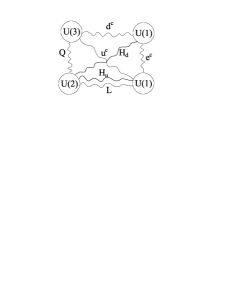
($N=2$)                ($N=3$)

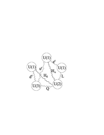
Figure 1: Possible $N=2,3$ brane configurations ($N$ is the number of the $U(1)$-branes) that can accommodate the SM spectrum with down quarks and leptons acquiring masses from the same Higgs doublet.

3 Concrete brane configurations

We consider here brane configurations that can lead to concrete realizations of those proposed previously. As already mentioned, a specific realization must include two Higgs doublets in order to ensure the bottom-top mass difference. In brane models each SM particle corresponds to an open string stretched between two branes. In our charge conventions, the possible quantum numbers of such a string ending to the $U(m)$ and $U(n)$ brane sets are $\left({\bf m};+1,{\bf n};+1\right),\left({\bf\bar{m}};-1,{\bf n};+1\right)$, $\left({\bf m};+1,{\bf\bar{n}};-1\right)$, $\left({\bf\bar{m}};-1,{\bf\bar{n}};-1\right)$, that is, bifundamentals of the associated unitary groups. Higher representations could be obtained by considering strings with both ends on the same brane set $U(m)$, $\left({\bf m(m-1)/2},2\right)$, $\left({\bf m(m+1)/2},2\right)$, $\dots$, however, we will restrict here to the bi-fundamental case. By analyzing possible brane configurations that can accommodate a gauge group of the form (1) we find that only the four and five brane-stack scenarios ($N=2,3$) in (1) can lead to natural $b$-$\tau$ unification. It is possible to introduce additional brane sets, however, in such a case down quarks and leptons get their masses from different Higgs doublets and any Yukawa coupling unification condition would require the equality of the associated doublet vevs. The $N=2,3$ two Higgs doublet candidate configurations are presented pictorially in figure 1.

The associated hypercharge embeddings can be obtained by solving the hypercharge assignment conditions for SM particles for $k_{i}$. SM particle abelian charges under $U_{3}(1)\times U_{2}(1)\times{U(1)}_{1}\times{U(1)}_{2}$ are the general form $Q(+1,\epsilon_{1},0,0)$, $d^{c}(-1,0,\epsilon_{2},0)$, $u^{c}(-1,0,0,\epsilon_{3})$, $L(0,\epsilon_{4},0,\epsilon_{5})$, $e^{c}(0,0,\epsilon_{6},\epsilon_{7})$ and thus

$$k_{3}+k_{2}\,\epsilon_{1} = \hphantom{+}\frac{1}{6}$$

$$-k_{3}+k_{1}^{\prime}\,\epsilon_{2} = \hphantom{+}\frac{1}{3}$$

$$-k_{3}+k\,\epsilon_{3} = -\frac{2}{3}$$ (5)

$$k_{2}\,\epsilon_{4}+k_{2}^{\prime}\,\epsilon_{5} = -\frac{1}{2}$$

$$k_{1}^{\prime}\,\epsilon_{6}+k_{2}^{\prime}\,\epsilon_{7} = \hphantom{+}1$$

where $k=k_{2}^{\prime}$ in the first configuration and $k=k_{3}^{\prime}$ for the second one, while $\epsilon_{i}^{2}=1,\,i=1,\dots,7$. As seen by (2) and (3), only the absolute values of the hypercharge embedding coefficients $k_{i},\,k_{i}^{\prime}$ enter the coupling relation at $M_{S}$. Solving (5), for the SM particle charges in configuration ($N=2$) we obtain three possible solutions. These correspond to the (absolute) values for the coefficients presented in cases (a), (b) and (c) of table 1. Configuration $N=3$ leads to four additional cases, namely (d), (e), (f) and (g) of the same table. If in a particular solution a coefficient $k_{i}$ (or $k_{i}^{\prime}$) turns out to be zero, the associated abelian factor does not participate to the hypercharge.

Table 1: Absolute values of the possible hypercharge embedding coefficient sets ($k_{3},k_{2}$ and $k_{i}^{\prime}$) for the brane configurations with $N=2$ and $N=3$ of figure 1.

$N$		$|k_{3}|$	$|k_{2}|$	$|k_{1}^{\prime}|$	$|k_{2}^{\prime}|$	$|k_{3}^{\prime}|$
	(a)	$\frac{1}{6}$	$0$	$\frac{1}{2}$	$\frac{1}{2}$	-
$2$	(b)	$\frac{2}{3}$	$\frac{1}{2}$	$1$	$0$	-
	(c)	$\frac{1}{3}$	$\frac{1}{2}$	$0$	$1$	-
	(d)	$\frac{1}{6}$	$0$	$\frac{1}{2}$	$\frac{1}{2}$	$\frac{1}{2}$
	(e)	$\frac{1}{3}$	$\frac{1}{2}$	$0$	$1$	$1$
$3$	(f)	$\frac{5}{6}$	$1$	$\frac{1}{2}$	$\frac{1}{2}$	$\frac{3}{2}$
	(g)	$\frac{2}{3}$	$\frac{1}{2}$	$1$	$0$	0

4 Gauge coupling running and the String scale

Following a bottom-up approach, in this section we determine the range of the string scale for all the above models by taking into account the experimental values of $\alpha_{3},\alpha_{e}$ and $\sin^{2}\theta_{W}$ at $M_{Z}$ [22]

$$\alpha_{3}=0.118\pm 0.003,~{}~{}~{}\alpha^{-1}_{e}=127.906,~{}~{}~{}\sin^{2}\theta_{W}=0.23120$$

For the scales above $M_{Z}$ we consider the standard model spectrum with two Higgs doublets. The one loop RGEs for the gauge couplings ($\tilde{\alpha}\equiv\alpha/(4\pi)$) take the form

$$\frac{d\tilde{\alpha}_{i}}{dt}=b_{i}\tilde{\alpha}_{i}^{2}\,,~{}~{}~{}~{}i=Y,2,3$$ (6)

where $(b_{Y},b_{2},b_{3})=(7,-3,-7)$ and $t=2\ln\mu$ ($\mu$ is the renormalization point).

Table 2: Possible values of $k_{Y}$ as a function of $\xi=\alpha_{2}/\alpha_{3}$ for various orientations of $U(1)$’s for the models of table 1. The rows show the $k_{Y}$ values for various orientations (see text for details). Last row shows the minimum value of the string scale $M_{S}$ obtained for the models (a)-(g).

	Model
coupling relation	(a)	(b)	(c)	(d)	(e)	(g)
$\alpha_{i}^{\prime}=\alpha_{2}$	$\frac{\xi}{6}+1$	$\frac{8\xi}{3}+3$	$\frac{2\xi}{3}+3$	$\frac{\xi}{6}+\frac{3}{2}$	$\frac{2\xi}{3}+5$	$\frac{8\xi}{3}+3$
$\alpha_{i}^{\prime}=\alpha_{3}$	$\frac{7\xi}{6}$	$\frac{1\bf{4\xi}}{3}+1$	$\frac{8\xi}{3}+1$	$\frac{2\xi}{3}+1$	$\frac{14\xi}{3}+1$	$\frac{14\xi}{3}+1$
(see text)	$\frac{2\xi}{3}+\frac{1}{2}$	-	-	$\frac{5\xi}{3}$	$\frac{8\xi}{3}+3$	-
(see text)	-	-	-	$\frac{7\xi}{6}+\frac{1}{2}$	-	-
$M_{S}$(GeV)	$6.71\times 10^{17}$	$5.78\times 10^{3}$	$1.99\times 10^{6}$	$1.65\times 10^{14}$	$5.78\times 10^{3}$	$5.78\times 10^{3}$

First, we concentrate on simple relations of the gauge couplings, i.e., those relations implied from models arising only in the context on non-intersecting branes. In these cases, certain constraints on the initial values of the gauge couplings have to be taken into account, leading to a discrete number of admissible cases which we are going to discuss. Thus, in the case of two $D5$ branes, $U(3)$ and $U(2)$ are confined in different bulk directions. In the parallel brane scenario the orientation of a number of the extra $U(1)$’s may coincide with the $U(3)$-stack direction while the remaining abelian branes are parallel to the $U(2)$ stack. This implies that the corresponding $U(1)$ gauge couplings have the same initial values either with the $\alpha_{3}$ or with the $\alpha_{2}$ gauge couplings. If we define $\xi=\frac{\alpha_{2}}{\alpha_{3}}$ the ratio of the two non-abelian gauge couplings at the string scale, for any distinct case, $k_{Y}$ takes the form $k_{Y}=\lambda\,\xi+\nu$, where $\lambda,\nu$ are calculable coefficients which depend on the specific orientation of the $U(1)$ branes. For example, in model (a) we can have the following possibilities: $\alpha_{1}^{\prime}=\alpha_{2}^{\prime}=\alpha_{2}$, $\alpha_{1}^{\prime}=\alpha_{2}^{\prime}=\alpha_{3}$ and $\alpha_{1}^{\prime}=\alpha_{2},\alpha_{2}^{\prime}=\alpha_{3}$ leading to $k_{Y}=\frac{\xi}{6}+1$, $\frac{7\xi}{6}$ and $\frac{2\xi}{3}+\frac{1}{2}$ correspondingly. All cases for the models (a)-(g) are presented in table 2 and are classified with regard to the hypercharge coefficient $k_{Y}$. (All cases of Model (f) lead to unacceptably small string scales, so these are not presented).

Allowing ${\alpha_{3}}$ to take values different from ${\alpha_{2}}$, we find that models (a,b,c,d,e,g) of table 1 predict a string scale in a wide range, from a few TeV up to the Planck mass. The highest value is of the order $M_{S}\sim 7\times 10^{17}$ GeV and corresponds to equal couplings $\frac{\alpha_{2}}{\alpha_{3}}\equiv\xi=1$ at $M_{S}$. On the other hand, lower unification values of the order of a few TeV assume a gauge coupling ratio $\frac{\alpha_{3}}{\alpha_{2}}\approx 2$. In this case the idea of complete gauge coupling unification could be still valid, considering that the SM gauge group arises from the breaking of a gauge symmetry whose non-abelian part is $U(3)\times U(2)^{2}$, i.e., for the case $p=1,\,q=2$ of (1) where the factor of 2 in the gauge coupling ratio is related to the diagonal breaking $U(2)\times U(2)\rightarrow U(2)$. The lowest possible unification for the three models (b),(e),(g) corresponds to $k_{Y}=\frac{14\,\xi}{3}+1$, and is $M_{S}\sim 5.81\times 10^{3}$ GeV, for a weak to strong gauge coupling ratio $\xi\sim 0.42$ at $M_{S}$. Case (c) predicts an intermediate value $M_{S}=2\times 10^{6}$ GeV while model (d) gives $M_{S}\sim 10^{14}$ GeV. Finally, model (a) for $\xi\sim 1$ predicts a unification scale as high as $M_{S}\sim 6.7\times 10^{17}$ GeV which is of the order of the heterotic string scale. Interestingly, in this latter case, all gauge couplings are equal at $M_{S}$, $\alpha_{3}=\alpha_{2}=\alpha_{i}^{\prime}$, while, as can be seen from table 2, $k_{Y}$ takes a common value for all three cases, $k_{Y}=7/6$.

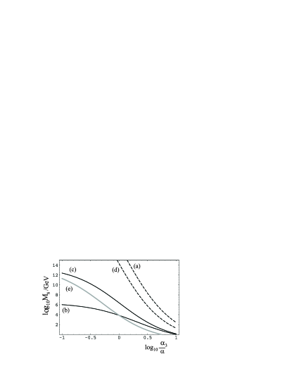
Figure 2: The string scale as a function of the coupling ratio $\frac{\alpha_{3}}{\alpha}$, ($\alpha$ is a common value for the $U(1)$ couplings $\alpha_{i}^{\prime}$) for the hypercharge embeddings of table 1, in the general case of intersecting branes. Results for model (g) coincide with those of model (b).

In the general intersecting case, the $U(1)$ branes are neither aligned to the $SU(3)$, nor to the $SU(2)$ stacks, thus the corresponding gauge couplings can take arbitrary values. Without loss of generality, we will assume here for simplicity that all these couplings are equal $\alpha_{1}^{\prime}=\alpha_{2}^{\prime}=\dots=\alpha_{N}^{\prime}=\alpha$. In figure 2 we plot the string scale ($M_{S}$) as a function of the logarithm of the ratio $\alpha_{3}/\alpha$ for the candidate models (a), (b), (c), (d), (e) and (g). The results for models (b), (c), (e) and (g) which is identical with model (b), are represented in the figure with continuous lines. These are compatible with low scale unification particularly when $\alpha_{3}\geq\alpha$. For $\alpha_{i}^{\prime}=\alpha_{3}$, (which corresponds to the zero of the logarithm at the $x$-axis), we obtain again the results of the parallel brane scenario, shown in table 2. At this point, we further observe a crossing of the (e)-curve with the curve for models (b),(g). It is exactly this point ($\alpha_{i}^{\prime}=\alpha_{3}$) that these three models predict the same value for the lowest string scale. When $\alpha_{3}\geq\alpha_{i}^{\prime}$, model (e) predicts the lowest $M_{S}$, whilst, if $\alpha_{i}^{\prime}>\alpha_{3}$, models (b), (g) imply lower string scales than model (e).

The values of the string scale for models (a), (d) (represented in the figure with dashed curves) are substantially higher; for these latter cases in particular, assuming reasonable gauge coupling relations $\alpha_{i}^{\prime}\approx{\cal O}(\alpha_{2,3})$ we find that $M_{S}\geq 10^{12}$ GeV. Again, for $\alpha_{3}=\alpha_{i}^{\prime}$, (the zero value of the $x$-axis) we rederive the values of $M_{S}$ presented in table 2.

5 Yukawa coupling evolution and mass relations

In this section, we will examine whether a unifiaction of the $b-\tau$ Yukawa couplings is possible in the above described low string scale models. Our procedure is the following: Using the experimentally determined values for the third generation fermion masses $m_{b},m_{\tau}$ we run the 2-loop system of the $SU(3)_{C}\times U(1)_{Y}$ renormalization group equations up to the weak scale ($M_{Z}$) and reconcile there the results with the experimentally known values for the weak mixing angle and the gauge couplings. For the renormalization group running below $M_{Z}$ we define the parameters

$$\tilde{\alpha}_{e}\;=\;\left(\frac{e}{4\pi}\right)^{2},\,\tilde{\alpha}_{3}\;=\;\left(\frac{g_{3}}{4\pi}\right)^{2},\,t\;=\;2\ln\mu$$ (7)

where $e,g_{3}$ are the electromagnetic and strong couplings respectively and $\mu$ is the renormalization scale. The relevant RGEs are [24]

$$\frac{d\tilde{\alpha}_{e}}{dt} = \frac{80}{9}\tilde{\alpha}_{e}^{2}+\frac{464}{27}\tilde{\alpha}_{e}^{3}+\frac{176}{9}\tilde{\alpha}_{e}^{2}\tilde{\alpha}_{3}$$

$$\frac{d\tilde{\alpha}_{3}}{dt} = -\frac{23}{3}\tilde{\alpha}_{3}^{2}-\frac{116}{3}\tilde{\alpha}_{3}^{3}+\frac{22}{9}\tilde{\alpha}_{3}^{2}\tilde{\alpha}_{e}-\frac{9769}{54}\tilde{\alpha}_{3}^{4}$$

$$\frac{dm_{b}}{dt} = m_{b}\left\{-\frac{1}{3}\tilde{\alpha}_{e}-4\tilde{\alpha}_{3}+\frac{397}{162}\tilde{\alpha}_{e}^{2}-\frac{1012}{18}\tilde{\alpha}_{3}^{2}-\frac{4}{9}\tilde{\alpha}_{3}\tilde{\alpha}_{e}-474.8712\tilde{\alpha}_{3}^{3}\right\}$$

$$\frac{dm_{\tau}}{dt} = m_{\tau}\left\{-3\tilde{\alpha}_{e}+\frac{373}{18}\tilde{\alpha}_{e}^{2}\right\}$$

where $m_{b},m_{\tau}$ are the running masses of the bottom quark and the tau lepton respectively, while we use the notation $\tilde{a}_{i}\equiv g^{2}_{i}/16\pi^{2}$ and $\tilde{a}_{t,b,\tau}\equiv\lambda^{2}_{t,b,\tau}/16\pi^{2}$.

The required value for the running mass of $m_{t}$ at $M_{Z}$ is computed as follows: we formally solve the 1-loop RGE system for ($\tilde{a}_{3}$, $\tilde{a}_{2}$, $\tilde{a}_{Y}$, $\tilde{a}_{t}$, $\tilde{a}_{b}$, $\tilde{a}_{\tau}$) and afterwards we determine the interpolating function for $\tilde{a}_{3}(\mu)$ and $m_{t}(\mu;m_{t}^{z})$ at any scale $\mu$ above $M_{Z}$, where $m_{t}^{z}\equiv m_{t}(M_{Z})$ indicates the dependence on an arbitrary initial condition. The unknown value for $m_{t}^{z}$ is determined by solving numerically the algebraic equation

$$\left[m_{t}(\mu;m_{t}^{z})-\frac{M_{t}}{1+\frac{16}{3}\tilde{a}_{3}(\mu)-2\tilde{a}_{t}(\mu)}\right]_{\mu=M_{t}}=0$$ (8)

We use these results as inputs for the relevant parameters and we run the RGE system to higher scales until the $\tilde{a}_{b}$ and $\tilde{a}_{\tau}$ Yukawa couplings coincide. The scale that this happens is considered as the string scale. There, the values of $\tilde{a}_{3},\tilde{a}_{2},\tilde{a}_{Y}$ are checked and the ratio $\tilde{a}_{2}/\tilde{a}_{Y}$ is calculated in order to obtain the normalization constant $k_{Y}$. In our numerical analysis we use for the gauge couplings the values presented in the previous section, for the bottom quark mass $m_{b}$ the experimentally determined range at the scale $\mu=m_{b}$ ie. $m_{b}(m_{b})=4.25\pm 0.15$ GeV and finally the top pole mass is taken to be $M_{t}=178.0\pm 4.3$ GeV [22].

For the scales above $M_{Z}$ we consider the standard model spectrum augmented by one more Higgs. The Higgs doubling is in accordance with the situation that usually arises in the SM variants with brane origin. Moreover, we assume that one Higgs $H_{u}$ only couples to the top quark while the second Higgs $H_{d}$ couples only to the bottom. Then, in analogy with supersymmetry we define the angle $\beta$ related to their vevs where $\tan\beta=\frac{v_{u}}{v_{d}}$. Thus, we have the equations for the gauge couplings

$$\frac{d\tilde{\alpha}_{Y}}{dt}\;=\;7\tilde{\alpha}_{Y}^{2},\;\;\frac{d\tilde{\alpha}_{2}}{dt}\;=\;-3\tilde{\alpha}_{2}^{2},\;\;\frac{d\tilde{\alpha}_{3}}{dt}\;=\;-7\tilde{\alpha}_{3}^{2}$$

and for the Yukawas

$$\frac{d\tilde{\alpha}_{t}}{dt} = \tilde{\alpha}_{t}(-\frac{17}{12}\tilde{\alpha}_{Y}-\frac{9}{4}\tilde{\alpha}_{2}-8\tilde{\alpha}_{3}+\frac{9}{2}\tilde{\alpha}_{t}+\frac{1}{2}\tilde{\alpha}_{b})$$

$$\frac{d\tilde{\alpha}_{b}}{dt} = \tilde{\alpha}_{b}(-\frac{5}{12}\tilde{\alpha}_{Y}-\frac{9}{4}\tilde{\alpha}_{2}-8\tilde{\alpha}_{3}+\frac{1}{2}\tilde{\alpha}_{t}+\frac{9}{2}\tilde{\alpha}_{b}+\tilde{\alpha}_{\tau})$$

$$\frac{d\tilde{\alpha}_{\tau}}{dt} = \tilde{\alpha}_{\tau}(-\frac{15}{4}\tilde{\alpha}_{Y}-\frac{9}{4}\tilde{\alpha}_{2}+3\tilde{\alpha}_{b}+\frac{5}{2}\tilde{\alpha}_{\tau})$$

$$\frac{dv_{u}}{dt} = \frac{v_{u}}{2}(\frac{3}{4}\tilde{\alpha}_{Y}+\frac{9}{4}\tilde{\alpha}_{2}-3\tilde{\alpha}_{t})$$

$$\frac{dv_{d}}{dt} = \frac{v_{d}}{2}(\frac{3}{4}\tilde{\alpha}_{Y}+\frac{9}{4}\tilde{\alpha}_{2}-3\tilde{\alpha}_{b}-\tilde{\alpha}_{\tau})$$

where $t=2\ln\mu$.

Further, if we define $v^{2}=v_{u}^{2}+v_{d}^{2}$, with $v_{u}=v\sin\beta$, $v_{d}=v\cos\beta$ and $v\sim 174~{}{\rm GeV}$, the $Z$-boson mass is given by $M_{Z}^{2}=\frac{1}{2}(g_{Y}^{2}+g_{2}^{2})v^{2}$. The elecromagnetic and the strong couplings are defined in the usual way

$$\tilde{\alpha}_{e}=\tilde{\alpha}_{Y}\cos^{2}\theta_{W}=\tilde{\alpha}_{2}\sin^{2}\theta_{W}$$

while the top and bottom quark masses are related to the Higgs vevs by

$$m_{t}=4\pi v_{u}\sqrt{\tilde{\alpha}_{t}}~{}~{}~{}~{}~{}~{}~{}~{}m_{b}=4\pi v_{d}\sqrt{\tilde{\alpha}_{b}}$$

Table 3: The String scale and the $b-\tau$ ratio at $M_{S}$ for various orientations of $U(1)$ branes presented in table 2.

model	$k_{Y}$	$\xi=\frac{\alpha_{2}}{\alpha_{3}}$	${M_{S}}/{GeV}$	$\frac{m_{b}}{m_{\tau}}(M_{S})$
b,e,g	$2.969$	0.42	$5.786\times 10^{3}$	1.25
c	$2.539$	0.58	$1.986\times 10^{6}$	1.01
d	$1.554$	0.93	$1.645\times 10^{14}$	0.73
a	$1.226$	1.01	$6.710\times 10^{17}$	0.68

We will examine the possibility of obtaining $b-\tau$ unification at a low string scale $M_{S}$. We first concentrate in the models (a)-(g) discussed in the previews section. We present our results in the last column of table 3. We notice that $b-\tau$ unification is obtained in model $c$, for $M_{S}\approx 10^{6}$ GeV. Models (b), (e), (g) with unification scale $M_{S}\approx 5.8\times 10^{3}$ GeV predict a small deviation from exact $b-\tau$ unification. We observe that in these cases the strong-weak gauge coupling ratio is ${a_{3}}\approx 2\,{a_{2}}$.

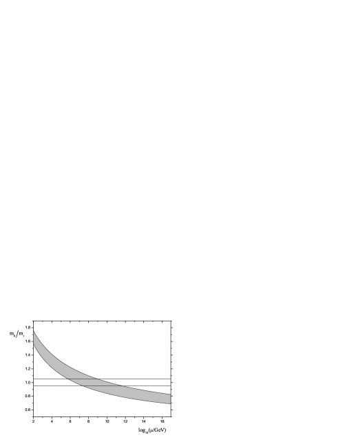
Figure 3: The ratio $\frac{m_{b}}{m_{\tau}}$ as a function of the energy $\mu$ in the 2-Higgs Standard Model. The shaded region corresponds to $a_{3}$ and threshold uncertainties.

In figure 3 the ratio $m_{b}/m_{\tau}$ is plotted as a function of the energy scale for the case of the two-Higgs Standard Model (see [25] and references therein). All previous uncertainties are incorporated and the result is the shaded region shown in the figure. The horizontal shaded band is defined between the values $\frac{m_{b}}{m_{\tau}}=[0.95-1.05]$ and take into account deviations of the ratio $\frac{m_{b}}{m_{\tau}}$ from unity due to possible threshold as well as mixing effects in the full $3\times 3$ quark and lepton flavor mass matrices. As can be seen, exact $m_{b}=m_{\tau}$ equality is found around the scale $M_{S}\approx 10^{6}$ GeV. Taking into consideration $m_{b}/m_{\tau}$-uncertainties expressed through the shaded band, the $M_{S}$ energy range is extended up to $\sim 10^{12}$ GeV.

6 Conclusions

We performed a systematic study of the Standard Model embedding in brane configurations with $U(3)\times U(2)\times U(1)^{N}$ gauge symmetry and we examined a number of interesting phenomenological issues. Seeking for models with economical Higgs sector, we identified two brane configurations with two or three extra abelian branes which can accommodate the Standard Model with two Higgs doublets. We analysed the possible hypercharge embeddings and found seven possible solutions leading to six models (with acceptable string scale $M_{S}$), implying the correct charge assignments for all standard model particles.

We further examined the gauge coupling evolution in these models for both, parallel, as well as intersecting branes and determined the lowest string scale allowed for all possible alignments of the $U(1)$ branes with respect to the $U(3)$ and $U(2)$ non-abelian factors of the gauge symmetry. In the parallel brane scenario, we have identified three models which allow a string scale $M_{S}$ as low as a few TeV, one model with string scale of the order $10^{6}$ GeV and two models with high unification scales. Similar results were obtained for the general case of intersecting branes.

We further analysed the consequences of the third generation fermion mass relations and in particular $b-\tau$ equality at the string scale on the above models. In the parallel brane scenario, we found that exact $b-\tau$ Yukawa unification is obtained only in the model with $M_{S}\approx 10^{3}$ TeV, while in the TeV string scale models the $m_{b}/m_{\tau}$ ratio deviates from unity by $25\%$. Allowing the $U(1)$ gauge couplings to take arbitrary (perturbative) values, we found that $b-\tau$ Yukawa unification is possible for a wide string scale range form $10^{6}$ up to $10^{12}$ GeV.

This research was funded by the program ‘PYTHAGORAS’ (no. 1705 project 23) of the Operational Program for Education and Initial Vocational Training of the Hellenic Ministry of Education under the 3rd Community Support Framework and the European Social Fund.

References

References

- [1] Antoniadis I 1990 Phys. Lett. B 246 377
- [2] Arkani-Hamed N, Dimopoulos S and Dvali G R 1998 Phys. Lett. B 429 63 (Preprint hep-ph/9803315)
- [3] Antoniadis I, Arkani-Hamed N, Dimopoulos S and Dvali G R 1998 Phys. Lett. B 436 257
- [4] Lykken J D 1996 Phys. Rev. D 54 3693 (Preprint hep-th/9603133)
- [5] Polchinski J (Preprint hep-th/9611050)
- [6] Angelantonj C and Sagnotti A 2002 Phys. Rept. 371 1 [Erratum 2003 ibid. 376 339]
- [7] Berkooz M, Douglas M R and Leigh R G 1996 Nucl. Phys. B 480 265 (Preprint hep-th/9606139)
- [8] Balasubramanian V and Leigh R G 1997 Phys. Rev. D 55 6415 (Preprint hep-th/9611165)
- [9] Antoniadis I, Kiritsis E and Tomaras T N 2000 Phys. Lett. B 486 186 (Preprint hep-ph/0004214)
- [10] Antoniadis I, Kiritsis E, Rizos J and Tomaras T N 2003 Nucl. Phys. B 660 81 (Preprint hep-th/0210263)\nonumCoriano C, Irges I and Kiritsis E (Preprint hep-ph/0510332)
- [11] Antoniadis I, Kiritsis E and Rizos J 2002 Nucl. Phys. B 637 92 (Preprint hep-th/0204153)
- [12] Gioutsos D V, Leontaris G K and Rizos J 2006 Eur. Phys. J. C 45 241 (Preprint hep-ph/0508120)
- [13] Aldazabal G, Franco S, Ibanez L E, Rabadan R and Uranga A M 2001 JHEP 0102 047\nonumIbanez L E, Marchesano F and Rabadan R 2001 JHEP 0111 002 (Preprint hep-th/0105155)\nonumBlumenhagen R, Kors B, Lust D and Ott T 2001 Nucl. Phys. B 616 3 (Preprint hep-th/0107138)
- [14] Cvetic M, Shiu G and Uranga A M 2001 Phys. Rev. Lett. 87 201801 (Preprint hep-th/0107143)\nonumCvetic M, Shiu G and Uranga A M 2001 Nucl. Phys. B 615 3 (Preprint hep-th/0107166)\nonumBlumenhagen R, Cvetic M, Langacker P and Shiu G (Preprint hep-th/0502005)
- [15] Leontaris G K and Rizos J 2001 Phys. Lett. B 510 295 (Preprint hep-ph/0012255)
- [16] Kokorelis C 2002 JHEP 0208 018 (Preprint hep-th/0203187)\nonumKokorelis C 2004 Nucl. Phys. B 677 115 (Preprint hep-th/0207234)\nonumEverett L L, Kane G L, King S F, Rigolin S and Wang L T 2002 Phys. Lett. B 531 263\nonumBranco G C, Gerard J M, Gonzalez F R and Nobre B M (Preprint hep-ph/0305092)\nonumAxenides M, Floratos E and Kokorelis C 2003 JHEP 0310 006 Preprint hep-th/0307255)
- [17] Blumenhagen R, Lust D and Stieberger S 2003 JHEP 0307 036 (Preprint hep-th/0305146)\nonumBlumenhagen R, Cvetic M, Marchesano F and Shiu G 2005 JHEP 0503 050 (Preprint hep-th/0502095)
- [18] Blumenhagen R, Cvetic M, Langacker P and Shiu G (Preprint hep-th/0502005)\nonumCremades D, Ibanez L E and Marchesano F 2004 JHEP 0405 079 (Preprint hep-th/0404229)\nonumAnastasopoulos P (Preprint hep-th/0503055)
- [19] Antoniadis I and Dimopoulos S 2005 Nucl. Phys. B 715 120 (Preprint hep-th/0411032)\nonumGioutsos D V, Leontaris G K and Psallidas A (Preprint hep-ph/0605187)
- [20] Chanowitz M S, Ellis J R and Gaillard M K 1977 Nucl. Phys. B 128 506\nonumBuras A J, Ellis J R, Gaillard M K and Nanopoulos D V 1978 Nucl. Phys. B 135 66\nonumAnanthanarayan B, Lazarides G and Shafi Q 1991 Phys. Rev. D 44 1613\nonumCarena M, Olechowski M, Pokorski S and Wagner C E M 1994 Nucl. Phys. B 426 269
- [21] Greene B R, Kirklin K H, Miron P J and Ross G G 1987 Nucl. Phys. B 292 606\nonumAntoniadis I and Leontaris G K 1989 Phys. Lett. B 216 333\nonumAntoniadis I, Leontaris G K and Rizos J 1990 Phys. Lett. B 245 161\nonumFaraggi A E 1992 Phys. Lett. B 274 47\nonumCleaver G, Cvetic M, Espinosa J R, Everett L L, Langacker P and Wang J 1999 Phys. Rev. D 59 115003\nonumLeontaris G K and Rizos J 1999 Nucl. Phys. B 554 3 (Preprint hep-th/9901098)
- [22] Eidelman S et al. 2004 Phys. Lett. B 592 1
- [23] Parida M K and Usmani A 1996 Phys. Rev. D 54 3663\nonumDas C R and Parida M K 2001 Eur. Phys. J. C 20 121 (Preprint hep-ph/0010004)
- [24] Arason H, Castano D J, Keszthelyi B, Mikaelian S, Piard E J, Ramond P and Wright B D 1992 \PRD 46 3945
- [25] Kane G L, King S F, Peddie I N R and Velasco-Sevilla L 2005 JHEP 0508 083 (Preprint hep-ph/0504038)