Holographic Wave Functions, Meromorphization and Counting Rules

Abstract

We study the large-$Q^{2}$ behavior of the meson form factor $F_{M}(Q^{2})$ constructed using the holographic light-front wave functions proposed recently by Brodsky and de Teramond. We show that this model can be also obtained within the Migdal’s regularization approach (“meromorphization”), if one applies it to 3-point function for scalar currents made of scalar quarks. We found that the asymptotic $1/Q^{2}$ behavior of $F_{M}(Q^{2})$ is generated by soft Feynman mechanism rather than by large transverse momentum dynamics, which causes very late onset of the $1/Q^{2}$ asymptotic behavior. It becomes visible only for unaccessible momenta $Q^{2}\gtrsim 10$  GeV². Using meromorphization for spin-1/2 quarks, we demonstrated that resulting form factor $F^{\rm spinor}_{M}(Q^{2})$ has $1/Q^{4}$ asymptotic behavior. Now, owing to the late onset of this asymptotic pattern, $F^{\rm spinor}_{M}(Q^{2})$ imitates the $1/Q^{2}$ behavior in the few GeV² region. We discuss analogy between meromorphization and local quark-hadron duality model for the pion form factor, and show that adding the ${\cal O}(\alpha_{s})$ correction to the spectral function brings in the hard pQCD contribution that has the dimensional counting $1/Q^{2}$ behavior at large $Q^{2}$. At accessible $Q^{2}$, the ${\cal O}(\alpha_{s})$ term is a rather small fraction of the total result. In this scenario, the “observed” quark counting rules for hadronic form factors is an approximate phenomenon resulting from Feynman mechanism in its preasymptotic regime.

I Introduction

Experimental evidence that form factors of hadrons consisting of $n$ quarks have behavior close to $1/(Q^{2})^{n-1}$, provokes expectations that there is a fundamental and/or easily visible reason for such a phenomenon, scale invariance being the most natural suspect. Indeed, for an elementary fermion, EM form factor is constant, $\langle P^{\prime}|J^{\mu}|P\rangle=\bar{u}(P^{\prime})\gamma^{\mu}u(P)$. When $(n-1)$ spectator quark fields with dimension (mass)^3/2 are added to the initial state $|P\rangle$ and the final state $\langle P^{\prime}|$, the extra kinematical factors $\sim[u(P)\bar{u}(P^{\prime})]^{n-1}$ take only worth of (mass)^(n-1), and a constant of dimension (mass)^2(n-1) is needed to take care of the rest. If, except for this overall constant, no other dimensionful constants can show up for large $Q^{2}$, then form factor has the quark counting rule $1/(Q^{2})^{n-1}$ behavior Matveev:1977ra . A specific dynamical mechanism Brodsky:1973kr that produces a scale invariant behavior is provided by hard rescattering in a theory with dimensionless coupling constant. After advent of QCD, pion and nucleon form factors were calculated within the hard scenario Farrar:1979aw ; Chernyak:1977fk ; Radyushkin:1977gp ; Lepage:1979zb , and it was realized that perturbative QCD predicts, in fact, the $(\alpha_{s}/Q^{2})^{n-1}$ asymptotic behavior. In the pion case, the prediction is $F_{\pi}(Q^{2})=(2\alpha_{s}/\pi)s_{0}/Q^{2}$, where $s_{0}=4\pi^{2}f_{\pi}^{2}\approx 0.7$ GeV² is a constant close to $m_{\rho}^{2}\approx 0.6$ GeV². This indicates that the pQCD asymptotics is not the large-$Q^{2}$ limit of the phenomenologically successfull VMD fit $F_{\pi}^{\rm VMD}(Q^{2})\sim 1/(1+Q^{2}/m_{\rho}^{2})$, but rather looks like ${\cal O}(\alpha_{s})$ correction to it. Also, the smallness of $\alpha_{s}/\pi$ undermines attempts to describe available data solely by pQCD hard mechanism. During the last years, the growing consensus is that at available $Q^{2}$, form factors are dominated by soft contributions described by nonforward parton densities ${\cal F}(x,Q^{2})$ Radyushkin:1998rt (or generalized parton distributions $H(x,\xi;Q^{2})$ for zero skewness $\xi$), and successful fits were obtained Belitsky:2003nz ; Diehl:2004cx ; Guidal:2004nd in models with ${\cal F}(x,Q^{2})=f(x)\,e^{-Q^{2}g(x)}$ having exponential behavior for large $Q^{2}$ at fixed $x$. If $g(x)$ vanishes for $x\to 1$ like $(1-x)^{a}$, a powerlike asymptotics $F(Q^{2})\sim(1/Q^{2})^{(b+1)/a}$ in this case appears only after integration over $x$, i.e., it is governed by the so-called Feynman mechanism Feynman , and is determined by the $x\to 1$ behavior $f(x)\to(1-x)^{b}$ of the preexponential function $f(x)$, in contrast to the hard mechanism for which the subprocess amplitude already has the $(1/Q^{2})^{n-1}$ power behavior not affected by subsequent $x$-integrations.

Another new development is related to applications of AdS/CFT construction to QCD and claims Polchinski:2002jw ; Brodsky:2003px that this framework (often referred as “AdS/QCD”) provides a nonperturbative explanation of quark counting rules. In this scenario, they reflect the conformal invariance of the 5-dimensional theory, in particular, the power behavior of the normalizable modes $\Phi(\zeta)$ at small values of the 5th coordinate $\zeta$. Parametrically, the prediction has the form $(\Lambda^{2}/Q^{2})^{n-1}$, without any accompanying $\alpha_{s}^{n-1}$ factors. Given explicit expressions for $\Phi(\zeta)$, with the value of $\Lambda$ fixed from fitting the hadron masses, it is straightforward to check the structure of AdS/QCD results for form factors and their potential to describe the features of existing data. This is one of the goals of the present investigation. Another is to study the recently proposed interpretation Brodsky:2006uq of AdS/QCD results in terms of light-front wave functions, which opens a possibility to find out whether, in terms of the light-cone momenta $x,{\bf k}_{\perp}$, the AdS/QCD quark counting corresponds to large-${\bf k}_{\perp}$ hard mechanism or, as we will show, to the $x\to 1$ soft Feynman/Drell-Yan Feynman ; Drell:1969km mechanism. In view of yet another recent observation Erlich:2006hq that some of the results of the AdS/QCD approach coincide with those of Migdal’s program Migdal:1977nu (that starts with a perturbative correlator and substitutes its cuts by hadron poles), we apply the extension Dosch:1977qh of this “meromorphization” idea to the 3-current correlators, and establish a connection between this approach and holographic light-front wave functions of Ref. Brodsky:2006uq .

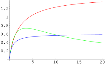
Finally, we discuss analogy between the meromorphization procedure and the “local quark-hadron duality” model Nesterenko:1982gc that succesfully describes the pion form factor data and gives a unified description of its soft and hard parts. The soft term $F_{\pi}^{\rm LD}(Q^{2})$ in this approach dominates at accessible $Q^{2}$, but has the $1/Q^{4}$ asymptotic behavior. Due to its late onset, the curve $Q^{2}F_{\pi}^{\rm LD}(Q^{2})$ has a wide plateau in a few GeV² region, i.e., $F_{\pi}^{\rm LD}(Q^{2})$ imitates there the $1/Q^{2}$ behavior. Thus, the desired $1/Q^{2}$ result for accessible $Q^{2}$ is obtained because the nonperturbative term has a faster, $1/Q^{4}$ asymptotic fall-off. On the other hand, the curve $Q^{2}F_{M}(Q^{2})$ for the meson form factor in the holographic model of Ref. Brodsky:2006uq monotonically increases to its asymptotic value $\sim 2.6\,m_{\rho}^{2}$, and is far from being flat in the whole accessible region $Q^{2}\lesssim 10$ GeV².

II Holographic wave functions

We will need some elements of the derivation of the holographic wave functions proposed in Ref. Brodsky:2006uq . In the hard-wall approximation Polchinski:2002jw , the expression for the elastic form factor in the holographic duality model is given by

$$F(Q^{2})=\int_{0}^{1/\Lambda}\frac{d\zeta}{\zeta^{3}}\,\Phi_{P^{\prime}}(\zeta)J(Q,\zeta)\Phi_{P}(\zeta)\ ,$$ (1)

where $J(Q,\zeta)=\zeta QK_{1}(\zeta Q)$ is the “nonnormalizable” mode describing the EM current, and $\Phi_{P}(\zeta)$, $\Phi_{P^{\prime}}(\zeta)$ come from the “normalizable” modes describing initial and final states, with $\Phi(\zeta)=C\zeta^{2}J_{L}(\beta_{L,k}\zeta\Lambda)$ for a $\bar{q}q$ state with orbital momentum $L=0,1,\ldots$ and radial number $k=1,2,\ldots$, and $\beta_{L,k}$ being the $k$th root of the Bessel function $J_{L}(x)$. On the other hand, in the light-cone (LC) formalism,

$$F(Q^{2})=\int^{1}_{0}dx\int d^{2}{\bf\eta}_{\perp}e^{i{\bf\eta}_{\perp}\cdot{\bf q}_{\perp}}{\cal B}(x,{\bf\eta}_{\perp})\equiv\int^{1}_{0}dx\,{\cal F}(x,Q^{2}),$$ (2)

where ${\cal B}(x,{\bf\eta}_{\perp})$ is a parton density function Soper:1976jc that depends on $x$, the light-cone momentum fraction of the active quark, and ${\bf\eta}_{\perp}$, the $x_{i}$-weighted transverse position of spectators. The function ${\cal B}(x,{\bf\eta}_{\perp})$ accumulates information from all Fock components and its ${\bf\eta}_{\perp}$ Fourier transform gives the generalized parton distribution (GPD) ${\cal F}(x,Q^{2})$. In particular, the 2-body part of a meson form factor is given by

$$F_{(2)}(Q^{2})=\int^{1}_{0}dx\int d^{2}{\bf b}_{\perp}e^{i\bar{x}{\bf b}_{\perp}\cdot{\bf q}_{\perp}}\Bigl{|}\Psi_{2}(x,{\bf b}_{\perp})\Bigr{|}^{2}\ ,$$ (3)

where $\bar{x}\equiv 1-x$. With the wave function depending on ${\bf b}_{\perp}$ through $b\equiv|{\bf b}_{\perp}|$ one obtains

$$F_{(2)}(Q^{2})=2\pi\int^{1}_{0}dx\int_{0}^{\infty}bdbJ_{0}(\bar{x}bQ)|\Psi_{2}(x,b)|^{2}=2\pi\int^{1}_{0}\frac{dx}{x\bar{x}}\int_{0}^{\infty}zdzJ_{0}\left(\sqrt{\frac{\bar{x}}{x}}\,z\,Q\right)\,|\phi(x,z)|^{2}\ ,$$ (4)

where $z\equiv\sqrt{x\bar{x}}b$ and wave function was written as $\Psi_{2}(x,b)=\phi(x,z)$. Noticing that the integral

$$\int_{0}^{1}dxJ_{0}\left(\sqrt{\frac{1-x}{x}}\,z\,Q\right)=zQK_{1}(zQ)\equiv{\cal K}_{1}(zQ)=J(Q,z)$$ (5)

gives $J(Q,z)$, and assuming that $|\phi(x,z)|^{2}=x\bar{x}\chi^{2}(z)$, LC formula (4) is cast into the form

$$F(Q^{2})=2\pi\int_{0}^{\infty}zdz\ {\cal K}_{1}(zQ)\,\chi^{2}(z)$$ (6)

that converts into Eq. (1) if one identifies $\Phi(\zeta)\sim\zeta^{2}\chi(\zeta)$. In general case, $z$ is introduced through $|\eta_{\perp}|=z\sqrt{\bar{x}/x}$, and one assumes that ${\cal B}(x,{\bf\eta}_{\perp})=(x/\bar{x})\chi^{2}(z)$. This gives the “holographic” model Brodsky:2006uq for light-front wave functions. By construction, they should guarantee the $F_{M}(Q^{2}=0)=1$ constraint, i.e., they are effective wave functions (see, e.g., Radyushkin:1995pj ) normalized by

$$\int^{1}_{0}dx\int d^{2}{\bf b}_{\perp}|\Psi_{\rm eff}(x,{\bf b}_{\perp})|^{2}\ =1\ ,$$ (7)

unlike the two-body wave functions $\Psi_{2}(x,{\bf b}_{\perp})$ normalized to the probability of finding the meson in the $\bar{q}q$ Fock state. We will focus on the lowest meson having $L=0,k=1$ and mass $M=\beta_{0,1}\Lambda$. Then

$$\Psi_{M}(x,b)=\frac{M\sqrt{x\bar{x}/\pi}}{\beta_{0,1}J_{1}(\beta_{0,1})}\,J_{0}(\sqrt{x\bar{x}}Mb)\,\theta(\sqrt{x\bar{x}}b\leq\beta_{0,1}/M)\ ,$$ (8)

where $\beta_{0,1}J_{1}(\beta_{0,1})\approx 1.2$. The ${\bf k}_{\perp}$ counterpart of this wave function is given by

$$\widetilde{\Psi}_{M}(x,{\bf k}_{\perp})=\frac{1}{2\pi}\int d^{2}{\bf b}_{\perp}e^{-i{\bf b}_{\perp}\cdot{\bf k}_{\perp}}\Psi_{M}(x,{\bf b}_{\perp})=\frac{M}{\sqrt{\pi x\bar{x}}}\,\frac{J_{0}(\beta_{0,1}k_{\perp}/\sqrt{x\bar{x}}M)}{M^{2}-{k_{\perp}^{2}}/{x\bar{x}}}\ .$$ (9)

Figure 1: Momentum wave function $M\sqrt{\pi x\bar{x}}\,\widetilde{\Psi}_{M}(x,{\bf k}_{\perp})$ (lower curve, blue online) as a function of ${k_{\perp}^{2}}/M^{2}{x\bar{x}}$; for comparison also shown $\exp(-{k_{\perp}^{2}}/2M^{2}{x\bar{x}})$ (upper curve, red online).

Since $\beta_{0,1}$ is a root of $J_{0}(z)$, the momentum wave function $\widetilde{\Psi}_{M}(x,{\bf k}_{\perp})$ has no singularities for ${k_{\perp}^{2}}/{x\bar{x}}=M^{2}$, and it has zeros when ${k_{\perp}^{2}}/{x\bar{x}}$ coincides with squared masses of higher states. For large $k_{\perp}$, wave function oscillates with the magnitude decreasing as $1/k_{\perp}^{5/2}$,

$$\widetilde{\Psi}_{M}(x,{\bf k}_{\perp})\sim\,-\frac{M}{{\pi k_{\perp}^{2}}}\,\sqrt{2x\bar{x}}\ \frac{\cos(k_{\perp}/\sqrt{x\bar{x}}\Lambda-\pi/4)}{\sqrt{k_{\perp}/\sqrt{x\bar{x}}\Lambda}}\ .$$ (10)

This result contradicts the statement made in Ref. Brodsky:2003px that the AdS/QCD construction corresponds to a purely power-law large-$k_{\perp}$ behavior $\psi(k_{\perp})\sim(1/k_{\perp}^{2})^{n-1}$ for the wave function of $n$-particle bound state.

III Feynman mechanism

We can get the large-$Q^{2}$ asymptotics of the lowest state form factor

$$F_{M}(Q^{2})=\frac{2M^{2}}{Q^{2}[\beta_{0,1}J_{1}(\beta_{0,1})]^{2}}\int_{0}^{Q/\Lambda}\xi\,{d\xi}\,{\cal K}_{1}(\xi)\,J^{2}_{0}(\xi M/Q)\ ,$$ (11)

by Taylor expanding $J_{0}^{2}(\xi M/Q)$ and neglecting ${\cal O}(e^{-Q/\Lambda})$ terms from the upper limit of $\xi$ integration:

$$F_{M}(Q^{2})=\frac{4M^{2}}{Q^{2}[\beta_{0,1}J_{1}(\beta_{0,1})]^{2}}\left[1-\frac{4M^{2}}{Q^{2}}+\frac{9}{8}\left(\frac{4M^{2}}{Q^{2}}\right)^{2}+{\cal O}(M^{6}/Q^{6})\right]+{\cal O}(e^{-Q/\Lambda})\sim\frac{0.64}{1+Q^{2}/4M^{2}}\ .$$ (12)

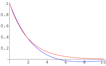
Though this result has a monopole-like structure, the scale $4M^{2}$ is evidently too large. With $M=m_{\rho}$, the curve for $Q^{2}F_{M}(Q^{2})$ is far from being flat in the accessible region $Q^{2}\lesssim 10$  GeV². Note also, that though the large-$Q^{2}$ behavior of $F_{M}(Q^{2})$ is determined by the small-$\zeta$ behavior of $\Phi(\zeta)$, when $\zeta$ is interpreted as $\sqrt{x\bar{x}}b$, the value $\zeta=0$ may correspond to $x=1$ rather than to large transverse momenta. Let us see which mechanism is responsible for the $1/Q^{2}$ asymptotics in terms of the $x,{\bf k}_{\perp}$ Drell-Yan formula Drell:1969km

$$F_{M}(Q^{2})=\int_{0}^{1}dx\int d^{2}{\bf k}_{\perp}\,\widetilde{\Psi}_{M}^{*}(x,{\bf k}_{\perp}+\bar{x}{\bf q}_{\perp})\widetilde{\Psi}_{M}(x,{\bf k}_{\perp})\ ,$$ (13)

$Q\equiv|{\bf q}_{\perp}|$. With $\widetilde{\Psi}_{M}(x,{\bf k}_{\perp})$ decreasing at large ${\bf k}_{\perp}$, there are two possibilities huang (see also Mukherjee:2002gb ):
$a)$ finite $x$ and small $|{\bf k}_{\perp}|$, e.g., the region $|{\bf k}_{\perp}|\ll\bar{x}|{\bf q}_{\perp}|$, where $\widetilde{\Psi}_{M}(x,{\bf k}_{\perp})$ is maximal. This gives

$$F_{M}(Q^{2})\approx\int_{0}^{1}dx\int d^{2}{\bf k}_{\perp}\,|\widetilde{\Psi}_{M}^{*}(x,\bar{x}{\bf q}_{\perp})\,\widetilde{\Psi}_{M}(x,{\bf k}_{\perp})|+\{\widetilde{\Psi}\Leftrightarrow\widetilde{\Psi}^{*}\}\sim 2\int_{0}^{1}{dx}\,|\widetilde{\Psi}_{M}^{*}(x,\bar{x}{\bf q}_{\perp})\,\varphi(x)|\ .$$ (14)

In the hard scenario, when the $x$ integral is not dominated by the $x\to 1$ region, the large-$Q^{2}$ behavior of the form factor repeats the large-$k_{\perp}$ behavior of the momentum wave function. The latter does not behave as $1/k_{\perp}^{2}$: it oscillates with magnitude decreasing as $1/k_{\perp}^{2.5}$, see Eq. (10), so we need to turn to the second possibility:
$b)$ $x$ is close to 1, so that $|\bar{x}{\bf q}_{\perp}|\sim|{\bf k}_{\perp}|$, and $|{\bf k}_{\perp}|$ is small. Then both $\widetilde{\Psi}_{M}(x,{\bf k}_{\perp})$ and $\Psi_{M}^{*}(x,{\bf k}_{\perp}+\bar{x}{\bf q}_{\perp})$ are maximal. In Ref. Drell:1969km , it was argued that the dominant contribution comes from $\bar{x}|{\bf q}_{\perp}|\lesssim m={\rm const}$, and the large-$Q^{2}$ behavior of the form factor in this scenario reflects the phase space available for such configurations. To make a specific estimate, we represent the form factor as the $x$-integral (2) of GPD

$${\cal F}_{M}(x,Q^{2})=\frac{2}{\beta^{2}_{0,1}J_{1}^{2}(\beta_{0,1})}\int_{0}^{\beta_{0,1}}ydy\,J_{0}\left(\sqrt{\frac{\bar{x}}{x}}\,\frac{Q}{M}\,y\right)J_{0}^{2}(y)\equiv{\cal G}(\sigma)\,,$$ (15)

which in this case is a function ${\cal G}(\sigma)$ of $\sigma\equiv\bar{x}Q^{2}/xM^{2}$ (see Fig. 2). The form factor is then given by

$$F_{M}(Q^{2})=\frac{M^{2}}{Q^{2}}\int_{0}^{\infty}d\sigma\,\frac{{\cal G}(\sigma)}{(1+\sigma M^{2}/Q^{2})^{2}}\ ,$$ (16)

and the leading $1/Q^{2}$ term is proportional to zeroth $\sigma$-moment of ${\cal G}(\sigma)$, which does not vanish though the function ${\cal G}(\sigma)$ oscillates for large values of $\sigma$. In fact, it is very small in the region above its first zero (at $\sigma\approx 9$) while in the region below this zero ${\cal G}(\sigma)$ is very close to the exponential $e^{-\sigma/2.6}$, the integration of which gives the correct coefficient for the ${\cal O}(M^{2}/Q^{2})$ term. Thus, the leading large-$Q^{2}$ term is given by integration over $\sigma\lesssim 10$ or, returning to the $x$-variable, by the region $\bar{x}\lesssim 10M^{2}/Q^{2}$ (we see again that asymptotic estimates can be used only for $Q^{2}\gg 4M^{2}$). The $\bar{x}\lesssim{\cal O}(M^{2}/Q^{2})$ result parametrically differs from the estimate given in Ref. Drell:1969km . The reason is that the transverse momentum ${\bf k}_{\perp}$ enters into the wave function through the combination $|{\bf k}_{\perp}|^{2}/x\bar{x}$, and the $x$-size of the dominant region is determined by $|{\bf k}_{\perp}+\bar{x}{\bf q}_{\perp}|^{2}/x\bar{x}M^{2}\lesssim{\rm const}$ or $|\bar{x}{\bf q}_{\perp}|^{2}/x\bar{x}\lesssim{\rm const}\,M^{2}$, which gives $\bar{x}\lesssim{\rm const}\,M^{2}/Q^{2}$.

Figure 2: Generalized parton distribution ${\cal F}_{M}(x,Q^{2})$ (lower curve, blue online) as a function of $\bar{x}Q^{2}/xM^{2}\equiv\sigma$. For comparison, we also show $\exp(-\sigma/3)$ (upper curve, red online).

Thus, we found that the large-$Q^{2}$ asymptotics of the meson form factor in the model of Ref. Brodsky:2006uq is governed by the soft Feynman mechanism, with the power-law asymptotics determined by the $x\to 1$ behavior of the prefactor $f(x)$ accompanying a decreasing function of $\bar{x}Q^{2}/x\Lambda^{2}$. In the present case, $f(x)=1$, which gives $F_{M}(Q^{2})\sim 1/Q^{2}$. With extra $\bar{x}^{N}$ factor, the outcome of the $x$-integration would be $(\Lambda^{2}/Q^{2})^{N+1}$. Clearly, the prefactor $f(x)$ is nothing else but the parton distribution function:

$$f(x)={\cal F}(x,Q^{2}=0)=\int\,d^{2}{\bf b}_{\perp}\,|\Psi(x,{\bf b}_{\perp})|^{2}=\int\,d^{2}{\bf k}_{\perp}\,|\Psi(x,{\bf k}_{\perp})|^{2}\,,$$ (17)

i.e., the model of Ref. Brodsky:2006uq gives a constant, $x$-independent parton distribution $f(x)=1$.

If we approximate $\widetilde{\Psi}_{M}(x,{\bf k}_{\perp})$ by a Gaussian function $\widetilde{\Psi}_{G}(x,{\bf k}_{\perp})\sim\exp[-{k_{\perp}^{2}}/2M^{2}{x\bar{x}}]/\sqrt{x\bar{x}}$ (see Fig. 1), the relevant GPD ${\cal F}_{G}(x,Q^{2})$ can be calculated analytically. It is instructive to perform such a calculation in the impact parameter space. Then $\Psi_{G}(x,b)\sim\sqrt{x\bar{x}}\exp[-{b^{2}}M^{2}{x\bar{x}}/2]$ (in fact, a Gaussian wave function for a ground state is obtained in the hologaphic model of Ref. Karch:2006pv that gives a linear law for (mass)² of excited states), and integrating over all (including small) values of ${\bf b}_{\perp}$ in the form factor formula (3) gives ${\cal F}_{G}(x,Q^{2})=e^{-\bar{x}Q^{2}/4xM^{2}}$, a function that, for any fixed $x$, vanishes exponentially at large $Q^{2}$. The power-law asymptotics is obtained only after integrating over $x$, which gives

$$F_{G}(Q^{2})=\sum_{n=1}^{\infty}(-1)^{n-1}n!\,\left(\frac{4M^{2}}{Q^{2}}\right)^{n}=\frac{4M^{2}}{Q^{2}}\left[1-2\,\left(\frac{4M^{2}}{Q^{2}}\right)+6\,\left(\frac{4M^{2}}{Q^{2}}\right)^{2}+{\cal O}(M^{6}/Q^{6})\right]\ ,$$ (18)

a result that has the ${\cal O}(M^{2}/Q^{2})$ large-$Q^{2}$ behavior and structure similar to that of Eq. (12). The crucial role of integration over the $x\sim 1$ region in getting the power-law behaviour is evident: if the integration is restricted to $x<x_{0}$, the outcome vanishes exponentially (like $\exp[-\bar{x}_{0}Q^{2}/4x_{0}M^{2}]$) for large $Q^{2}$. Thus, the GPD ${\cal F}_{G}(x,Q^{2})$ corresponding to the Gaussian wave function has the same ${\cal F}(x,Q^{2})=f(x)\,e^{-Q^{2}g(x)}$ structure as those considered in Refs. Belitsky:2003nz ; Diehl:2004cx ; Guidal:2004nd .

IV Meromorphization

One may question the conjectures of the model of Ref. Brodsky:2006uq , e.g., the interpretation of the holographic variable $\zeta$ as a particular product $\sqrt{x\bar{x}}b$ of light-cone variables. We are going to show that the picture similar to that of Ref. Brodsky:2006uq emerges also within the approach related to Migdal’s program Migdal:1977nu of Padé approximating the correlators $\Pi(p^{2})$ of hadronic currents calculated in perturbation theory. Recently Erlich:2006hq , it was demonstrated that some of Migdal’s results coincide with those of the holographic approach. Migdal’s program involves “meromorphization”

$$\Pi(p^{2})=\frac{1}{\pi}\int_{0}^{\infty}\frac{\rho(s)}{s-p^{2}}\,ds\Rightarrow\Pi_{\cal M}(p^{2})=\Pi(p^{2})-\frac{1}{\pi{\cal Q}(p^{2})}\int_{0}^{\infty}\frac{\rho(s)\,{\cal Q}(s)}{s-p^{2}}\,ds$$ (19)

that substitutes the original correlator $\Pi(p^{2})$ by a function $\Pi_{\cal M}(p^{2})$ in which the cut of the original correlator for real positive $p^{2}$ is eliminated by the second term in Eq. (19), with zeros of ${\cal Q}(p^{2})$ at timelike $p^{2}$ generating the poles interpreted as hadronic bound states. Explicit Padé construction in case of correlators of currents like the scalar current $\varphi\varphi$ of scalar fields, vector current $\bar{\psi}\gamma_{\mu}\psi$ of spin-1/2 quarks, etc., gives ${\cal Q}(p^{2})\Rightarrow J_{0}(\beta_{0,1}\sqrt{p^{2}}/M),$ with $M$ being the mass of the lowest state. In the deep spacelike region ($p^{2}\equiv-P^{2}\to-\infty$), the difference between the original expression and the approximant then vanishes exponentially like $e^{-2\beta_{0,1}P/M}$. The coupling constant $f_{M}^{2}$ of the lowest state is given by

$$f_{M}^{2}=\lim_{p^{2}\to M^{2}}(M^{2}-p^{2})\,\Pi_{\cal M}(p^{2})=\frac{1}{\pi{\cal Q}^{\prime}(M^{2})}\int_{0}^{\infty}\frac{\rho(s)\,{\cal Q}(s)}{s-M^{2}}\,ds\ .$$ (20)

In the lowest order, $\rho(s)=\rho_{0}\,\theta(s)$, with $\rho_{0}=1/16\pi$ for $j=\varphi\varphi$, and $\rho_{0}=N_{c}/12\pi$ for vector and axial currents $\bar{u}\gamma_{\mu}(\gamma_{5})d$ of spin-1/2 quarks. This gives

$$f_{M}^{2}=\frac{2\rho_{0}M^{2}}{\pi\beta_{0,1}J_{1}(\beta_{0,1})}\int_{0}^{\infty}\frac{J_{0}(\beta_{0,1}\sqrt{s}/M)}{M^{2}-s}\,ds=\frac{4\rho_{0}M^{2}}{\pi[\beta_{0,1}J_{1}(\beta_{0,1})]^{2}}\ .$$ (21)

For form factors, it was suggested Dosch:1977qh to “meromorphize” the 3-point function ${T}(p_{1}^{2},p_{2}^{2},Q^{2})$. The lowest-order triangle diagram has only the double spectral density $\rho(s_{1},s_{2},Q^{2})$. Building the function

$${\cal T}(p_{1}^{2},p_{2}^{2},Q^{2})={T}(p_{1}^{2},p_{2}^{2},Q^{2})+\frac{1}{\pi^{2}{\cal Q}(p_{1}^{2}){\cal Q}(p_{2}^{2})}\int_{0}^{\infty}ds_{1}\int_{0}^{\infty}ds_{2}\ \frac{\rho(s_{1},s_{2},Q^{2})\,{\cal Q}(s_{1})\,{\cal Q}(s_{2})}{(s_{1}-p_{1}^{2})(s_{2}-p_{2}^{2})}\ ,$$ (22)

one removes the cuts in the $p_{1}^{2}$ and $p_{2}^{2}$ channels substituting them by poles at the same locations as in $\Pi_{\cal M}(p^{2})$. From this expression, one can extract the elastic form factor of the lowest state by using

$$f_{M}^{2}F_{M}(Q^{2}) = \lim_{p_{1}^{2}\to M^{2}}\lim_{p_{2}^{2}\to M^{2}}(p_{1}^{2}-M^{2})(p_{2}^{2}-M^{2})\,{\cal T}(p_{1}^{2},p_{2}^{2},Q^{2})$$ (23)

$$= \frac{1}{\pi^{2}[{\cal Q}^{\prime}(M^{2})]^{2}}\int_{0}^{\infty}ds_{1}\int_{0}^{\infty}ds_{2}\ \frac{\rho(s_{1},s_{2},Q^{2})\,{\cal Q}(s_{1})\,{\cal Q}(s_{2})}{(s_{1}-M^{2})(s_{2}-M^{2})}\ .$$

The spectral densities $\rho(s_{1},s_{2},Q^{2})$ can be calculated Radyushkin:1995pj ; Radyushkin:2004mt using the Cutkosky rules and light-cone variables in the frame where the initial momentum $p_{1}$ has no transverse components $p_{1}=\{p_{1}^{+}={\cal P},p_{1}^{-}=s_{1}/{\cal P},{\bf 0}_{\perp}\}$, while the momentum transfer $q\equiv p_{2}-p_{1}$ has no “plus” component, $p_{2}=\{{\cal P},(s_{2}+{\bf q}_{\perp}^{2})/{\cal P},{\bf q}_{\perp}\}$:

$$\rho(s_{1},s_{2},Q^{2})=\rho_{0}\int_{0}^{1}\,dx\,\frac{n(x)}{x\bar{x}}\,\int d^{2}{\bf k}_{\perp}\,\delta\left(s_{1}-{{{\bf k}_{\perp}^{2}}\over{x\bar{x}}}\right)\delta\left(s_{2}-{{(k_{\perp}+\bar{x}{\bf q}_{\perp})^{2}}\over{x\bar{x}}}\right)\ ,$$ (24)

where $x$ is the fraction of ${\cal P}$ carried by the active quark, and ${\bf k}_{\perp}$ is its transverse momentum; $\rho_{0}$ is the same as in Eq. (21). For the simplest correlator of three scalar $\varphi\varphi$ currents, the numerator factor is $n(x)=1/x$. Taking $i\varphi\stackrel{{\scriptstyle\leftrightarrow}}{{\partial^{\mu}}}\varphi$ for the EM vertex gives $n(x)=1$ since $i\stackrel{{\scriptstyle\leftrightarrow}}{{\partial^{\mu}}}\to x{\cal P}^{\mu}$. Then

$$f_{M}^{2}F_{M}^{\rm scalar}(Q^{2}) = \frac{\rho_{0}}{\pi^{2}[{\cal Q}^{\prime}(M^{2})]^{2}}\int_{0}^{1}\,\frac{dx}{x\bar{x}}\,\int d^{2}{\bf k}_{\perp}\,\frac{{\cal Q}({{{\bf k}_{\perp}^{2}}/{x\bar{x}}})}{M^{2}-{{{\bf k}_{\perp}^{2}}/{x\bar{x}}}}\ \frac{{\cal Q}({{({\bf k}_{\perp}+\bar{x}{\bf q}_{\perp})^{2}}/{x\bar{x}}})}{M^{2}-{{({\bf k}_{\perp}+\bar{x}{\bf q}_{\perp})^{2}}/{x\bar{x}}}}\ ,$$ (25)

i.e., a LC form factor expression. Using ${\cal Q}(s)=J_{0}(\beta_{0,1}\sqrt{s}/M)$ and Eq. (21) for $f_{M}^{2}$ , we obtain that the relevant wave function $\widetilde{\Psi}_{\cal M}^{\rm scalar}(x,{\bf k}_{\perp})$ coincides with the momentum version (9) of the holographic wave function of Ref.Brodsky:2006uq , supporting interpretation in terms of light-cone variables $x,b$ proposed there.

V Spinor case

Using spin-1/2 quarks and vector currents $j_{\alpha},j_{\beta}$ for hadronized vertices, one should deal with the amplitude $T^{\mu}_{\alpha\beta}(p_{1},p_{2})$ and choose which tensor structure to consider. As a simple example, let us take the projection $T^{\mu}_{\alpha\beta}n_{\mu}n^{\alpha}n^{\beta}$, where $n$ is a lightlike vector having only the minus component in the frame specified above. For $\rho$-meson form factors, this projection picks out the combination $C(Q^{2})\equiv F_{1}(Q^{2})+\kappa F_{2}(Q^{2})-\kappa^{2}F_{3}(Q^{2})$, where $\kappa\equiv Q^{2}/2m_{\rho}^{2}$. For comparison, pQCD expects that the leading $1/Q^{2}$ behavior is provided by $F_{LL}(Q^{2})=F_{1}(Q^{2})-\kappa F_{2}(Q^{2})+(\kappa^{2}+2\kappa)F_{3}(Q^{2})$, with $F_{1}(Q^{2})\sim F_{2}(Q^{2})\sim 1/Q^{4}$ and $F_{3}(Q^{2})\sim 1/Q^{6}$ (see, e.g., Ioffe:1982qb ). Thus, $-C(Q^{2})$ differs from $F_{LL}(Q^{2})$ only by $F_{1}(Q^{2})$ and $\kappa F_{3}(Q^{2})$ terms which are considered in pQCD as nonleading. The simplicity of this projection is that, for a spinor triangle, the numerator trace is given by the product of quark light-cone “plus” momenta $x{\cal P},x{\cal P}$ and $\bar{x}{\cal P}$. As a result, $n(x)=6x\bar{x}$. As we argued above, an extra $\bar{x}$ factor in GPD ${\cal F}(x,Q^{2})$ should result in the $1/Q^{4}$ behavior of the form factor at large $Q^{2}$. To check this, we switch back to the impact parameter space representation and observe that the integral given by Eq. (5) changes into

$$6\int_{0}^{1}dx\,x\bar{x}\,J_{0}\left(\sqrt{\frac{1-x}{x}}\,z\,Q\right)=\frac{3}{2}\,{z^{2}Q^{2}}\,K_{2}(zQ)-\frac{1}{4}\,{z^{3}Q^{3}}K_{3}(zQ)\equiv{\cal K}_{2}(zQ)\ .$$ (26)

Hence, the form factor is given by an expression similar to Eq. (11), but with ${\cal K}_{1}(\xi)$ substituted by ${\cal K}_{2}(\xi)$. Both functions are equal to 1 for $\xi=0$ and behave as $e^{-\xi}$ at large $\xi$. Thus, one may expect that $F_{M}^{\rm spinor}(Q^{2})$ also behaves like $1/Q^{2}$ for large $Q^{2}$. But explicit calculation gives

$$F_{M}^{\rm spinor}(Q^{2}) = \frac{2M^{2}}{Q^{2}[\beta_{0,1}J_{1}(\beta_{0,1})]^{2}}\int_{0}^{\infty}{d\xi}\,\xi\,{\cal K}_{2}(\xi)\left[1-\frac{1}{2}\,{\xi^{2}}\frac{M^{2}}{Q^{2}}+\frac{3}{32}\,\xi^{4}\frac{M^{4}}{Q^{4}}-\frac{5}{576}\,\xi^{6}\frac{M^{6}}{Q^{6}}+{\cal O}(M^{8}/Q^{8})\right]+{\cal O}(e^{-Q/\Lambda})$$ (27)

$$= \frac{2M^{2}}{Q^{2}[\beta_{0,1}J_{1}(\beta_{0,1})]^{2}}\left[0+24\,\frac{M^{2}}{Q^{2}}-288\,\frac{M^{4}}{Q^{4}}+2400\,\frac{M^{6}}{Q^{6}}+{\cal O}(M^{8}/Q^{8})\right]+{\cal O}(e^{-Q/\Lambda})\ .$$

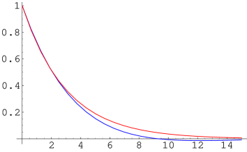
The first term vanishes because $\int_{0}^{\infty}{d\xi}\,\xi\,{\cal K}_{2}(\xi)=0$, and the leading term has $1/Q^{4}$ behavior. However, the next, $1/Q^{6}$, correction exceeds it for all $Q^{2}$ up to $12M^{2}\sim 7\,$  GeV², and the $1/Q^{4}$ asymptotics establishes somewhere above 20 GeV². Now, this fact is very welcome: due to it, the $F_{M}^{\rm spinor}(Q^{2})$ curve in the region of a few GeV² imitates the “power counting” $1/Q^{2}$ behavior much more successfully than Eq. (11) that displays its nominal $1/Q^{2}$ asymptotics only well outside the few GeV² region (see Fig. 3).

Figure 3: Meson form factors: $Q^{2}F_{M}(Q^{2})$ (upper curve, red online), $Q^{2}F_{M}^{\rm spinor}(Q^{2})$ (middle curve, green online); for comparison also shown $Q^{2}/(1+Q^{2}/m_{\rho}^{2})$ (lower curve, blue online).

The miraculous cancellation of the moments for $K_{2}(\xi)$ and $K_{3}(\xi)$ in (27) producing the $F_{M}^{\rm spinor}(Q^{2})\sim M^{4}/Q^{4}$ result can be traced to the $1/Q^{4}$ asymptotic behavior of the underlying double spectral density $\rho(s_{1},s_{2},Q^{2})$. To this end, consider the double Borel transform of the three-point function Ioffe:1982qb ; Nesterenko:1982gc

$$\Phi(\tau_{1},\tau_{2},Q^{2})=\frac{1}{\pi^{2}}\int_{0}^{\infty}ds_{1}\int_{0}^{\infty}ds_{2}\ \rho(s_{1},s_{2},Q^{2})\,e^{-s_{1}\tau_{1}-s_{2}\tau_{2}}\ ,$$ (28)

in which the power weights are substituted by the exponential ones. For the triangle diagram Nesterenko:1982gc ,

$$\Phi(\tau_{1},\tau_{2},Q^{2})=\frac{N_{c}}{2\pi^{2}(\tau_{1}+\tau_{2})}\int_{0}^{1}dx\,x\bar{x}\,\exp\left[-Q^{2}\frac{\bar{x}\,\tau_{1}\tau_{2}}{x(\tau_{1}+\tau_{2})}\right]\ .$$ (29)

It contains the $x\bar{x}$ factor (absent in the case of scalar quarks) that results in the $1/Q^{4}$ behavior of $\Phi(\tau_{1},\tau_{2},Q^{2})$ and, hence, of the spectral density $\rho(s_{1},s_{2},Q^{2})={N_{c}}\,\theta(s_{1})\,\theta(s_{2})\,(s_{1}+s_{2})/2Q^{4}+\ldots$  .

VI Local quark-hadron duality

Referring to the “established” $1/Q^{2}$ behavior of meson form factors at large $Q^{2}$, one primarily has in mind the data on the pion EM form factor which resemble the VMD monopole form $F_{\pi}(Q^{2})\sim 1/(1+Q^{2}/m_{\rho}^{2})$. In fact, the data are well described by our local quark-hadron duality model Nesterenko:1982gc that incorporates, in a simplified form, some ideas of Migdal’s program and the QCD sum rule approach Shifman:1978bx . From the latter, we borrow the observation that only the lowest state is narrow, and use the model spectrum: first resonance plus perturbative “continuum” starting from some effective scale $s=s_{0}$. In other words, we transform the two-current correlator $\Pi(p^{2})$ into

$$\Pi(p^{2})=\frac{1}{\pi}\int_{0}^{\infty}ds\,\frac{\rho^{\rm pert}(s)}{s-p^{2}}\Rightarrow\Pi^{\rm LD}(p^{2})=\frac{F_{M}^{2}}{M^{2}-p^{2}}+\frac{1}{\pi}\int_{s_{0}}^{\infty}\frac{\rho^{\rm pert}(s)}{s-p^{2}}\,ds\,.$$ (30)

Then we try to reach the best possible agreement between the original and model correlators in the deep spacelike region of $p^{2}\equiv-P^{2}$. For axial currents, $F_{M}\to f_{\pi}$, $M\to m_{\pi}\approx 0$, $\rho^{\rm pert}(s)=1/4\pi$, and

$$\Pi(p^{2})-\Pi^{\rm LD}(p^{2})=\frac{f_{\pi}^{2}}{p^{2}}+\frac{1}{4\pi^{2}}\int_{0}^{s_{0}}ds\,\frac{\rho^{\rm pert}(s)}{s-p^{2}}.$$ (31)

To eliminate the leading $1/p^{2}$ term in this difference, we should take $f_{\pi}^{2}=s_{0}/4\pi^{2}$. As a result, the coupling $f_{\pi}$ and the value of $s_{0}$ are connected by the local duality relation

$$\int_{0}^{s_{0}}\rho_{\pi}(s)\,ds=\int_{0}^{s_{0}}\rho^{\rm pert}(s)\,ds$$ (32)

between the spectral density $\rho_{\pi}(s)=\pi f_{\pi}^{2}\delta(s)$ of the lowest state and the perturbative spectral density $\rho^{\rm pert}(s)$, applied within the “duality interval” $s_{0}$. Transforming the $n^{\alpha}n^{\beta}n_{\mu}$ projection of the 3-point function

$${T}^{\rm pert}(p_{1}^{2},p_{2}^{2},Q^{2})\Rightarrow\frac{f_{\pi}^{2}\,F_{\pi}(Q^{2})}{p_{1}^{2}\,p_{2}^{2}}+\frac{1}{\pi^{2}}\int_{0}^{\infty}ds_{1}\int_{0}^{\infty}ds_{2}\ \Biggl{[}1-\theta(s_{1}\leq s_{0})\theta(s_{2}\leq s_{0})\Biggr{]}\,\frac{\rho^{\rm pert}(s_{1},s_{2},Q^{2})}{(s_{1}-p_{1}^{2})(s_{2}-p_{2}^{2})}\ ,$$ (33)

and requiring that the difference between $T^{\rm pert}(p_{1}^{2},p_{2}^{2},Q^{2})$ and the model function vanishes faster than $1/p_{1}^{2}p_{2}^{2}$ for large spacelike $p_{1}^{2},p_{2}^{2}$, gives the local duality relation for the pion form factor Nesterenko:1982gc

$$f_{\pi}^{2}F_{\pi}^{\rm LD}(Q^{2})=\frac{1}{\pi^{2}}\int_{0}^{s_{0}}ds_{1}\int_{0}^{s_{0}}ds_{2}\ \rho^{\rm pert}(s_{1},s_{2},Q^{2}).$$ (34)

Using Eq. (24) for $\rho^{\rm pert}(s_{1},s_{2},Q^{2})$ with $n(x)=6x\bar{x}$ and $f_{\pi}^{2}=s_{0}/4\pi^{2}$ produces the Drell-Yan formula

$$F_{\pi}^{\rm LD}(Q^{2})=\frac{6}{\pi s_{0}}\int_{0}^{1}\,dx\,\int d^{2}{\bf k}_{\perp}\,\theta\left({\bf k}_{\perp}^{2}\leq x\bar{x}s_{0}\right)\theta\left(({\bf k}_{\perp}+\bar{x}{\bf q}_{\perp})^{2}\leq x\bar{x}s_{0}\right)$$ (35)

with the effective “local duality wave function” $\widetilde{\Psi}^{\rm LD}_{\pi}(x,{\bf k}_{\perp})=\sqrt{{6}/{\pi s_{0}}}\ \theta({k}_{\perp}^{2}\leq x\bar{x}s_{0})$ for the pion. In the impact parameter representation, $\Psi^{\rm LD}_{\pi}(x,{\bf b}_{\perp})=\sqrt{{6x\bar{x}}/{\pi}}\,J_{1}(b\sqrt{x\bar{x}s_{0}})/b$. Taking the $b\to 0$ limit gives the model distribution amplitude $\varphi^{\rm LD}_{\pi}(x)=6f_{\pi}x\bar{x}$, that coincides with the asymptotic pion DA. Explicit expression for the pion form factor in the local duality model is known from Nesterenko:1982gc :

$$F_{\pi}^{\rm LD}(Q^{2})=1-\frac{1+{6s_{0}}/{Q^{2}}}{\left(1+{4s_{0}}/{Q^{2}}\right)^{3/2}}=\frac{6s_{0}^{2}}{Q^{4}}-\frac{40s_{0}^{3}}{Q^{6}}+\frac{210s_{0}^{4}}{Q^{8}}-\frac{1008s_{0}^{4}}{Q^{8}}+\ {\cal O}(s_{0}^{5}/Q^{10})\ .$$ (36)

As expected, $F_{\pi}^{\rm LD}(Q^{2})$ behaves like $1/Q^{4}$ for large $Q^{2}$, but the expansion parameter of this series is again large $\sim 6s_{0}/Q^{2}\approx 4$ GeV², so that the asymptotic $1/Q^{4}$ estimate should not be used at accessible $Q^{2}$. However, in the region of a few $Q^{2}$, the $F_{\pi}^{\rm LD}(Q^{2})$ curve successfully imitates the $1/Q^{2}$ behavior and goes very close to existing Volmer:2000ek and preliminary Horn:2006 experimental data.

         

Figure 4: “Holographized” local duality wave function $\sqrt{\pi s_{0}/6}\,\Psi^{\rm LD,holo}_{\pi}(x,{\bf k}_{\perp})$ vs. $k_{\perp}/\sqrt{x\bar{x}}$ in GeV.

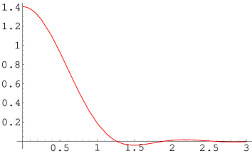
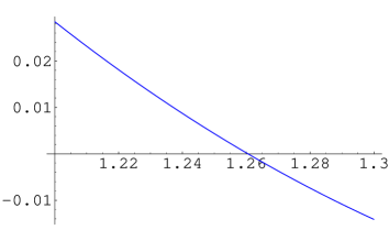
The sharp cut-off form of $\Psi^{\rm LD}_{\pi}(x,{\bf k}_{\perp})$ is a consequence of a simple model for the higher states’ contribution. The resulting $b$-space function $\Psi^{\rm LD}(x,{\bf b}_{\perp})$ has a Bessel-type form, but goes beyond the first zero. “Holographizing” it by imposing the cut-off $\theta(b\sqrt{x\bar{x}s_{0}}\leq\beta_{1,1})$, we found that its ${\bf k}_{\perp}$ version has a smooth dependence on ${k}_{\perp}^{2}/x\bar{x}$, qualitatively similar to that of Eq.(9), with the lowest zero located at ${k}_{\perp}^{2}/x\bar{x}\approx(1.26$ GeV$)^{2}$, i.e., “unexpectedly close” to the $A_{1}$ position (see Fig. 4).

VII Higher orders and transition to pQCD

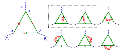
Both in the meromorphization and local duality approaches one can include higher order $\alpha_{s}$ corrections to spectral densities. In particular, the two-loop calculation of $\rho(s_{1},s_{2},Q^{2})$ for axial and vector currents was performed in Braguta:2004ck . Among ${\cal O}(\alpha_{s})$ contributions, there are gluon-exchange diagrams whose asymptotic large-$Q^{2}$ behavior is determined by the hard pQCD mechanism (see Fig. 5). As a result, the leading $1/Q^{2}$ term of the spectral density corresponding to the $T^{\mu}_{\alpha\beta}n_{\mu}n^{\alpha}n^{\beta}$ projection can be written in pQCD-like form,

$$\rho_{\alpha_{s}}(s_{1},s_{2},Q^{2})=2{\pi}{\alpha_{s}}\,\frac{C_{F}}{N_{c}}\int_{0}^{1}{dx}\,\int_{0}^{1}dy\ \frac{\rho(x,s_{1})\rho(y,s_{2})}{xyQ^{2}}\,+{\cal O}(1/Q^{4})\,,$$ (37)

where $\rho(x,s_{1})$ is the lowest order term for the $x$-unintegrated spectral density,

$$\rho(x,s_{1})=\frac{N_{c}}{2\pi^{2}}\int\delta\left(s_{1}-\frac{k_{1\perp}^{2}}{x\bar{x}}\right)\,d^{2}{\bf k}_{1\perp}=\frac{N_{c}}{2\pi}\,\theta(s_{1})\,x\bar{x}$$ (38)

(and similarly for $\rho(y,s_{2})$).

Figure 5: Diagrams producing spectral density $\rho(s_{1},s_{2},Q^{2})$ at the one-loop and two-loop (${\cal O}(\alpha_{s})$) level. Outlined diagrams are responsible for the leading pQCD $1/Q^{2}$ behavior.

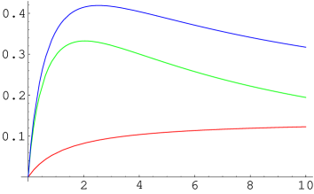
Integrating $\rho(x,s)$ over the duality interval $0\leq s\leq s_{0}$ and dividing result by $\pi f_{\pi}$ gives the local duality model $\varphi^{\rm LD}_{\pi}(x)=6f_{\pi}x\bar{x}=\varphi^{\rm as}_{\pi}(x)$ for the pion DA. Thus, substituting the ${\cal O}(1/Q^{2})$ part of $\rho_{\alpha_{s}}(s_{1},s_{2},Q^{2})$ into the local duality relation (34) gives the pQCD hard gluon exchange contribution $F_{\pi}^{\rm pQCD}(Q^{2})=8\pi\alpha_{s}f_{\pi}^{2}/Q^{2}$ calculated for the asymptotic shape of the pion DA. It is instructive to rewrite this result in the form $F_{\pi}^{\rm pQCD}(Q^{2})=2(s_{0}/Q^{2})(\alpha_{s}/\pi)$ that clearly reveals its nature as the $\alpha_{s}$ correction to the soft contribution (36), with the $(\alpha_{s}/\pi)$ factor being the standard penalty for an extra loop. Using full expressions for $\rho_{\alpha_{s}}(s_{1},s_{2},Q^{2})$ one can get the local duality model prediction for $F_{\pi}^{{\rm LD}(\alpha_{s})}$ at all $Q^{2}$, see Ref. Braguta:2004ck . In fact, a very good approximation is given by a simple interpolation formula $F_{\pi}^{{\rm LD}(\alpha_{s})}(Q^{2})=(\alpha_{s}/\pi)/(1+Q^{2}/2s_{0})$ Radyushkin:1990te between the $Q^{2}=0$ value $F_{\pi}^{{\rm LD}(\alpha_{s})}(0)=\alpha_{s}/\pi$ (that can be obtained, e.g., from the two-point result $\rho(s)=\theta(s)(1+\alpha_{s}/\pi)$ using the Ward identity) and the large-$Q^{2}$ asymptotic behavior. With $\alpha_{s}/\pi\approx 0.1$, the ${\cal O}(\alpha_{s})$ term is a $\lesssim 30\%$ correction to the ${\cal O}(\alpha_{s}^{0})$ term in the $Q^{2}\leq 4$  GeV² region (see Fig. 6), and their sum is in good agreement with existing data.

Figure 6: Pion form factor in local quark-hadron duality model: $Q^{2}F_{\pi}^{{\rm LD}(\alpha_{s})}$ (lower curve, red online), $Q^{2}F_{\pi}^{{\rm LD}}$ (middle curve, green online), total contribution (upper curve, blue online).

VIII Summary and conclusions

In this letter, we studied the large-$Q^{2}$ behavior of the meson form factor $F_{M}(Q^{2})$ constructed using the holographic model of Ref. Brodsky:2006uq , and observed that, despite its $1/Q^{2}$ asymptotic behavior, the combination $Q^{2}F_{M}(Q^{2})$ is not flat in the accessible region $Q^{2}\lesssim 10$  GeV². We also found that the asymptotic $1/Q^{2}$ result is governed by the Feynman mechanism rather than by large transverse momentum dynamics. We discussed the meromorphization approach, in which the form factors are given by integrating the perturbative spectral density $\rho(s_{1},s_{2},Q^{2})$ with weights proportional to $J_{0}(\beta_{0,1}\sqrt{s_{i}}/M)/(s_{i}-M^{2})$, and showed that, if one uses scalar currents made of scalar quarks, the result coincides with the expression given in Ref. Brodsky:2006uq . For spin-1/2 quarks, we studied a particular tensor projection of the 3-point function, and demonstrated that, due to an extra $(1-x)$ factor, the resulting form factor $F^{\rm spinor}_{M}(Q^{2})$ has $1/Q^{4}$ asymptotic behavior. However, owing to the late onset of this asymptotic pattern, the combination $Q^{2}F^{\rm spinor}_{M}(Q^{2})$ is rather flat in the phenomenologically important few GeV² region, i.e., $F^{\rm spinor}_{M}(Q^{2})$ imitates the $1/Q^{2}$ behavior. Then we presented the results for the pion form factor obtained in the local quark-hadron duality model, which corresponds to integrating the perturbative spectral density $\rho(s_{1},s_{2},Q^{2})$ with $\theta(s_{1}\leq s_{0})$ weights. Again, the lowest-order term has nominally the $1/Q^{4}$ asymptotics, but it imitates the $1/Q^{2}$ behavior in the few GeV² region. Including the ${\cal O}(\alpha_{s})$ correction term of $\rho(s_{1},s_{2},Q^{2})$ brings in the hard pQCD contribution having the dimensional counting $1/Q^{2}$ behavior at large $Q^{2}$. However, at accessible $Q^{2}$, the ${\cal O}(\alpha_{s})$ term is a rather small fraction of the total result, because of small $\alpha_{s}/\pi\sim 0.1$ factor associated with each higher order correction.

We did not discuss the nucleons form factors in the present paper, but we want to mention that the lowest-order perturbative density for spin-1/2 quarks is known Nesterenko:1982gc , and since the double Borel representation (see Eq.(29)) in that case has $(1-x)^{2}$ factor, the resulting asymptotic behavior of $\rho(s_{1},s_{2},Q^{2})$ is $1/Q^{6}$. But the local duality result for $G_{M}^{p}(Q^{2})$ closely follows the dipole shape of the data up to $Q^{2}\sim 15$  GeV².

Thus, we observe that the power of $(1-x)$ in these perturbative versions of the relevant parton densities $f(x)$ increases with the number of quarks like $f_{n}(x)\sim(1-x)^{n-1}$, i.e., the probability that the total momentum of $n-1$ spectators is $x_{\rm sp}$ goes like $x_{\rm sp}^{n-1}$, which looks quite natural. Due to Feynman mechanism, this formally gives $(1/Q^{2})^{n}$ behavior for form factors. However, because of the late onset of the asymptotic regime, the form factors imitate $(1/Q^{2})^{n-1}$ behavior in a rather wide preasymptotic region. In this scenario, the “observed” quark counting rules is an approximate and transitional phenomenon dominated by nonperturbative, long-distance aspects of hadron dynamics.

Acknowledgements. I thank S. J. Brodsky and G. de Teramond for correspondence, and H. Grigoryan for useful discussions.

Notice: This manuscript has been authored by Jefferson Science Associates, LLC under Contract No. DE-AC05-06OR23177 with the U.S. Department of Energy. The United States Government retains and the publisher, by accepting the article for publication, acknowledges that the United States Government retains a non-exclusive, paid-up, irrevocable, world-wide license to publish or reproduce the published form of this manuscript, or allow others to do so, for United States Government purposes.

References

- (1) V. A. Matveev, R. M. Muradian and A. N. Tavkhelidze, Lett. Nuovo Cimento 7, 719 (1973).
- (2) S. J. Brodsky and G. R. Farrar, Phys. Rev. Lett. 31, 1153 (1973).
- (3) D. R. Jackson, Ph. D. Thesis, Caltech (1977); G. R. Farrar and D. R. Jackson, Phys. Rev. Lett. 43, 246 (1979)
- (4) V. L. Chernyak, A. R. Zhitnitsky and V. G. Serbo, JETP Lett. 26, 594 (1977); Sov. J. Nucl. Phys. 31, 552 (1980)
- (5) A. V. Radyushkin, JINR report R2-10717 (1977), arXiv:hep-ph/0410276 (English translation); A. V. Efremov and A. V. Radyushkin, Theor. Math. Phys. 42, 97 (1980); Phys. Lett. B 94, 245 (1980)
- (6) G. P. Lepage and S. J. Brodsky, Phys. Lett. B 87, 359 (1979); Phys. Rev. Lett. 43, 545 (1979) [Erratum-ibid. 43, 1625 (1979)]; Phys. Rev. D 22, 2157 (1980)
- (7) A. V. Radyushkin, Phys. Rev. D 58, 114008 (1998)
- (8) A. V. Belitsky, X. d. Ji and F. Yuan, Phys. Rev. D 69, 074014 (2004)
- (9) M. Diehl, T. Feldmann, R. Jakob and P. Kroll, Eur. Phys. J. C 39, 1 (2005)
- (10) M. Guidal, M. V. Polyakov, A. V. Radyushkin and M. Vanderhaeghen, Phys. Rev. D 72, 054013 (2005)
- (11) R. P. Feynman, Photon-Hadron Interactions, Benjamin, New York (1972).
- (12) J. Polchinski and M. J. Strassler, JHEP 0305, 012 (2003)
- (13) S. J. Brodsky and G. F. de Teramond, Phys. Lett. B 582, 211 (2004)
- (14) S. J. Brodsky and G. F. de Teramond, Phys. Rev. Lett. 96, 201601 (2006)
- (15) S. D. Drell and T. M. Yan, Phys. Rev. Lett. 24, 181 (1970).
- (16) J. Erlich, G. D. Kribs and I. Low, Phys. Rev. D 73, 096001 (2006) [arXiv:hep-th/0602110].
- (17) A. A. Migdal, Annals Phys. 109, 365 (1977)
- (18) H. G. Dosch, J. Kripfganz and M. G. Schmidt, Phys. Lett. B 70, 337 (1977); Nuovo Cim. A 49, 151 (1979)
- (19) V. A. Nesterenko and A. V. Radyushkin, Phys. Lett. B 115, 410 (1982); Phys. Lett. B 128, 439 (1983)
- (20) D. E. Soper, Phys. Rev. D 15, 1141 (1977)
- (21) A. V. Radyushkin, Acta Phys. Polon. B 26, 2067 (1995) [arXiv:hep-ph/9511272].
- (22) G. P. Lepage, S. J. Brodsky, T. Huang and P. B. Mackenzie, In: Particles and Fields 2, Eds. A. Z. Capri and A. N. Kamal, Plenum Press, New York (1981).
- (23) A. Mukherjee, I. V. Musatov, H. C. Pauli and A. V. Radyushkin, Phys. Rev. D 67, 073014 (2003)
- (24) A. Karch, E. Katz, D. T. Son and M. A. Stephanov, arXiv:hep-ph/0602229.
- (25) A. Radyushkin, Annalen Phys. 13, 718 (2004) [arXiv:hep-ph/0410153].
- (26) B. L. Ioffe and A. V. Smilga, Nucl. Phys. B 216 373 (1983)
- (27) M. A. Shifman, A. I. Vainshtein and V. I. Zakharov, Nucl. Phys. B 147, 385 (1979)
- (28) J. Volmer et al. [The Jefferson Lab F(pi) Collaboration], Phys. Rev. Lett. 86, 1713 (2001)
- (29) T. Horn, Jefferson Lab seminar, April 2006.
- (30) V. V. Braguta and A. I. Onishchenko, Phys. Lett. B 591, 267 (2004) Phys. Rev. D 70, 033001 (2004)
- (31) A. V. Radyushkin, Nucl. Phys. A 532, 141 (1991)