1. It is well-known, that the renormalization procedure is ambiguous [1, 2]. Let for simplicity only the interaction constant $g$ is renormalized. Any observable quantity $A$, defined by a perturbation expansion, is a function $F(g_{0},\Lambda)$ of the bare value $g_{0}$ and the momentum cut-off $\Lambda$. According to the renormalization theory, $A$ becomes independent on $\Lambda$, if it is expressed in terms of renormalized $g$:

$$A=F(g_{0},\Lambda)=F_{R}(g)\,.$$

The renormalized coupling constant $g$ is usually defined in terms of a certain vertex, e.g. the four-leg vertex $\Gamma_{4}(p_{i},m)$ in the $g\phi^{4}$ theory, attributed to a certain length scale $L$ through some choice of mass $m$ and momenta $p_{i}$. Two types of definition are conventionally used:

(1) $m$ is finite, $p_{i}=0$, and $g=\Gamma_{4}(0,m)$ corresponds to a length scale $L\sim m^{-1}$;

(2) $m=0$, $p_{i}\sim\mu$, and $g=\Gamma_{4}(p_{i},0)$ corresponds to a length scale $L=\mu^{-1}$; the condition $p_{i}\sim\mu$ is technically realized by the equality

$$p_{i}\cdot p_{j}=a_{ij}\mu^{2}\,,$$

where $a_{ij}$ are usually taken for the so called ”symmetric point”, $a_{ij}=(4\delta_{ij}-1)/3$, though any other choice $a_{ij}\sim 1$ is possible.

Already the choice either (1) or (2) with different constants $a_{ij}$ provides essential ambiguity of the renormalization scheme. In fact, the physical condition that $g$ is determined by a vertex $\Gamma_{4}$ on the length scale $L$ can be realized technically in many variants (e.g. using averaging over $p_{i}$ with some weight function localized on the scale $L^{-1}$).

On the conceptual level, the change of the renormalization scheme is simply a change of variables,

$$g=f(\tilde{g})\,,$$

transforming (1) into equation

$$A=F(g_{0},\Lambda)=\tilde{F}_{R}(\tilde{g})$$

of the same form. Such change of variables does not affect values of observable quantities but changes a specific form of functions $F_{R}(g)$.

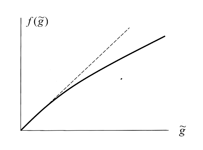
In the lowest order of the perturbation expansion, the equality $\Gamma_{4}=g_{0}$ takes place independently of $p_{i}$ and $m$, and one have the first physical restriction for the function $f(\tilde{g})$:

$\qquad(R_{1})\qquad\qquad\qquad\qquad\qquad f(\tilde{g})=\tilde{g}+O(\tilde{g}^{2})\,.$

In fact, the analogous condition $f(\tilde{g})\sim\tilde{g}$ should be valid in the order of magnitude in the large $\tilde{g}$ region, so as to $\tilde{g}$ has the same physical sense, as $g$ (if for example $f(\tilde{g})\sim\tilde{g}^{2}$, then $\tilde{g}$ corresponds to $\left(\Gamma_{4}\right)^{1/2}$ instead $\Gamma_{4}$). Consequently, the difference between the conventional renormalization schemes corresponds to a change of variables (2) with a function $f(\tilde{g})$ of appearance shown in Fig.1.

Figure 1:

2. If we apply a change of variables (2) to the Gell-Mann – Low equation 

$$-\frac{dg}{d\ln L}=\beta(g)=\beta_{2}g^{2}+\beta_{3}g^{3}+\beta_{4}g^{4}+\ldots\,,$$

then it transforms to

$$-\frac{d\tilde{g}}{d\ln L}=\tilde{\beta}(\tilde{g}),\qquad{\rm where}\qquad\tilde{\beta}(\tilde{g})=\beta(f(\tilde{g}))/f^{\prime}(\tilde{g})\,.$$

It is easy to be convinced that the restriction $(R_{1})$ provides invariance of two coefficients $\beta_{2}$ and $\beta_{3}$ under the change of the renormalization scheme.

In 1977 ’t Hooft has suggested [4] to fix the renormalization scheme by the condition, that Eq.5 has exactly the two-loop form

$$-\frac{d\tilde{g}}{d\ln L}=\beta_{2}\tilde{g}^{2}+\beta_{3}\tilde{g}^{3}\,.$$

In the framework of perturbation theory it is always possible: if

$$g=f(\tilde{g})=\tilde{g}+\alpha_{1}\tilde{g}^{2}+\alpha_{2}\tilde{g}^{3}+\alpha_{3}\tilde{g}^{4}+\ldots\,,$$

then (5) has a form

$$-\frac{d\tilde{g}}{d\ln L}=\beta_{2}\tilde{g}^{2}+\beta_{3}\tilde{g}^{3}+(-\alpha_{2}\beta_{2}+\beta_{4})\tilde{g}^{4}+(-2\alpha_{3}\beta_{2}+\beta_{5})\tilde{g}^{5}+\ldots$$

The parameter $\alpha_{1}$ can be fixed arbitrarily and we accepted $\alpha_{1}=0$ for simplicity. The coefficient $\alpha_{n}$ appears for the first time in the term of the order $\tilde{g}^{n+2}$ and choosing successively

$$\alpha_{2}=\frac{\beta_{4}}{\beta_{2}}\,,\qquad\alpha_{3}=\frac{\beta_{5}}{2\beta_{2}}\,,\quad\ldots$$

one can eliminate the terms $\tilde{g}^{4}$, $\tilde{g}^{5}\,\ldots$ in the r.h.s. of (8). If this construction can be used beyond perturbation context, it provides a powerful instrument for investigation of general aspects of theory.

3. From the physical viewpoint, the choice of $f(\tilde{g})$ is strongly restricted (Fig.1), but formally one can choose this function rather arbitrary. Nevertheless, there is a minimal physical restriction that should be added to $(R_{1})$:

$(R_{2})\qquad$ $f(\tilde{g})$ should be regular and provide one to one correspondence between $\phantom{vvvvvvvvvvv}g$ and $\tilde{g}$, at least for their physical values, $g,\tilde{g}\in(0,\infty)$

Indeed, variation of $g$ from $0$ to $\infty$ should correspond to variation  of $\tilde{g}$ from $0$ to $\infty$, and this change of variables should not create artificial singularities in the theory. It should be stressed, that $(R_{2})$ is not controlled in the above construction, where $f(\tilde{g})$ is defined by a formal series in $\tilde{g}$. It is easy to demonstrate, that restriction $(R_{2})$ forbides to use ’t Hooft’s construction beyond perturbation theory.

According to classification by Bogolyubov and Shirkov [1], there are three possible types of the $\beta$-function, corresponding to three qualitatively different situations for the dependence of $g$ on the length scale $L$. For $\beta_{2}>0$ they are:

(a) $\beta(g)$ has a nontrivial zero $g_{c}$; then $g(L)\to g_{c}$ for $L\to 0$.

(b) $\beta(g)$ is nonalternating and behaves as $g^{\alpha}$ with $\alpha\leq 1$ for $g\to\infty$; then $g(L)\to\infty$ for $L\to 0$.

(c) $\beta(g)$ is nonalternating and behaves as $g^{\alpha}$ with $\alpha>1$ for $g\to\infty$; then $g(L)\to\infty$ at some finite point $L_{0}$ (Landau pole) and the dependence $g(L)$ is not defined for $L<L_{0}$, signalling that the theory is internally inconsistent (or trivial).

In the case $\beta_{2}<0$, the same conclusions hold for the limit $L\to\infty$ instead of $L\to 0$.

It is easy to see, that the restriction $(R_{2})$ forbids to transform one of the situations (a), (b), (c) into another. Let $\tilde{g}$ corresponds to (a) or (b), and $g$ corresponds to (c): then $g$ goes to infinity at the point $L=L_{0}$, where $\tilde{g}$ has a finite value $g^{*}$. Consequently, $f(\tilde{g})\to\infty$ for $\tilde{g}\to g^{*}$ and regularity of $f(\tilde{g})$ is violated; more than that, $f(\tilde{g})$ is not defined for $\tilde{g}>g^{*}$ (Fig.2,a). Analogously, if $g$ corresponds to (b) and $\tilde{g}$ corresponds to (a), then $g\to\infty$ and $\tilde{g}\to g_{c}$ in the small $L$ limit; so $f(\tilde{g})\to\infty$ for $\tilde{g}\to g_{c}$ and $f(\tilde{g})$ is not regular, while its inverse is double-valued (Fig. 2,b). We see, that classification by Bogolyubov and Shirkov has an absolute character and cannot be smashed by the change of the renormalization scheme.

Figure 2:

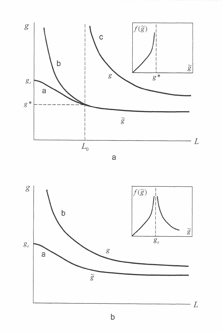
When ’t Hooft’s form (6) is postulated, a situation (b) becomes impossible from the very beginning. The choice between other two situations is also made, when the known coefficients $\beta_{2}$ and $\beta_{3}$ are taken into account. Consequently, the type of the field theory is fixed, using the knowledge of only two expansion coefficients, but that is surely unjustifiable. It easy to see, that ’t Hooft’s construction predetermines internal inconsistency for QED ($\beta_{2}>0$, $\beta_{3}>0$) and QCD ($\beta_{2}<0$, $\beta_{3}<0$), and the fixed-point situation (a) for the $\phi^{4}$ theory ($\beta_{2}>0$, $\beta_{3}<0$).

It is commonly accepted that there no effective way beyond perturbative theory. In fact, such way does exist. One can calculate few first expansion coefficients diagrammatically and their large-order asymptotics in the framework of the instanton method suggested by Lipatov [5]; producing the smooth interpolation for the coefficient function, one can find the sum of the whole perturbation series. Such program was realized in [6, 7, 8] for reconstruction of the $\beta$-fuctions for the main field theories (see also the review article [9]). The results have reasonable uncertainty and suggest a situation (b) for the $\phi^{4}$ theory [6] and QED [7], while situations (a) and (b) are possible for QCD [8]. All these results are in conflict with ’t Hooft’s construction. Of course, one can have a reasonable doubt that existing information is sufficient for reliable reconstruction of the $\beta$-functions, but the results of [6, 7, 8] are certainly more reliable, than an arbitrary choice made in the ’t Hooft scheme. In the case of the $\phi^{4}$ theory, there is some controversy concerning the asymptotics of the $\beta$-function [6, 10, 11, 12], but there is a consensus that the $\beta$-function is not alternating. The same conclusion follows from the lattice results [13] and the real-space renormalization group analysis [14].  As for QCD, it looks as successful theory of strong interactions and hardly deserves a status of internally inconsistent theory.

According to ’t Hooft, an arbitrary $\beta$–function can be reduced to the form (6). It creates an illusion that the physical $\beta$–function is not interesting quantity. In fact, the latter has the fundamental significance, allowing to distinguish three qualitatively different types (a),(b),(c) of field theory. This question is not pure academic. For example, the conventional bound on the Higgs mass is based on the expected triviality of the $\phi^{4}$ theory [15] and appears completely wrong, if it is not trivial. The latter looks rather probable, according to [6].

4. In fact, singularity of $f(\tilde{g})$ in the complex plane is evident from the very beginning. It is clear from the Dyson type arguments [16] and instanton calculations [5] that perturbation series for $\beta(g)$ is factorially divergent and $g=0$ is essential singularity; in fact, it is a branching point and all quantities have at least two leafs of the Riemann surface. In the ’t Hooft scheme, $\beta$-function is polynomial and does not possess the correct analytic properties.

5. As immediate application of his scheme, ’t Hooft derived accumulation of singularities for the Green functions near the origin $g=0$. He used the fact that momentum $k$ enters all quantities in combination $1/g+\beta_{2}\ln(k^{2}/\mu^{2})$. On the physical grounds, Green functions contain singularities for $g>0$, $k^{2}<0$, while for $k^{2}>0$ one expect singularities at the points

$$\frac{1}{g}=real+\beta_{2}(2n+1)\pi i\,\qquad n=0,\pm 1,\pm 2,\ldots.$$

Existence of such singularities has fundamental significance, since strong Borel summability of perturbative expansions becomes impossible.

Attempt to generalize this conclusion to the arbirary renormalization scheme was made by Khuri [17]. His analysis is based on expected regularity of the function $g=f(\tilde{g})$, relating ’t Hooft’s and some other scheme, in a certain sector of the complex plane. However, in proving this regularity Khuri discarded (as improbable) the case when $\beta(g)$ has an infinite set of zeroes accumulating near the origin. In fact, this case is not improbable. Consider the simplest (zero-dimensional) version of the functional integral entering the $\phi^{4}$ theory

$$F(g)=\int\limits_{-\infty}^{\infty}d\phi\,{\rm e}^{-\phi^{2}-g\phi^{4}}={\textstyle\frac{1}{2}}\,g^{-1/2}\,{\rm e}^{1/8g}\,K_{1/4}\left(\textstyle\frac{1}{8g}\right)$$

Its relation with the Mac-Donald function $K_{\nu}(x)$ can be established by observation that $F(g)$ satisfies an equation [18]

$$4g^{2}F^{\prime\prime}+(8g+1)F^{\prime}+{\textstyle\frac{3}{4}}F=0$$

with the boundary condition $F(0)=\sqrt{\pi}$. It is easy to show that the Mac-Donald function $K_{\nu}(z)$ has not zeroes on the main leaf of the Riemann surface, but has zeroes on the neighbouring leafs; for large $|z|$ they are 

$$z_{s}=-{\textstyle\frac{1}{2}}\ln(2\cos{\pi\nu})+{\rm e}^{\pm 3\pi i/2}\left({\textstyle\frac{3\pi}{4}}+\pi s\right)\,,\qquad s\,-\,integer$$

One can see from (11) that zeroes (13) correspond to the points of kind (10) in the complex $g$ plane. It is typical for functional integrals to have zeroes in such points and it is not miraculous if $\beta(g)$ has also such zeroes.

Then, according to Khuri’s analysis, the function $g=f(\tilde{g})$ is badly singular and has infinite number of singularities in the points of type (10); hence, one cannot be sure, are ’t Hooft’s singularities (10) of physical relevance or they are created by the singular transformation $g=f(\tilde{g})$.

One can come to the problem from another side. Zeroes of functional integrals correspond to poles in the Green functions (which are determined by ratios of such integrals), and hence their singularities are indeed of type (10). However (!) they lie on unphysical leaf of the Riemann surface. The choice of the leaf was not controlled in ’t Hooft’s considerations, since his scheme does not reproduce the correct analytic properties (Sec.4); in fact, such choice is not trivial since the Stokes phenomenon is intrinsic for functional integrals.

Regularity of the Green functions on the physical leaf can be easily shown, if one accept that their Borel transforms have the power-like behavior at infinity and suggest that $\beta(g)\sim g^{\alpha}$, $\alpha\leq 1$, for large $g$ [19]. Such assumptions look rather realistic according to [6, 7, 8].

We see that conclusion on accumulation of singularities following from the ’t Hooft scheme appears to be misleading: such singularities may either be absent or lie on unphysical leaf.

6. Another related aspect is the problem of renormalon singularities in the Borel plane [4, 20]. According to the recent analysis [19], existence or absence of such singularities is related with the analytic properties of the $\beta$-function. Briefly, results are as follows:

(i) Renormalon singularities are absent, if $\beta(g)$ has a proper behavior at infinity, $\beta(g)\sim g^{\alpha}$ with $\alpha\leq 1$, and its singularities at finite points $g_{c}$ are sufficiently weak, so that $1/\beta(g)$ is not integrable at $g_{c}$ (i.e. $\beta(g)\sim(g-g_{c})^{\gamma}$ with $\gamma\geq 1$).

(ii) Renormalon singularities exist, if at least one condition named in (i) is violated.

It is easy to see, that ’t Hooft’s form (6) corresponds to the behavior $\beta(g)\sim g^{3}$ at infinity and automatically creates renormalon singularities, even if they were absent in the physical renormalization scheme. It makes the field theory to be ill-defined due to impossibility of the proper definition of functional integrals. Indeed, the classical definition of the functional integral via the perturbation theory is defective due to non-Borel-summability of the perturbative series, while the lattice definition is doubtful due to restriction of large momenta, which are responsible for renormalon contributions [9, 19]. Contrary, the results of [6, 7, 8] show the possibility of self-consistent elimination of renormalon singularities and formulation of the well-defined field theory without renormalons [9, 19].

———————————-

In conclusion, the ’t Hooft representation for the $\beta$-function (6) is generally in conflict with the natural physical requirements and specifies the type of the field theory in an arbitrary manner. It violates analytic properties in the complex $g$ plane and provokes misleading conclusion on accumulation of singularities near the origin. It artificially creates renormalon singularities, even if they are absent in the physical scheme. The ’t Hooft scheme can be used in the framework of perturbation theory but no global conclusions should be drawn from it.

Author is indebted to participants of the PNPI Winter school for stimulating discussions, and to F.V.Tkachov and A.L.Kataev for consultations on the MS scheme.

References

- [1] N. N. Bogolyubov, D. V. Shirkov, Introduction to the Theory of Quatized Fields (Nauka, Moscow, 1976; Wiley, New York, 1980).
- [2] A. A. Vladimirov, D. V. Shirkov, Usp. Fiz. Nauk 129, 407 (1979) [Sov. Phys. Usp. 22, 860 (1979)].
- [3] A. A. Slavnov, L. D. Faddeev. Introduction to Quantum Theory of Gauge Fields (Nauka, Moscow, 1988).
- [4] ’t Hooft G., in: The whys of subnuclear physics (Erice, 1977), ed. A.Zichichi, Plenum Press, New York, 1979.
- [5] L. N. Lipatov, Zh. Eksp. Teor. Fiz. 72, 411 (1977) [Sov. Phys. JETP 45, 216 (1977)].
- [6] I. M. Suslov, Zh. Eksp. Teor. Fiz. 120, 5 (2001) [JETP 93, 1 (2001)]; hep-ph/0111231.
- [7] I. M. Suslov, Pis’ma Zh. Eksp. Teor. Fiz. 74, 211 (2001) [JETP Lett. 74, 191 (2001)]; hep-ph/0210239.
- [8] I. M. Suslov, Pis’ma Zh. Eksp. Teor. Fiz. 76, 387 (2002) [JETP Lett. 76, 327 (2002)]; hep-ph/0210439.
- [9] I. M. Suslov, Zh. Eksp. Teor. Fiz. 127, 1350 (2005) [JETP 100, 1188 (2005)]; hep-ph/0510142.
- [10] D. I. Kazakov, O. V. Tarasov, D. V. Shirkov, Teor. Mat. Fiz. 38, 15 (1979).
- [11] Yu. A. Kubyshin, Teor. Mat. Fiz. 58, 137 (1984).
- [12] A. N. Sissakian, I. L. Solovtsov, O. P. Solovtsova, Phys. Lett. B 321, 381 (1994).
- [13] B. Freedman, P. Smolensky, D. Weingarten, Phys. Lett. B 113, 481 (1982). I. A. Fox, I. G. Halliday, Phys. Lett. B 159, 148 (1985). M. G. do Amaral, R. C. Shellard, Phys. Lett. B 171, 285 (1986).
- [14] K. Wilson, J. B. Kogut, Phys. Rep. C 12, 75 (1974). D. J. E. Callaway, R. Petronzio, Nucl. Phys. B 240[FS12], 577 (1984). C. B. Lang, Nucl. Phys. B 265[FS15], 630 (1986).
- [15] J. Zinn-Justin, Phys. Rept. 385, 69 (2003).
- [16] F. J. Dyson, Phys.Rev. 85, 631 (1952).
- [17] N. N. Khuri, Phys.Rev. D 23, 2285 (1981).
- [18] D. I. Kazakov, Theor. Math. Phys. 46, 227 (1981).
- [19] I. M. Suslov, Zh. Eksp. Teor. Fiz. 126, 542 (2004) [JETP 99, 474 (2004)]; hep-ph/0510033.
- [20] M. Beneke, Phys. Rept. 317, 1 (1999).