Small $x$ Phenomenology - summary of the 3rd Lund Small $x$ Workshop in 2004

Abstract

A third workshop on small-$x$ physics, within the Small-x Collaboration, was held in Hamburg in May 2004 with the aim of overviewing recent theoretical progress in this area and summarizing the experimental status.

1 Introduction

In this report we summarize some of the recent developments in small-$x$ physics, based on presentations and discussions during the Lund Small-x workshop held in DESY, Hamburg in May 2004.

Although accepted as an integral part of the Standard Model, QCD is still not a completely understood theory. The qualitative aspects of asymptotic freedom and confinement are under control, but the quantitative predictive power of the theory is not at a satisfactory level. In particular this is true for the non-perturbative regime, where most of our understanding comes from phenomenological models, such as the Lund string fragmentation model, and also from lattice gauge calculations and effective theories, such as chiral perturbation theory. For the perturbative aspects of QCD, the situation is more satisfactory. In the weak coupling limit, the collinear factorization theorem with so-called DGLAP evolutionGribov:1972ri ; Lipatov:1975qm ; Altarelli:1977zs ; Dokshitzer:1977sg is working well and is under good theoretical control. Many cross sections have been calculated to next-to-leading order (NLO), several even to next-to-next-to-leading order, and some calculations involving (next-to)³-leading order have begun (see e.g. Moch:2004sf and references therein). The quantitative precision in this regime is approaching the per-mille level, which is very encouraging although still very far from the precision in QED.

However, there is a domain, still in the perturbative regime, where our understanding is lacking. This is the region of high energy and moderate momentum transfer, such as small-$x$ Deeply Inelastic Scattering (DIS) as measured at HERA and low to medium $E_{\perp}$ jet production at the Tevatron. In this region, the collinear factorization must break down as the perturbative expansion becomes plagued by large logarithms of the ratio between the total collision energy and the momentum transfer of the hard sub-process, which needs to be resummed to all orders to obtain precision predictions from QCD. These logarithms arise from the large increase of the phase space available for additional gluon emissions, resulting in a rapid rise of the gluon density in hadrons with increasing collision energy or, equivalently, decreasing momentum fraction, $x$.

In this high energy limit, QCD is believed to be correctly approximated by the BFKL evolutionKuraev:1976ge ; Kuraev:1977fs ; Balitsky:1978ic , and cross sections should be possible to predict using $k_{\perp}$-factorization Gribov:1984tu ; Levin:1991ry ; Catani:1991eg ; Collins:1991ty where off-shell matrix elements are convoluted with unintegrated parton densities obeying BFKL evolution. However, so far the precision in the predictions from $k_{\perp}$-factorization has been very poor. Although BFKL evolution correctly predicted the strong rise of the $F_{2}$ structure function with decreasing $x$ at HERA on a qualitative level, it turned out that the next-to-leading order corrections to BFKL are hugeFadin:1998py ; Ciafaloni:1998gs , basically making any calculation with leading-logarithmic accuracy in $k_{\perp}$-factorization useless.

Several attempts have been made to tame the NLO corrections to BFKL by e.g. matching to the collinear limitCiafaloni:1999yw and matching this with off-shell matrix elements or impact factors calculated to NLO. Another strategy is based on the fact that a large part of the NLO corrections to BFKL can be traced to the lack of energy and momentum conservation in the LO evolutionSalam:1999cn . Although energy and momentum is still not conserved in NLO evolution, the contributions from ladders which violates energy–momentum conservations are reduced. Amending the leading-logarithmic evolution with kinematical constraints, either approximately in analytical calculationsKwiecinski:1996td or exactly in Monte-Carlo programsOrr:1997im ; Kharraziha:1998dn ; Jung:2001hx ; Andersen:2003gs , should possibly lead to more reasonable QCD predictions, although still formally only to leading logarithmic accuracy. However, so far none of these strategies have been able to fulfill their ambitions, and the reproduction of available data is still not satisfactory.

The plot thickens further when considering the increase in gluon density at small $x$. At high enough energy the density of gluons becomes so high that they must start to overlap and recombine, and we will encounter the phenomena of multiple interactions, saturation and rapidity gaps. In the non-perturbative region these phenomena have already been established, but there is currently no consensus on whether effects of recombination of perturbative gluons have been seen at e.g. HERA. Perturbative recombination would require non-linear evolution equations, which then also could break $k_{\perp}$-factorization.

In our first review Andersson:2002cf we focused on the theoretical and phenomenological aspects of $k_{\perp}$-factorization, while in the second Andersen:2003xj we also gave an overview of experimental results in the small-$x$ region. In this third review we will continue to present recent developments in these areas, but also give an overview and introduction to saturation effects and non-linear evolution.

The layout of this report is as follows. First we discuss some recent developments of $k_{\perp}$-factorization in section 2, starting with the unintegrated parton densities (section 2.2) and doubly unintegrated parton densities (2.3) and continuing with recent advances in NLO calculations (2.4 and 2.6). Then, in section 3 we describe some phenomenological applications of $k_{\perp}$-factorization, looking at how to use them to obtain QCD predictions for heavy quark (3.1) and quarkonium (3.4) production. In section 4 we present the recent investigations by Marchesini and Mueller relating some aspects of jet physics to BFKL dynamics, which could make it possible to study this kind of evolution also in other environments. In section 5 we give an introduction and overview of saturation phenomena and non-linear evolution. Section 6 also deals with saturation, but in the context of the so-called AGK cutting rules which enables us to relate saturation with multiple scatterings and diffraction. In section 7 we review some recent experimental results relating to the issues in the previous sections, beginning with multiple interactions and underlying events in section 7.1, followed by rapidity gaps between jets in 7.2, jet-production at small-$x$ in 7.3 and production of strange particles in DIS in section 7.4. Finally we present a brief summary and outlook in section 8.

2 The $k_{\perp}$-factorization formalism

Main author H. Jung

In the high energy limit, cross sections can be calculated using $k_{\perp}$ -factorization Gribov:1984tu ; Levin:1991ry ; Catani:1991eg ; Collins:1991ty with convolution of a off-shell ($k_{\perp}$ dependent) partonic cross section $\hat{\sigma}(\frac{x}{z},k_{\perp}^{2})$ and an $k_{\perp}$ - unintegrated parton density function ${\cal F}(z,k_{\perp}^{2})$:

$$\sigma=\int\frac{dz}{z}d^{2}k_{\perp}\hat{\sigma}(\frac{x}{z},k_{\perp}^{2}){\cal F}(z,k_{\perp}^{2})$$ (1)

The unintegrated gluon density ${\cal F}(z,k_{\perp}^{2})$ is described by the BFKL Kuraev:1976ge ; Kuraev:1977fs ; Balitsky:1978ic evolution equation in the region of asymptotically large energies (small $x$). An appropriate description valid for both small and large $x$ is given by the CCFM evolution equation Ciafaloni:1988ur ; Catani:1990yc ; Catani:1990sg ; Marchesini:1994wr , resulting in an unintegrated gluon density, ${\cal A}(x,k_{\perp}^{2},\bar{q}^{2})$, which is a function also of the additional scale, $\bar{q}$. Here and in the following we use the following classification scheme: $x{\cal G}(x,k_{\perp}^{2})$ describes DGLAP type unintegrated gluon distributions, $x{\cal F}(x,k_{\perp}^{2})$ is used for pure BFKL and $x{\cal A}(x,k_{\perp}^{2},\bar{q}^{2})$ stands for a CCFM type or any other type having two scales involved. Different approaches to the unintegrated parton density functions have been discussed in detail in Andersson:2002cf ; Andersen:2003xj .

While still being formally at leading order, the unintegrated gluon densities incorporate effects from the next-to-leading order in the collinear approach Ryskin:2000bz . This is discussed in more detail in the next subsections. To further connect to the uncertainty estimates of cross section calculated in the collinear approach, the change of the renormalization and factorization scales are used to estimate the influence and size of higher order corrections. In Jung:2004gs the CCFM unintegrated PDFs are determined such that the structure function $F_{2}$ as measured at H1 Aid:1996au ; Adloff:2000qk and ZEUS Derrick:1996hn ; Chekanov:2001qu can be described after convolution with the off-shell matrix element. This fit is repeated for the renormalization scale in the off-shell matrix element varied by a factor of 2 up and down, resulting in new sets of PDFsJung:2004gs , set A0+ and set A0-. These PDFs are compared with the central set set A0 in Fig. 1.

Figure 1: Comparison of the CCFM uPDF obtained after changing the renormalization scale in the off-shell matrix element by a factor 2 up and down.

2.1 Future fits of uPDF parameterizations

Main author M. Hansson

There are a number of possible measurements sensitive to the transverse momentum of the propagating gluons in the gluon ladder, and thereby suitable for investigations concerning the unintegrated gluon density of the proton. One possible observable is the difference in azimuthal angle, $\Delta\phi^{\star}$, of a dijet system in the hadronic center of mass frame. The differential cross section $\frac{d\sigma}{d\Delta\phi^{\star}}$ has been measured at the Tevatron Acosta:2004nj ; Abazov:2004hm ; Abbott:1999se ; Abe:1995mj ; Abe:1996zt ; Acosta:2003nn and only recently at HERA Chekanov:2005zg ; Flucke:2005ux . The quantity

$$S=\frac{\int_{0}^{\alpha}N_{dijet}(\Delta\phi^{\star},x,Q^{2})d\Delta\phi^{\star}}{\int_{0}^{\pi}N_{dijet}(\Delta\phi^{\star},x,Q^{2})d\Delta\phi^{\star}},$$ (2)

first proposed in Szczurek:2000pj , has been measured Aktas:2003ja and showed a large sensitivity to the unintegrated gluon density. Another measurement, proposed in Luszczak:2004ag , would be to measure $\frac{d\sigma}{dp_{1,t}^{2}dp_{2,t}^{2}}$ where $dp_{i,t}^{2}$ are the transverse momenta of a charm anti-charm pair. In Luszczak:2004ag , also an alternative to this was discussed, namely to measure the quantity

$$f(p_{\max}^{2}>kp_{\min}^{2};W)\equiv\frac{\sigma(p_{\max}^{2}>kp_{\min}^{2};W)}{\sigma(W)}$$ (3)

where $p_{\max}^{2}=\max(dp_{1,t}^{2},dp_{2,t}^{2})$, $p_{\min}^{2}=\min(dp_{1,t}^{2},dp_{2,t}^{2})$ and $k$ is a constant. This quantity would be a measure of the spread in the $p_{1,t}^{2}\times p_{2,t}^{2}$ plane. Yet another possibility would be a direct reconstruction of $x_{g}$ and $k_{g,t}^{2}$ from (DIS) multijet events, thereby mapping the unintegrated gluon density directly.

The unintegrated gluon density could also be constrained from global fits. So far, only fits to $F_{2}$ have been made Hansson:2003xz , and a global fit using various data such as forward jets, 2+n jets, heavy quarks and azimuthal jet-jet correlations would further constrain the unintegrated gluon density.

2.2 The need for doubly unintegrated parton density functions

Main author J. Collins

Conventional parton densities are defined in terms of an integral over all transverse momentum and virtuality for a parton that initiates a hard scattering. While such a definition of an integrated parton density is appropriate for very inclusive quantities, such as the ordinary structure functions $F_{1}$ and $F_{2}$ in DIS, the definition becomes increasingly unsuitable as one studies less inclusive cross sections. Associated with the use of integrated parton densities are approximations on parton kinematics that can readily lead to unphysical cross sections when enough details of the final state are investigated.

We propose that it is important to the future use of pQCD that a systematic program be undertaken to reformulate factorization results in terms of fully unintegrated densities, which are differential in both transverse momentum and virtuality. These densities are called “doubly unintegrated parton densities” by Watt, Martin and Ryskin Watt:2003mx ; Watt:2003vf (discussed in the next section), and “parton correlation functions” by Collins and Zu Collins:2004vq ; these authors have presented the reasoning for the inadequacy, in different contexts, of the more conventional approach. The new methods have their motivation in contexts such as Monte-Carlo event generators where final-state kinematics are studied in detail. Even so, a systematic reformulation for other processes to use unintegrated densities would present a unified methodology.

Figure 2: (a) and (b): Comparison between use of simple LO parton model approximation and of the use of $k_{\perp}$ densities for the $p_{\perp}$ of $c\bar{c}$ pairs in photoproduction, and for the $x_{\gamma}$. (c) and (d): Comparison of use of $k_{\perp}$ densities and full simulation.

These methods form an extension of $k_{\perp}$-factorization, which has so far been applied in small-$x$ processes and, as the CSS formalismCollins:1984kg , in the transverse-momentum distribution of the Drell-Yan and related processes.

The problem that is addressed is nicely illustrated by considering photoproduction of $c\bar{c}$ pairs. In Figs. 2, we compare three methods of calculation carried out within the Cascade event generator Jung:2000hk ; Jung:2001hx :

• Use of a conventional gluon density that is a function of parton $x$ alone.

• Use of a $k_{\perp}$ density that is a function of parton $x$ and $k_{\perp}$. These are the objects usually called “unintegrated parton densities”.

• Use of a “doubly unintegrated density” that is a function of parton $x$, $k_{\perp}$ and virtuality, that is, of the complete parton 4-momentum, in Cascade taken after the full simulation of the initial state parton showering.

The partonic subprocess in all cases is the lowest order photon-gluon-fusion process $\gamma+g\longrightarrow c+\bar{c}$. Two differential cross sections are plotted: one as a function of the transverse momentum of the $c\bar{c}$ pair, and the other as a function of the $x_{\gamma}$ of the pair. By $x_{\gamma}$ is meant the fractional momentum of the photon carried by the $c\bar{c}$ pair, calculated in the light-front sense as

$$x_{\gamma}=\frac{\sum_{i=c,\bar{c}}(E_{i}-p_{z\;i})}{2yE_{e}}=\frac{p_{c\bar{c}}^{-}}{q^{-}}.$$

Here $E_{e}$ is the electron beam energy and the coordinates are oriented so that the electron and proton beams are in the $-z$ and $+z$ directions respectively.

In the normal parton model approximation for the hard scattering, the gluon is assigned zero transverse momentum and virtuality, so that the cross section is restricted to $p_{Tc\bar{c}}=0$ and $x_{\gamma}=1$, as shown by the solid lines in Fig. 2(a,b). When a $k_{\perp}$ dependent gluon density is used, quite large gluonic $k_{\perp}$ can be generated, so that the $p_{Tc\bar{c}}$ distribution is spread out in a much more physical way, as given by the dashed line in Fig. 2(a). But as shown in plot (b), $x_{\gamma}$ stays close to unity. Neglecting the full recoil mass $m$ is equivalent of taking $k^{2}=\frac{-k_{\perp}^{2}}{1-x}$ with $k^{2}$ being the virtuality of the gluon, $k_{\perp}^{2}$ its transverse momentum and $x$ its light cone energy fraction. This gives a particular value to the gluon’s $k^{-}$. When we also take into account the correct virtuality of the gluon, there is no noticeable change in the $p_{Tc\bar{c}}$ distribution — see Fig. 2(c) (dotted line) — since that is already made broad by the transverse momentum of the gluon. But the gluon’s $k^{-}$ is able to spread out the $x_{\gamma}$ distribution, as in Fig. 2(d) with the dotted line. This is equivalent with a proper treatment of the kinematics and results in $k^{2}=\frac{-k_{\perp}^{2}-xm^{2}}{1-x}$, which can be significant for finite $x$. Clearly, the use of the simple parton-model kinematic approximation gives unphysically narrow distributions. The correct physical situation is that the gluon surely has a distribution in transverse momentum and virtuality, and for the considered cross sections neglect of parton transverse momentum and virtuality leads to wrong results. It is clearly better to have a correct starting point even at LO, for differential cross sections such as we have plotted.

Therefore it is highly desirable to reformulate perturbative QCD methods in terms of doubly unintegrated parton densities from the beginning. A full implementation will be able to use the full power of calculations at NLO and beyond.

2.3 Doubly unintegrated PDFs

Main author G. Watt

The notation for the two-scale unintegrated gluon distribution, $x\mathcal{A}(x,k_{\perp}^{2},\bar{q}^{2})$, used in Andersson:2002cf ; Andersen:2003xj and elsewhere in this report, is related to that used in this section by

$$x\mathcal{A}(x,k_{\perp}^{2},\bar{q}^{2})\leftrightarrow f_{g}(x,k_{t}^{2},\mu^{2})/k_{t}^{2}.$$ (4)

2.3.1 Unintegrated PDFs from integrated ones

Existing analyses of the CCFM equation are based on numerical solution via Monte Carlo methods. Kimber, Martin and Ryskin Kimber:2001sc showed that, in a certain approximation, it is possible to obtain two-scale UPDFs, $f_{a}(x,k_{t}^{2},\mu^{2})$, from single-scale distributions, with the dependence on the second scale $\mu$ introduced only in the last step of the evolution. It was found that this “last-step” prescription gave similar results whether the single-scale distributions were evolved with a unified BFKL-DGLAP equation Kwiecinski:1997ee or purely with the DGLAP equation, indicating that angular ordering is more important than small-$x$ effects. Here, we summarize the procedure Kimber:2001sc ; Watt:2003mx for obtaining UPDFs from the conventional DGLAP-evolved integrated PDFs, $a(x,\mu^{2})=xg(x,\mu^{2})$ or $xq(x,\mu^{2})$.

The UPDFs are constructed to satisfy the normalization conditions

$$\int_{0}^{\mu^{2}}\!\frac{\mathrm{d}k_{t}^{2}}{k_{t}^{2}}\,f_{a}(x,k_{t}^{2},\mu^{2})=a(x,\mu^{2}),$$ (5)

which are ensured by defining the UPDFs to be Kimber:2001sc ; Watt:2003mx

$$f_{a}(x,k_{t}^{2},\mu^{2})\equiv \frac{\partial}{\partial\ln k_{t}^{2}}\left[\,a(x,k_{t}^{2})\,T_{a}(k_{t}^{2},\mu^{2})\,\right]$$

$$= T_{a}(k_{t}^{2},\mu^{2})\,\frac{\alpha_{S}(k_{t}^{2})}{2\pi}$$

$$\times\sum_{b=g,q}\,\int_{x}^{1}\!\mathrm{d}{z}\,P_{ab}(z)\,b\left(\frac{x}{z},k_{t}^{2}\right),$$ (6)

where the Sudakov form factors are

$$T_{a}(k_{t}^{2},\mu^{2})\equiv$$

$$\exp\left(-\int_{k_{t}^{2}}^{\mu^{2}}\!\frac{\mathrm{d}\kappa_{t}^{2}}{\kappa_{t}^{2}}\,\frac{\alpha_{S}(\kappa_{t}^{2})}{2\pi}\,\sum_{b=g,q}\,\int_{0}^{1}\!\mathrm{d}{\zeta}\;\zeta\,P_{ba}(\zeta)\right),$$ (7)

and $P_{ba}$ are the unregulated LO DGLAP splitting kernels.

In addition, it is necessary to apply angular-ordering constraints due to color coherence, which regulate the singularities in (6) and (7) arising from soft gluon emission. These constraints are not applied for quark emission where there is no “coherence” effect. The explicit expressions for the unintegrated gluon and quark distributions are given in Watt:2003mx .

This approach to UPDFs amounts to relaxing the DGLAP approximation of strongly-ordered transverse momenta along the evolution chain only in the last evolution step. If we consider DIS in the Breit frame, where the proton has 4-momentum $p$ and the virtual photon has 4-momentum $q$, then the penultimate parton in the evolution chain, with 4-momentum $k_{n-1}=(x/z)\,p$, splits to a final parton with 4-momentum

$$k_{n}\equiv k\equiv(k^{+},k^{-},\boldsymbol{k_{t}})=x\,p-\beta\,q^{\prime}+k_{\perp},$$ (8)

where the plus and minus components are $k^{\pm}\equiv k^{0}\pm k^{3}$. In the Breit frame:

$$p=(Q/x_{Bj},0,\boldsymbol{0}),$$ (9)

$$q^{\prime}\equiv q+x_{Bj}\,p=(0,Q,\boldsymbol{0}),$$ (10)

$$k_{\perp}=(0,0,\boldsymbol{k_{t}}),$$ (11)

so that $p^{2}=0={q^{\prime}}^{2}$, $q^{2}=-Q^{2}$ and $k_{\perp}^{2}=-k_{t}^{2}$. The condition that the parton emitted in the last evolution step is on-shell, $(k_{n-1}-k_{n})^{2}=0$, gives

$$\beta=\frac{x_{Bj}}{x}\frac{z}{(1-z)}\frac{k_{t}^{2}}{Q^{2}},$$ (12)

so $k^{2}=-k_{t}^{2}/(1-z)$. In the high-energy (small-$x$) limit, where gluons dominate, we have $z\to 0$, so $k\simeq x\,p+k_{\perp}$ and $k^{2}\simeq-k_{t}^{2}$. Cross sections can then be calculated using the $k_{t}$-factorization formalism,

$$\sigma^{\gamma^{*}p}=\int_{x_{Bj}}^{1}\!\frac{\mathrm{d}x}{x}\,\int_{0}^{\infty}\!\frac{\mathrm{d}k_{t}^{2}}{k_{t}^{2}}\;f_{g}(x,k_{t}^{2},\mu^{2})\;\hat{\sigma}^{\gamma^{*}g^{*}},$$ (13)

where the partonic cross section $\hat{\sigma}^{\gamma^{*}g^{*}}$ is calculated with an off-shell incoming gluon.

2.3.2 Doubly-unintegrated PDFs

Away from the high-energy limit, where we have finite $z$, the partonic cross section of (13) will necessarily have some $z$ dependence through the $q^{\prime}$ component, i.e. the minus component, of the 4-momentum $k$ (8). Therefore, we should consider doubly-unintegrated PDFs (DUPDFs), $f_{a}(x,z,k_{t}^{2},\mu^{2})$, which satisfy

$$\int_{x}^{1}\!\mathrm{d}{z}\,f_{a}(x,z,k_{t}^{2},\mu^{2})=f_{a}(x,k_{t}^{2},\mu^{2}).$$ (14)

From (6), the DUPDFs are

$$f_{a}(x,z,k_{t}^{2},\mu^{2})= T_{a}(k_{t}^{2},\mu^{2})\,\frac{\alpha_{S}(k_{t}^{2})}{2\pi}$$

$$\times\sum_{b=g,q}P_{ab}(z)\,b\left(\frac{x}{z},k_{t}^{2}\right),$$ (15)

apart from the angular-ordering constraints. The explicit expressions for the doubly-unintegrated gluon and quark distributions are given in Watt:2003mx . The $k_{t}$-factorization formula (13) is then generalized to the “$(z,k_{t})$-factorization” formula Watt:2003mx

$$\sigma^{\gamma^{*}p}=\\ \sum_{a=g,q}\int_{x_{Bj}}^{1}\!\frac{\mathrm{d}x}{x}\,\int_{x}^{1}\!\mathrm{d}{z}\,\int_{0}^{\infty}\!\frac{\mathrm{d}k_{t}^{2}}{k_{t}^{2}}\;f_{a}(x,z,k_{t}^{2},\mu^{2})\;\hat{\sigma}^{\gamma^{*}a^{*}}.$$ (16)

Note that $f_{a}(x,z,k_{t}^{2},\mu^{2})$ are linear densities in $z$, but logarithmic in $x$ and $k_{t}^{2}$. This idea is illustrated in Fig. 3 for the case $a=g$.

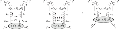
Figure 3: Illustration of $(z,k_{t})$-factorization for the doubly-unintegrated gluon distribution, $f_{g}(x,z,k_{t}^{2},\mu^{2})$, shown in the final diagram. In the first two diagrams the penultimate parton in the DGLAP evolution chain, with 4-momentum $k_{n-1}=(x/z)\,p$, splits into a gluon with 4-momentum $k_{n}\equiv k=x\,p-\beta\,q^{\prime}+k_{\perp}$.

It is not immediately obvious how the partonic cross sections $\hat{\sigma}^{\gamma^{*}a^{*}}$ in (16) should be calculated. Recall that they can be written

$$\hat{\sigma}=\int\!\mathrm{d}\Phi\,\lvert\mathcal{M}\rvert^{2}\,/\,F,$$ (17)

where $\mathrm{d}\Phi$ is the phase space element, $\lvert\mathcal{M}\rvert^{2}$ is the squared matrix element, and $F$ is the flux factor. The phase space element $\mathrm{d}\Phi$ can be calculated with the full kinematics, that is, with $k=x\,p-\beta\,q^{\prime}+k_{\perp}$. The flux factor $F$ is taken to be the same as in collinear factorization (and in $k_{t}$-factorization), that is, $F=4x\,p\cdot q$. The last evolution steps in Fig. 3 only factorize from the rest of the diagram, to give the LO DGLAP splitting kernels, in the leading logarithmic approximation (LLA), that is, in either the collinear ($k_{t}\to 0$) or high-energy ($z\to 0$) limits. Therefore, $\lvert\mathcal{M}\rvert^{2}$ should be evaluated with either $k=x\,p$ or $k=x\,p+k_{\perp}$, in order to provide the factorization between the DUPDF and the subprocess labeled $\hat{\sigma}$ in Fig. 3. For the specific case of inclusive jet production in DIS and working in an axial gluon gauge, it was observed in Watt:2003mx that the main effect of the “beyond LLA” terms (proportional to $\beta$ (12)) was to suppress soft gluon emission, and that these terms made a negligible difference to the cross section when the angular-ordering constraints were applied.

The prescription adopted in Watt:2003mx was to evaluate $\lvert\mathcal{M}\rvert^{2}$ in the collinear approximation ($k=x\,p$), so that a $(z,k_{t})$-factorization calculation approximately reproduces the collinear factorization calculation starting one rung down as in the first two diagrams of Fig. 3, that is, where the subprocess is evaluated at one order higher in $\alpha_{S}$. This was demonstrated for inclusive jet production in DIS, where the LO subprocess is simply $\gamma^{*}q^{*}\to q$. Similarly, a “NLO” calculation, where the subprocesses are $\gamma^{*}g^{*}\to q\bar{q}$ and $\gamma^{*}q^{*}\to qg$, was found to give results close to the conventional NLO QCD calculation, where the subprocesses are $\mathcal{O}(\alpha_{S}^{2})$; see Fig. 4.

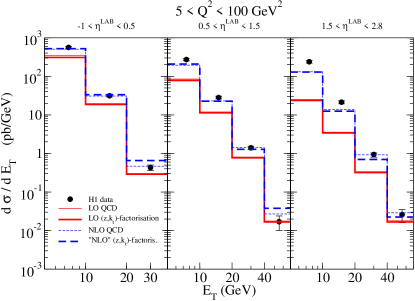
Figure 4: Comparison with H1 inclusive jet production data Adloff:2002ew in three pseudorapidity ($\eta^{\textsc{lab}}$) bins. The predictions of the $(z,k_{t})$-factorization approach based on DUPDFs Watt:2003mx (which is much simpler to implement) are in good agreement with the conventional QCD approach. In some bins the predictions of the latter approach are hidden beneath the bold lines of the $(z,k_{t})$-factorization approach, at the respective order.

In Watt:2003vf , the $(z,k_{t})$-factorization formalism was extended to hadron–hadron collisions and applied to predict the $p_{T}$ distributions of vector bosons ($V=W,Z$) and Standard Model Higgs bosons ($H$). For $p_{T}\ll M_{V,H}$, fixed-order collinear factorization calculations diverge, with $\ln(M_{V,H}/p_{T})$ terms appearing in the perturbation series due to soft and collinear gluon emission. Traditional calculations combine fixed-order perturbation theory at high $p_{T}$ with either analytic resummation or numerical DGLAP-based parton shower formalisms at low $p_{T}$, with some matching criterion to decide when to switch between the two. It has been shown in Gawron:2003np ; Kwiecinski:2003fu that UPDFs obtained from an approximate solution of the CCFM evolution equation embody the conventional soft gluon resummation formulae. In the framework of $(z,k_{t})$-factorization, the lowest order subprocesses are simply $q_{1}^{*}\,q_{2}^{*}\to V$ and $g_{1}^{*}\,g_{2}^{*}\to H$. A good description was obtained in Watt:2003vf of the $p_{T}$ distributions of $W$ and $Z$ bosons produced at the Tevatron Run 1 over the whole $p_{T}$ range; see Fig. 5.

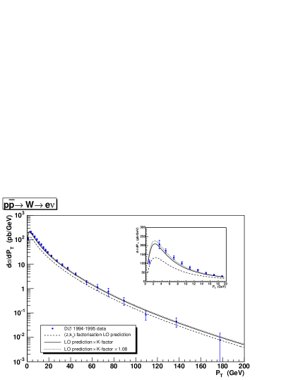
Figure 5: $p_{T}$ distribution of W bosons produced at the Tevatron calculated using $(z,k_{t})$-factorization Watt:2003vf , compared to DØ data Abbott:2000xv .

The predicted Higgs $p_{T}$ distribution at the LHC was found to reproduce, to a fair degree, the predictions of more elaborate theoretical studies Balazs:2004rd , in particular the NNLL+NLO resummation approach of Grazzini et al. Bozzi:2003jy ; see Fig. 6.

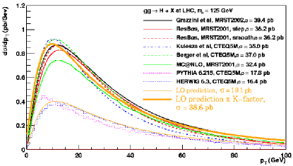
Figure 6: $p_{T}$ distribution of SM Higgs bosons produced at the LHC with mass 125 GeV calculated using $(z,k_{t})$-factorization Watt:2003vf , compared to various resummed and parton shower predictions which are all matched to fixed-order calculations at large $p_{T}$ (apart from herwig) Balazs:2004rd .

Alternative predictions for Higgs production at the LHC using the $k_{t}$-factorization approach have been made in Gawron:2003np ; Jung:2003wu ; Lipatov:2005at ; Luszczak:2005xs .

Note that matrix-element corrections are necessary in DGLAP-based parton shower simulations at large $p_{T}$. Without such corrections, the herwig parton shower prediction falls off dramatically at large $p_{T}\gtrsim M_{H}$ Corcella:2004fr ; see Fig. 6. The same effect is observed in herwig predictions for the $p_{T}$ distributions of $W$ and $Z$ bosons Corcella:1999gs , whereas in Fig. 5 the Tevatron data at large $p_{T}\gtrsim M_{W}$ are well-described without explicit matrix-element corrections. Also, the $(z,k_{t})$-factorization prediction for Higgs production is found to be close to the NLO fixed-order result at large $p_{T}$, see Fig. 6, suggesting that a large part of the subleading terms are included by accounting for the precise kinematics in the $g_{1}^{*}\,g_{2}^{*}\to H$ subprocess.

The integrated PDFs used as input in Watt:2003mx ; Watt:2003vf were determined from a global fit to data using the conventional collinear approximation Martin:2002dr . A more precise treatment would determine the integrated PDFs, used as input to the last evolution step, from a new global fit to data using the $(z,k_{t})$-factorization formalism.

2.4 NLO BFKL

Main author J. Andersen and A. Sabio-Vera

Since the completion of the calculation of the next–to–leading (NLL) corrections to the BFKL equation Fadin:1998py ; Ciafaloni:1998gs for the forward kernel there has been a large activity focused on the study of the fundamental properties of the NLL gluon Green’s function in the Regge limit of QCD at high energies Ross:1998xw ; Salam:1998tj ; Ciafaloni:2003kd ; Ciafaloni:2003rd ; Ciafaloni:2003ek ; Ciafaloni:2002xk ; Ciafaloni:2002xf ; Ciafaloni:2000cb ; Ciafaloni:1999au ; Ciafaloni:1999yw ; Ciafaloni:1998iv ; Forshaw:1999xm ; Forshaw:2000hv ; Kovchegov:1998ae ; Schmidt:1999mz ; Altarelli:2003hk ; Altarelli:2001ji ; Altarelli:2000mh ; Altarelli:1999vw . Recently, a powerful approach has been developed which allows for the complete and exact analysis of the solution at NLL. In Ref. Andersen:2003an it was demonstrated how it is possible to use $D=4+2\epsilon$ dimensional regularization together with an effective gluon mass ($\lambda$) to explicitly show the cancellation of simple and double poles in $\epsilon$. This procedure carries a logarithmic dependence in $\lambda$ which numerically cancels out when the full NLL BFKL evolution is taken into account for a given center–of–mass energy, this being a natural consequence of the infrared finiteness of the full kernel. The basis of this approach is the iterated form of the solution for the NLL BFKL equation, i.e.

$$\begin{split}&f({\bf k}_{a},{\bf k}_{b},{\rm Y})=e^{\omega_{0}^{\lambda}\left({\bf k}_{a}\right){\rm Y}}\left\{\frac{}{}\delta^{(2)}({\bf k}_{a}-{\bf k}_{b})\right.\\ &\hskip 14.22636pt+\sum_{n=1}^{\infty}\prod_{i=1}^{n}\int d^{2}{\bf k}_{i}\left[\frac{\theta\left({\bf k}_{i}^{2}-\lambda^{2}\right)}{\pi{\bf k}_{i}^{2}}\xi\left({\bf k}_{i}\right)+\right.\\ &\hskip 99.58464pt\left.\widetilde{\mathcal{K}}_{r}\left({\bf k}_{a}+\sum_{l=0}^{i-1}{\bf k}_{l},{\bf k}_{a}+\sum_{l=1}^{i}{\bf k}_{l}\right)\frac{}{}\right]\\ &\hskip 28.45274pt\left.\times\int_{0}^{y_{i-1}}dy_{i}~{}e^{\left(\omega_{0}^{\lambda}\left({\bf k}_{a}+\sum_{l=1}^{i}{\bf k}_{l}\right)-\omega_{0}^{\lambda}\left({\bf k}_{a}+\sum_{l=1}^{i-1}{\bf k}_{l}\right)\right)y_{i}}\right.\\ &\hskip 85.35826pt\left.\delta^{(2)}\left(\sum_{l=1}^{n}{\bf k}_{l}+{\bf k}_{a}-{\bf k}_{b}\right)\right\},\end{split}$$ (18)

where the strong ordering in longitudinal components of the parton emission is encoded in the nested integrals in rapidity with an upper limit set by the logarithm of the total energy in the process, $y_{0}={\rm Y}$. The Reggeized form of the gluon propagators in the $t$–channel, $\omega_{0}^{\lambda}\left({\bf q}\right)$, in this approach reads

$$\begin{split}\omega_{0}^{\lambda}\left({\bf q}\right)=-\bar{\alpha}_{s}&\ln{\frac{{\bf q}^{2}}{\lambda^{2}}}+\frac{\bar{\alpha}_{s}^{2}}{4}\left[\frac{\beta_{0}}{2N_{c}}\ln{\frac{{\bf q}^{2}}{\lambda^{2}}}\ln{\frac{{\bf q}^{2}\lambda^{2}}{\mu^{4}}}\right.\\ &+\left.\left(\frac{\pi^{2}}{3}-\frac{4}{3}-\frac{5}{3}\frac{\beta_{0}}{N_{c}}\right)\ln{\frac{{\bf q}^{2}}{\lambda^{2}}}+6\zeta(3)\right]\end{split}$$ (19)

with

$$\xi\left({\rm X}\right) \equiv \bar{\alpha}_{s}+\frac{{\bar{\alpha}_{s}}^{2}}{4}\left(\frac{4}{3}-\frac{\pi^{2}}{3}+\frac{5}{3}\frac{\beta_{0}}{N_{c}}-\frac{\beta_{0}}{N_{c}}\ln{\frac{{\rm X}}{\mu^{2}}}\right)$$ (20)

being the corresponding part in the real emission kernel. To complete the real part of the NLL kernel there are other more complicated terms in $\tilde{\cal K}_{r}$ which do not generate $\epsilon$ singularities when integrated over the full phase space of the emissions, for details see Ref. Andersen:2003an .

The numerical implementation and analysis of the form of solution as in Eq. (18) was carried out in Ref. Andersen:2003wy . At the light of this study the known feature of a lower intercept at NLL with respect to leading–order (LL) was confirmed. As in this approach it is not needed to expand on any eigenfunctions there are no instabilities in the energy growth. This is highlighted at the left hand side of Fig. 7 where the bands correspond to uncertainties in the choice of renormalization scale.

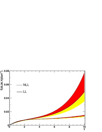
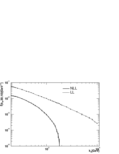
Figure 7: Analysis of the gluon Green’s function as obtained from the NLL BFKL equation.

However, the space where the convergence of the perturbative expansion is poor is not in energy but in transverse momenta. In particular, when the two transverse scales entering the forward gluon Green’s function are of comparable magnitude then the NLL corrections are smaller when compared to LL, this can be seen in the bottom plot of Fig 7. However when the ratio between these scales largely departs from unity then the $|{\rm NLL-LL}|$ difference becomes large, driving, as it is well–known, the gluon Green’s function into an oscillatory behavior with negative values.

The main advantage of the method here described is that the Green’s function is generated integrating the phase space using a Monte Carlo sampling of the different parton configurations. This feature allows for a full control of the average multiplicities and angular dependences. The former can be extracted from the Poisson–like distribution in the number of rungs, or iterations of the kernel, needed to reach a convergent solution. This is obtained numerically in the upper part of Fig. 8, where we see e.g. that for $Y=5$ it is should be enough to include $\sim 15$ rungs/iterations. At the lower part of the same figure the angular correlations in the azimuthal angle of dijets with similar and large transverse energy, and low hadronic activity in between, is studied in a toy cross–section with simplified impact factors. The increase of the angular correlation when the NLL terms are included in such observable is a characteristic feature of these corrections. This study is possible within this approach in an immediate manner because the NLL kernel is treated in full, without angular averaging, so there is no need to use a Fourier expansion in angular variables via the introduction of conformal spins.

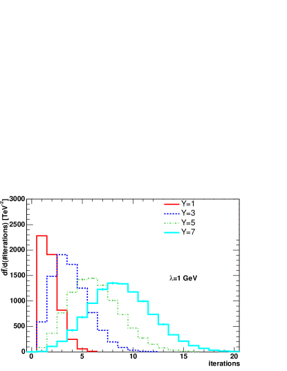
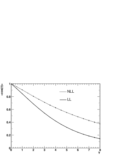
Figure 8: Distribution in the number of iterations and angular dependence of the NLL gluon Green’s function.

An interesting theoretical development in the context of NLL BFKL was the calculation of the forward NLL kernel in the conformally invariant $N=4$ super Yang–Mills theory Kotikov:2000pm ; Kotikov:2002ab . In such field theory the coupling remains a constant even at NLL, opening the possibility of finding the solution of the BFKL equation in a straightforward way because the LL eigenfunctions are also so at NLL. In particular, the kernel was calculated for all conformal spins in Ref. Kotikov:2000pm ; Kotikov:2002ab allowing for the direct test of the angular structure of the solution as obtained from the method here described. This comparison between both approaches was performed in Ref. Andersen:2004uj . In this case the gluon Regge trajectory reads (with $a$ denoting the coupling constant)

$$\omega_{0}^{\lambda}\left({\bf{q}}\right)=-a\ln{\frac{\bf{q}^{2}}{\lambda^{2}}}+\frac{a^{2}}{4}\left[\left(\frac{\pi^{2}}{3}-\frac{1}{3}\right)\ln{\frac{\bf{q}^{2}}{\lambda^{2}}}+6\,\zeta(3)\right]$$ (21)

and $\xi=a+a^{2}\left(\frac{1}{12}-\frac{\pi^{2}}{12}\right)$ is a constant without logarithmic dependence. For a precise determination of the contribution to the gluon Green’s function stemming from the different Fourier components in the azimuthal angle, i.e.

$$f\left(\bf{k}_{a},\bf{k}_{b},{\rm Y}\right)=\sum_{n=-\infty}^{\infty}f_{n}\left(|\bf{k}_{a}|,|\bf{k}_{b}|,{\rm Y}\right)e^{in\theta},$$ (22)

it is enough to extract the coefficients of the expansion, either using the kernel calculated in Kotikov:2000pm ; Kotikov:2002ab

$$f_{n}\left(|\bf{k}_{a}|,|\bf{k}_{b}|,{\rm Y}\right)=\frac{1}{\pi|\bf{k}_{a}||\bf{k}_{b}|}\int\frac{d\gamma}{2\pi i}\left(\frac{\bf{k}_{a}^{2}}{\bf{k}_{b}^{2}}\right)^{\gamma-\frac{1}{2}}e^{\omega_{n}(a,\gamma){\rm Y}},$$ (23)

or making use of the iterative solution explained in this section Andersen:2004uj :

$$f_{n}\left(|\bf{k}_{a}|,|\bf{k}_{b}|,{\rm Y}\right)=\int_{0}^{2\pi}\frac{d\theta}{2\pi}\,f\left(\bf{k}_{a},\bf{k}_{b},{\rm Y}\right)\cos{\left(n\theta\right)}.$$ (24)

The results from these two independent alternatives are shown to coincide in Fig. 9. In the upper part the $n=0$ Fourier component clearly dominates at large energies, decreasing the angular correlations as the energy increases. In the lower part it is shown how the convergence in the angular variable on the transverse plane is achieved after only a few terms in the Fourier expansion for different values of the available energy in the scattering process.

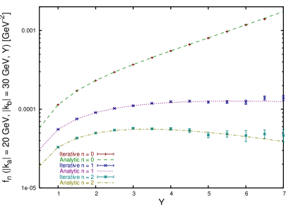
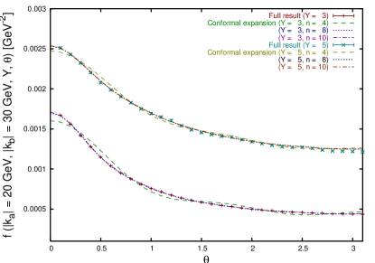
Figure 9: Projections on conformal spins of the N=4 SUSY NLL BFKL Green’s function.

In this section a new analysis of the gluon Green’s function as obtained from the NLL BFKL kernel has been presented. The method of solution is based on the Monte Carlo integration of the phase space of different partonic configurations in the multi–Regge and quasi–multi–Regge kinematics. This method has many advantages with respect to previous analysis of the same problem. It allows for a reliable study of angular dependences in a straightforward manner, the multiplicities in the evolution are under control, and it provides an exact solution even with running coupling terms which break the scale invariance in the kernel. Many other studies are on their way using this procedure, as for example, deep inelastic scattering, the non–forward case and the matching of this solution to different impact factors for the final calculation of cross–sections at NLL where the BFKL approach will be relevant at present and planned colliders.

2.5 Resummation at small $x$

Main author A. Stasto

The large magnitude of the NLLx correction in the high energy limit, as well as the instabilities associated with it, motivate the study of the resummation procedure in the limit of small $x$. In particular it has been observed that, by taking into account collinear limits correctly in the NLLx equation, as it is required by the DGLAP dynamics, stabilizes the high energy expansion. To understand this in more detail let us recall the structure of the LLx BFKL equation in the Mellin space where the Mellin variable $\gamma$ is conjugated to the logarithm of the transverse momentum $\ln k_{T}^{2}/\Lambda^{2}$

$$\chi^{(0)}(\gamma)\;=\;2\psi(1)-\psi(\gamma)-\psi(1-\gamma)\;\sim\;\frac{1}{\gamma}+\frac{1}{1-\gamma}$$ (25)

where in the pole expansion of the kernel eigenvalue we have retained only leading collinear and anticollinear poles. These correspond exactly to the DGLAP strong ordering of transverse momenta along the gluon ladder. In the NLLx case the eigenvalue function takes on a complicated functional form which in the collinear limit is

$$\chi^{(1)}(\gamma)\simeq\frac{A_{1}(0)}{\gamma^{2}}+\frac{A_{1}(0)}{(1-\gamma)^{2}}-\frac{1}{2\gamma^{3}}-\frac{1}{2(1-\gamma)^{3})}+{\cal O}(\frac{1}{\gamma},\frac{1}{1-\gamma})$$ (26)

with $A_{1}(0)=-11/12$. Note the negative sign of the NLLx contribution. It turns out that the collinear approximation above reproduces the exact result within $\sim 7\%$ of accuracy. The terms proportional to $A_{1}(0)$ are related to the non-singular in $x$ part of the LO DGLAP splitting function, whereas the cubic poles come from the energy scale choice. The highly singular form of the NLLx correction as it is seen from eq.(26) is the source of the large correction and potentially unstable behavior. The resummation procedure presented in Ciafaloni:1999yw is based on four key ingredients:

• Taking into account the full splitting function at LO in the DGLAP approximation.

• Incorporating the energy scale change in the form of the kinematical constraint.

• Running of the coupling constant $\alpha_{s}$

• Subtraction of the double and single poles in order to avoid double counting.

In Ciafaloni:2003rd a procedure based on the numerical solution of the BFKL equation in momentum space was presented. It takes into account all of the above-mentioned ingredients and yields stable result for the intercept and the gluon Green’s function. Furthermore, the procedure for extraction the resummed splitting function was also presented, which is more relevant for application to the deep inelastic scattering processes such as measured at HERA. In Fig.2.5 we show the resummed splitting function obtained in the resummed scheme Ciafaloni:2003rd , together with the renormalization scale variation and the singular in $x$ part of the NNLO DGLAP splitting function.

The characteristic feature of the resummed splitting function $P_{gg}$ is the strong preasymptotic behavior at intermediate values of $x\simeq 10^{-3}-10^{-4}$ which manifests itself in the dip of the splitting function, only later followed by the increase at very small $x$. Also interesting is the fact that the small $x$ part of the NNLO DGLAP splitting function matches nearly exactly with the initial decrease of the resummed splitting function. The existence of the dip rather than an increase at values of $x\sim 10^{-4}$ can have an interesting impact on the phenomenology.

2.6 The NLO ${\gamma^{*}}$ impact factor

Main author A. Kyrieleis

One of the most attractive observables to test the BFKL approach is the total cross section for ${\gamma^{*}}{\gamma^{*}}$ scattering. To calculate this observable in the framework of NLO BFKL the ${\gamma^{*}}$ impact factor ($\Phi$) at NLO is needed in addition to the universal BFKL Green function (G), see Fig.10.

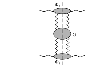
Figure 10: $\sigma_{tot}^{\gamma^{*}\gamma^{*}}$ in the framework of BFKL

If the NLO BFKL equation is solved in the momentum space the numerical value of the ${\gamma^{*}}$ impact factor has to be known as a function of the Reggeon momentum and of the energy scale.

Besides this, the NLO ${\gamma^{*}}$ impact factor allows to approach the resummation of the next-to-leading logs(1/x) in the quark anomalous dimensions. It also provides the full information necessary to investigate the color dipole picture at NLO which, at LO, is one of the important ingredients to the QCD evolution based upon the Balitsky-Kovchegov equation (see section 5 below). At the first small-x workshop Andersson:2002cf first steps in the calculation of this impact factor have been presented.

The virtual and the real corrections of the ${\gamma^{*}}$ impact factor are calculated from the photon-Reggeon vertices for $q\bar{q}$ and $q\bar{q}g$ production, respectively. Both vertices are known Bartels:2000gt ; Fadin:2001ap ; Bartels:2001mv ; Bartels:2002uz . What remains to complete the calculation of the NLO photon impact factor after the infrared divergences of the virtual and of the real parts have been combined Bartels:2002uz are the integrations over the $q\bar{q}$ and $q\bar{q}g$ phase space, respectively.

Recently, the phase space integration in the real corrections have been performed for the case of longitudinal photon polarization, Bartels:2004bi . The integration over the transverse momenta have been carried out analytically. To this end the Feynman diagrams were treated separately giving rise to additional divergences that have been regularized. As the result, a convergent Feynman parameter integral has been obtained for each Feynman diagram (or small groups of them). These results can serve as a starting point for further analytical investigations, in particular because the Mellin transform of the real corrections w.r.t the Reggeon momentum can be easily obtained.

The remaining integrations in the real corrections (longitudinal ${\gamma^{*}}$ polarization) have been carried out numerically Bartels:2004bi . The result is a function $\Phi^{real}$ of two dimensionless (scaled by the photon virtuality) variables: the Reggeon momentum ${\bf r}^{2}$ and the energy scale $s_{0}$. A physical scattering amplitude (e.g. for the ${\gamma^{*}}{\gamma^{*}}$ scattering process) involving the BFKL Green’s function and the impact factors has to be invariant under changes of $s_{0}$. The $s_{0}$ dependence of the ${\gamma^{*}}$ impact factor therefore represents an important issue. $s_{0}$ enters the NLO ${\gamma^{*}}$ impact factor as a cutoff to exclude that region of the $q{\bar{q}}g$ phase space where the gluon is separated in rapidity from the $q{\bar{q}}$ pair (LLA). The virtual corrections are therefore independent of $s_{0}$ and the integration of the real corrections alone already allows to study the $s_{0}$ dependence of the NLO ${\gamma^{*}}$ impact factor. Let us define, as part of the full NLO impact factor:

$$\Phi^{\prime}=g^{2}\Phi^{(0)}+g^{4}\Phi^{\mathrm{r}eal}$$

where $g^{2}\Phi^{(0)}$ denotes the LO ${\gamma^{*}}$ impact factor and $g^{2}=4\pi\alpha_{s}$.

Figure 11: $\Phi^{\prime}$ at different different values of $s_{0}$

Choosing $Q^{2}=15$ GeV² for the photon virtuality leads $\alpha_{s}(Q^{2})=0.18$ or $g=1.5$. Fig.11 compares $\Phi^{\prime}$ to the LO impact factor as function of ${\bf r}^{2}$ at different values of $s_{0}$. The real corrections are negative and rather large. More important, $\Phi^{\prime}$ becomes, in absolute terms, more significant for smaller values of $s_{0}$. This implies that the ${\gamma^{*}}$ impact factor tends to become smaller with decreasing $s_{0}$. Since a decrease of $s_{0}$ in the energy dependence $(\frac{s}{s_{0}})^{\omega}$ will enhance the scattering amplitude, the combined $s_{0}$ dependence of the impact factors and the BFKL Green’s function has to compensate this growth. The result for the $s_{0}$ behavior of the ${\gamma^{*}}$ impact factor is therefore, at least, consistent with the general expectation. To check the $s_{0}$ (in)dependence of the full scattering amplitude and to compute $\sigma^{{\gamma^{*}}{\gamma^{*}}}$, at least for longitudinal ${\gamma^{*}}$ polarization, the phase space integration in the virtual corrections is the only piece missing.

3 Applications of $k_{\perp}$-factorization

In collinear factorisation the transverse momenta of the incoming partons are neglected whereas they are included in $k_{\perp}$-factorization if the same order in $\alpha_{s}$  of the calculation is considered. Thus in collinear factorsiation these transverse momentum effects come in as a next-to-leading order level.

In the following sections we discuss some applications of $k_{\perp}$-factorization to describe heavy quark production in $p\bar{p}$ collisions.

3.1 Heavy quark production at the Tevatron

Main author N. Zotov

Heavy quark production in hard collisions of hadrons has been considered as a clear test of perturbative QCD. Such processes provide also some of the most important backgrounds to new physics phenomena at high energies.

Bottom production at the Tevatron in the $k_{\perp}$-factorization approach was considered earlier in Levin:1991ry ; Ryskin:1995sj ; Ryskin:2000bz ; Ryskin:1999yq ; Hagler:2000dd ; Jung:2001rp ; Baranov:2000gv ; Lipatov:2001ny . Here we use the $k_{\perp}$-factorization approach for a more detailed analysis of the experimental data Abbott:1999se ; Abe:1996zt ; Acosta:2002qk ; Acosta:2001rz ; Abbott:1999wu . The analysis also covers the azimuthal correlations between $b$ and $\bar{b}$ quarks and their decay muons. Some of these results have been presented earlier in Refs. Lipatov:2001ny ; Baranov:1999ja ; Baranov:2000uv ; Zotov:2003gc ; Lipatov:2002tc ; Kotikov:2001ct ; Kotikov:2002nh (see also Andersson:2002cf ; Andersen:2003xj ).

3.2 Theoretical framework

In the $k_{\perp}$-factorization approach, the differential cross section for inclusive heavy quark production may be written as (see  Baranov:2004eu )

$$d\sigma(p\bar{p}\to Q\bar{Q}\,X)=$$

$${1\over 16\pi(x_{1}\,x_{2}\,s)^{2}}\,\mathcal{A}(x_{1},{\mathbf{q}}_{1T}^{2},\mu^{2})\,\mathcal{A}(x_{2},{\mathbf{q}}_{2T}^{2},\mu^{2})$$

$$\times \sum{|M|^{2}_{{\rm SHA}}(g^{*}g^{*}\to Q\bar{Q})}$$

$$\times dy_{1}\,dy_{2}\,d{\mathbf{p}}_{2T}^{2}\,d{\mathbf{q}}_{1T}^{2}\,d{\mathbf{q}}_{2T}^{2}{d\phi_{1}\over 2\pi}\,{d\phi_{2}\over 2\pi}\,{d\phi_{Q}\over 2\pi},$$ (27)

where $\mathcal{A}(x_{1},{\mathbf{q}}_{1T}^{2},\mu^{2})$ and $\mathcal{A}(x_{2},{\mathbf{q}}_{2T}^{2},\mu^{2})$ are unintegrated gluon distributions in the proton, ${\mathbf{q}}_{1T}$, ${\mathbf{q}}_{2T}$, ${\mathbf{p}}_{2T}$ and $\phi_{1}$, $\phi_{2}$, $\phi_{Q}$ are transverse momenta and azimuthal angles of the initial BFKL gluons and final heavy quark respectively, $y_{1}$ and $y_{2}$ are the rapidities of heavy quarks in the $p\bar{p}$ center of mass frame. $\sum{|M|^{2}_{{\rm SHA}}(g^{*}g^{*}\to Q\bar{Q})}$ is the off mass shell matrix element, where the symbol $\sum$ in (27) indicates an averaging over initial and a summation over the final polarization states. The expression for $\sum{|M|^{2}_{{\rm SHA}}(g^{*}g^{*}\to Q\bar{Q})}$ coincides with the one presented in Catani:1991eg .

In the numerical analysis, we have used the KMS parameterization Kwiecinski:1997ee for the $k_{\perp}$-dependent gluon density. It was obtained from a unified BFKL and DGLAP description of $F_{2}$ data and includes the so called consistency constraint Kwiecinski:1996td . The consistency constraint introduces a large correction to the LO BFKL equation; about 70% of the full NLO corrections to the BFKL exponent $\lambda$ are effectively included in this constraint, as is shown in Kwiecinski:1996td ; Kwiecinski:1999hv .

3.3 Numerical results

In this section we present the numerical results of our calculations and compare them with $B$-meson production at D0 Abbott:1999se ; Abbott:1999wu , CDF Abe:1996zt ; Acosta:2002qk ; Acosta:2001rz and UA1 Albajar:1993be .

Besides the choice of the unintegrated gluon distribution, the results depend on the bottom quark mass, the factorization scale $\mu^{2}$ and the $b$ quark fragmentation function. As an example, Ref. Cacciari:2002pa used a special choice of the $b$-quark fragmentation function, as a way to increase the $B$ meson cross section in the observable range of transverse momenta. In the present paper we convert $b$ quarks into $B$ mesons using the standard Peterson fragmentation function  Peterson:1982ak with $\epsilon=0.006$. Regarding the other parameters, we use $m_{b}=4.75\,{\rm GeV}$ and $\mu^{2}={\mathbf{q}}_{T}^{2}$ as in Levin:1991ry ; Hagler:2000dd .

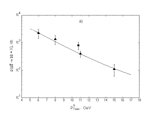
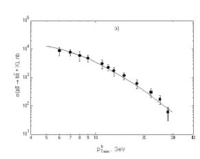
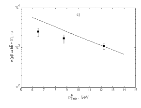
Figure 12: The $b$ quark transverse momentum distribution (integrated from $p_{T\min}^{b}$) at Tevatron conditions presented in the form of integrated cross sections. The curves correspond to the $k_{\perp}$-factorization results with the KMS unintegrated gluon distribution. Experimental data are from UA1 Albajar:1993be (Fig. a)), D0 Abbott:1999se (Fig. b)), and CDF Abe:1996zt ; Acosta:2002qk (Fig. c)).

The results of the calculations are shown in Figs. 12-16. Fig. 12 displays the $b$ quark transverse momentum distribution at Tevatron conditions presented in the form of integrated cross sections. The following cuts were applied: (a) $|y_{1}|<1.5$, $|y_{2}|<1.5$, $\sqrt{s}=630\,{\rm GeV}$; (b) $|y_{1}|<1$, $\sqrt{s}=1800\,{\rm GeV}$; and (c) $|y_{1}|<1$, $|y_{2}|<1$, $\sqrt{s}=1800\,{\rm GeV}$. One can see reasonable agreement with the experimental data.

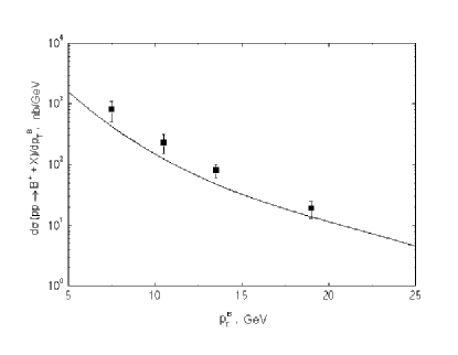
Figure 13: Theoretical predictions for the $B$ meson $p_{T}$ spectrum compared to the CDF Acosta:2001rz data. Curve is the same as in Fig. 12.

Fig. 13 shows the prediction for the $B$ meson $p_{T}$ spectrum at $\sqrt{s}=1800\,{\rm GeV}$ compared to the CDF data Abe:1996zt within the experimental cuts $|y|<1$, where also a fair agreement is found between results obtained in the $k_{\perp}$-factorization approach and experimental data.

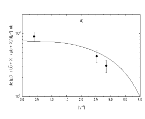
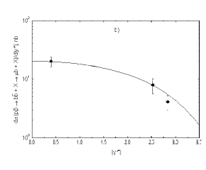
Figure 14: The cross section for muons from $B$ meson decay as a function of rapidity compared to the D0 data Abbott:1999wu . The curves are the same as in Fig. 12.

The D0 data include also muons originating from the semileptonic decays of $B$-mesons. To produce muons from $B$ mesons in theoretical calculations, we simulate their semileptonic decay according to the standard electroweak theory. In Fig. 14 we show the rapidity distribution $d\sigma/d|y^{\mu}|$ for decay muons with $p_{T}^{\mu}>5\,{\rm GeV}$.

Fig. 15 shows the leading muon $p_{T}$ spectrum for $b\bar{b}$ production events compared to the D0 data. The cuts applied to both muons are given by $4<p_{T}^{\mu}<25\,{\rm GeV}$, $|\eta^{\mu}|<0.8$ and $6<m^{\mu\mu}<35\,{\rm GeV}$. The leading muon in the event is defined as the muon with largest $p_{T}^{\mu}$-value. In all the above cases a rather good description of the experimental measurements is achieved.

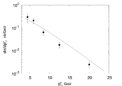
Figure 15: Predictions for the leading muon $p_{T}$ spectrum in the $b\bar{b}$ production events compared to the D0 data Abbott:1999se . The curve is the same as in Fig. 12.

It has been pointed out that investigations of $b\bar{b}$ correlations, such as the azimuthal opening angle between $b$ and $\bar{b}$ quarks (or between their decay muons), allow additional details of the $b$ quark production to be tested, since these quantities are sensitive to the relative contributions of the different production mechanisms Levin:1991ry ; Ryskin:1995sj ; Ryskin:2000bz ; Ryskin:1999yq ; Hagler:2000dd ; Baranov:2000gv . In the collinear approach at LO the gluon-gluon fusion mechanism gives simply a delta function, $\delta(\Delta\phi^{b\bar{b}}-\pi)$, for the distribution in the azimuthal angle difference $\Delta\phi^{b\bar{b}}$. In the $k_{\perp}$-factorization approach the non-vanishing initial gluon transverse momenta, $q_{1T}$ and $q_{2T}$, implies that this back-to-back quark production kinematics is modified. In the collinear approximation this effect can only be achieved if NLO contributions are included.

The differential $b\bar{b}$ cross section $d\sigma/d\Delta\phi^{\mu\mu}$ is shown in Fig. 16 (from Baranov:2004eu ). The following cuts were applied to both muons: $4<p_{T}^{\mu}<25\,{\rm GeV}$, $|\eta^{\mu}|<0.8$ and $6<m^{\mu\mu}<35\,{\rm GeV}$. We note a significant deviation from the pure back-to-back production, corresponding to $\Delta\phi^{\mu\mu}\approx\pi$. There is good agreement between the KMS prediction and the experimental data, which shows that for these correlations the $k_{\perp}$-factorization scheme with LO matrix elements very well reproduces the NLO effects due to the gluon evolution.

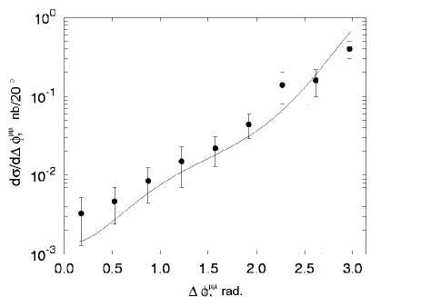
Figure 16: Azimuthal muon-muon correlations at Tevatron conditions. The curve is the same as in Fig. 12. Experimental data are from the D0 collaboration Abbott:1999se .

3.4 Quarkonium production

Main author S. Baranov

The $k_{\perp}$-factorization approach has rather successfully described the production of open charm and beauty, as discussed in the previous section, but also hadroproduction of heavy quarkonium states, $J/\psi$, $\chi_{c}$ and $\Upsilon$ mesons, at the Tevatron are well describedHagler:2000dd ; Hagler:2000eu ; Yuan:2000cp ; Yuan:2000qe . In many cases, however, the data can also be described within the usual collinear parton model, if the relevant next-to-leading order QCD corrections are taken into account, or if the so called color-octet mechanism is included.

In this context, the theoretical predictions on $J/\psi$ spin alignment made in Ref. Baranov:1998af are of particular interest, as the collinear and $k_{\perp}$-factorization approaches show qualitatively different behavior. Note that the $k_{\perp}$-factorization approach provides the only known (up to date) explanation of the $J/\psi$  polarization phenomena observed at the Tevatron Baranov:2002cf and at HERA Lipatov:2002tc .

It would be interesting and important to find other examples, where the difference between the collinear and noncollinear approaches would be manifested in a clear and unambiguous way. In this section we suggest such a process. We analyze the production of $P$-wave quarkonium states (namely the $\chi_{c}$ and $\chi_{b}$ mesons) in high energy hadronic collisions and demonstrate the dramatic difference between the different theoretical calculations.

Naively one could expect a difference from the fact that the production of $\chi_{1}$ states in the $2\to 1$ gluon-gluon fusion process is forbidden, if the initial gluons are on shell, but is allowed if the gluons are off shell. However, the real situation is complicated by the necessity to take into account also the $2\to 2$ processes. The results of our analysis are presented in the next subsection.

We begin our discussion with showing the predictions of the collinear parton model for the production of $P$-wave charmonia at Tevatron conditions. The color-singlet production scheme refers to the $2\to 2$ gluon-gluon fusion subprocess

$$g+g\to\chi+g.$$ (28)

(It would be inadequate to rely upon the $2\to 1$ subprocess $g+g\to\chi$ in this case, because the final state particle would then be produced with zero transverse momentum, and thus could not be detected experimentally.) The computational technique is explained in detail elsewhere Krasemann:1978jc ; Guberina:1980dc ; Kniehl:2003pc .

For the sake of definiteness, we only present the parameter setting used in our calculations. Throughout the paper we use the LO GRV set Gluck:1994uf for gluon densities in the proton, and the value for the $\chi_{c}$ wave function, $|{\cal R}^{\prime}_{\chi_{c}}(0)|^{2}=0.075$ GeV⁵, taken from the potential model of Ref. Eichten:1995ch . The renormalization scale in the strong coupling constant $\alpha_{s}(\mu_{R}^{2}/\Lambda^{2})$ is set to $\mu_{R}^{2}=m_{\chi}^{2}+p_{T,\chi}^{2}$ with $\Lambda$=200 MeV. The integration over the final state phase space is restricted to the pseudorapidity interval $-0.6<\eta(\chi_{c})<0.6$, in accord with the experimental cuts used by the CDF collaboration Abe:1992ww ; Abe:1993vw ; Abe:1995dv ; Abe:1997yz ; Affolder:2001ij ; Affolder:1999wm .

Since in the collinear formalism the predictions based on the color-singlet mechanism alone are known to be inconsistent with the data Abe:1992ww ; Abe:1993vw ; Abe:1995dv ; Abe:1997yz ; Affolder:2001ij ; Affolder:1999wm , the theory has to be amplified with the so called color-octet contribution, as it is commonly assumed in the literature Kniehl:2003pc . Unlike the predictions of the color-singlet model, the size of the color-octet matrix elements are not calculable within the theory. Therefore, the corresponding numerical results are always shown with arbitrary normalizing factors (just chosen to fit the experimental data when possible).

The numerical predictions of the collinear parton model are summarized in Fig. 17 (upper panel). At relatively low transverse momenta, the production of $\chi_{c}$ states is dominated by the color singlet mechanism. The differential cross section $d\sigma/dp_{T}$ diverges when $p_{T}\to 0$ for $\chi_{2}$ states (dashed histogram), while it remains finite for $\chi_{1}$ states (solid histogram). The production of $\chi_{1}$ states at zero $p_{T}$ is suppressed (in accord with the Landau-Yang theorem), because in the limit of very soft final state gluons the $2\to 2$ gluon-gluon process degenerates into the $2\to 1$ process. The shape of the $\chi_{0}$ spectrum is similar to that of $\chi_{2}$ (up to an overall normalizing factor), and this spectrum is not shown in the figure.

The production of $\chi_{c}$ mesons at high $p_{T}$ is dominated by the color-octet contribution, which mainly comes from the ‘gluon fragmentation’ diagrams. Here, the perturbative production of ${}^{3}\!S_{1}$ color octet states,

$$g+g\to\;^{3}\!S_{1}^{8}+g,$$ (29)

is followed by a nonperturbative emission of soft gluons, which results in the formation of physical color singlet $\chi_{c}$ mesons:

$${}^{3}\!S_{1}^{8}\to\;^{3}\!P_{J}^{1}+ng.$$ (30)

As the co-produced gluons in eq. (30) are assumed to be soft, the momentum distribution of $\chi_{c}$ mesons is taken identical to that of the color-octet ${}^{3}S_{1}$ state in eq. (29). The nonperturbative matrix elements responsible for the process eq. (30) are related to the fictitious color-octet wave functions, which are used in calculations based on eq. (29) in place of the ordinary color-singlet wave function: $<0|{\cal O}_{8}|0>=(9/2\pi)\;|{\cal R}_{8}(0)|^{2}$.

It should be noted that the fragmentation of an almost on-shell transversely polarized gluon into a $\chi_{1}$ state via the emission of a single additional gluon, $g\to\;^{3}\!S_{1}^{8}\to\chi_{1}+g$, is suppressed in accord with Landau-Yang theorem. In terms of the nonrelativistic approximation, it is equivalent to say that the formally leading color-electric dipole transitions are forbidden, and one must go to nonleading higher multipoles. As the degree of this suppression is not calculable within the color-octet model on its own, we rather arbitrarily set the suppression factor to 1/20, which corresponds to potential model expectations for the average value of $v^{2}$.

We now proceed with showing the results obtained in the $k_{\perp}$-factorization approach. In this case the production of charmonium $\chi_{c}$ states can be successfully described within the color-singlet model alone Baranov:2002cf , or with only a minor admixture of color-octet contributions Hagler:2000dd . The consideration is based on the $2\to 1$ partonic subprocess

$$g+g\to\chi,$$ (31)

which represents the true leading order in perturbation theory. The nonzero transverse momentum of the final state meson comes from the momenta of the initial gluons. The computational technique, which we are using here, is identical to the one described in detail in Ref. Baranov:2002cf .

Figure 17: Theoretical predictions for the production of $\chi_{c}$ mesons at Tevatron conditions. Upper: Predictions of the collinear parton model. Solid histogram, $\chi_{1}$ production via color-singlet mechanism; dashed histogram, $\chi_{2}$ production via color-singlet mechanism; the lower and the upper dotted histograms, $\chi_{1}$ and $\chi_{2}$ production via color-octet mechanism, respectively. Middle: Predictions of the $k_{\perp}$-factorization approach. Solid histograms, $\chi_{1}$ production; thin and thick dashed histograms, $\chi_{0}$ and $\chi_{2}$ production, respectively. The upper and the lower histograms of each type correspond to the gluon densities of Refs. Blumlein:1995eu and Gribov:1984tu . Only the color singlet mechanism is assumed in all cases. Lower: Predictions on the ratio of the differential cross sections $d\sigma(\chi_{1})/d\sigma(\chi_{2})$. Solid histograms, $k_{\perp}$-factorization approach with gluon densities of Refs. Blumlein:1995eu and Gribov:1984tu ; dashed histogram, collinear parton model, color singlet contribution only; dotted histograms, collinear parton model with both singlet and octet production mechanisms taken into account. The different curves from top to bottom correspond to the color-octet $\chi_{1}/\chi_{2}$ suppression factor set to 1, 0.3, 0.1 and 0.03, respectively.

Figure 18: Theoretical predictions on the production of $\chi_{b}$. The notations are the same as in Fig. 17.

In order to estimate the degree of theoretical uncertainty connected with the choice of unintegrated gluon density, we also use the prescription proposed in Gribov:1984tu . In this approach, the unintegrated gluon density is derived from the ordinary density $G(x,q^{2})$ by differentiating it with respect to $q^{2}$ and setting $q^{2}=k_{\perp}^{2}$. Among the different parameterizations available on the present-day theoretical market, this approach shows the largest difference with Blümlein’s density Blumlein:1995eu . Thus, these two gluon densities can represent a theoretical uncertainty band.

The numerical results are exhibited in Fig. 17 (middle panel). In contrast with the collinear parton model, the differential cross sections are no longer divergent, even at very low $p_{T}$ values. This property emerges from the fact that the relevant $2\to 1$ matrix elements are always finite. One can see that the production of the $\chi_{1}$ state (solid histogram) at low $p_{T}$ is strongly suppressed (in comparison with the $\chi_{0}$ and $\chi_{2}$ states, short and long dashed histograms) because the initial gluons are almost on-shell. The suppression goes away at higher $p_{T}$, as the off-shellness of the initial gluons becomes larger.

In Fig. 17 (lower panel) we compare the predictions of the collinear and $k_{\perp}$-factorization approaches by showing the ratio of the differential cross sections $d\sigma(\chi_{c1})/dp_{T}$ and $d\sigma(\chi_{c2})/dp_{T}$ plotted as a function of $p_{T}$. As long as the ratio of the nonperturbative color-octet matrix elements, ${\cal O}(^{3}S_{1}^{8}\to\chi_{1})/{\cal O}(^{3}S_{1}^{8}\to\chi_{2})$, is unknown, the predictions of the collinear parton model are very uncertain. The different dotted curves in Fig. 17 from top to bottom correspond to the color-octet $\chi_{1}/\chi_{2}$ suppression factor set to 1, 0.3, 0.1, and 0.03, respectively. The band between the two lowest histograms may be considered as the most realistic case. The predictions of the collinear and $k_{\perp}$-factorization approaches clearly differ from each other in their absolute values, and show just the opposite trend in the experimentally accessible region ($p_{T}>5$ GeV).

We conclude our discussion with showing the predictions for the bottomonium states. The calculations are performed with the parameter setting given above, and with the value of the $\chi_{b}$ wave function set equal to $|{\cal R}^{\prime}_{\chi_{b}}(0)|^{2}=1.4$ GeV⁵ Hagiwara:1986tu . The integration over the final state phase space is now restricted to the pseudorapidity interval $-0.4<\eta(\chi_{b})<0.4$, in accord with the CDF experimental cuts Abe:1992ww ; Abe:1993vw ; Abe:1995dv ; Abe:1997yz ; Affolder:2001ij ; Affolder:1999wm .

Our numerical results are displayed in Fig. 18. The qualitative features of the differential cross sections are similar to the ones, which we have seen in the case of charmonium. It is worth recalling that the production of $\Upsilon$   mesons has been already measured by the CDF collaboration Abe:1992ww ; Abe:1993vw ; Abe:1995dv ; Abe:1997yz ; Affolder:2001ij ; Affolder:1999wm at $p_{T}$ values close to zero. Although the $p_{T}$ dependence of the direct ($\bar{p}p\to\Upsilon X$) and indirect ($\bar{p}p\to\chi_{b}X\to\Upsilon\gamma X$) contributions have not been studied separately, the net result seems to be at odds with collinear calculations. In fact, the predicted magnitude of the indirect contribution coming from the decays of $\chi_{b2}$ states at $p_{T}<2$ GeV exceeds the total measured $\Upsilon$ production rate in this region. In contrast the measured differential cross section $d\sigma(\Upsilon)/dp_{T}$ decreases with decreasing $p_{T}$, in perfect agreement with the $k_{\perp}$-factorization predictions Baranov:2002cf .

In summary, one major difference between the collinear and the $k_{\perp}$-factorization approaches is connected with the behavior of the differential cross section $d\sigma(\chi_{2})/dp_{T}$ at low transverse momenta. This quantity remains finite in the $k_{\perp}$-factorization approach, while it diverges in the collinear parton model when $p_{T}$ goes to zero. The latter prediction seems to be not supported by the available experimental data on the bottomonium production at the Tevatron.

Another well pronounced difference refers to the ratio between the production rates $d\sigma(\chi_{1})/d\sigma(\chi_{2})$. The underlying physics is connected with the off-shellness of the gluons. In the collinear parton model the relative suppression of $\chi_{1}$ states becomes stronger with increasing $p_{T}$ because of the increasing role of the color-octet contribution. In this approach the leading-order fragmentation of an on-shell transversely polarized gluon into a vector meson is forbidden. In contrast with that, in the $k_{\perp}$-factorization approach the increase in the final state $p_{T}$ is only due to the increasing transverse momenta (and corresponding virtualities) of the initial gluons, and consequently the suppression motivated by the Landau-Yang theorem becomes weaker at large $p_{T}$.

In conclusion we see that quarkonium production can be regarded as a direct probe of the gluon virtuality, and provides a direct test of the need for a noncollinear parton evolution. Our results seem especially promising in view of the fact that the difference between the two theoretical approaches is clearly pronounced at conditions accessible for direct experimental measurements.

4 BFKL dynamics in jet-physics

Main author G. Marchesini

It has been generally taught that QCD dynamics in high-energy scattering and in jet-physics are quite different. However it has been recently shown Marchesini:2003nh that classes of jet observables satisfy equations formally similar to the ones for the high-energy $S$-matrix. The jet-physics observable here discussed are the heavy quark-antiquark multiplicity (in certain phase-space region) and the distribution in the energy emitted away from jets. They satisfy equations formally similar to BFKL and Kovchegov equations respectively. One may expect that by exploiting such a formal similarity will bring new insights in both fields.

The common key feature shared by the observables in these two cases is that enhanced logarithms come only from infrared singularities (no collinear singularities). The differences between the two cases is in the relevant phase space for multi soft-gluon ensemble. For the $S$-matrix all transverse momenta of intermediate soft gluons are of comparable order (no collinear singularities in transverse momenta). For the considered jet-observables all angles of emitted soft gluons are of comparable order (no collinear singularities in emission angles).

We discuss first the $Q\bar{Q}$ (heavy quark-antiquark) multiplicity in the phase-space region where collinear singularities cancel and then the distribution in the energy emitted away from jets.

4.1 $Q\bar{Q}$-multiplicity and BFKL equation

The standard multiplicity in hard events has both collinear and infrared enhanced logarithms which are resummed by the well known expression Dokshitzer:1991wu ; Ellis:1991qj .

$$\ln N(Q)\sim\int_{Q_{0}}^{Q}\frac{dk_{t}}{k_{t}}\sqrt{2\,{\bar{\alpha}}_{s}(Q)}\,,\qquad{\bar{\alpha}}_{s}=\frac{N_{c}\alpha_{s}}{\pi}\,.$$ (32)

The $Q\bar{Q}$-multiplicity introduced and studied in Marchesini:2003nh is, due to the peculiar phase space region chosen, without collinear singularities. In $e^{+}e^{-}$ with center of mass energy $Q$ one considers the emission of a $Q\bar{Q}$ system of mass ${\cal{M}}$ and momentum $\vec{k}$. In the calculation one takes: small velocity $v=|\vec{k}|/E_{k}$ so that there are no collinear singularities; $Q\!\gg\!{\cal{M}}$ so that perturbative coefficients are enhanced by powers of $\ln Q/{\cal{M}}$; and studies the process near threshold. In this region, the leading logarithmic contributions ($\alpha_{s}^{n}\,\ln^{n}Q/{\cal{M}}$) are obtained by considering soft secondary gluons $q_{1},\cdots q_{n}$ emitted off $p\bar{p}$, the primary quark-antiquark. The $Q\bar{Q}$ system originates from the decay of one of these soft gluons, actually the softest one, we denote by $k$,

$$e^{+}e^{-}\to p\bar{p}+q_{1}\ldots q_{n}\,k\,,\qquad{k}\to Q\bar{Q}\,.$$ (33)

As shown in Marchesini:2003nh , to leading logarithmic order, the $Q\bar{Q}$-multiplicity distribution factorizes into the inclusive distribution $I$ for the emission of the soft off-shell gluon of mass ${\cal{M}}$ and momentum $|\vec{k}|$ and the distribution for its successive decay into the $Q\bar{Q}$ system

$$\frac{E_{k}\,dN}{d{{\cal{M}}}^{2}\,d{|\vec{k}|}}=\frac{\alpha_{s}^{2}\,C_{F}}{3\pi^{2}{\cal{M}}^{2}}\sqrt{\frac{{\cal{M}}^{2}-4M^{2}}{{\cal{M}}^{2}}}\frac{{\cal{M}}^{2}+2M^{2}}{{\cal{M}}^{2}}\cdot I\,,$$ (34)

where $M$ is the heavy quark mass. The Born distribution is

$$I^{(0)} =v^{2}\int\frac{d\Omega_{k}}{4\pi}\,w_{ab}(k)$$

$$w_{ab}(k) =\frac{(ab)}{(ak)(kb)}$$

$$=\frac{(1-\cos\theta_{ab})}{(1-v\cos\theta_{ak})(1-v\cos\theta_{kb})},$$ (35)

with $w_{ab}(k)$ the (angular part of the) distribution for the off soft gluon emitted off the $ab$-dipole (for $e^{+}e^{-}$ in center of mass $\theta_{ab}=\pi$). For $v\!<\!1$ the Born contribution is finite.

For $Q\gg{\cal{M}}$, secondary radiation contributes. Since the Born contribution is regular, only soft logarithms ($\alpha_{s}^{n}\ln^{n}Q/{\cal{M}}$) are generated which need to be resummed by recurrence relation. To understand the structure of the resulting equation and appreciate the similarity with the BFKL equation we consider the first non trivial contribution in which, besides the off-shell soft gluon $k$, there is an additional massless soft gluon either emitted or virtual.

The real emission contribution is given by

$$\begin{split}w^{\rm R}_{ab}({k};q)=&\frac{(ab)}{(aq)(qk)(kb)}+\frac{(ab)}{(ak)(kq)(qb)}\\ =&\Theta(q\!-\!k)\>w_{ab}(q)\cdot[w_{aq}(k)+w_{qb}(k)]\\ +&\Theta(k\!-\!q)\>w_{ab}(k)\cdot[w_{ak}(q)+w_{kb}(q)]\,,\end{split}$$ (36)

where, for massless $q$,

$$w_{ab}(q)=\frac{(ab)}{(aq)(qb)}=\frac{1\!-\!\cos\theta_{ab}}{(1\!-\!\cos\theta_{aq})(1\!-\!\cos\theta_{qb})}\,.$$ (37)

The corresponding virtual correction is obtained by integrating over the massless momentum $q$ in the expression (softest gluon emitted off external legs)

$$\begin{split}w^{\rm V}_{ab}({k};q)=&-\Theta(q\!-\!k)\>w_{ab}(q)\cdot w_{ab}(k)\\ &-\Theta(k\!-\!q)\>w_{ab}(k)\cdot[w_{ak}(q)+w_{kb}(q)]\,.\end{split}$$ (38)

By summing the two contributions one finds

$$\begin{split}w^{\rm R+V}_{ab}({k};q)=&\Theta(q\!-\!k)\>w_{ab}(q)\\ &\times[w_{aq}(k)\!+\!w_{qb}(k)\!-\!w_{ab}(k)]\,,\end{split}$$ (39)

which shows that $k$ is the softest gluon. From this we derive the first iterative structure giving $I^{(1)}$ in terms of the Born contribution (35)

$$\begin{split}I^{(1)}(\rho_{ab},\tau)=&\int^{Q}_{\cal{M}}\!\frac{d{q_{t}}}{q_{t}}{\bar{\alpha}}_{s}(q_{t})\!\int\!\frac{d\Omega_{q}}{4\pi}\,w_{ab}(q)\\ &\Big{[}I^{(0)}(\rho_{aq})\!+\!I^{(0)}(\rho_{qb})\!-\!I^{(0)}(\rho_{ab})\Big{]}\,,\\ &\rho_{ij}\!=\!\frac{1\!-\!\cos\theta_{ij}}{2}\,,\end{split}$$ (40)

with

$$\tau\>=\>\int_{{\cal{M}}}^{Q}\frac{dq_{t}}{q_{t}}{\bar{\alpha}}_{s}(q_{t})=\frac{2N_{c}^{2}}{11N_{c}-2n_{f}}\ln\left(\frac{\ln Q/\Lambda}{\ln{\cal{M}}/\Lambda}\right)\,.$$ (41)

Here the running coupling in $q_{t}$ is restored so $\tau$ is given by an expansion in $\alpha_{s}(Q)\ln Q/{\cal{M}}$. The measure in (40) is the branching distribution for a massless soft gluon $q$ emitted off the $ab$-dipole. One generalizes this branching structure as successive dipole emission of softer and softer gluons and one deduces Marchesini:2003nh

$$\begin{split}&\partial_{\tau}I(\rho_{ab},\tau)=\\ &\int\!\frac{d\Omega_{q}}{4\pi}\,w_{ab}(q)\,\Big{[}I(\rho_{aq},\tau)\!+\!I(\rho_{qb},\tau)\!-\!I(\rho_{ab},\tau)\Big{]}\,.\end{split}$$ (42)

This recurrence structure is very similar to the one obtained in the dipole formulation of the BFKL equation Mueller:1993rr ; Mueller:1994jq ; Forshaw:1997dc . The fundamental difference is that here the inclusive distribution $I$ depends on the angular variable $\rho$ (with the limitation $\rho<1$), while in the high energy scattering one deals with the $S$-matrix as a function of the impact parameter $b$ (which is not bounded).

The similarity with the BFKL equation can be made even more evident if one performs the azimuthal integration. One obtains Marchesini:2003nh

$$\begin{split}\partial_{\tau}I(\rho,\tau)=&\int_{0}^{1}\frac{d\eta}{1-\eta}\left(\eta^{-1}I(\eta\rho,\tau)-I(\rho,\tau)\right)\\ +&\int_{\rho}^{1}\frac{d\eta}{1-\eta}\left(I(\eta^{-1}\rho,\tau)-I(\rho,\tau)\right)\,.\end{split}$$ (43)

The lower limit $\eta\!>\!\rho$ in the second integral ensures that the argument of $I(\rho/\eta,\tau)$ remains within the physical region $\rho/\eta<1$. The presence of this lower bound is the only formal difference with respect to the BFKL equation for the high energy elastic amplitude $T$ in the impact parameter representation

$$\begin{split}\partial_{\tau}T(\rho,\tau)=&\int_{0}^{1}\frac{d\eta}{1-\eta}\left(\eta^{-1}T(\eta\rho,\tau)-T(\rho,\tau)\right)\\ +&\int_{0}^{1}\frac{d\eta}{1-\eta}\left(T(\eta^{-1}\rho,\tau)-T(\rho,\tau)\right).\end{split}$$ (44)

Here $\rho=b^{2}$ is the square of the impact parameter and $\tau={\bar{\alpha}}_{s}\,Y$ with $Y$ the rapidity with the QCD coupling fixed. We discuss now the differences in the two solutions.

Recall first the solution for the high-energy scattering case. Since $b$ has no infrared bound we change the variable

$$b^{2}=e^{-x}\,,\qquad-\infty<x<\infty\,.$$ (45)

The BFKL equation (44) satisfies translation invariance and the area conservation law

$$\partial_{\tau}\int_{-\infty}^{\infty}dx\,e^{\mbox{\small$\frac{1}{2}$}x}\,T(e^{-x},\tau)\,e^{-4\ln 2\,\tau}=0\,.$$

This allows us to obtain the solution and then its asymptotic behavior (using $D=28\zeta(3)=33.6576\ldots$)

$$\begin{split}T(b,\tau)=&\int_{-\infty}^{\infty}\!\frac{dk}{2\pi}\,\tilde{T}(k)\,{e^{(ik-\mbox{\small$\frac{1}{2}$})\,x}}\,e^{\chi(k)\,\tau}\\ \simeq&\tilde{T}(0)\,\frac{e^{4\ln 2\,\tau}\,e^{-\mbox{\small$\frac{1}{2}$}x}\,e^{-\frac{x^{2}}{2D\tau}}}{\sqrt{2\pi D\tau}}\,\end{split}$$ (46)

with $\tilde{T}$ determined by the initial condition and $\chi(k)\!=\!2\psi(1)\!-\!\psi(\mbox{\small$\frac{1}{2}$}\!+\!k)\!-\!\psi(\mbox{\small$\frac{1}{2}$}\!-\!k)$ the BFKL characteristic function.

In the $Q\bar{Q}$-multiplicity case, the crucial difference is that the angular variable $\rho$ is bounded. Introducing the $x$-variable as in (45) one observes that translation invariance is lost and, instead of area conservation, one has absorption

$$\begin{split}&\rho\!=\!\frac{1\!-\!\cos\theta}{2}=e^{-x}\,,\quad 0<x<\infty\,,\\ &\partial_{\tau}\int_{0}^{\infty}dx\,e^{\mbox{\small$\frac{1}{2}$}x}\,I(e^{-x},\tau)\,e^{-4\ln 2\,\tau}<0\,.\end{split}$$

The exact solution of (43) was obtained in Marchesini:2004ne

$$\begin{split}I(\rho,\tau)&=\int_{0}^{\infty}\!dk\,\tilde{I}(k)\,P_{-\mbox{\small$\frac{1}{2}$}\!+\!ik}\left(\frac{2\!-\!\rho}{\rho}\right)\,e^{\chi(k)\,\tau}\\ &\sim\,\frac{(x\!+\!x_{0})e^{4\ln 2\,\tau}\,e^{-\mbox{\small$\frac{1}{2}$}x}\,e^{-\frac{x^{2}}{2D\tau}}}{\tau\sqrt{2\pi D\tau}}\,,\end{split}$$ (47)

with $P_{\alpha}(z)$ the Legendre function (well known in Regge theory) and $\tilde{I}$ given by initial condition.

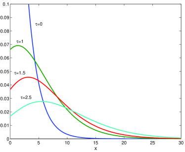
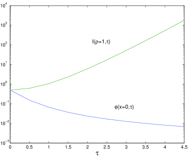
Figure 19: Plot of $\phi(x,\tau)=e^{-\mbox{\small$\frac{1}{2}$}x}\,e^{-4\ln 2\,\tau}I(e^{-x},\tau)$ solution of (43) with initial condition $I(\rho,0)=\mbox{\small$\frac{1}{2}$}\rho$.

From (47) and from the upper plot of Fig. 19, one has that the inclusive distribution vanishes at the non-physical point $x=-x_{0}$ which is slowly varying with $\tau$. The asymptotic shape is developed already at relatively small $\tau$. At $x=0$, corresponding to the physical value $\rho=1$ for $e^{+}e^{-}$ in center of mass, the function $\phi(x,\tau)$ is decreasing, however, thanks to the $e^{4\ln 2\tau}$ factor the inclusive distribution $I(\rho=1,\tau)$ is increasing as shown in the lower plot of Fig. 19.

4.2 Away-from-jet energy flow in $e^{+}e^{-}$

Consider in $e^{+}e^{-}$ annihilation the distribution in the energy emitted outside a cone around the jets, $E_{{\rm out}}$:

$$\Sigma_{e^{+}e^{-}}(E_{{\rm out}})\!=\!\sum_{n}\!\int\frac{d\sigma_{n}}{\sigma_{T}}\,\Theta\!\left(\!E_{{\rm out}}\!-\!\sum_{{\rm out}}q_{ti}\right).$$

This is the simplest (in principle) observable involving non-global single logarithms which were (re)discovered by Mrinal Dasgupta and Gavin Salam Dasgupta:2001sh ; Dasgupta:2002dc ; Dasgupta:2002zf ; Dasgupta:2002bw . These enter all jet-shape observables which involve only a part of phase space and therefore are present in a number of distributions such as: Sterman-Weinberg distribution (energy in a cone); photon isolation; away from jet radiation; rapidity cuts in hadron-hadron (e.g. pedestal); DIS jet in current hemisphere. As for the observable previously discussed, these non-global logs originate from multiple soft gluon emissions at large angles (i.e. not in collinear configuration).

$\Sigma_{e^{+}e^{-}}(E_{{\rm out}})$ contains only single logarithms ($\alpha_{s}^{n}\ln^{n}Q/E_{{\rm out}}$) coming from soft singularities so that $\sigma_{n}/\sigma_{T}$ can be taken as the distribution in the number of soft gluons emitted off the primary $p\bar{p}$ quark-antiquark pair which is known Bassetto:1984ik in the large $N_{c}$ limit. $\Sigma_{e^{+}e^{-}}(E_{{\rm out}})$ was first studied Dasgupta:2001sh ; Dasgupta:2002dc ; Dasgupta:2002zf ; Dasgupta:2002bw numerically by a Monte Carlo method and then studied Banfi:2002hw analytically by deriving the following evolution equation

$$\begin{split}\partial_{\tau}\Sigma_{ab}&=-(\partial_{\tau}R_{ab})\,\Sigma_{ab}\!+\!\int_{{\rm in}}\frac{d\Omega_{q}}{4\pi}\,w_{ab}(q)\left[\Sigma_{aq}\cdot\Sigma_{qb}-\Sigma_{ab}\right],\\ R_{ab}&=\tau\int_{{\rm out}}\!\frac{d\Omega_{q}}{4\pi}\,w_{ab}(q)\,,\end{split}$$ (48)

where $\tau$ is the single logarithmic variable previously introduced (41). As before, to set up a recurrence relation, one needs to generalize the problem by introducing distribution $\Sigma_{ab}=\Sigma_{ab}(E_{{\rm out}})$ for the emission off $ab$-dipole forming an angle $\theta_{ab}$. The physical distribution $\Sigma_{e^{+}e^{-}}(E_{{\rm out}})$ for $e^{+}e^{-}$ in the center of mass is obtained by setting $\theta_{ab}=\pi$.

As shown in (48), the dipole directions $a$ and $b$ are always inside the jet region ($q$ in the integral is bounded inside the jet region). If $a,b$ are in opposite semicones, then either $a,q$ or $q,b$ are in the same semicone. There are many properties of this jet-physics equation (see Dasgupta:2001sh ; Dasgupta:2002dc ; Dasgupta:2002zf ; Dasgupta:2002bw and Banfi:2002hw ). What concerns us here as far as the connection with high-energy physics is the case in which $a,b$ are in the same semicone and we consider $a$ very close to $b$. In the small angle limit we introduce the $2$-dimensional variable $\vec{\theta}$ for the $ab$-dipole ($\Sigma_{ab}\to\Sigma(\vec{\theta})$). For small $\theta$ we can neglect the linear term ($R_{ab}\sim\vec{\theta}^{2}$) so that the evolution equation (48) becomes

$$\begin{split}\partial_{\tau}\Sigma(\tau,\vec{\theta})\!=\!\int&\frac{d^{2}\theta^{\prime}}{2\pi}\frac{\theta^{2}}{{\theta^{\prime}}^{2}(\vec{\theta}\!-\!\vec{\theta^{\prime}})^{2}}\\ &\Big{[}\Sigma(\tau,\vec{\theta^{\prime}})\Sigma(\tau,\vec{\theta}\!-\!\vec{\theta^{\prime}})-\Sigma(\tau,\vec{\theta})\Big{]}\,,\end{split}$$ (49)

with $\vec{\theta}^{\prime}$ ranging in the full plane. The initial condition is $\Sigma(0,\vec{\theta})=1$. This equation is formally the same as the Kovchegov equation Kovchegov:1999yj for the S-matrix

$$\begin{split}\partial_{\tau}S(\tau,\vec{b})=\int&\frac{d^{2}b^{\prime}}{2\pi}\frac{b^{2}}{{b^{\prime}}^{2}(\vec{b}\!-\!\vec{b^{\prime}})^{2}}\\ &\Big{[}S(\tau,\vec{b^{\prime}})S(\tau,\vec{b}\!-\!\vec{b^{\prime}})-S(\tau,\vec{b})\Big{]},\end{split}$$ (50)

where $\vec{b}$ is the impact parameter ranging in the full plane and $\tau={\bar{\alpha}}_{s}Y$ as before. Here the initial condition is $1\!-\!S(0,\vec{b})\sim\alpha_{s}^{2}$ corresponding to the two gluon exchange.

The asymptotic properties of the solutions are well known. Both solutions undergo well known saturation for the variable $\theta^{2}$ or $b^{2}$ larger than a critical value with asymptotic behavior $e^{-c\tau}$ with $c\simeq 4.88\cdots$ determined from the BFKL characteristic function. Beyond such a critical value the solution decreases in $\tau$ as a Gaussian, $\Sigma\sim S\sim e^{-c\tau^{2}/2}$.

The difference in the initial condition makes a difference in the way the saturation regime is asymptotically reached in the two cases. In the high-energy case ($1\!-\!S(0,\vec{b})\sim\alpha_{s}^{2}$) the saturation regime is reached after a critical time $\tau_{c}\sim\ln\alpha_{s}^{-2}/4\ln 2$. In the jet-physics case ($\Sigma(0,\vec{\theta})=1$) there is not a critical $\tau$ and the solution goes without impediment into the saturation regime.

In addition to the different initial conditions, an important difference is that the variables in (48) are angular variables ranging in compact regions. We have seen in the previous analysis that even at small angle it is not fully correct to neglect the compactness affecting the integration limits. This question will be further studied Onofri:2005XX .

4.3 Physics differences

The basis for the two classes of equations, (43),(48) in jet-physics and (44),(50) in high-energy scattering, is of course the (same) multi-soft gluon-distribution. However the dominant contributions for the two classes of observables ($I_{ab},\Sigma_{ab}$ and $T,S$) are obtained from very different kinematical configurations as we discuss now.

Jet-physics case: Here all angles $\theta_{i}$ of emitted gluons are of same order. This is due to the fact that this observable does not contain collinear singularities for $\theta_{ij}\to 0$. Moreover, in the (leading) infrared limit soft gluon energies can be taken ordered so that also the emitted transverse momenta $q_{ti}$ are ordered. The ordered variables $q_{ti}$ enter the argument of the running coupling. The distribution $I_{ab}$ or $\Sigma_{ab}$ are functions of the angular variable $\theta_{ab}$ (which ranges in a compact region) and $\tau$, the logarithmic integral of the running coupling in (41). We are then interested in the solution for finite $\theta_{ab}$ (e.g. $\theta_{ab}=\pi$ in $e^{+}e^{-}$ center of mass) and for $\tau$ never too large.

High-energy scattering case: Here all intermediate soft gluon transverse momenta $q_{ti}$ are of same order (no singularities for vanishing transverse momentum differences). On the other hand, energy ordering implies in this case that intermediate gluon angles $\theta_{i}$ are ordered. Contrary to the previous case, the running coupling is a function of the variables $q_{ti}$ which all are of same order. Therefore, in first approximation, one can take $\alpha_{s}$ fixed. The high-energy $S$-matrix is a function of the impact parameter (which has no bound at large $b$) and $\tau={\bar{\alpha}}_{s}\,Y$. In this case we are then interested in the solution for small $\rho$ (the short distance region) and for $\tau$ large.

As discussed in section 4.1, the fact that the variable $\rho$ entering the jet-observable ranges in a compact region affects the prefactor of the asymptotic behavior and the shape of the distribution at finite angles. In the non linear case discussed in section 4.2, even neglecting compactness at small angle, the difference in the initial conditions affects the ranges in $\tau$ at which the asymptotic behavior (saturation) is developing.

Concluding, by exploiting similarities and differences in the dynamics of high energy scattering and jet-physics (with non-global logs) one hopes that new insights in both fields could be developed.

5 Saturation

Main authors M. Lublinsky and K. Kutak

A parton evolution equation which attempts to describe saturation phenomena was originally proposed by Gribov, Levin and Ryskin Gribov:1984tu (GLR equation) in momentum space and proven in the double log approximation of perturbative QCD by Mueller and Qiu Mueller:1985wy . In the leading $\ln 1/x$ approximation it was derived by Balitsky in the Wilson Loop Operator Expansion Balitsky:1995ub . In the form presented later it was obtained by Kovchegov Kovchegov:1999yj (now called the Balitsky-Kovchegov, or BK equation) in the color dipole approach Mueller:1993rr to high energy scattering in QCD. This equation was also obtained by summation of the BFKL pomeron fan diagrams by Braun Braun:2000wr and most recently Bartels, Lipatov, and Vacca Bartels:2004ef . In the framework of Color Glass Condensate it was obtained by Iancu, Leonidov and McLerran Iancu:2000hn .

5.1 Basic facts about the BK equation

Because the transverse coordinates are unchanged in a high energy collision, unitarity constraints are generally more easy to take into account in a formalism based on the transverse coordinate space representation, and several suggestions for how to include saturation effects in such a formalism have been proposed. Golec–Biernat and Wüsthoff Golec-Biernat:1998js formulated a dipole model, in which a virtual photon is treated as a $q\bar{q}$ or $q\bar{q}g$ system impinging on a proton, and this approach has been further developed by several authors (see e.g. Forshaw:1999uf and Bartels:2002cj ). Mueller Mueller:1993rr ; Mueller:1994jq ; Mueller:1994gb has formulated a dipole cascade model in transverse coordinate space, which reproduces the BFKL equation, and in which it is also possible to account for multiple sub-collisions. Within this formalism Balitsky and Kovchegov Balitsky:1995ub ; Kovchegov:1999yj have derived a non-linear evolution equation (BK equation), which also takes into account these saturation effects from multi-pomeron exchange and which is the best presently available tool to study saturation phenomena at high energies. Contrary to many models the BK equation has solid grounds in perturbative QCD. The equation reads

$$\begin{split}&\frac{d\,N({\mathbf{x}_{01}},y;b)}{d\,y}\,=\,\,\frac{N_{c}\,\alpha_{s}}{2\pi}\,\,\int_{\rho}\,d^{2}{\mathbf{x}_{2}}\frac{{\mathbf{x}^{2}_{01}}}{{\mathbf{x}^{2}_{02}}\,{\mathbf{x}^{2}_{12}}}\,\,\times\\ &\hskip 14.22636pt\left(\,2\,N({\mathbf{x}_{02}},y;{\mathbf{b}-\frac{1}{2}\mathbf{x}_{12}})-\,N({\mathbf{x}_{01}},y;\mathbf{b})\right.\\ &\hskip 19.91684pt\left.-N({\mathbf{x}_{02}},y;{\mathbf{b}-\frac{1}{2}\mathbf{x}_{12}})N({\mathbf{x}_{12}},y;{\mathbf{b}-\frac{1}{2}\mathbf{x}_{02}})\right)\end{split}$$ (51)

The function $N(r_{\perp},x;b)$ is the imaginary part of the amplitude for a dipole of size $r_{\perp}$ elastically scattered at an impact parameter $b$.

In the equation (51), the rapidity $y\equiv-\ln x$. The ultraviolet cutoff $\rho$ is needed to regularize the integral, but it does not appear in physical quantities. We also use the large $N_{c}$ limit (number of colors) value of $C_{F}=N_{c}/2$.

Eq. (51) has a very simple meaning: The dipole of size $\mathbf{x}_{01}$ decays in two dipoles of sizes $\mathbf{x}_{12}$ and $\mathbf{x}_{02}$ with the decay probability given by the wave function $|\Psi|^{2}\,=\,\frac{\mathbf{x}^{2}_{01}}{\mathbf{x}^{2}_{02}\,\mathbf{x}^{2}_{12}}$. These two dipoles then interact with the target. The non-linear term takes into account a simultaneous interaction of two produced dipoles with the target. The linear part of eq. (51) is the LO BFKL equation Kuraev:1977fs ; Balitsky:1978ic , which describes the evolution of the multiplicity of the fixed size color dipoles with respect to the energy $y$. For the discussion below we introduce a short notation for eq. (51):

$$\frac{d\,N}{d\,y}\,\,=\,\alpha_{s}\,\,\mbox{{Ker}}\,\,\otimes\,\,(\,N\,\,-\,\,N\,\,N)\,.$$ (52)

The BK equation has been studied both analytically Kovchegov:1999ua ; Levin:1999mw ; Levin:2000mv ; Kovner:2001bh ; Iancu:2002tr ; Munier:2003sj ; Munier:2003vc and numerically Braun:2000wr ; Gotsman:2002yy ; Armesto:2001fa ; Golec-Biernat:2001if ; Lublinsky:2001yi ; Rummukainen:2003ns ; Golec-Biernat:2003ym ; Gotsman:2004ra . The theoretical success associated with the BK equation is based on the following facts:

• The BK equation is based on the correct high energy dynamics which is taken into account via the LO BFKL evolution kernel.

• The BK equation restores the $s$-channel unitarity of partial waves (fixed impact parameter) which is badly violated by the linear BFKL evolution.

• The BK equation describes gluon saturation, a phenomenon expected at high energies.

• The BK equation resolves the infrared diffusion problem associated with the linear BFKL evolution. This means that the equation is much more stable with respect to possible corrections coming from the non-perturbative domain.

• The BK equation has met with phenomenological successes when confronted against DIS data from HERA Gotsman:2002yy ; Lublinsky:2001yi ; Gotsman:2003br ; Bartels:2003aa ; Bartels:2002uf ; Levin:2001et ; Levin:2001yv ; Lublinsky:2001bc ; Iancu:2003ge .

The BK equation is not exact and has been derived in several approximations.

• The LO BFKL kernel is obtained in the leading soft gluon emission approximation and at fixed $\alpha_{s}$.

• The large $N_{c}$ limit is used in order to express the nonlinear term as a product of two functions $N$. This limit is in the foundation of the color dipole picture. To a large extent the large $N_{c}$ limit is equivalent to a mean field theory without dipole correlations.

• The BK equation assumes no target correlations. Contrary to the large $N_{c}$ limit, which is a controllable approximation within perturbative QCD, the absence of target correlations is of pure non-perturbative nature. This assumption is motivated for asymptotically heavy nuclei, but it is likely not to be valid for proton or realistic nucleus targets.

There are several quite serious theoretical problems which need to be resolved in the future.

• The BK equation is not symmetric with respect to target and projectile. While the latter is assumed to be small and perturbative, the former is treated as a large non-perturbative object. The fan structure of the diagrams summed by the BK equation violates the $t$-channel unitarity. The $t$-channel unitarity is a completeness relation in the $t$-crossing channel. It basically reflects a projectile-target symmetry of the Feynman diagrams. The down-type fan graphs summed by the BK equation, obviously violate the symmetry. A first step towards restoration of the $t$-channel unitarity would be an inclusion of Pomeron loops.

• Though the BK equation respects the $s$-channel unitarity the exchange of massless gluons implies that it violates the Froissart bound for the energy dependence of the total cross section. In order to respect the Froissart bound, gluon saturation and confinement are needed. On one hand, the BK equation provides gluon saturation at fixed and large impact parameters. On the other hand, being purely perturbative, it cannot generate the mass gap needed to ensure a fast convergence of the integration over the impact parameter $b$. Because of this problem, up to now all the phenomenological applications of the BK equation were based on model assumptions regarding the $b$-dependence. It is always assumed that the $b$-dependence factorizes and in practice the BK equation is usually solved without any trace of $b$. At the end, the $b$-dependence is restored via an ansatz with a typically exponential or Gaussian profile. An attempt to go beyond this approximation has been reported in Ref. Golec-Biernat:2003ym ; Gotsman:2004ra .

• It is very desirable to go beyond the BK equation and relax all underlying assumptions outlined above. The higher order corrections are most needed. In particular it is important to learn how to include the running of $\alpha_{s}$, though in the phenomenological applications the running of $\alpha_{s}$ is usually implemented.

• The LO BFKL kernel does not have the correct short distance limit responsible for the Bjorken scaling violation. As a result the BK equation does not naturally match with the DGLAP equation. Though several approaches for unification of the BK equation and DGLAP equations were proposed Kwiecinski:1997ee ; Lublinsky:2001yi ; Gotsman:2002yy ; Kimber:2001nm ; Kutak:2003bd , the methods are not fully developed. All approaches deal only with low $x$ and only with the gluon sector. We would like to have a unified evolution scheme for both small and large $x$ and with quarks included.

5.2 Phenomenology with the BK equation

The deep inelastic structure function $F_{2}$ is related to the dipole amplitude $N$ via

$$\begin{split}F_{2}(x,Q^{2})&=\\ \frac{Q^{2}}{4\pi^{2}}&\int d^{2}r_{\perp}\int dzP^{\gamma^{*}}(Q^{2};r_{\perp},z)\sigma_{\rm dipole}(r_{\perp},x),\end{split}$$ (53)

with the dipole cross section given by the integration over the impact parameter:

$$\sigma_{\rm dipole}(r_{\perp},x)\,\,=\,\,2\,\,\int\,d^{2}b\,N(r_{\perp},x;b).$$ (54)

The physical interpretation of eq. (53) is transparent. It describes the two stages of DIS Gribov:1968gs . The first stage is the decay of a virtual photon into a colorless dipole ($q\bar{q}$ -pair). The probability of this decay is given by $P^{\gamma^{*}}$ known from QED Mueller:1993rr ; Mueller:1989st ; Nikolaev:1990ja ; Levin:1996vf . The second stage is the interaction of the dipole with the target ($\sigma_{\rm dipole}$ in eq. (53)). In the large $N_{c}$ limit a color charge has a well-defined anti-charge partner in a color dipole. Eq. (53) illustrates the fact that in this limit these color dipoles are the relevant degrees of freedom in QCD at high energies Mueller:1993rr .

For the phenomenological applications one may use the function $N(r_{\perp},x;b)$ or $\sigma_{\rm dipole}(r_{\perp},x)$ obtained directly from the solutions of the BK equation (51). With additional DGLAP corrections this approach was adopted by Gotsman et al. in Ref. Gotsman:2002yy .

Alternatively one can relate $N$ to an unintegrated gluon distribution function ${\cal F}(x,k^{2})={f}(x,k^{2})/k^{2}$. The dipole cross section can be expressed via ${f}$ Barone:1993sy ; Bialas:2000xs :

$$\begin{split}\sigma_{\rm dipole}(r_{\perp},x)&=\\ \frac{8\,\pi^{2}}{N_{c}}&\int\frac{d\,k^{2}}{k^{4}}\,\left[1\,-\,J_{0}(k\,r_{\perp})\right]\,\alpha_{s}(k^{2})\,{f}(x,k^{2})\end{split}$$ (55)

The inversion of eq. (55) is straightforward

$${f}(x,k^{2})\,=\,\int d^{2}b\,h(k^{2},x,b),$$ (56)

$$\begin{split}h(k^{2},x,b)\,&=\,\frac{N_{c}}{4\,\alpha_{s}\,\pi^{2}}\,k^{4}\,\Delta_{k}\,\tilde{N}(k^{2},x,b)\\ &=\,\frac{N_{c}}{\alpha_{s}\,\pi^{2}}\,\frac{k^{2}\,\partial^{2}}{\partial\,(\ln k^{2})^{2}}\,\tilde{N}(k^{2},x,b)\,.\end{split}$$ (57)

Here $\Delta_{k}$ is the 2-dimensional Laplace operator. The function $\tilde{N}$ is related to the Fourier transform of $N$

$$\tilde{N}(k^{2},x,b)\,=\,\int\frac{d^{2}\,\mathbf{r}_{\perp}}{2\,\pi\,r_{\perp}^{2}}\,e^{\,i\,\mathbf{k}\,\mathbf{r}_{\perp}}\,N(r_{\perp},x,b)\,.$$ (58)

In fact, $\tilde{N}$ obeys a nonlinear version of the LO BFKL evolution equation in momentum space. The function $\tilde{N}$ can be interpreted as an unintegrated gluon distribution. $\tilde{N}$ and $h$ coincide at large momenta but differ at small ones. On one hand, within the dipole picture it is rather the function $\tilde{N}$ which gives the probability to find a gluon with a given transverse momentum and at a given impact parameter. On the other hand, it is the function ${f}$ (or $h$) which enters the $k_{\perp}$ (high energy) factorization formula. In what follows we will concentrate on the unintegrated gluon distribution ${f}$ only.

Instead of solving the BK equation (51) and then inverting the relation (55) one can adopt another strategy and reformulate the problem directly in terms of the unintegrated gluon density ${f}$. This approach was adopted in work by Kutak-Kwiecinski Kutak:2003bd and Kutak-Stasto Kutak:2004ym . Using relations (54) and (55) one can transform (51) into an equation for the unintegrated gluon distribution

$$\begin{split}{f}(x,&k^{2})=\tilde{f}^{(0)}(x,k^{2})\\ +&\,\frac{N_{c}\alpha_{s}(k^{2})}{\pi}k^{2}\int_{x}^{1}\frac{dz}{z}\int_{k_{0}^{2}}\frac{dk^{\prime 2}}{k^{\prime 2}}\\ &\bigg{\{}\frac{{f}(\frac{x}{z},k^{\prime 2})\,-\,{f}(\frac{x}{z},k^{2})}{|k^{\prime 2}-k^{2}|}+\frac{{f}(\frac{x}{z},k^{2})}{|4k^{\prime 4}+k^{4}|^{\frac{1}{2}}}\,\bigg{\}}\,\\ -&\left(1-k^{2}\frac{d}{dk^{2}}\right)^{2}\frac{k^{2}}{R^{2}}\int_{x}^{1}\frac{dz}{z}\\ &\left[\int_{k^{2}}^{\infty}{dk^{\prime 2}\,k^{\prime 4}}\alpha_{s}(k^{\prime 2})\ln\left({k^{\prime 2}k^{2}}\right){f}(z,k^{\prime 2})\right]^{2}.\end{split}$$ (59)

Here it is written as an integral equation, corresponding to the BFKL equation in momentum space supplemented by the negative nonlinear term. The input $\tilde{f}^{(0)}(x,k^{2})$ is given at the scale $k_{0}^{2}=1GeV^{2}$. This equation was derived under the following factorization ansatz:

$$\tilde{N}(k^{2},x,b)=\tilde{n}(k^{2},l,x)\,S(b)$$ (60)

with normalization conditions on the profile function $S(b)$

$$\int d^{2}{\bf b}\,S(b)=1;\qquad\int d^{2}{\bf b}\,S^{2}(b)=\frac{1}{\pi R^{2}}.$$ (61)

The assumption (60) is crude and corresponds to a situation where the projectile size (color dipole) is neglected compared to the target size (proton). A simple way to improve (59) is to implement NLO corrections in the linear term of the equation. It can be done within the unified BFKL-DGLAP framework which is presented below. The final equation (eq. (64) below) can be used for phenomenological applications. Figs. 20, 21 display the unintegrated gluon distributions ${f}$ obtained in Refs. Gotsman:2002yy ; Kutak:2004ym .

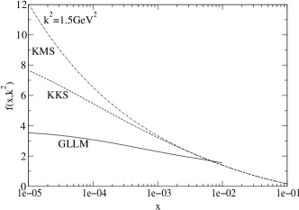
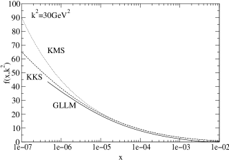
Figure 20: The unintegrated gluon distribution ${f}(x,k^{2})$ as a function of $x$ for different values $k^{2}=1.5\,GeV^{2}$ (top) and $k^{2}=30\,GeV^{2}$ (bottom). Solid lines correspond to the solution of the nonlinear equation using GLLM Gotsman:2002yy parameterization whereas dashed lines (KKS) correspond to the approximate solution of (64)Kutak:2003bd ; Kutak:2004ym . For reference we also present linear BFKL/DGLAP evolution (KMS)Kwiecinski:1997ee .

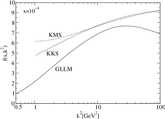
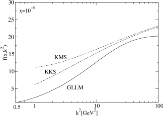
Figure 21: The unintegrated gluon distribution ${f}(x,k^{2})$ as a function of $k^{2}$ for different values $x=10^{-4}$ (left) and $x=10^{-5}$ (right). The lines are the same as in fig. 20 .

5.3 The saturation scale

In order to quantify the strength of effects that slow down the gluon evolution one introduces the saturation scale $Q_{s}(x)$. It divides the $(x,k^{2})$-space into regions of dilute and dense partonic systems. In the case when $k^{2}\,<\,Q_{s}^{2}(x)$ the solution of the BK equation exhibits geometrical scaling, which means that it depends on one variable only, $N(r,x)=N(r\,Q_{s}(x))$ or in momentum space $\tilde{N}(k^{2},x)=\tilde{N}(k/Q_{s}(x))$. In Fig. 22 we present saturation scales obtained from (59) in Kutak:2004ym and the corresponding result obtained from Ref. Gotsman:2002yy . Note, however, that the saturation scale is defined differently in these two approaches. In ref. Kutak:2004ym the saturation scale is defined quantitatively as a relative difference between the solutions to the linear and nonlinear equations, while in ref. Gotsman:2002yy it is defined by the requirement that $N(2/Q_{s},x)$ is constant equal to $1/2$ or $1/e$. Note that both the KKS Kutak:2004ym and the GLLM models predict a saturation scale much bigger than the one from the GBW model.

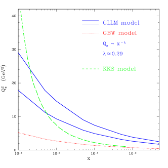
Figure 22: Saturation scale from various models. The solid lines defines a band of possible saturation scales coming from the GLLM model Gotsman:2002yy . The dashed line (KKS) is from Ref. Kutak:2004ym . The dotted line (GBW) is the Golec-Biernat Wüsthoff model Golec-Biernat:1998js .

5.4 Beyond the BK equation

Saturation effects are most easily studied in the coordinate space representation in which it has been difficult to include non-leading effects, and the non-leading effects have mainly been studied in momentum space, where it is hard to include saturation. We now present a short (not complete) review of recent theoretical activities which attempt to go beyond the leading order BK equation. An important issue relating to the NLO corrections is energy–momentum conservation, which was already addressed in section 2.2 and will be further discussed in more detail in section 5.5.

5.4.1 Beyond leading order

The BFKL kernel is known at next-to-leading order. Nevertheless, a nonlinear equation at NLO has not been derived yet. I. Balitsky and A. Belitsky Balitsky:2001mr have been able to compute a single NLO contribution which has maximal nonlinearity, namely the $N^{3}$ term:

$$\frac{d\,N}{d\,y}=\alpha_{s}\mbox{{Ker}}\otimes(N-N\cdot N)-\alpha_{s}^{2}\overline{\mbox{{Ker}}}\otimes N\cdot N\cdot N.$$ (62)

The new kernel $\overline{\mbox{{Ker}}}$ can be found in Ref Balitsky:2001mr . Triantafyllopoulos Triantafyllopoulos:2002nz has considered NLO BFKL in the presence of a saturation boundary. The results show a decrease in the saturation scale growth as a function of rapidity towards the value $\lambda\,\simeq\,0.3$ observed experimentally (GBW Golec-Biernat:1998js and GLLM Gotsman:2002yy models).

Another approach Kimber:2001nm ; Kutak:2003bd to partially include the NLO corrections into the BK equation is to implement in the linear term of eq. (59) the unified BFKL-DGLAP framework developed in Kwiecinski:1997ee . In this scheme the BFKL kernel also gets modified by the consistency constraint Andersson:1995jt ; Kwiecinski:1996td ; Ciafaloni:1988ur

$$k^{\prime 2}<k^{2}/z.$$ (63)

The origin of this constraint is the requirement that the virtuality of the exchanged gluon is dominated by its transverse momentum $|k^{\prime 2}|\simeq k_{T}^{\prime 2}$ (see also section 2.2). The constraint (63) resums a large part of the subleading corrections in $\ln 1/x$, and it is also connected to the conservation of the negative lightcone component $p_{-}=E-p_{L}$ (cf. section 5.5). Additionally, the non-singular part of the leading order DGLAP splitting function, which influences the normalization of the unintegrated gluon distribution, is included into the evolution and $\alpha_{s}$ is assumed to run with the scale $k^{2}$ . The final improved nonlinear equation for the unintegrated gluon density becomes

$$\begin{split}&{f}(x,k^{2})\;=\;\tilde{f}^{(0)}(x,k^{2})+\\ &+\,\frac{N_{c}\alpha_{s}(k^{2})}{\pi}k^{2}\int_{x}^{1}\frac{dz}{z}\int_{k_{0}^{2}}\frac{dk^{\prime 2}}{k^{\prime 2}}\,\\ &\bigg{\{}\,\frac{{f}(\frac{x}{z},k^{\prime 2})\,\Theta(\frac{k^{2}}{z}-k^{\prime 2})\,-\,{f}(\frac{x}{z},k^{2})}{|k^{\prime 2}-k^{2}|}+\,\frac{{f}(\frac{x}{z},k^{2})}{|4k^{\prime 4}+k^{4}|^{\frac{1}{2}}}\,\bigg{\}}\\ &+\,\frac{\alpha_{s}(k^{2})}{2\pi}\int_{x}^{1}dz\,\bar{P}_{gg}(z)\int^{k^{2}}_{k_{0}^{2}}\frac{dk^{\prime 2}}{k^{\prime 2}}\,{f}(\frac{x}{z},k^{\prime 2})\\ &-\left(1-k^{2}{d\over dk^{2}}\right)^{2}{k^{2}\over R^{2}}\int_{x}^{1}\frac{dz}{z}\\ &\hskip 28.45274pt\left[\int_{k^{2}}^{\infty}{dk^{\prime 2}\over k^{\prime 4}}\alpha_{s}(k^{\prime 2})\ln\left({k^{\prime 2}\over k^{2}}\right){f}(z,k^{\prime 2})\right]^{2}\;,\end{split}$$ (64)

with the input distribution $\tilde{f}^{(0)}(x,k^{2})$.

5.4.2 JIMWLK

The $N_{c}$ corrections can be accounted for through the JIMWLK functional equation Jalilian-Marian:1996xn ; Jalilian-Marian:1997dw ; Jalilian-Marian:1998cb ; Kovner:2000pt ; Weigert:2000gi , which is equivalent to Balitsky’s original infinite chain of equations Balitsky:1995ub . Introducing $N$ as a target expectation value of a certain operator (product of two Wilson lines), $N\,\,\equiv\,\,\langle\,W\,\rangle_{target}$, the first couple of equations of the Balitsky chain are

$$\hskip 28.45274pt\frac{d\,\langle\,W\,\rangle}{d\,y}\,\,=\,\alpha_{s}\,\mbox{{Ker}}\,\otimes\,(\,\langle\,W\,\rangle\,\,-\,\,\langle\,W\,W\,\rangle),$$ (65)

$$\frac{d\,\langle\,W\,W\,\rangle}{d\,y}\,=\alpha_{s}\,\mbox{{Ker}}\,\otimes\,(\langle\,W\,W\,\rangle\,-\,\langle\,W\,W\,W\,\rangle).$$ (66)

The large $N_{c}$ limit and the absence of the target correlations used by Kovchegov Kovchegov:1999yj is equivalent to a mean field approximation which allows to express a correlator of a product as a product of correlators:

$$\langle\,W\,W\,\rangle\,\,=\,\,\langle\,W\,\rangle\,\langle\,W\,\rangle\,\,=\,\,N\,N\,;\,\,N_{c}\,\rightarrow\,\infty.$$

Thus the first equation of the Balitsky chain closes to the BK equation.

Rummukainen and Weigert Rummukainen:2003ns have produced a first numerical solution of the JIMWLK equation. They do not find any qualitative deviation from solutions of the BK equation. The $N_{c}$ corrections were found to be at a level of a few percents.

Bartels, Lipatov, and Vacca Bartels:2004ef have considered $N_{c}$ corrections to the triple Pomeron vertex:

$$\hskip 28.45274pt\frac{d\,N}{d\,y}\,\,=\,\alpha_{s}\,\,\mbox{{Ker}}\,\,\otimes\,\,(\,N\,\,-\,\,N\,\,N\,\,-\,\,{\frac{1}{N_{c}^{2}}\,n})\,$$

where the function $n$ has to satisfy a separate equation.

5.4.3 Target correlations

For proton and realistic (not very dense) nucleus targets a systematic approach towards inclusion of target correlations has been developed by Levin and Lublinsky Levin:2003nc . Target correlations can be introduced via a certain linear functional differential equation. In general, this linear functional equation cannot be reformulated as a non-linear equation. However, in a particular case when all $n$-dipole correlations can be accounted for by a single correlation parameter, the equation can be brought to a modified version of the BK equation:

$$\frac{d\,N}{d\,y}\,=\,\alpha_{s}\,\mbox{{Ker}}\,\otimes\,(\,N\,-\,\kappa\,N\,N);$$ (67)

In Eq. (67) $\kappa\geq 1$ is the correlation parameter to be found from a model for the target.

5.4.4 Pomeron loops

Pomeron loops are the first steps towards restoration of the $t$-channel unitarity. Iancu and Mueller Iancu:2003zr have considered rare fluctuations which were interpreted by Kozlov and Levin Kozlov:2004sh as pomeron loop contributions. Unfortunately, it looks as if contributions from the pomeron loops are difficult to incorporate in a framework of a single equation. They are known to modify the asymptotic behavior of the amplitude $N$ in the deep saturation limit, where they give the following asymptotic behavior:

$$N(Y)\,\,=\,\,1\,\,-\,\,e^{\,-\,c\,(Y\,-\,Y_{0})^{2}};\quad Y\,\rightarrow\,\infty\quad c\,=\,2\,\bar{\alpha}_{s}\quad\mbox{BKE}$$

$$N(Y)\,\,=\,\,1\,\,-\,\,e^{\,-\,c\,(Y\,-\,Y_{0})^{2}/2};\quad Y\,\rightarrow\,\infty\quad Pom\,\,Loops$$

Recently there has been a lot of activity in attempting to consistently include Pomeron loops into high energy evolutions Iancu:2004iy ; Mueller:2005ut ; Levin:2005au ; Kovner:2005nq ; Kovner:2005jc ; Kovner:2005en .

5.4.5 Local multi-pomeron exchange

It is claimed that the BK equation sums all possible contributions which are not suppressed either by $\alpha_{s}$ or $N_{c}$. For example, the cubic term in Eq. (62) appears at next-to-leading $\alpha_{s}$ order only. In particular it is implied that all multi-pomeron exchanges and multi-pomeron vertices are either absorbed by the triple pomeron vertex of the BK equation or suppressed. Levin and Lublinsky Levin:2003nc have argued that this might be not true. They argue that in addition to a possibility for a pomeron to split into two, there exists a process of multi-pomeron exchange, which is local in rapidity. After these contributions were resummed in the eikonal approximation, a new modification of the BK equation was proposed:

$$\frac{d\,N}{d\,y}\,\,=\,\,(1\,\,-\,\,N)\,\alpha_{s}\,\,\mbox{{Ker}}\,\,\otimes\,\,(\,N\,\,-\,\,N\,\,N).$$ (68)

5.5 Energy conservation aspects

Main author G. Gustafson

5.5.1 Rapidity veto

It is well known Salam:1999cn that a major fraction of the higher order corrections to (not only) BFKL is related to energy conservation. The large effect of energy-momentum conservation is also clearly demonstrated by the numerical analyses by Andersen-Stirling Andersen:2003gs and Orr-Stirling Orr:1997im . Conservation of energy and momentum implies the conservation of both the positive and the negative lightcone components, $p_{\pm}=E\pm p_{L}$. Although most analyses have concentrated on the conservation of $p_{+}$, as being more important, we will see below that also conservation of $p_{-}$ has a very significant effect. In LLA the steps in $\ln(1/x)$ are assumed to be large, and the necessary recoils due to energy conservation are neglected. The main effect of conservation of the positive lightcone component $p_{+}=E+p_{L}$, is that small steps in $\ln(1/x)$ with corresponding large recoils are suppressed. One way to take this into account is to introduce a veto, not allowing steps in $\ln(1/x)$ smaller than a cut $\eta$. (This is called a rapidity veto also if the evolution variable is defined as $y=\ln(1/x)$ and not the true rapidity.) The effect of such a veto is studied in refs. Andersson:1996ju ; Schmidt:1999mz ; Forshaw:1999xm , and at high energies it has a similar effect as the higher order corrections, reducing the growth at small $x$.

A recent study of the BK equation in the presence of a rapidity veto is presented by Chachamis, Lublinsky and Sabio Vera Chachamis:2004ab . The application of this method to the BK equation makes it non-local in rapidity:

$$\frac{d\,N(y)}{d\,y}\,\,=\,\alpha_{s}\,Ker\,\,\otimes\,\,(\,N(y\,{-\,\eta})\,\,-\,\,N(y\,{-\,\eta})\,\,N(y\,{-\,\eta}))\,.$$

The veto somewhat delays saturation in accordance with the expectations associated with the next-to-leading order corrections. If the veto is put on top of the BK equation with running $\alpha_{s}$ then the effect of NLO corrections is significantly reduced. This observation gives support to the phenomenological studies of Refs. Gotsman:2002yy ; Kutak:2003bd .

An similar approach to this problem is presented by Gotsman, Levin, Maor, and Naftali Gotsman:2005vc . The effects of the cut in $\ln(1/x)$ is taken into account in a modified BK equation:

$$\begin{split}&\frac{\partial N(r,Y;b)}{\partial Y}=\frac{C_{F}\alpha_{s}}{\pi^{2}}\int\frac{d^{2}r^{\prime}r^{2}}{(\mathbf{r}-\mathbf{r^{\prime}})^{2}r^{\prime 2}}\left(1-\frac{\partial}{\partial Y}\right)\\ &\times\left[2N\left(r^{\prime},Y;\mathbf{b}-\frac{1}{2}(\mathbf{r}-\mathbf{r^{\prime}})\right)-N\left(r,Y;\mathbf{b}\right)\right.\\ &\left.\hskip 14.22636pt-N\left(r^{\prime},Y;\mathbf{b}-\frac{1}{2}(\mathbf{r}-\mathbf{r^{\prime}})\right)N\left(\mathbf{r}-\mathbf{r^{\prime}},Y;\mathbf{b}-\frac{1}{2}\mathbf{r^{\prime}}\right)\right].\end{split}$$ (69)

The derivative under the integral is related to a cut in $\ln(1/x)\propto\ln p_{+}$. The modification of the pole at $\gamma=1$, which is related to conservation of the negative lightcone component $p_{-}=E-p_{L}$ (or the inverse $k_{\perp}$ ordering) and the consistency constraint, is not included. The motivation for this is that this effect is not important once the dipole density has reached saturation, that is for $x$ so small that $Q_{s}^{2}(x)>Q^{2}$.

We note, however, that the non-leading effects can significantly reduce the value of $Q_{s}^{2}(x)$, and thus delay the onset of saturation, as discussed in e.g. refs. Triantafyllopoulos:2002nz . An essential result of the analysis discussed in the next subsection is that also the conservation of $p_{-}$ has an important effect, and contributes significantly to pushing the $x$-values, where saturation becomes essential, to smaller values. We note also that an estimate of the relative importance of saturation and non-leading effects for the reduced growth rate is very important for reliable extrapolations to higher energies at LHC and high energy cosmic rays.

5.5.2 Full energy-momentum conservation

A different approach to energy-momentum conservation is presented in ref. Avsar:2005iz . As discussed above non-leading effects are most easily studied in momentum space, while unitarity or saturation effects are easier analyzed when formulated in transverse coordinate space. In ref. Avsar:2005iz similarities between the Linked Dipole Chain model (LDC) Andersson:1996ju ; Andersson:1998bx in momentum space and the Mueller dipoles in transverse coordinate space Mueller:1993rr ; Mueller:1994jq ; Mueller:1994gb are used to derive a scheme for implementing energy momentum conservation in Mueller’s dipole formalism. It is conjectured that only those gluon emissions, which satisfy energy-momentum conservation, can correspond to real final state gluons, and that keeping only these (with a corresponding modification of the Sudakov form factor) will not only give a better description of the final states, but also account for essential parts of the NLO corrections to the BFKL equation. The approach is based on the observation that the emission of a dipole with a very small transverse size, $r$, corresponds to having two very well localized gluons, and such gluons must have large transverse momenta of the order $p_{\perp}\sim 1/r$. By in this way assigning a transverse momentum to each emitted gluon, and also taking into account the recoils of the emitting gluons, it is possible to make sure that each dipole splitting is kinematically allowed.

Figure 23: A quark-antiquark dipole in transverse coordinate space is split into successively more dipoles via gluon emission.

Formalism

In the process $\gamma^{*}\rightarrow Q\bar{Q}\rightarrow Qg\bar{Q}\rightarrow Qgg\bar{Q}\rightarrow\ldots$, a virtual photon is split into a $Q\bar{Q}$ color dipole, which is first split into two dipoles by the emission of a gluon, then into three dipoles by a second gluon, etc. The process is illustrated in transverse coordinate space in fig. 23. The probability for such a dipole splitting is given by the expression Mueller:1993rr ; Mueller:1994jq ; Mueller:1994gb (for notation see fig. 23)

$$\begin{split}\frac{dP}{dy}&=\frac{\bar{\alpha}}{2\pi}d^{2}\textbf{r}_{2}\frac{r_{01}^{2}}{r_{02}^{2}\,r_{12}^{2}}\cdot S;\\ S&=\exp\left[-\frac{\bar{\alpha}}{2\pi}\int dy\int d^{2}\textbf{r}_{2}\frac{r_{01}^{2}}{r_{02}^{2}\,r_{12}^{2}}\right].\end{split}$$ (70)

Here $S$ denotes a Sudakov form factor. We note that the integral over $d^{2}\textbf{r}_{2}$ in the exponent diverges for small values of $r_{02}$ and $r_{12}$. Therefore Mueller introduced a cutoff $\rho$, such that the integration region satisfies $r_{02}>\rho$ and $r_{12}>\rho$. A small cutoff value $\rho$ will here imply that we get very many dipoles with small $r$-values.

If a dipole size, r, is small, it means that the gluons are well localized, which must imply that transverse momenta are correspondingly large. This implies that not only the new gluon gets a large $k_{\perp}\sim 1/r$, also the original gluon, which is close in coordinate space, gets a corresponding recoil. Let us study the example in fig. 24. For the emissions of the gluons marked 2, 3, and 4 the dipole sizes become smaller and smaller, $a\gg b\gg c\gg d$, in each step of the evolution. The corresponding $k_{\perp}$ therefore become larger and larger in each step. After the minimum dipole, with size $d$, the subsequent emissions, 5, and 6, give again larger dipoles with correspondingly lower $k_{\perp}$ values. The probability for this chain is proportional to

$$\frac{d^{2}\textbf{r}_{2}\,a^{2}}{a^{2}\,b^{2}}\cdot\frac{d^{2}\textbf{r}_{3}\,b^{2}}{b^{2}\,c^{2}}\cdot\frac{d^{2}\textbf{r}_{4}\,c^{2}}{c^{2}\,d^{2}}\cdot\frac{d^{2}\textbf{r}_{5}\,d^{2}}{e^{2}\,e^{2}}\cdot\frac{d^{2}\textbf{r}_{6}\,e^{2}}{f^{2}\,f^{2}}$$ (71)

For the first emissions, 2 and 3, in this expression we recognize the product of factors $d^{2}\textbf{r}_{i}/r_{i}^{2}\,\sim\prod d^{2}\textbf{k}_{i}/k_{i}^{2}$, just as is expected from a “DGLAP evolution” of a chain with monotonically increasing $k_{\perp}$. Emission number 4 corresponds to the minimum dipole size, $d$, and we here note that the factors of $d$ cancel in eq. (71). We therefore get the weight $d^{2}\textbf{r}_{4}\sim d^{2}\textbf{k}_{\mathrm{max}}/k_{\mathrm{max}}^{4}$, which corresponds to a hard gluon-gluon collision. When the dipole sizes get larger again, this gives factors corresponding to a “DGLAP chain” from the other end of the chain, up to the central hard subcollision.

Figure 24: A dipole cascade, where a chain of smaller and smaller dipoles is followed by a set of dipoles with increasing sizes. This is interpreted as one $k_{\perp}$-ordered cascade from the left and one from the right, up to a central hard subcollision, which is represented by the dipole with minimum size and therefore maximum $k_{\perp}$.

It is also easy to see that for a chain with increasing dipole sizes up to a maximum value, $r_{\mathrm{max}}$, which thus corresponds to a minimum transverse momentum, $k_{\perp\mathrm{min}}$, we get the weight $d^{2}\textbf{r}_{\mathrm{max}}/r_{\mathrm{max}}^{4}\sim d^{2}\textbf{k}_{\mathrm{min}}$. Therefore there is no singularity for the minimum $k_{\perp}$-value. This result agrees exactly with the result in the Linked Dipole Chain model, LDC Andersson:1996ju ; Andersson:1998bx , which is a reformulation of the CCFM model Catani:1990yc ; Ciafaloni:1988ur , interpolating between DGLAP and BFKL for non-$k_{\perp}$-ordered chains.

Figure 25: A symbolic picture of a $\gamma^{*}\gamma^{*}$ collision in rapidity-$\mathbf{r}_{\perp}$-space. The two dipole chains interact and recouple with probability $f$ given by eq. (72).

To study $\gamma^{*}\gamma^{*}$ scattering we imagine that the two virtual photons split up into quark-antiquark pairs, which develop into dipole cascades as schematically illustrated in fig. 25. When the two central dipoles collide and interact via gluon exchange, it implies a recoupling of the color charges, as indicated by the arrow, and the probability for this is given by the expression Salam:1995uy

$$f=\frac{\alpha_{s}^{2}}{2}\left\{\ln\left[\frac{|\textbf{r}_{1}-\textbf{r}_{3}|\cdot|\textbf{r}_{2}-\textbf{r}_{4}|}{|\textbf{r}_{1}-\textbf{r}_{4}|\cdot|\textbf{r}_{2}-\textbf{r}_{3}|}\right]\right\}^{2}.$$ (72)

As the dipole cascades from the two virtual photons branch out, it is also possible to have multiple collisions, when more than one pair of dipoles from the left and the right moving cascades are interacting. The total cross section is then given by

$$\sigma\sim\int d^{2}b(1-e^{-\sum f_{ij}}),$$ (73)

where $b$ denotes the impact parameter.

With a small cutoff $\rho$ ($r>\rho$) we get, as mentioned above, very many small dipoles. If these are interpreted as real emissions, it would imply a violation of energy-momentum conservation. The emission of these small dipoles must be compensated by virtual emissions. Thus the result in eq. (73) will describe the inclusive cross section, but the many dipoles produced in all the branching chains will not correspond to the production of exclusive final states.

The main feature of the LDC model is the observation that both the total cross section and the final state structures are determined by chains consisting of a subset of the gluons appearing in the final state. These gluons were called “primary gluons” in ref. Andersson:1996ju and later called “backbone gluons” in ref. Salam:1999ft . Remaining real final state gluons can be treated as final state radiation from the primary gluons. Such final state emissions do not modify the total cross sections, and give only small recoils to the parent emitters. The primary gluons have to satisfy energy-momentum conservation, and are ordered in both positive and negative light-cone momentum components, $p_{+}$ and $p_{-}$. We saw above that in Mueller’s cascade the emission probabilities for gluons, which satisfy the conditions for primary gluons in LDC, have exactly the same weight, when the transverse momenta are identified with the inverse dipole size, $2/r$. This inspires the conjecture that with this identification an appropriate subset of the emissions in Mueller’s cascade can correspond to the primary gluons in the momentum space cascade, meaning that they determine the cross sections while the other emissions can be regarded as either virtual fluctuations or final state radiation.

A necessary condition for this subset of gluons is that energy and momentum is conserved. Therefore we expect that keeping only emissions which satisfy energy-momentum conservation can correspond to real emissions, and keeping only these emissions (with a corresponding modification of the Sudakov form factor) will not only account for important NLO effects, but also give a closer correspondence between the generated dipole chains and the observable final states.

A very important consequence of energy-momentum conservation is also that it implies a dynamical cutoff, $\rho(\Delta y)$, which is large for small steps in rapidity, $\Delta y$, but gets smaller for larger $\Delta y$. (Alternatively it could be described as a cutoff for $\Delta y$ which depends on $r$. Note that in this formalism $y$ is the true rapidity and not $\log(1/x)$.) Conserving also the negative light-cone momentum, $p_{-}$, implies that in a similar way we may also get a maximum value for $r$ in each emission.

The net result of conservation of both $p_{+}$ and $p_{-}$ is that the number of dipoles grows much more slowly with energy. Besides its physical effects, this also simplifies the implementation in a MC program. It is here straight forward to calculate cross sections and to study saturation effects, by comparing the unitarized expression $\int d^{2}b(1-e^{-\sum f_{ij}})$ in eq. (73) with $\int d^{2}b\sum f_{ij}$ representing single $I\!\!P$ exchange. (The large numerical complications in MCs without energy conservation, discussed in ref. Salam:1995uy , are not present.)

Results

Below we show some results obtained with a fixed coupling $\bar{\alpha}=0.2$.

Dipole-dipole scattering. The cross section for scattering of two dipoles with sizes $r_{1}$ and $r_{2}$ is shown in fig. 26. With a fixed coupling the scaled cross section, $\sigma/r_{2}^{2}$, depends only on the ratio $r_{1}/r_{2}$. We can imagine a target with size $r_{2}\sim 1/M$, and a varying projectile size $r_{1}\sim 1/\sqrt{Q^{2}}$. The results show that the cross section grows faster with the total rapidity range, $Y\sim\ln s$, for smaller $r_{1}$ (larger $Q^{2}$), in a way qualitatively similar to the behavior of the proton structure function.

Figure 26: The scaled unitarized dipole–dipole cross section, $\sigma/r_{2}^{2}$, as a function of $Y$ for different initial conditions.

Figure 27: The scaled unitarized (full line) and one-pomeron (dashed line) dipole–dipole cross sections calculated without energy conservation.

The effect of energy conservation is demonstrated in fig. 27 by the results obtained for the case $r_{1}\!=\!r_{2}$, with a constant cutoff, $\rho=0.02\,r_{i}$. Comparing with fig. 26 we see that energy conservation has a very strong effect, reducing $\sigma$ by almost an order of magnitude for $Y\sim 13$.

In fig. 27 we also see that without energy-momentum conservation the effect of multiple $I\!\!P$ exchange (saturation) is about a factor 2 for $r_{1}=r_{2}$ and $Y=13$. The much smaller cross section obtained with energy-momentum conservation implies that the saturation effect is much less important, being only $\approx 20\%$ for the same parameter values.

Dipole-nucleus and dipole-proton collisions. Dipole-nucleus collisions have been studied using a toy model nucleus, with a Gaussian distribution in dipole size $r$ and impact parameter $b$. The dipole density is given by

$$dN=B\cdot d^{2}\textbf{r}\,e^{-r^{2}/r_{0}^{2}}\cdot d^{2}\textbf{b}\,e^{-b^{2}/b_{0}^{2}}$$ (74)

The widths of the distributions are taken to be $r_{0}=1\,\mathrm{fm}$ and $b_{0}=A^{1/3}\cdot 1\,\mathrm{fm}$ (where $A$ is the mass number of the nucleus), and the normalization constant $B$ is adjusted so that the transverse energy is given by $A\!\cdot\!1\,\mathrm{GeV}$.

Figure 28: The dipole–nucleus cross section for $r_{\mathrm{proj}}=0.1$ and $1$ GeV^-1 and $A=200$. The unitarized result is shown by the solid lines, and the one-pomeron contribution by the dashed lines.

The results for $A=200$ and projectile sizes $r_{\mathrm{proj}}=0.1$ and $1$ GeV^-1 are shown in figure 28. Results are presented both for single pomeron exchange and including unitarization. The effect of unitarization grows with nuclear size and with the size of the projectile. For a small projectile of size $0.1$ GeV^-1 we can see the effect of color transparency, as the cross sections for the unitarized and the one pomeron calculations are almost identical. For a larger projectile we do see a clear effect from unitarization, but even for $r_{\mathrm{proj}}=1$ GeV^-1 and a nucleus with $A=200$ this effect is only about $20\%$ in the rapidity interval $10-14$. For smaller nuclei the effect will be correspondingly smaller.

When the same toy model is applied to deep inelastic ep scattering (with $A=1$ and simply identifying $Q^{2}$ with $4/r_{\mathrm{proj}}^{2}$), we want to emphasize that we here only want to study the qualitative behavior. A quantitative comparison with HERA data has to wait for an improvement of the crude toy model for the proton target (dipole correlations may be important), and one should then also take into account the detailed effects of the photon wavefunction.

The resulting dipole–nucleon cross section is shown in figure 29 for two different projectile sizes, corresponding to $Q^{2}=4\,\mathrm{GeV}^{2}$ and $Q^{2}=400\,\mathrm{GeV}^{2}$. The result for single pomeron exchange, i.e. without unitarization corrections, is shown by the dashed lines, and we see that the effect from unitarization is quite small.

Figure 29: The scaled dipole–p cross section as a function of log$1/x$, for $Q^{2}=4$ GeV² and $Q^{2}=400$ GeV². The unitarized results are shown by the solid lines while the dashed lines show the one-pomeron results.

In figure 29 we also see that the logarithmic slope $\lambda_{\mathrm{eff}}=d(\log\sigma)/d(\log 1/x)$ is increasing with increasing $Q^{2}$. The effective slope, $\lambda_{\mathrm{eff}}$, is not a constant for fixed $Q^{2}$, but depends on both $Q^{2}$ and $x$, when unitarization and/or energy conservation is taken into account. For the comparison with experimental data figure 30 shows $\lambda_{\mathrm{eff}}$ determined in the $x$-interval used in the analysis by H1 Adloff:2001rw , which varies from $x\approx 2\times 10^{-5}$ for $Q^{2}=1.5$ GeV² to $x\approx 3\times 10^{-2}$ for $Q^{2}=90$ GeV². We note that the result of our crude model is not far from the experimental data, although the dependence on $Q^{2}$ is somewhat weaker in the model calculations. As in figure 29 we see that the effect of unitarization is small, and, as expected, it gets further reduced for larger $Q^{2}$-values.

Figure 30: The effective slope measured at different $Q^{2}$ compared to data from HERA. The full line is our model including unitarization, while the dashed line is without. Filled circles are data from ZEUSBreitweg:2000yn , filledAdloff:2000qk and openDIS04Petrukhin squares are data from H1.

Thus we find that the result of the simple model is surprisingly close to experimental data from HERA. The effect of energy conservation is a suppression for small $x$-values and small $Q^{2}$, which is qualitatively similar to the effect expected from unitarization. This suppression is so strong that the effect from adding unitarization is only a very small correction, visible for small $Q^{2}$-values.

If we compare these results with those of ref. Gotsman:2005vc , we find a significantly larger effect from energy-momentum conservation. One reason appears to be the inclusion of $p_{-}$-conservation. This is related to the consistency constraint in eq. (63), which orders the emissions in the negative lightcone momentum. In the formalism discussed here this is found to have a noticeable effect. Thus we find that including only conservation of $p_{+}$, and not of $p_{-}$, increases the cross section by a factor 2 (3) for dipole–proton collisions at $Q^{2}=4$ (400)GeV². Consequently we conclude that full energy-momentum conservation is very essential for the result and for the relative importance of saturation and NLO effects.

5.6 Outlook

It is essential for the future phenomenological studies to eliminate the model dependent treatments of the impact parameter. Though the BK equation has been solved numerically with the full $b$-dependence traced Golec-Biernat:2003ym ; Gotsman:2004ra , these results are not yet suitable for phenomenological applications.

A further study of the relation between the dipole picture vs. traditional diagrammatics based on the $s$-channel unitarity is needed. In particular, it is not clear if the dipole picture survives at NLO. In general there is a quest for a simple effective Reggeon field theory in QCD.

The large effect of full energy-momentum conservation make further studies of the relative importance of NLO effects and saturation important.

NLO effects and saturation both contribute to a reduction of the parton distributions for small $x$. An improved understanding of these effects, including the relation between them, is very important for extrapolations to higher energies at LHC or high energy cosmic ray events.

The discussions presented above concentrate on total or inclusive cross sections. More work is also needed to calculate the properties of the resulting final states.

6 Multiple interactions, saturation and rapidity gaps

6.1 AGK cutting rules

Main author J. Bartels

6.1.1 Introduction

Multiple parton interactions play an important role both in electron proton scattering at HERA and in high energy proton proton collisions at the LHC. At HERA, the linear QCD evolution equations provide, for not too small $Q^{2}$, a good description of the $F_{2}$ data (and of the total $\gamma^{*}p$ cross section, $\sigma_{tot}^{\gamma^{*}p}$). This description corresponds to the emission of partons from a single chain (Fig. 31a). However, at low $Q^{2}$ where the transition to nonperturbative strong interaction physics starts, this simple picture has to be supplemented with corrections. First, there exists a class of models  Golec-Biernat:1998js ; Golec-Biernat:1999qd ; Bartels:2002cj which successfully describe this transition region; these models are based upon the idea of parton saturation: they assume the existence of multiple parton chains (Fig. 31b) which interact with each other,

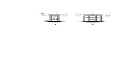
Figure 31: Contributions to the total cross section $\sigma_{tot}^{\gamma^{*}p}$: (a) the single chain representing the linear QCD evolution equations; (b) gluon production from two different gluon chains.

and they naturally explain the observed scaling behavior, $F_{2}(Q^{2},x)\approx F_{2}(Q^{2}/Q_{s}^{2}(x))$ with $Q_{s}^{2}(x)=Q_{0}^{2}(1/x)^{\lambda}$. Next, in the photoproduction region, $Q^{2}\approx 0$, direct evidence for the presence of multiple interactions also comes from the analysis of final states Gwenlan:2004iu . A further strong hint at the presence of multi-chain configurations comes from the observation of a large fraction of diffractive final states in deep inelastic scattering at HERA. In the final states analysis of the linear QCD evolution equations, it is expected that the produced partons are not likely to come with large rapidity intervals between them. In the momentum-ordered single chain picture (Fig. 31a), therefore, diffractive final states should be part of the initial conditions (inside the lower blob in Fig. 31a), i.e. they should lie below the scale $Q_{0}^{2}$ which separates the parton description from the nonperturbative strong interactions. This assignment of diffractive final states, however, cannot be

Figure 32: Hard diffractive final states.(a) dijet production; (b) the diffractive cross section as $s$-channel discontinuity of a two-ladder diagram.

complete. First, data have shown that the Pomeron which generates the rapidity gap in DIS diffraction is harder than in hadron - hadron scattering; furthermore, there are specific diffractive final states with momentum scales larger than $Q_{0}^{2}$, e.g. vector mesons built from heavy quarks and diffractive dijets (illustrated in Fig. 32): the presence of such final states naturally requires corrections to the single chain picture (Fig. 32b). From a $t$-channel point of view, both Fig. 31b and Fig. 32b belong to the same class of corrections, characterized by four gluon states in the $t$-channel.

In proton-proton collisions corrections due to multiple interactions should be important in those kinematic regions where parton densities for small momentum fractions and for not too large momentum scales are being probed, e.g. jet production near the forward direction. Another place could be the production of multijet final states (Fig. 33): multiple jets may come from different parton chains, and these contributions

Figure 33: Jet production in $pp$ collisions from two different parton chains

may very well affect the background to new physics beyond the standard model. Moreover, the modeling of multijet configurations will be necessary for understanding the underlying event structure in $pp$ collisions (see Sjostrand:2004ef and references therein).

From the point of view of collinear factorization, multiple interactions with momentum ordered parton chains are higher-twist effects, i.e they are suppressed by powers of the hard momentum scale. At small $x$, however, this suppression is compensated by powers of the large logarithms, $\ln 1/x$: multiple interactions, therefore, are mainly part of small-$x$ physics. In this kinematic region the Abramovsky-Gribov-Kanchelli (AGK)  Abramovsky:1973fm rules can be applied to the analysis of multi-gluon chains, and it is the aim of this article to present a brief overview about the current status of the AGK rules in pQCD.

As we will discuss below, in the analysis of multiple parton chains the couplings of $n$ gluons to the proton play an essential role. Regge factorization suggests that these couplings should be universal, i.e. the couplings in $\gamma^{*}p$ collisions at HERA are the same as those in $pp$ scattering at the LHC. Therefore, a thorough analysis of the role of multiple interactions in deep inelastic electron-proton scattering at HERA should be useful for a solid understanding of the structure of events at the LHC.

6.1.2 Basics of the AGK cutting rules

The original AGK paper  Abramovsky:1973fm , which was written before the advent of QCD, addresses the question how, in the optical theorem,

$$\sigma_{tot}^{pp}=\frac{1}{s}Im\,T_{2\to 2}\,\,=\,\,\sum_{f}\int d\Omega_{f}|T_{i\to f}|^{2},$$ (75)

the presence of multi-Pomeron exchanges (Fig. 34)

Figure 34: $s$-cut through a multi-Pomeron exchange: the zig-zag lines stand for nonperturbative Pomerons.

in the total hadron-hadron cross section leads to observable effects in the final states (rhs of eq.(75)). Based upon a few model-independent assumptions on the couplings of multi-Pomeron exchanges to the proton, the authors derived simple ‘cutting rules’: different contributions to the imaginary part belong to different cuts across the multi-Pomeron diagrams, and each cut has its own, quite distinct, final state characteristics. As a result, the authors found counting rules for final states with different particle multiplicities, and they proved cancellations among rescattering corrections to single-particle and double-particle inclusive cross sections.

In the QCD description of hard (or semihard) final states a close analogy appears between (color singlet) gluon ladders and the nonperturbative Pomeron: multiple parton chains (for example, the two chains in Fig. 31b) can be viewed as cuts through two perturbative BFKL Pomerons. In the same way as in the original AGK paper, the question arises how different cuts through a QCD multi-ladder diagram can be related to each other. In the following we briefly describe how AGK cutting rules can be derived in pQCD  Bartels:1996hw ; Bartels:2005wa . Subsequently we will present a few new results which come out from pQCD calculations, going beyond the original AGK rules, followed by some numerical estimates of the effects which can be expected.

One of the few assumptions made in the original AGK paper states that the coupling of the Pomerons to the external particle are (i) symmetric under the exchange of the Pomerons (Bose symmetry), and (ii) that they remain unchanged if some of the Pomerons are being cut. These properties also hold in pQCD, but they have to be reformulated: (i’) the coupling of (reggeized) gluons to external particles is symmetric under the exchange of reggeized gluons, and (ii’) it remains unchanged if we introduce cutting lines between the gluons. In QCD, however, the color degree of freedom also allows for another possibility: inside the n-gluon state (with total color zero), a subsystem of two gluons can form an antisymmetric color octet state: in this case the two gluons form a bound state of a reggeized gluon (bootstrap property). For the case of $\gamma^{*}\gamma^{*}$ scattering, explicit calculations  Bartels:1994jj have shown that the coupling of $n$ gluons to virtual photons can be written as a sum of several pieces: the fully symmetric (‘irreducible’) one which satisfies (i’) and (ii’), and other pieces which, by using the bootstrap property, can be reduced to symmetric couplings of a smaller number of gluons (‘cut reggeons’). This decomposition is illustrated in Fig. 35.

Figure 35: Decomposition of the coupling of four gluons to a virtual photon. In the last two terms on the rhs it is understood that we have to sum over different pairings of gluons at the lower end.

Since the bootstrap property is related to the reggeization of the gluon and, therefore, is expected to be valid to all orders of perturbation theory, also these properties of the couplings of multi-gluon states to external particles should be of general validity. In this short review we will mainly concentrate on the symmetric couplings.

As an illustrative example, we consider the coupling of four gluons to a proton. The simplest model of a symmetric coupling is a sum of three pieces, each of which contains only the simplest color structure:

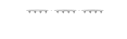
Figure 36: The symmetric coupling of four gluons to an external particle. The lines inside the blob denote the color connection, e.g. the first term has the color structure $\delta_{a_{1}a_{2}}\delta_{a_{3}a_{4}}$.

The best-known cutting rule for the four gluon exchange which follows  Bartels:1996hw ; Bartels:2005wa from this symmetry requirement is the ratio between the three different pairings of lines given in Fig. 37.

Figure 37: Different cutting lines in the four-gluon exchange.

Each term, on the partonic level, corresponds to a certain multiplicity structure of the final state: a rapidity gap (‘zero multiplicity’), double multiplicity, and single multiplicity. Simple combinatorics then leads to the ratioAbramovsky:1973fm

$$1:2:-4.$$ (76)

for the two-ladder contribution to the cross section. In order to be able to generalize and to sum over an arbitrary number of gluon chains, it is convenient to use an eikonal ansatz:

$$\begin{split}N_{2n}^{A}(\mbox{\boldmath$k$}_{1},a_{1};\ldots;&\mbox{\boldmath$k$}_{2n},a_{2n};\omega)=\\ \frac{1}{\sqrt{(N_{c}^{2}-1)^{n}}}\Biggl{(}&\sum_{Pairings}\phi^{A}(\mbox{\boldmath$k$}_{1},\mbox{\boldmath$k$}_{2};\omega_{12})\delta_{a_{1}a_{2}}\cdot\ldots\\ &\cdot\phi^{A}(\mbox{\boldmath$k$}_{2n-1},\mbox{\boldmath$k$}_{2n};\omega_{{2n-1},{2n}})\delta_{a_{2n-1}a_{2n}}\Biggr{)}\;.\end{split}$$ (77)

Inserting this ansatz into the hadron–hadron scattering amplitude, using the large-$N_{c}$ approximation, and switching to the impact parameter representation, one obtains, for the contribution of $k$ cut gluon ladders, the well-known formula:

$$ImA_{k}=4s\int d^{2}\mbox{\boldmath$b$}e^{i\mbox{\boldmath$q$}\mbox{\boldmath$b$}}P(s,\mbox{\boldmath$b$})$$ (78)

where

$$P(s,\mbox{\boldmath$b$})\;=\;\frac{[\Omega(s,\mbox{\boldmath$b$})]^{k}}{k!}e^{-\Omega(s,\mbox{\boldmath$b$})},$$ (79)

and $\Omega$ stands for the (cut) two-gluon ladder.

Another result  Bartels:2005wa which follows from the symmetry properties of the $n$ gluon-particle coupling is the cancellation of rescattering effects in single and double inclusive cross sections. In analogy with the AGK results on the rescattering of soft Pomerons, it can be shown that the sum over multi-chain contributions and rescattering corrections cancels (Fig. 38),

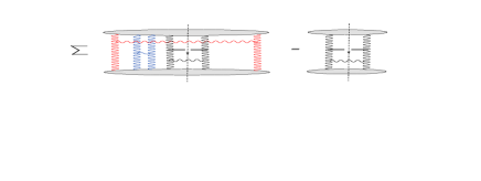
Figure 38: AGK cancellations in the one-jet inclusive cross section.

leaving only the single-chain contribution (in agreement with the factorization obtained in the collinear analysis). This statement, however, holds only for rescattering between the two projectiles: it does not affect the multiple exchanges between the tagged jet and the projectile (Fig. 39) which require a separate discussion (see below).

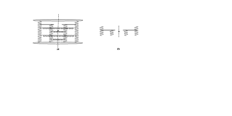
Figure 39: (a) Nonvanishing rescattering corrections in the one-jet inclusive cross section; (b) a new vertex: $g\,+\,2g\to jet$.

All these results can be generalized to include also the soft Pomeron: all one needs to assume is that the couplings of soft Pomerons and reggeized gluons are symmetric under interchanges, and they are not altered if cutting lines are introduced.

6.1.3 New results

Explicit calculations in QCD lead to further results on multiple interactions. First, in the four gluon exchange there are other configurations than those shown in Fig. 37; one example is depicted in Fig. 40. Here the pairing of gluon chains switches from $(14)(23)$ in the upper part (= left rapidity interval) to $(12)(34)$ in the lower part (= right rapidity interval).

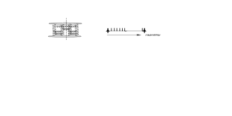
Figure 40: Decomposition into two rapidity intervals: the upper (left) interval has double multiplicity, the lower (right) one corresponds to a rapidity gap.

One can show that the ratio $1:2:-4$ holds for each rapidity interval. In  Bartels:2005wa this has been generalized to an arbitrary number of exchanged gluon lines.

Another remark applies to the applicability of the cutting rules to rescattering corrections in the single jet inclusive cross section (Fig. 39). Below the jet vertex we, again, have an exchange of four gluon lines, similar to the diagram in the middle of Fig. 37. As to the cutting rules, however, there is an important difference between the two situations. In Fig. 37, the blob above the four gluons is totally inclusive, i.e. it contains an unrestricted sum over $s$-channel intermediate states, whereas in Fig. 39 the part above the four gluon state is semi-inclusive, i.e. it contains the tagged jet. This ‘semi-inclusive’ nature destroys the symmetry above the four gluon states, and the cutting rules have to be modified  Kovchegov:2001sc ; Braun:2005ma . In particular, eqs.(77) - (78) are not applicable to the rescattering corrections between the jet and projectile. A further investigation of these questions is in progress  Bartels:2006prep .

Finally a few comments on reggeization and cut reggeons. Clearly there are more complicated configurations than those which we have discussed so far; an example appears in $\gamma^{*}p$ scattering (deep inelastic electron proton scattering). In contrast to $pp$ scattering, the coupling of multi-gluon chains to the virtual photon can be computed in pQCD, and the LO results, for the case of $n=4$ gluons, are illustrated in Fig. 41.

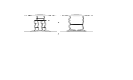
Figure 41: Four-gluon contributions to $\gamma^{*}p$ proton scattering: two equivalent ways of summing over all contributions. (a) the decomposition of Fig. 35 with the pQCD triple Pomeron vertex. (b) an alternative way of summation which explicitly shows the coupling of two Pomerons to the photon vertex and which leads to a new vertex $Z$.

It turns out that we have two alternative possibilities: in the completely inclusive case (total cross section), it is convenient to chose Fig. 41a, i.e. the sum of all contributions can be decomposed into two sets of diagrams. In the first set, at the top of the diagram two gluons couple to the quark-antiquark pair, and the subsequent transition to the four-gluon state goes via the pQCD triple Pomeron vertex. This vertex, as a function of the 4 gluons below, has the symmetry properties described above. As a result, we can apply the cutting rules to the four gluon state, as discussed before. However, there is also the second term in Fig. 41a, which consists of a two gluon state only: this is the reggeizing contribution we have mentioned before. As indicated in the figure, the splitting of the reggized gluons at the bottom amounts to a change in the (nonperturbative) coupling. We want to stress that, because of the inclusive nature of this set of diagrams, the triple Pomeron vertex $V$ in Fig. 41a, similar to the BFKL kernel, contains both real and virtual contributions. For this reason, the decomposition in Fig. 41a is applicable to inclusive cross sections, and it is not convenient for investigating specific final states such as, for example, diffractive final states with a fixed number of quarks and gluons in the final state.

There exists an alternative way of summing all contributions (Fig. 41b) which is completely equivalent to Fig. 41a but allows to keep track of diffractive $q\bar{q}$, $q\bar{q}g$,…final states: this form is illustrated in Fig. 41b. One recognizes the ‘elastic intermediate state’ which was not visible in Fig. 41a, and the new triple Pomeron vertex $Z$ which contains only real gluon production. This vertex $Z$, as discussed in Bartels:2004hb is no longer symmetric under permutations of the gluons at the lower end; consequently, we cannot apply the AGK cutting rules to the four gluon states below. These findings for multiple scattering effects in DIS imply, strictly speaking, that cross sections for diffractive $q\bar{q}$ or $q\bar{q}g$ states cannot directly be inserted into the counting rules (76).

Also $pp$ scattering will contain corrections due to multiple interactions which are more complex. There are, for example, graphs which contain the $2\to 4$ gluon vertex $V$, leading to a change of the number of gluon lines (Fig. 42).

Figure 42: A correction in which the number of lines changes. The black vertex denotes the $2\to 4$ gluon vertex.

Since this $2\to 4$ gluon vertex, as a function of the four gluons below the vertex, satisfies the symmetry requirements listed above, we can apply our previous analysis to the cutting lines below the vertex. In addition, however, one can ask how the lines continue above the $2\to 4$ gluon vertex: we show two examples, one of them containing a cut (reggeized) gluon. Concentrating on this two-gluon state (i.e. we imagine that we have already summed over all possible cutting lines below the vertex $V$), the counting rules are quite different: in contrast to the even-signature Pomeron, the gluon is a odd-signature reggeon. Consequently, the cut gluon is suppressed w.r.t. the uncut gluon by one power in $\alpha_{s}$, and this suppression leads to the following hierarchy of cutting lines: the cut between the gluons belongs to leading order, the cut through one of the two reggeized gluons is suppressed by one power in $\alpha_{s}$, the cut through both reggeized gluons is double suppressed (order $\alpha_{s}^{2}$). A closer analysis of this question is under investigation Bartels:2006prep .

6.1.4 Conclusions

Corrections due to multiple interactions seem to be important in DIS at small $x$ and low $Q^{2}$; they are expected to play a significant role also in multijet production in $pp$ scattering. The study of the AGK rules to pQCD provides help in understanding the systematics of multiple gluon chains. Results described in this review represent the beginning of a systematic analysis. We have listed a few questions which require further work.

As an immediate application, we believe that a quantitative analysis of multiple scattering at HERA will provide a useful input to the modeling of final states at the LHC.

6.2 Experimental consequences

Main author H. Kowalski

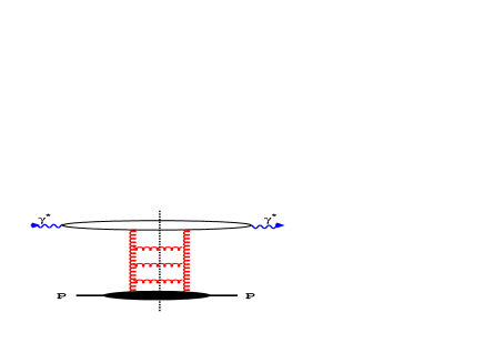
Figure 43: The single gluon-ladder contribution to the total $\gamma^{*}p$ cross section. The blob at the lower end of the diagrams contains the physics below the scale $Q_{0}^{2}$ which separates hard from soft physics, whereas the blob at the upper end contains hard physics that can be described by pQCD. The dashed line denotes the cut.

Experimentally it is easy to differentiate between diffractive and single or multiple inclusive final states since diffractive states exhibit large rapidity gaps. The multiple inclusive final states should also be distinct from the single inclusive ones since, at least naively, we would expect that in the multiple case the particle multiplicity should be considerably higher. At low $x$, however, the relation between the number of virtual states excited in the interaction (as measured by $F_{2}$) and the final particle multiplicity cannot be straightforward since the growth of $F_{2}$ with decreasing $x$ is faster than the multiplicity increase. This may indicate that the hadronization mechanism may be different from the string picture commonly used in the hadronization procedure of single chain parton showers. The influence of multiple scattering on the particle multiplicity of the final states should also be damped by the energy conservation. The cut through several Pomerons leads clearly to more gluons produced in the final state, but the available energy to produce particles in the hadronization phase remains the same. A detailed Monte Carlo program is therefore necessary to evaluate this effect.

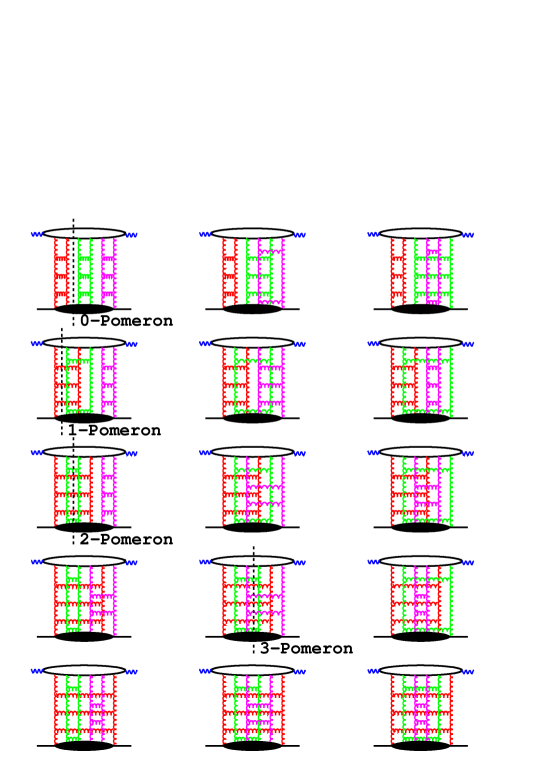
Figure 44: 3-Pomeron contributions to the elastic $\gamma^{*}p$ amplitude. All 15 possible diagrams are shown with some examples of Pomeron cuts.

The number of diagrams contributing to the reaction amplitude increases very quickly with the number of Pomerons. For the 3-Pomeron amplitude the gluons can be paired in 15 possible ways, shown in Fig. 44 with the examples of 0-Pomeron, 1-Pomeron, 2-Pomeron and 3-Pomeron cuts. For $m$-Pomerons the number of possible gluon pairs and also diagrams is:

$$(2m-1)(2m-3)(2m-5)....=(2m-1)!/(2^{m-1}(m-1)!).$$

Assuming that all the diagrams for a given multi-Pomeron exchange amplitude contribute in the same way, the above analysis suggests that the probability for different cuts to contribute should be given by the combinatorial factors. This is the content of the AGK rules which were obtained from the analysis of field theoretical diagrams well before QCD was established Abramovsky:1973fm and which relate the cross-section, $\sigma_{k}$, for observing a final state with $k$-cut Pomerons with the amplitudes for exchange of $m$ Pomerons, $F^{(m)}$:

$$\sigma_{k}=\sum_{m=k}^{\infty}(-1)^{m-k}\,2^{m}\,\frac{m!}{k!(m-k)!}F^{(m)}.$$ (80)

The same result is also obtained from a detailed analysis of the Feynman diagram contributions in QCD above with the oversimplified assumption that only the symmetric part of the two-gluon couplings contributes Bartels:2005wa .

6.3 Multiple Interactions in the Dipole Model

Main author H. Kowalski

The properties of the multi-Pomeron amplitude and of the cut Pomeron cross-sections can be quantitatively studied in a dipole model. Along the lines which were discussed in section 5 the $\gamma^{*}p$ interaction proceeds in three stages: first the incoming virtual photon fluctuates into a quark-antiquark pair, then the $q\bar{q}$ pair elastically scatters on the proton, and finally the $q\bar{q}$ pair recombines to form a virtual photon. The total cross-section for $\gamma^{*}p$ scattering, or equivalently $F_{2}$, is obtained by averaging the dipole cross-sections with the photon wave functions, $\psi(r,z)$, and integrating over the impact parameter, $b$:

$$F_{2}=\frac{Q^{2}}{4\pi^{2}\alpha_{em}}\int d^{2}r\int\frac{dz}{4\pi}\psi^{*}\psi\int d^{2}b\frac{d\sigma_{qq}}{d^{2}b}.$$ (81)

Here $\psi^{*}\psi$ denotes the probability for a virtual photon to fluctuate into a $q\bar{q}$ pair, summed over all flavors and helicity states. The dipole cross-section is assumed to be a function of the opacity $\Omega$:

$$\frac{d\sigma_{qq}}{d^{2}b}=2\,\left(1-\exp(-\frac{\Omega}{2})\right).$$ (82)

At small-$x$ the opacity $\Omega$ can be directly related to the gluon density, $xg(x,\mu^{2})$, and the transverse profile of the proton, $T(b)$:

$$\Omega=\frac{\pi^{2}}{N_{C}}\,r^{2}\,\alpha_{s}(\mu^{2})\,xg(x,\mu^{2})\,T(b).$$ (83)

The parameters of the gluon density are determined from the fit to the total inclusive DIS cross-section Kowalski:2003hm . The transverse profile was determined from the exclusive diffractive $J/\Psi$ cross-sections Kowalski:2003hm . The opacity function $\Omega$ determined in this way has predictive properties; it allows to describe other measured reactions, e.g. charm structure function or elastic diffractive $J/\Psi$ production.

For a small value of $\Omega$ the dipole cross-section, eg. (82), is equal to $\Omega$ and therefore proportional to the gluon density. This allows to identify the opacity with the single Pomeron exchange amplitude of Fig. 43. The multi-Pomeron amplitude is determined from the expansion:

$$\begin{split}\frac{d\sigma_{qq}}{d^{2}b}=&2\,\left(1-\exp(-\frac{\Omega}{2})\right)\\ =&2\,\sum_{m=1}^{\infty}(-1)^{m-1}\,\left(\frac{\Omega}{2}\right)^{m}\frac{1}{m!}\end{split}$$ (84)

as

$$F^{(m)}=\left(\frac{\Omega}{2}\right)^{m}\frac{1}{m!},$$ (85)

since the dipole cross-section can be expressed as a sum of multi-Pomeron amplitudes Mueller:1996te in the following way:

$$\frac{d\sigma_{qq}}{d^{2}b}=2\,\sum_{m=1}^{\infty}(-1)^{m-1}\,F^{(m)}.$$ (86)

The cross-section for k  cut Pomerons is then obtained from the AGK rules, eq. (80), and from the multi-Pomeron amplitude, eq. (85), as:

$$\begin{split}\frac{d\sigma_{k}}{d^{2}b}=&\sum_{m=k}^{\infty}(-1)^{m-k}\,2^{m}\,\frac{m!}{k!(m-k)!}\left(\frac{\Omega}{2}\right)^{m}\frac{1}{m!}\\ =&\frac{\Omega^{k}}{k!}\sum_{m=k}^{\infty}(-1)^{m-k}\,\frac{\Omega^{m-k}}{(m-k)!}\end{split}$$ (87)

which leads to a simple expression:

$$\frac{d\sigma_{k}}{d^{2}b}=\frac{\Omega^{k}}{k!}\exp(-\Omega).$$ (88)

The diffractive cross-section is given by the difference between the total and the sum over all cut cross-sections:

$$\begin{split}\frac{d\sigma_{diff}}{d^{2}b}=&\frac{d\sigma_{tot}}{d^{2}b}-\sum_{k=1}^{\infty}\frac{d\sigma_{k}}{d^{2}b}\\ =&2\left(1-\exp\left(-\frac{\Omega}{2}\right)\right)-(1-\exp(-\Omega))\\ =&\left(1-\exp\left(-\frac{\Omega}{2}\right)\right)^{2}\end{split}$$ (89)

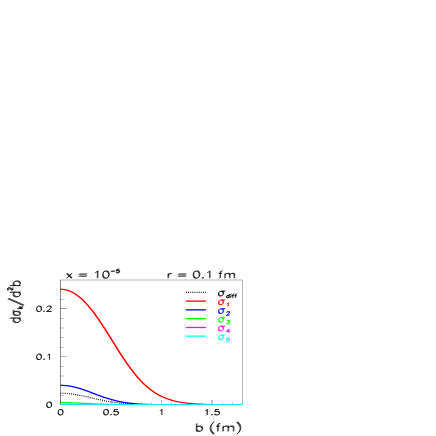
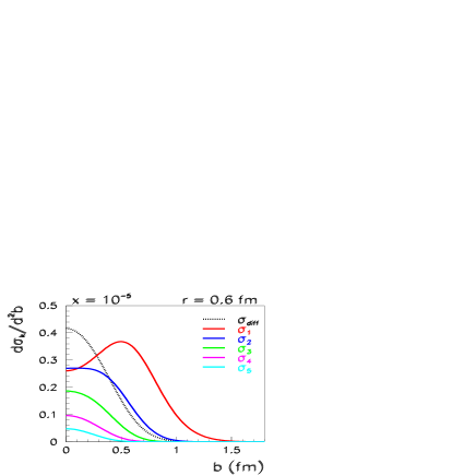
Figure 45: Examples of $b$ dependence of various cut dipole and diffractive cross-sections.

The cut cross-sections determined in the dipole model analysis of HERA data have several interesting properties shown in Fig. 45: for small dipoles ($r=0.1$ fm) the opacity $\Omega$ is also small, so the single cut cross-section, $\sigma_{1}$, dominates. This leads to particle production emerging only from the one-cut pomeron, which should correspond, in the context of e.g. the LUND model, to a fragmentation of only one string. For larger dipoles ($r=0.6$ fm) the dipole cross-section starts to be damped in the middle of the proton (at $b\approx 0$) by saturation effects. Therefore, the single cut cross-section is suppressed in the middle while the multiple cut cross-sections, $\sigma_{2},\;\sigma_{3}$, etc, become substantial and increasingly concentrated in the proton center. These, fairly straightforward properties of dipoles indicate that in the central scattering events the multiple scattering probability will be enhanced, which may lead at the LHC to substantial effects in a surrounding event multiplicity.

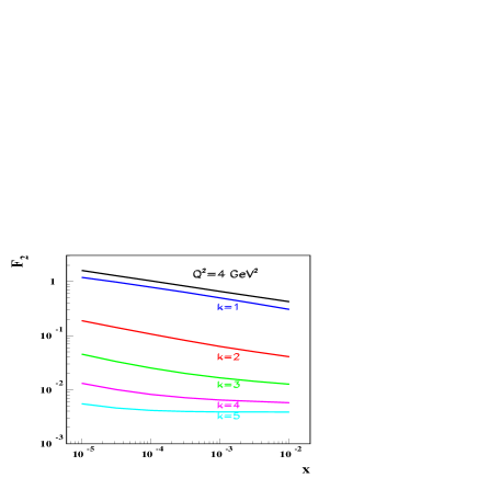
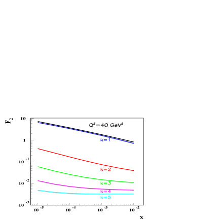
Figure 46: $F_{2}$ and the contributions of k-cut Pomeron processes, $F_{2}^{k}$.

The contribution to $F_{2}$ from the $k$-cut Pomeron exchanges are computed in the analogous way to $F_{2}$:

$$F_{2}^{k}=\frac{Q^{2}}{4\pi^{2}\alpha_{em}}\int d^{2}r\int\frac{dz}{4\pi}\psi^{*}\psi\int d^{2}b\frac{d\sigma_{k}}{d^{2}b}.$$ (90)

These contributions are shown, together with $F_{2}$, as a function of $x$ for two representative $Q^{2}$ values in Fig. 46. One finds that multiple interaction contributions, i.e. $k\geq 2$, in the perturbative region, at $Q^{2}=4$ GeV², are substantial. In the typical HERA range of $x\approx 10^{-3}-10^{-4}$, the $k=2$ contribution is around 10% of $F_{2}$ and the contributions of higher cuts are also non-negligible. For example, the contribution of the 5-cut Pomeron exchanges is still around 0.5%, which means that at HERA, many thousand events may come from this type of process.

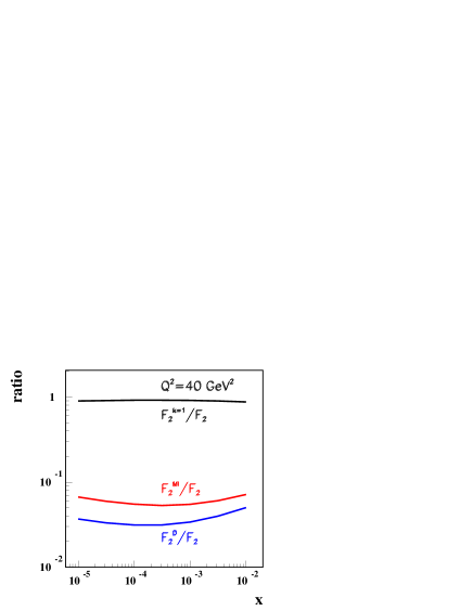
Figure 47: Fractions of single (k=1), multiple interaction (MI) and diffraction (D) in DIS.

Figure 47 shows the fraction of the multiple interaction processes, $F_{2}^{MI}=F_{2}^{k=2}+F_{2}^{k=3}+F_{2}^{k=4}+F_{2}^{k=5}$ in $F_{2}$, at the same $Q^{2}$ values. At $Q^{2}=4$ GeV² the fraction of multiple scattering events is around 14% and at $Q^{2}=40$ GeV² around 6%, in the HERA $x$ region, which indicates that the decrease of multiple scattering with increasing $Q^{2}$ is only logarithmic. The fraction of diffractive processes, shown for comparison, is of the same order, and drops also logarithmically with $Q^{2}$. The logarithmic drop of the diffractive contribution expected in the dipole model is confirmed by the data Chekanov:2005vv .

The dipole model provides a straightforward extrapolation to the region of low $Q^{2}$, which is partly perturbative and partly non-perturbative. Figure 48 shows the contribution to $F_{2}$ of $k$-cut Pomeron processes and the fractions of multiple interactions and diffractive processes at $Q^{2}=0.4$ GeV².

Note also that, as a byproduct of this investigation, the ratio of diffractive and inclusive cross-sections, $F^{D}_{2}/F_{2}$ is found to be almost independent of $x$, in agreement with the data and also other dipole model predictions Chekanov:2005vv ; Golec-Biernat:1999qd ; Bartels:2002cj . The absolute amount of diffractive effects is underestimated, since the evaluation of diffraction through AGK rules is oversimplified. It is well known Bartels:2002cj , that a proper evaluation of diffraction should also take into account the $q\bar{q}g$ contribution which is missing in the simple AGK schema.

Hence, we find that the impact parameter dependent dipole saturation model Kowalski:2003hm reproduces well the main properties of the data and leads to the prediction that multiple interaction effects at HERA should be of the order of diffractive effects, which are known to be substantial. The multiple interaction effects should decrease slowly (logarithmically) with increasing $Q^{2}$, similarly to the diffractive contribution.

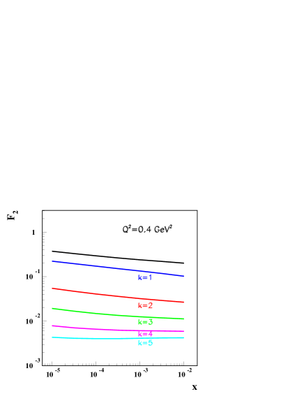
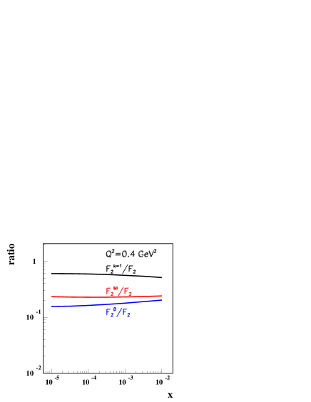
Figure 48: Left: $F_{2}$ and the contributions of $k$-cut Pomeron processes. Right: Fractions of single (k=1), multiple interaction (MI) and diffraction (D) in DIS at $Q^{2}=0.4$ GeV².

7 Experimental comparisons

With the luminosity collected at HERA during the past years very precise measurements of the proton structure function, $F_{2}(x,Q^{2})$, have been performed over a large range in the fractional proton energy, $x$, and in the photon virtuality, $Q^{2}$. The measurements are now limited by systematic errors rather than statistical. Parton density functions have been obtained mainly by fitting the DGLAP equations, evolved from an input scale $Q_{0}^{2}$, to the structure functions, measured at some scale $Q^{2}$. Especially the precision data at low $Q^{2}$ have provided an important input to various QCD fit analyses. It was recognized early that inclusive measurements, like that of structure functions, are not very sensitive to the new parton dynamics expected to appear in the low $x$ region. Instead evidence from such dynamics has to be found from investigations of hadronic final states in a phase space region where the DGLAP governed evolution is suppressed. Thus, a global fit, which also includes data from more exclusive processes, would further constrain the PDFs. A problem is that measurements of the hadronic final states suffer from much larger uncertainties than the inclusive structure function measurements and therefore measurements of many different complementary processes are desirable.

Forward jet production in DIS is expected to be sensitive to new dynamics and early results indeed showed a deviation from the predictions of the LO DGLAP model as well as of NLO calculations. However, with the inclusion of resolved photon contributions, DGLAP provided the same level of agreement as the colour diple model (CDM), in which the parton emission follows the same scheme as in the new dynamics proposed. Only recent studies of final states with a ’forward jet and two additional jets’ give the first evidence for parton dynamics in which there is additional breaking of the $k_{t}$-ordering compared to that predicted by the resolved photon model.

Dijet data may be used to gain better insight into the dynamics of the parton evolution and for extracting updf’s. In the low $x$ region boson-gluon fusion processes are dominating and in the LO DGLAP description the gluon and the photon collide head on in the hadronic center-of-mass system and thus will be produced back-to-back. Deviations from this may arise from additional radiation and if the parton propagator, entering the hard scattering process, has significant transverse momentum, such that the two partons produced in the hard intreraction are no longer balanced in transverse momentum. Thus, the two jets produced will not be back-to-back in azimuth. A measurement of the azimuthal correlation between the two jets should be directly sensitive to the predictions of models based on different evolution schemes.

The flavour composition of the final state can also provide important information about the evolution and production mechanisms of partons. This has motivated a measurement of final states with identified strange particles.

Although $F_{2}$ data can be well described by the exchange of a single gluon ladder, it is unlikely that a single chain generates large rapidity gaps, which is the signature of diffractive processes. The traditional picture of diffractive processes is scattering by the virtual photon against a pomeron with a partonic structure. Over the past years significant progress in the understanding of diffraction has been made at HERA, which has led to a modification of this description. Data are much better described assuming multi-gluon exchange, where a pair of gluons is the minimum to create a colour singlet state. The multi-pomeron exchange model provides a natural connection between inclusive scattering, diffractive scattering and multiple scattering given by different cuts through the ladder diagrams according to the so called AGK cutting rules, as discussed in section 6. Rapidity gaps between high-transverse energy jets have been observed at the Tevatron, at a fraction that is in good agreement with BFKL predictions. Also multiple scattering has been studied at the Tevatron, and found to give significant contributions to the final state. In $ep$-collisions at HERA multiple interactions can occur in processes where the exchanged photon interacts via its parton content. Through the possibility to control the fraction of the photon momentum, $x_{\gamma}$, entering into the scattering process, more systematic investigations of underlying events may be performed at HERA over a wide energy range.

In general, measurements of final states provide information about the hard scattering process, parton evolution, initial and final state radiation and multiple interactions. Thus, it is important to measure, as accurately as possible, the final states in order to test the theoretical models.

In the following the studies of multiple interactions, gaps between jets, forward jets and strange particle production will be discussed in more detail.

7.1 Multiple interactions at the Tevatron and HERA

Main author J. Turnau

Since hadrons are composite objects of quarks and gluons there is a certain probability that collisions between hadrons involve more than one parton interaction i.e. we have multiple interactions (MI). As a consequence of the strong rise of the parton distribution at low $x$ the probability to have MI increases with the collision energy and the effect at the Tevatron has turned out to be significant. At the LHC the contribution from MI will be even larger. In electron-proton collisions at HERA MI may occur in processes where the exchanged photon is resolved and interacts via its parton content. The final state of collisions with MI will thus contain the products of the primary hard collisions, those of additional soft or semihard parton interactions, contributions from initial and final state radiation and from the beam remnants. All products not coming from the primary interaction contribute to the so called underlying event (UE).

Effects of MI will influence the total cross section, the inclusive jet cross section, the jet multiplicity, the jet profile, the jet pedestal (the level of transverse energy outside the jets), the transverse energy flow and transverse energy correlations, the hadron multiplicity, the multiplicity correlations and may cause large multiplicity fluctuations. Experimental data from HERA and the Tevatron have been compared to various theoretical models containing a description of MI.

7.1.1 Monte Carlo models for description of multiple interactions

So far multiple interactions are theoretically not well understood. The theoretical description is mainly based on QCD inspired models, which assume a hard scattering process superimposed on soft or semi-hard interactions. Various models differ in how initial and final state radiation is taken into account as well as how the hadronization process and the beam remnants are treated.

HERWIG Marchesini:1991ch ; Corcella:2000bw assumes that the UE is a soft collision between the two beam “clusters”. The parameters of this model are tuned to describe experimental results on soft hadron-hadron collisions. Also the strength and frequency parameters of the secondary interactions are subject to tuning. There is a possibility to include multiparton interactions by employing an interface to the JIMMY generator Butterworth:1996zw ; HERALHC:Jimmy . To some extent the formalism that is used to describe MI in JIMMY is the same as in PYTHIA (see below).

PYTHIA Sjostrand:2000wi assumes that each interacting beam hadron (or resolved photon) leaves behind a beam remnant, which does not radiate. In contrast to the original HERWIG and ISAJET generators PYTHIA uses multiple parton interactions to enhance the activity of the UE. In the simplest version of the PYTHIA multiple interaction model, the transverse momentum cut-off of the hard interactions is lowered to $p_{t}^{mia}<p_{t}^{min}$. The mean number of (semi-) hard interactions is given by $<n>=\sigma_{parton}(p_{t}^{mia})/\sigma_{nd}$, where $\sigma_{nd}$ is the non-diffractive part of the total cross section. The distribution of the number of interactions is not uniquely determined. In the simplest approach the fluctuations are calculated from a Poisson distribution. In the more sophisticated version the number of interactions are given by a Poisson distribution for each given impact parameter, where the impact parameter dependence is given by a double-Gaussian overlap function. The number of additional interactions is typically of order 1 -2 . The parton process with the highest transverse momentum in the partonic final state can be calculated by the quark/gluon $2\to 2$ matrix element. Additional parton interactions in the event are calculated from perturbative gluon-gluon scattering processes.

Simulations of photon-hadron processes have frequently been performed using the PHOJET generatorEngel:1994vs . PHOJET was designed to simulate, in a consistent way, all components which contribute to the total photoproduction cross section. In contrast to PYTHIA, PHOJET incorporates both multiple soft- and (semi-)hard parton interactions on the basis of a dual unitarization scheme Capella:1986cm .

In their initial investigations of UE Affolder:2001xt CDF used the ISAJET Monte Carlo Paige:2003mg , which does not include multiple scattering a la PYTHIA or HERWIG. Instead the beam jets are added assuming that they are identical to a minimum bias event at the energy remaining after the hard scattering. However, ISAJET did not describe the UE data and has not been used in subsequent analyses.

Generally speaking, the Monte Carlo models which include multiple scattering have enough free parameters to describe the most important features of data from HERA, the Tevatron and of other data found in the JetWeb database Butterworth:2002ts . A program to tune the model parameters is under way.

7.1.2 Underlying events at the Tevatron

In the standard analysis of hard scattering events one measures jet cross sections and jet properties, which in general are very well described by QCD Monte Carlo models and NLO QCD calculations, provided that jet pedestals are properly parameterized. The uncertainty in the UE contribution to jet events is actually dominating the systematic errors for inclusive jet measurements. In order to understand the physics of UE, special studies which go far beyond a simple parameterization of the energy flow outside the jets, are required.

The CDF collaboration at the Tevatron has performed Affolder:2001xt ; Acosta:2004wq detailed studies of the structure and properties of the underlying event in two complementary analyses of Run I data at $\sqrt{(}s)=1800$ and $\sqrt{(}s)=630$   GeV. The overall event structure was investigated using global variables such as charged particle multiplicities and the scalar sum of the transverse momenta of charged particles as a function of the leading jet momentum. The sensitivity to UE is expected to be the highest in phase space regions perpendicular to the direction of the leading jet. In the first analysis Affolder:2001xt jets were defined by applying the simple cone algorithm to charged particles only. Since the lower limit of the jet transverse momenta (scalar $p_{T}$ sum) was chosen as low as 0.5  GeV, UE could be studied in the transition region from minimum bias events to events with high transverse momentum jets. In a later analysis Acosta:2004wq jets were defined using the cone algorithm on calorimetric objects with $E_{T}>15-20\,\mbox{GeV}$.

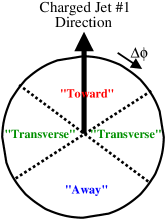
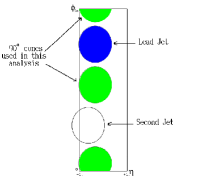
Figure 49: LEFT: Illustration of correlations in the azimuthal angle $\Delta\phi$ relative to the direction of leading charged jet in the event. The regions $\mid{\Delta\phi}\mid<60$, $\mid\Delta\phi\mid>120$ and $60<\mid{\Delta\phi}\mid<120$ are referred to as “towards”, “away” and “transverse”. Each region covers the same range $\mid\Delta\eta\mid\times\mid\Delta\phi\mid=2\times 120^{\circ}$. On an event by event basis the regions “transverse minimum/maximum” are defined to be the ones containing the minimum/maximum transverse momentum.
RIGHT: The phase space regions, as defined in the analysis Affolder:2001xt , shown in the $\eta-\phi$ plane, where the “transverse” regions are given by cones at $\pm 90^{\circ}$ to the leading jet direction.

As shown in Fig. 49 (left) the direction of the leading jet in each event is used to define different regions in $\eta-\phi$ space : “toward”, “away” and “transverse”. The “transverse” region is particularly sensitive to the UE. In ref.  Acosta:2004wq the “transverse” region was defined as the area in the $\eta-\phi$ plane covered by the two cones with radii $R=\sqrt{(\Delta\eta)^{2}+(\Delta\phi)^{2}}=0.7$ perpendicular to the highest energy jet (Fig. 49 right). On an event-by-event basis the regions of “minimal” and “maximal” transverse momentum were defined as the regions containing the smallest and largest scalar $p_{T}$ sum of charged particles, respectively. Such an investigation of the UE helps separating the initial and final state radiation component from the “beam remnant” components. It can be argued that transverse energy in the “minimal transverse” region ($P_{T}^{90,min}$) is due to multiple scattering while the difference in transverse momentum between the “minimal-” and “maximal transverse” regions $\Delta P_{T}^{90}=P_{T}^{90,max}$-$P_{T}^{90,min}$ is a measure of the hard initial/final state radiation connected to the primary interaction. The CDF analyses have established several basic properties of UE, illustrated in Figs 50 (from Affolder:2001xt ) and 51 (from Acosta:2004wq ) and listed below.

• In the “transverse” regions most sensitive to UE, the average number of charged particles and the average charged scalar $p_{T}$ sum grow very rapidly with the momentum of the leading jet. At $p_{T}(jet)>5~{}\,\mbox{GeV}$ an approximately constant plateau is observed (Fig.  50). The height of this plateau is at least twice that observed in ordinary soft collisions at the corresponding energy. Although models including multiple scatterings (soft or semi-hard) predict a growth of both the average number of charged particles and the average charged scalar $p_{T}$ sum at low momenta of the leading jet, they are not able to describe the data in this region ($p_{T}(jet)<5~{}\,\mbox{GeV}$).

• For the leading jet above 50 GeV, $P_{T}^{90,min}$ is almost independent on the momentum of the leading jet which is correctly described by HERWIG and PYTHIA.

• The difference $\Delta P_{T}^{90}$ increases slowly.

• Neither PYTHIA nor HERWIG are able to reproduce the $P_{T}$ distribution of tracks in minimum bias events (not shown).

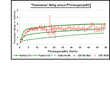
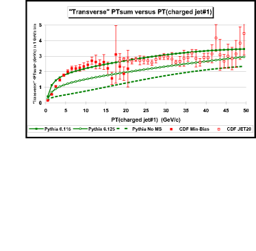
Figure 50: Data (taken from Affolder:2001xt ) on the average number of charged particles ($p_{T}>0.5\,\mbox{GeV},\mid\eta\mid<1$) (top) and the scalar $p_{T}$ sum of charged particles (bottom) in transverse region defined in Fig. 49 as a function of transverse momentum of the leading charged jet compared with Monte Carlo Models.

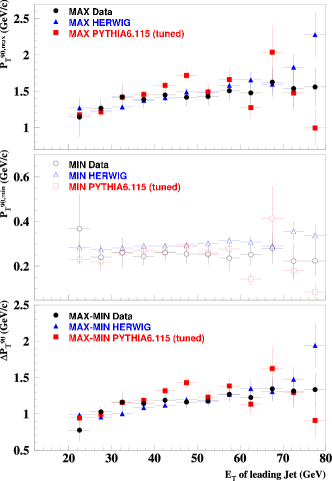
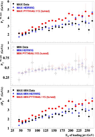
Figure 51: $P_{T}^{90,max},P_{T}^{90,min}$ and $\Delta P_{T}^{90}$ as a function of $E_{T}$ of the highest energy jet at $\sqrt{s}=1800~{}\,\mbox{GeV}$ (bottom three plots) and $\sqrt{s}=630~{}\,\mbox{GeV}$ (top three - plots) taken from Acosta:2004wq . PYTHIA has been tuned to describe the data.

In summary, the QCD models implemented in the PYTHIA and HERWIG Monte Carlo programs are able to describe the most important features of the UE from the Tevatron data. In both cases the agreement is reached only after careful tuning of many parameters, in particular the regularization scale of the transverse momentum. Clearly the experimental tests of the predictions from PYTHIA and HERWIG concerning correlations and fluctuations in the UE will be an important challenge over the coming yearsHERALHCButtar .

7.1.3 Underlying event energy at HERA

At HERA, the interaction of electrons and protons via the exchange of a quasi-real photon can result in the production of jets. The photon may interact as a point-like particle in so called direct process (Fig. 52a) or it may interact via its partonic structure such that a parton carrying a fraction $x_{\gamma}$ of the photon momentum interacts with a parton in the proton.

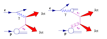
Figure 52: Examples of LO QCD diagrams for photoproduction of inclusive jets in direct (a) and resolved (b) photon interactions.

In resolved processes the photon remnant can interact with the proton remnant very much like in hadron hadron collisions. The center of mass energy in the $\gamma p$ system extends up to 300  GeV, much below the reach of the Tevatron. Thus the effects of MI at HERA are certainly weaker and more difficult to study. On the other hand studies of the photon properties from measurements of UE at HERA are interesting and complementary to the measurements at hadron-hadron colliders. The experimental results presented in this section have been published by the H1 collaboration Aid:1995ma . They are based on a sample where photoproduction events are tagged by detecting the scattered electron and it contains 3 sub-samples : the minimum bias sample (charged track with momentum$>0.3$  GeV+ reconstructed vertex), the high- $E_{T}$ sample (total transverse energy in the pseudorapidity range $-0.8<\eta<3.3$; $E_{T}>20$ GeV) and the jet sample ( at least 1 jet with $E_{T}>7$ GeV).

At HERA the amount of energy which is carried by the photon remnant can be estimated using the variable

$$x_{\gamma}^{jets}=\frac{E_{T}^{jet1}e^{-\eta^{jet1}}+E_{T}^{jet2}e^{-\eta^{jet2}}}{2E_{\gamma}}$$

where $x_{\gamma}^{jets}$ is the fraction of the photon energy carried by interacting parton, $E_{T}^{jet1}$ and $E_{T}^{jet2}$ are the energies of the two jets with the highest transverse energies, and $\eta^{jet1}$ and $\eta^{jet2}$ are their pseudorapidities. The energy of the photon, $E_{\gamma}$, is determined from the energy measured in the electron tagger. Fig. 53(a) from ref. Aid:1995ma shows the transverse energy density outside the jets of 2-jet events in the central rapidity region. The data decrease as $x_{\gamma}^{jets}\rightarrow 1$ to the level measured in deep inelastic $ep$ scattering events, dominated by direct photon processes. The dashed line in Fig. 53 indicates the energy density measured in minimum bias events (for which $x_{\gamma}^{jets}$ is not measurable). At small $x_{\gamma}^{jets}$ the energy density increases to the level found in hadron-hadron collisions ($\approx 0.3$ at the SPS and the Tevatron). Both PHOJET and PYTHIA with the MI parameters suitably tuned ($p_{t}^{mia}$ depending on choice of the the photon pdf) are able to reproduce the data. This type of the measurement apparently has no analog in hadron-hadron collisions.

Figure 53: a: The transverse energy density outside jets in the central rapidity region, $\mid\eta_{\gamma p}\mid<1$, of $\gamma p$ collisions as a function of the momentum fraction $x_{\gamma}^{jet}$ of the parton entering the hard scattering process from the photon side. The data (taken from Aid:1995ma ) are compared to models with multiple interactions (PYTHIA mia, PHOJET) and without (PYTHIA). The dashed horizontal line marks the energy density level of minimum bias events.
b: the observed rapidity correlations with respect to the central rapidity of $\gamma p$ collisions, $\eta^{\star}=0$. The dashed (dotted) histogram represents calculations of the QCD generator PYTHIA with (without) interactions of the beam remnants.

Energy-energy correlations are sensitive measures of how the energy is distributed over the available phase space and provide important information for the modeling of UE. The rapidity correlation $\Omega$ is defined as

$$\begin{split}&\Omega(\eta^{*})\\ &=\frac{1}{N_{ev}}\sum_{i=1}^{N_{e}v}\frac{(\langle E_{T,\eta^{*}=0}\rangle-E_{T,\eta^{*}=0})_{i}(\langle E_{T,\eta^{*}}\rangle-E_{T,\eta^{*}})_{i}}{(E_{T}^{2})_{i}}\end{split}$$ (91)

Here $E_{T}$ is the total transverse energy measured in the H1 calorimeter and the other terms refer to transverse energies measured in pseudorapidity bins of size $\Delta\eta=0.22$ in the $\gamma p$ cms. The average values were extracted from all events in the sample. Fig. 53 (b) shows the rapidity correlations from the high $E_{T}$ sample. The data show a short range correlation around the reference bin $\eta^{*}=0$ and a long range anti-correlation which results from the hard scattering process. PYTHIA without MI predicts an anti-correlation which is too strong. Adding MI i.e. the addition of uncorrelated energy to the event results in a correct description of the data. The same conclusion holds for an event sample where jets are explicitly required (jet sample).

In summary, the underlying event in photoproduction events can be consistently interpreted as the superposition of a hard scattering process and interactions between the beam spectators, as modeled by PYTHIA and PHOJET. Processes with resolved photons at $x_{\gamma}\approx 0$ are found to produce 3.5 times the transverse energy density of minimum bias events comparable with that observed in hadron-hadron collisions at the SPS (UA1) and the Tevatron (CDF). Studies of energy-energy correlations demonstrate that the additional transverse energy in the event is not correlated with the hard scattering process. Finally, the contribution of higher order radiation to UE can be studied separately using the kinematic quantity $x_{\gamma}$ to switch off the beam remnant interactions.

7.1.4 Explicit Observations of Double Hard Scattering

The general signature of multiple parton scattering is an increase in the transverse energy flow of the event. However, in extreme cases, the transverse energy of a secondary interaction is sufficient to produce an additional pair of jets. The observation of such events is highly important for several reasons. It is sensitive to the phenomenology of multiple parton interactions and provides direct information on the structure of the proton in transverse space. It is also important for estimating backgrounds to processes producing di-boson ($W^{+}W^{-}$, etc.) and boson + jets at the LHC.

Double parton scattering (DP) in the simplest model produces a final state that mimics a combination of two independent scatterings. It is customary Abe:1993rv to express the cross section for this process as a product of the cross sections for the individual hard scatterings divided by a scaling factor, $\sigma_{eff}$:

$$\sigma_{DP}=m\frac{\sigma_{A}\sigma_{B}}{2\sigma_{eff}}.$$

The factor $m$ is unity for indistinguishable scatterings and has a value of two when it is possible to distinguish between A and B. This formula assumes that the number of parton-parton interactions follows a Poisson distribution but can also use other distributions e.g. Poisson statistics for a given impact parameter Calucci:1997uw . The parameter $\sigma_{eff}$ describes the spatial distribution of partons Sjostrand:1987su e.g. for a model that assumes a proton with uniformly distributed partons $\sigma_{eff}=11$ mb.

Events with four or more high transverse momentum objects (jets, leptons, prompt photons…) is an obvious place to look for signatures of multiple hard parton interactions, although it should be realized that higher order QCD processes, for which no exact QCD calculations are available yet, are dominating. Only few searches for double parton collisions at the ISR, the SPS and the Tevatron have been performed and the results are not very consistent Akesson:1986iv ; Alitti:1991rd ; Abe:1993rv . Recently CDF published Abe:1997xk a strong signal for double parton scattering. In this analysis a value of $\sigma_{eff}=14.5\pm 1.7^{+1.7}_{-2.3}$ mb was extracted from data in a model-independent way by comparing the number of observed double parton events to the number of events with hard scatterings at the separate $p\bar{p}$ collisions within the same beam crossing. This represents a significant improvement over previous measurements and may be used to constrain models using a parton spatial density.

7.1.5 Multiple interaction component of the underlying event at Tevatron and HERA : summary

Analyses of hadron-hadron and photon-hadron collisions at the Tevatron and HERA have firmly established the multiple interaction component of the underlying event. Only QCD models which include secondary soft or semi-hard scatterings a la Sjostrand:1987su (PYTHIA, HERWIG, PHOJET) are able to give a reasonable description of the data. The energy flow of underlying events as measured outside leading jets was studied in various phase space regions, applying conditions which help to disentangle contributions from beam-beam interaction and initial/final state radiation. At HERA the energy available to the photon beam remnant was used as an additional constraint. The general structure of the underlying event is reasonably well described by Monte Carlo generators like PYTHIA, HERWIG and PHOJET, but a detailed understanding is still missing. Studies of underlying events at HERA are not as extensive as those by CDF at the Tevatron and it would certainly be of great interest to apply the same analysis methods to high energy $\gamma p$, where $x_{\gamma}$ provides an additional “degree of freedom”. The effects of the transverse size of hadronic photon on the underlying event, i.e. the $Q^{2}$ dependence, has not been exploited at all so far. The CDF Collaboration has reported a firm observation of double hard parton scattering in the $\gamma$ + 3 jets final state and has made an estimation of the effective cross section for double parton scattering. This fact is of paramount importance for the phenomenological understanding of the underlying event, in constraining the multiple interaction models Sjostrand:1987su ; Odagiri:2004tt .

7.2 Gaps between jets and BFKL

Main author G. Ingelman

The observation Abe:1997ie ; Abbott:1998jb at the Tevatron of events with a rapidity gap between two high transverse-energy ($E_{T}$) jets provides strong evidence for BFKL dynamics in terms of color singlet gluon ladder exchange Enberg:2001ev . As illustrated in Fig. 54, the process can be described by elastic parton-parton scattering via a hard color singlet gluon ladder. Since there is no color exchanged, no color fields (strings) will be formed in between and hence no hadrons produced through hadronization in the intermediate rapidity region.

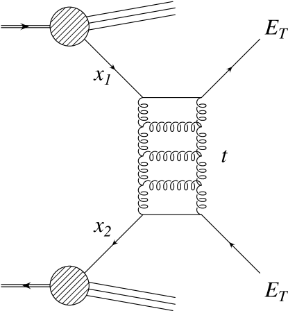
Figure 54: Hard color singlet exchange through a BFKL gluon ladder giving a rapidity gap between two high-$p_{\perp}$ jets.

In the high energy limit $s/|t|\gg 1$, where the parton cms energy is much larger than the momentum transfer, the amplitude for this diagram is dominated by terms $\sim[\alpha_{s}\,\ln(s/|t|)]^{n}$ where the smallness of $\alpha_{s}$ is compensated by the large logarithm. These terms are resummed in the BFKL equation, which describes the exchange of the whole gluon ladder, including virtual corrections and reggeization of gluons. When solving the equation numerically it was found that non-leading corrections are very important at the non-asymptotic energy of the Tevatron Enberg:2001ev ; Motyka:2001zh .

Formulating the results as matrix elements for effective $2\to 2$ parton scattering processes, they could be implemented in the Lund Monte Carlo Pythia such that parton showers and hadronization could be added to generate complete events. As shown in Fig. 55 these reproduce the data, both in shape and absolute normalization, which is not at all trivial. The non-leading corrections are needed since the asymptotic Mueller-Tang result has the wrong $E_{T}$ dependence. A free gap survival probability parameter, which in other models is introduced to get the correct overall normalization, is not needed in this approach. Amazingly, the correct gap rate results from the complete model including parton showers, parton multiple scattering and hadronization through Pythia together with the soft color interaction model Edin:1995gi ; Edin:1996mw . The latter accounts for QCD rescatterings Brodsky:2004hi that are always present and if these are ignored one needs to introduce an ad hoc 15% gap survival probability factor.

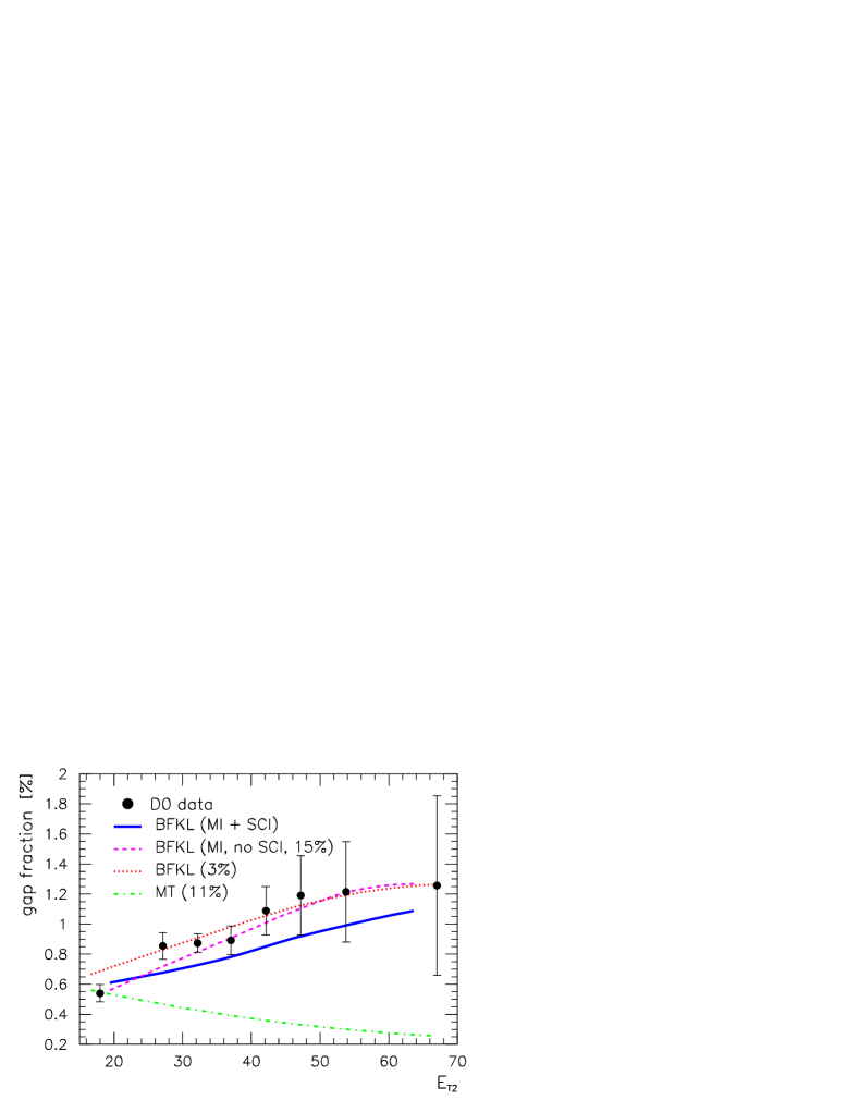
Figure 55: Fraction of jet events having a rapidity gap in $|\eta|<1$ between the jets versus the second-highest jet-$E_{T}$. D0 data compared to the color singlet exchange mechanism Enberg:2001ev based on the BFKL equation with non-leading corrections and with the underlying event treated in three ways: simple 3% gap survival probability, Pythia’s multiple interactions (MI) and hadronization requiring a 15% gap survival probability, MI plus soft color interactions (SCI) and hadronization with no need for an overall renormalization factor. Also shown is the Mueller-Tang (MT) asymptotic result with a 11% gap survival probability.

Related to this is the new results from ZEUS ZEUS-diffr-psi-t on the production of $J/\psi$ at large momentum transfer $t$ in photoproduction at HERA. The data, shown in Fig. 56, agree well with perturbative QCD calculations Enberg:2002zy , based on the hard scales $t$ and $m_{c\bar{c}}$, for two-gluon BFKL color singlet exchange. As illustrated in Fig. 57, not only the simple two-gluon exchange is included, but also the full gluon ladder in either leading logarithm approximation or with non-leading corrections. Using a running $\alpha_{s}$ does, however, give a somewhat too steep $t$-dependence compared to the data. The conventional DGLAP approximation provides a good description in the range $|t|<m^{2}_{J/\psi}$ where this model Gotsman:2001ne is argued to be valid due to ordered momenta in the gluon ladder (cf. Fig. 57). However, the DGLAP model gives a very weak dependence on the energy $W$, which is in contrast to the observed increase of the cross-section with energy as also results from the BFKL-based calculations ZEUS-diffr-psi-t . Altogether this provides another evidence for BFKL dynamics.

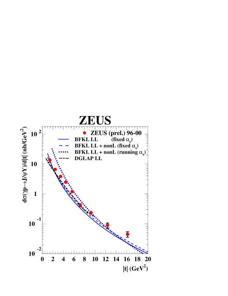
Figure 56: Differential cross-section $d\sigma/d|t|$ for the process $\gamma+p\to J/\psi+Y$. ZEUS data compared ZEUS-diffr-psi-t to BFKL model calculations using leading log (LL) with fixed $\alpha_{s}$, and including non-leading (non-L) corrections with fixed or running $\alpha_{s}$ as well as with a model based on leading log DGLAP.

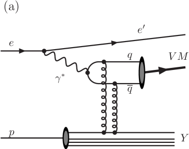
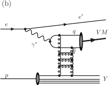
Figure 57: Diffractive vector meson production at large momentum transfer as described by perturbative QCD hard color singlet exchange via two gluons and a gluon ladder in the BFKL framework Enberg:2002zy .

7.3 Jets at small-$x$

Main authors L. Jönsson and A. Knutsson

In the region of low $x$-values the interacting parton frequently produces a cascade of emissions before it interacts with the virtual photon. Due to the strong ordering in virtuality, the emissions of the DGLAP evolution are very soft close to the proton direction, whereas BFKL emissions can produce large transverse momenta in this region. Thus, deviations from the DGLAP parton evolution scheme are expected to be most visible in a region close to the direction of the proton beam.

HERA has extended the available region in the Bjorken scaling variable, $x_{Bj}$, down to values of $x_{Bj}\simeq 10^{-4}$, for values of the four momentum transfer squared, $Q^{2}$, larger than a few GeV², where perturbative calculations in QCD are expected to be valid.

A measurement of the forward jet production cross section at small $x_{Bj}$, as proposed by Mueller and Navelet Mueller:1990er ; Mueller:1990gy ; Mueller:1986ey , has long been regarded as the most promising test of perturbative parton dynamics. The idea is to select events with a jet close to the proton direction having the virtuality of the propagator closest to the proton approximately equal to the virtuality of the exchanged photon. This will suppress an evolution with strong ordering in virtuality as is the case in the DGLAP evolution. The additional requirement that the forward jet takes a large fraction of the proton momentum, $x_{jet}=E_{jet}/E_{p}$, such that $x_{jet}\gg x_{Bj}$ opens up for an evolution where the propagators are strongly ordered in the longitudinal momentum fraction like in the BFKL scheme. Experimentally this is realized by demanding the squared transverse momentum of the forward jet to be of the same order as $Q^{2}$ and $x_{jet}$ to be larger than a preselected value which still gives reasonable statistics. More exclusive final states, like those containing a di-jet system in addition to the forward jet (called ‘2+forward jet’), provide an additional handle to control the parton dynamics.

Production of forward jets in DIS

The H1 experiment has measured the forward jet cross section Aktas:2005up using data collected in 1997, comprising an integrated luminosity of 13.7 pb^-1. The proton energy is 820 GeV and the positron energy is 27.6 GeV which correspond to a center-of-mass-energy of $\sqrt{s}\approx$300 GeV.

DIS events are obtained by applying the cuts $E_{e^{\prime}}>10$ GeV, $156^{\circ}<\theta_{e}<175^{\circ}$, $0.1<y<0.7$ and $5$ GeV${}^{2}<Q^{2}<85$ GeV², where $E^{\prime}_{e}$ is the energy of the scattered electron, $\theta_{e}$ the polar angle, and $y$ is the inelasticity of the exchanged photon. Jets are defined using the inclusive $k_{t}$-jet algorithm Catani:1993hr ; Catani:1992zp applied in the Breit-frame. A forward jet is defined in the laboratory system as having $p_{t,jet}>3.5$ GeV and being in the angular range $7^{\circ}<\theta_{jet}<20^{\circ}$. In order to enhance BFKL evolution it is required that $x_{jet}>0.035$ whereas DGLAP evolution was suppressed in the single differential cross section measurement by introducing the requirement $0.5<p_{t}^{2}/Q^{2}<5$.

Another event sample, called the ’2+forward jet’ sample, is selected by requiring that, in addition to the forward jet, at least two more jets are found, all of them having $p_{t,jet}$ larger than 6 GeV. In this scenario the $p_{t}^{2}/Q^{2}$-cut is not applied, due to the limited statistics.

The forward jet cross sections for single and triple differential cross sections are compared to LO ($\alpha_{s}$) and NLO ($\alpha_{s}^{2}$) calculations of direct photon interactions as obtained from the DISENT program. Comparisons of the inclusive forward jet cross sections with the DISENT predictions for a di-jet final state are adequate, since the forward jet events always contain at least one additional jet due to the kinematics. The renormalization scale $(\mu_{r}^{2})$ is given by the average $p_{t}^{2}$ of the di-jets from the hard scattering process, while the factorization scale $(\mu_{f}^{2})$ is given by the average $p_{t}^{2}$ of all forward jets in the selected sample.

In the analysis of events with two jets in addition to the forward jet, the measured cross sections are compared to the predictions of NLOJET++. This program provides perturbative calculations of cross sections for three-jet production in DIS at NLO ($\alpha^{3}_{s}$) accuracy. In this case the scales $\mu_{r}=\mu_{f}$ are set to the average $p_{t}^{2}$ of the three selected jets in the calculated event.

The NLO calculations by DISENT Catani:1996jh ; Catani:1996vz and NLOJET++ Nagy:2001xb are performed using the CTEQ6M Pumplin:2002vw parameterization of the parton distributions in the proton.

Single Differential Cross Section

The measured single differential forward jet cross sections on hadron level are compared with LO ($\alpha_{s}$) and NLO ($\alpha^{2}_{s}$) calculations from DISENT in Fig. 58a. In Fig. 58b and c the data are compared to the various QCD models.

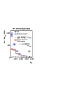
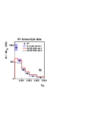
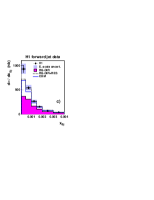
Figure 58: The hadron level cross section for forward jet production as a function of $x_{Bj}$ as measured by H1 Aktas:2005up compared to NLO predictions from DISENT (a) and to QCD Monte Carlo models (b and c). The shaded band around the data points shows the error from the uncertainties in the energy scales of the liquid argon calorimeter and the SpaCal electromagnetic calorimeter. The hatched band around the NLO calculations illustrates the theoretical uncertainties in the calculations, estimated as described in the text. The dashed line in (a) shows the LO contribution.

In Fig. 58a it can be observed that, at small $x_{Bj}$, the NLO di-jet calculations from DISENT are significantly larger than the LO contribution. This reflects the fact that the contribution from forward jets in the LO scenario is suppressed by kinematics. For small $x_{Bj}$ the NLO contribution is an order of magnitude larger than the LO contribution. The NLO contribution opens up the phase space for forward jets and improves the description of the data considerably. However, the NLO di-jet predictions are still a factor of 2 below the data at low $x_{Bj}$. The somewhat improved agreement at higher $x_{Bj}$ can be understood from the fact that the range in the longitudinal momentum fraction which is available for higher order emissions decreases.

From Fig. 58b it is seen that the CCFM model (both set-1 and set-2) predicts a somewhat harder $x_{Bj}$ distribution, which results in a comparatively poor description of the data.

Fig. 58c shows that the DGLAP model with direct photon interactions alone (RG-DIR) gives results similar to the NLO di-jet calculations and falls below the data, particularly in the low $x_{Bj}$ region. The description of the data by the DGLAP model is significantly improved if contributions from resolved virtual photon interactions are included (RG-DIR+RES). However, there is still a discrepancy in the lowest $x_{Bj}$-bin, where a possible BFKL signal would be expected to show up most prominently. The CDM model, which gives emissions that are non-ordered in transverse momentum, shows a behavior similar to the RG DIR+RES model.

Events with Reconstructed Di-jets in Addition to the Forward Jet

By requiring the reconstruction of the two hardest jets in the event in addition to the forward jet, different kinematic regions can be investigated by applying cuts on the jet momenta and their rapidity separation.

In this scenario it is demanded that all jets have transverse momenta larger than 6 GeV. By applying the same $p_{t,jet}$ cut to all three jets, evolution with strong $k_{t}$-ordering is not favored. The jets are ordered in rapidity according to $\eta_{fwdjet}>\eta_{jet_{2}}>\eta_{jet_{1}}>\eta_{e}$ with $\eta_{e}$ being the rapidity of the scattered electron. The cross section is measured by H1 Aktas:2005up in two intervals of $\Delta\eta_{1}=\eta_{jet_{2}}-\eta_{jet_{1}}$. If the di-jet system originates from the quarks $q_{1}$ and $q_{2}$ (see Fig. 59), the phase space for evolution in $x$ between the di-jet system and the forward jet is increased by requiring that $\Delta\eta_{1}$ is small and that $\Delta\eta_{2}=\eta_{fwdjet}-\eta_{jet_{2}}$ is large. $\Delta\eta_{1}<1$ favors small invariant masses of the di-jet system and thereby small values of $x_{g}$ (see Fig. 59). With $\Delta\eta_{2}$ large, $x_{g}$ carries only a small fraction of the total propagating momentum, leaving the rest for additional radiation.

The directions of the other jets are related to the forward jet through the $\Delta\eta$ requirements. When $\Delta\eta_{2}$ is small, it is therefore possible that one or both of the additional jets originate from gluon radiation close in rapidity space to the forward jet. With $\Delta\eta_{1}$ large, BFKL-like evolution may then occur between the two jets from the di-jet system, or, with both $\Delta\eta_{1}$ and $\Delta\eta_{2}$ small, even between the di-jet system and the hard scattering vertex. By studying the cross section for different $\Delta\eta$ values one can test theory and models for event topologies where the $k_{\perp}$ ordering is broken at varying locations along the evolution chain.

Figure 59: A schematic diagram of an event giving a forward jet and two additional hard jets. These may stem from the quarks ($q_{1}$ and $q_{2}$) in the hard scattering vertex or gluons in the parton ladder. $x_{g}$ is the longitudinal momentum fraction carried by the gluon, connecting to the hard di-jet system (in this case $q_{1}$ and $q_{2}$) .

In this investigation the same settings of the QCD models are used as in sections 7.3, while the NLO three-jet cross sections are calculated using NLOJET++.

From Fig. 60 it is observed that NLO three-jet gives good agreement with the data if the two additional hard jets are emitted in the central region ($\Delta\eta_{2}$ large). It is interesting to note that a fixed order calculation ($\alpha_{s}^{3}$), including the $\log(1/x)$-term to the first order in $\alpha_{s}$, is able to describe these data well. However, the more the additional hard jets are shifted to the forward region ($\Delta\eta_{2}$ small), the less well are the data described by NLO three-jet. A possible explanation is that the more forward the additional jets go, the higher the probability is that one of them, or even both, do not actually originate from quarks but from additional radiated gluons. NLO three-jet calculates the NLO contribution to final states containing one forward jet and two jets from the di-quarks, i.e. it accounts for the emission of one gluon in addition to the three jets. Since the radiated gluon is predominantly soft it has a small probability to produce a jet that fulfills the transverse momentum requirement applied in this analysis. This results in a depletion of the theoretical cross section in the small $\Delta\eta_{2}$ region, which is more pronounced when $\Delta\eta_{1}$ is also small, i.e. when all three jets are in the forward region. Consequently a significant deviation between data and NLOJET++ can be observed for such events (see the lowest bin in Fig. 60b). Accounting for still higher orders in $\alpha_{s}$ might improve the description of the data in this domain, since an increased number of gluon emissions would enhance the probability that one of the radiated gluons produces a jet which is above the threshold on the transverse momentum.

As explained above, evolution with strong $k_{\perp}$-ordering is disfavored in this study. Radiation that is non-ordered in $k_{\perp}$ may occur at different locations along the evolution chain, depending on the values of $\Delta\eta_{1}$ and $\Delta\eta_{2}$. In a comparsion to QCD models (these figures are not shown, for details see Aktas:2005up ) the following observations where made. The colour dipole model gives good agreement in all cases, whereas the LO DGLAP models give cross sections that are too low except when both $\Delta\eta_{1}$ and $\Delta\eta_{2}$ are large. For this last topology all models and the NLO calculation agree with the data, indicating that the available phase space is exhausted and that little freedom is left for dynamical variations.

Furthermore it was seen that the ‘2+forward jet’ sample differentiates between the CDM and the DGLAP-resolved model, in contrast to the more inclusive samples where CDM and RG-DIR+RES give the same predictions. The conclusion is that additional breaking of the $k_{\perp}$ ordering is needed compared to what is included in the resolved photon model (see Ref. Aktas:2005up ).

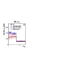
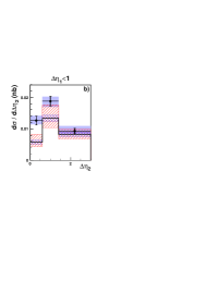
Figure 60: The cross section for events with a reconstructed high transverse momentum di-jet system and a forward jet as a function of the rapidity separation between the forward jet and the most forward-going additional jet, $\Delta\eta_{2}$ as measured by H1 Aktas:2005up . Results are shown for the full sample and for two ranges of the separation between the two additional jets, $\Delta\eta_{1}<1$ and $\Delta\eta_{1}>1$. The data are compared to the predictions of a three-jet NLO calculation from NLOJET++. The band around the data points illustrates the error due to the uncertainties in the calorimetric energy scales. The band around the NLO calculations illustrates the theoretical uncertainties in the calculations.

7.4 Production of neutral strange particles in deep-inelastic scattering at HERA

Main author C. Risler

In deep-inelastic scattering strange particles can be produced either if a strange quark is interacting in the hard subprocess, or if strange quark pairs are produced during the hadronization process. The production of strange particles is sensitive to soft and hard parton radiation of the initial and final state partons and is thus a complementary approach to small $x$ processes. Other sources of strangeness can be the decays of charm hadrons or more exotic particles like glueballs, pentaquarks or instantons.

The production properties of strange particles are not yet fully understood nor described by the QCD models. Since strange particles are also produced during the hadronization process, a measurement of strange particle production is also a means to test the universality of hadronization in $e^{+}e^{-}$, $pp$ or $ep$ collisions.

The inclusive production cross sections of strange neutral particles, namely $K^{0}_{S}$-mesons and $\Lambda$-baryons, in deep-inelastic $ep$-scattering at HERA were measured with the H1 detector Risler:2003np . The analyzed data were collected in the years 1996 and 1997 at a center of mass energy of 300 GeV and with an integrated luminosity of 17.8 ${\rm pb}^{-1}$. The kinematic region $2\,{\rm GeV}^{2}<Q^{2}<100\,{\rm GeV}^{2}$ and $0.1<y<0.6$ is investigated, where $Q^{2}$ is the squared momentum transfer and y the inelasticity. This allows for probing very low Bjorken-$x$, $x>10^{-5}$. $K^{0}_{S}$ mesons and $\Lambda$ baryons are reconstructed via the decay to $\pi^{-}\pi^{+}$ and $\pi^{-}p$, respectively. The production of $K^{0}_{S}$ and $\Lambda$ is measured within the visual range, defined by $-1.3<\eta<1.3$ and $0.5\,{\rm GeV}<p_{T}<3.5\,{\rm GeV}$, where $\eta$ is the pseudorapidity and $p_{T}$ the transverse momentum in the laboratory frame.

Comparisons of the total $K^{0}_{S}$ and $\Lambda$ cross sections with models using the Lund string hadronization Artru:1974hr ; Bowler:1981sb ; Andersson:1983ia ; Andersson:1983jt ; Andersson:1985qr show that a lower strangeness suppression factor of $\lambda_{s}\approx 0.2-0.25$ is preferred to the default value of $\lambda_{s}=0.3$.

The differential cross sections in the laboratory and the Breit frame are compared to different model predictions, namely the MEPS (matrix element and parton shower) model using the RAPGAP event generator Jung:1995gf , CCFM Ciafaloni:1988ur ; Catani:1990yc ; Catani:1990sg implemented in the CASCADE program Jung:2000hk ; Jung:2001hx , the color dipole model (CDM) Gustafson:1988rq ; Andersson:1990dp ; Gustafson:1992uh ; Andersson:1989gp ; Gustafson:1986db ; Lonnblad:1992tz using DJANGOH Charchula:1994kf and to predictions by the HERWIG Marchesini:1991ch ; Corcella:2000bw event generator. The HERWIG prediction for the $\Lambda$ cross section is normalized to the observed total cross section, since HERWIG overestimates the cross section by a factor of 3.

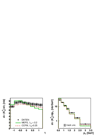
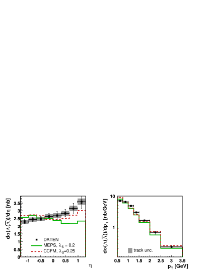
Figure 61: Differential $K^{0}_{S}$ and $\Lambda$ production cross sections in the laboratory frame.

Fig. 61 shows the $\eta$ and $p_{T}$ dependence of the $K^{0}_{S}$ and $\Lambda$ cross sections in the laboratory frame compared to the model predictions by MEPS and CCFM, using a strangeness suppression factor of $\lambda_{S}=0.2$ and $\lambda_{S}=0.25$ in the Lund string model, respectively. The preliminary data are shown with statistical and systematic errors; the systematic uncertainty of the cross section due to the uncertainty of the tracking efficiency is separately shown as a grey band.
The $\eta$ spectrum of $K^{0}_{S}$ production can not be reproduced by the MEPS model, while CCFM gives a better description. In $\Lambda$ production a rise in the forward direction, defined by the direction of the outgoing proton beam, is observed, which is not present in any of the models. The $p_{T}$ distribution of the $K^{0}_{S}$ and the $\Lambda$ cross section are too soft in MEPS as well as in CCFM.

The CCFM model yields a better description of the $\eta$ spectra in the data than the MEPS model. In addition, CCFM, in its implementation in the CASCADE program, allows only for gluon induced hard subprocesses.

In Fig. 62 the data are compared to a modified MEPS model (BGF), where only boson gluon fusion processes are taken into account, while quark induced subprocesses are switched off. This modified MEPS model gives a slightly better description of the data than the standard MEPS predictions.

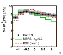
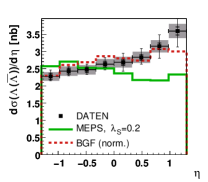
Figure 62: $\eta$ dependence of $K^{0}_{S}$ and $\Lambda$ cross sections in the laboratory frame compared to MEPS and a modified MEPS model with only BGF hard subprocess.

The differential $K^{0}_{S}$ and $\Lambda$ production cross sections are investigated as functions of $x_{p}=2|\vec{p}|/Q$ and $p_{T}$ in the Breit frame.

The Breit frame can be divided into the target hemisphere of the fragmenting proton and the current hemisphere in the direction of the incoming photon, which is related to the fragmentation of the current quark.

In the target hemisphere of the Breit frame (fig. 63) all four models underestimate the $K^{0}_{S}$ and $\Lambda$ cross section at large $x_{p}$ and the $p_{T}$ spectra are modeled too softly in most of the models.

Only a small fraction of all $K^{0}_{S}$ and $\Lambda$ decays is found in the current hemisphere of the Breit frame, leading to large statistical errors of the differential cross sections shown in Fig. 64. Within these errors CDM gives the best description of the $x_{p}$ and $p_{T}$ dependence of the differential $K^{0}_{S}$ and $\Lambda$ cross sections.

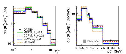
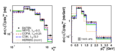
Figure 63: Target hemisphere of the Breit frame: $x_{p}=2|\vec{p}|/Q$ and $p_{T}$ dependence of $K^{0}_{S}$ and $\Lambda$ cross sections in the target hemisphere of the Breit frame.

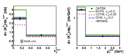
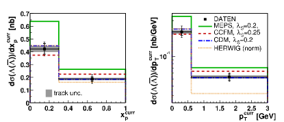
Figure 64: Current hemisphere of the Breit frame: $x_{p}=2|\vec{p}|/Q$ and $p_{T}$ dependence of $K^{0}_{S}$ and $\Lambda$ cross sections in the current hemisphere of the Breit frame.

Concluding one can say that none of the models gives a satisfactory description of the observed cross sections of neutral strange particle production. In particular the simulated transverse momentum spectra are too soft. A significant increase of $\Lambda$-baryon production was observed in the region $0<\eta<1.3$ in the laboratory frame, which is not reproduced by any of the models.

The comparison with QCD models using the Lund string hadronization reveals that a lower strangeness suppression factor than the standard LEP-value seems to be preferred at HERA.

The cross sections and comparisons shown here are results of a PhD thesis Risler:2003np .

8 Outlook

Studies of QCD in high energy $ep$ collisions are interesting in themselves, as a highly nontrivial theory due to its nonlinear nature with a nontrivial vaccuum. It is also important in order to fully understand the background in attempts to find signals for physics beyond the standard model at the LHC and future high energy colliders.

For the timelike cascades in $e^{+}e^{-}$-annihilation, experimental data are reproduced to an extent beyond expectations, by a perturbative parton cascade (if only the first gluon emission is adjusted to matrix elements) followed by a model for the subsequent non-perturbative hadronization. To describe the spacelike cascades in $ep$ scattering at high energies poses a much more difficult challenge. $k_{\perp}$-factorization and leading order BFKL evolution offer a qualitative frame of reference at small $x$, but do not give a quantitative description of the experimental data. Non-leading contributions are large, and the separation between perturbative and non-perturbative effects in the timelike cascades is not realised in the corresponding spacelike processes.

The non-leading contributions are essential also for the behaviour at asymptotic energies. They give asymptotically small corrections to the evolution equation, but not to its solution. The leading order equation fixes the solution to the powerlike form $\sim x^{-\lambda}$ (with logarithmic corrections), but the power $\lambda$ is affected by the non-leading terms, which therefore have a very large effect. The perturbative–non-perturbative interplay is important in two regimes. Firstly, the random walk in $\ln k_{\perp}^{2}$, characteristic for the BFKL evolution chain, extends down into the soft regime. This problem is further enhanced by a running coupling $\alpha_{s}$. Secondly, the high gluon densities at small $x$ imply that unitarity constraints and saturation become essential. This means that non-perturbative effects are important also at larger $k_{\perp}$, where the running coupling is small.

Recent progress, described in this report, includes in particular:

• Extending the $k_{\perp}$-factorization formalism introducing two-scale unintegrated and doubly unintegrated PDFs and investigation of the importance of the correct kinematics even at lowest order.

• The solution to the BFKL evolution at NLO, and the NLO $\gamma^{*}$ impact factor.

• BFKL dynamics in other fields, exemplified by $Q\bar{Q}$-production and away-from-jet energy flow in $e^{+}e^{-}$-annihilation.

• Studies of unitarity corrections and saturation via the Balitsky-Kovchegov equation.

• Going beyond leading order in the BK equation, where in particular energy-momentum conservation has a large effect.

• AGK cutting rules in QCD, multi-pomeron exchange and diffraction.

• Phenomenological applications and comparisons with experimental data. Here studies of forward jet and heavy quark production are of particular interest.

Further work is still needed within all these fields. The impact parameter dependence and correlations, as well as generalisations to $eA$ collisions, need to be studied. This is particularly important to get a better understanding of high energy proton-proton collisions. To fully understand the dynamics of small-$x$ physics we need in the future also to be able to combine the different routes listed above in a unifying formalism, which can simultaneously account for the effects of NLO (and NNLO) contributions and unitarity and saturation effects including multi-pomeron exchange, pomeron loops and diffraction.

The detailed understanding of small-$x$ physics is essential for the understanding of the underlying event structure observed at Tevatron and which is expected to be even more significant at the LHC. Small $x$ physics is an important issue on its own right and is important also for the understanding of the QCD background for any searches. Small $x$ physics is very complicated due to the large phase space opened but it offers also the possibility to understand the transition from a dilute to a dense system in a systematic way and thus contributes much to the understanding of complicated processes in general.

References

- (1) V. N. Gribov, L. N. Lipatov, Sov. J. Nucl. Phys. 15 (1972) 438.
- (2) L. N. Lipatov, Sov. J. Nucl. Phys. 20 (1975) 94.
- (3) G. Altarelli, G. Parisi, Nucl. Phys. B126 (1977) 298.
- (4) Y. L. Dokshitzer, Sov. Phys. JETP 46 (1977) 641.
- (5) S. Moch, J. A. M. Vermaseren, A. Vogt, Nucl. Phys. Proc. Suppl. 135 (2004) 137.
- (6) E. A. Kuraev, L. N. Lipatov, V. S. Fadin, Sov. Phys. JETP 44 (1976) 443.
- (7) E. A. Kuraev, L. N. Lipatov, V. S. Fadin, Sov. Phys. JETP 45 (1977) 199.
- (8) I. I. Balitsky, L. N. Lipatov, Sov. J. Nucl. Phys. 28 (1978) 822.
- (9) L. V. Gribov, E. M. Levin, M. G. Ryskin, Phys. Rept. 100 (1983) 1.
- (10) E. M. Levin, M. G. Ryskin, Y. M. Shabelski, A. G. Shuvaev, Sov. J. Nucl. Phys. 53 (1991) 657.
- (11) S. Catani, M. Ciafaloni, F. Hautmann, Nucl. Phys. B366 (1991) 135.
- (12) J. C. Collins, R. K. Ellis, Nucl. Phys. B360 (1991) 3.
- (13) V. S. Fadin, L. N. Lipatov, Phys. Lett. B429 (1998) 127.
- (14) M. Ciafaloni, G. Camici, Phys. Lett. B430 (1998) 349.
- (15) M. Ciafaloni, D. Colferai, G. P. Salam, Phys. Rev. D60 (1999) 114036.
- (16) G. P. Salam, Acta Phys. Polon. B30 (1999) 3679.
- (17) J. Kwiecinski, A. D. Martin, P. J. Sutton, Z. Phys. C71 (1996) 585.
- (18) L. H. Orr, W. J. Stirling, Phys. Rev. D56 (1997) 5875.
- (19) H. Kharraziha, L. Lönnblad, JHEP 03 (1998) 006.
- (20) H. Jung, Comput. Phys. Commun. 143 (2002) 100.
- (21) J. R. Andersen, W. J. Stirling, JHEP 02 (2003) 018.
- (22) B. Andersson et al., Eur. Phys. J. C25 (2002) 77.
- (23) J. R. Andersen et al., Eur. Phys. J. C35 (2004) 67.
- (24) M. Ciafaloni, Nucl. Phys. B296 (1988) 49.
- (25) S. Catani, F. Fiorani, G. Marchesini, Phys. Lett. B234 (1990) 339.
- (26) S. Catani, F. Fiorani, G. Marchesini, Nucl. Phys. B336 (1990) 18.
- (27) G. Marchesini, Nucl. Phys. B445 (1995) 49.
- (28) M. G. Ryskin, A. G. Shuvaev, Y. M. Shabelski, Phys. Atom. Nucl. 64 (2001) 1995.
- (29) H. Jung, Un-integrated uPDFs in CCFM, 2004, hep-ph/0411287.
- (30) S. Aid et al., Nucl. Phys. B470 (1996) 3.
- (31) C. Adloff et al., Eur. Phys. J. C21 (2001) 33.
- (32) M. Derrick et al., Z. Phys. C72 (1996) 399.
- (33) S. Chekanov et al., Eur. Phys. J. C21 (2001) 443.
- (34) D. A. e. a. CDF Coll., Phys. Rev. D 71 (2005) 092001.
- (35) V. M. Abazov et al., Phys. Rev. Lett. 94 (2005) 221801.
- (36) B. Abbott et al., Phys. Lett. B487 (2000) 264.
- (37) F. Abe et al., Phys. Rev. D53 (1996) 1051.
- (38) F. Abe et al., Phys. Rev. D55 (1997) 2546.
- (39) D. Acosta et al., Phys. Rev. D69 (2004) 072004.
- (40) S. Chekanov et al., Nucl. Phys. B729 (2005) 492.
- (41) G. Flucke, AIP Conf. Proc. 792 (2005) 815.
- (42) A. Szczurek, N. N. Nikolaev, W. Schafer, J. Speth, Phys. Lett. B500 (2001) 254.
- (43) A. Aktas et al., Eur. Phys. J. C33 (2004) 477.
- (44) M. Luszczak, A. Szczurek, Phys. Lett. B594 (2004) 291.
- (45) M. Hansson, H. Jung, Status of CCFM: Un-integrated gluon densities, 2003, hep-ph/0309009.
- (46) G. Watt, A. D. Martin, M. G. Ryskin, Eur. Phys. J. C31 (2003) 73.
- (47) G. Watt, A. D. Martin, M. G. Ryskin, Phys. Rev. D70 (2004) 014012.
- (48) J. C. Collins, X. Zu, JHEP 03 (2005) 059.
- (49) J. C. Collins, D. E. Soper, G. Sterman, Nucl. Phys. B250 (1985) 199.
- (50) H. Jung, G. P. Salam, Eur. Phys. J. C19 (2001) 351.
- (51) M. A. Kimber, A. D. Martin, M. G. Ryskin, Phys. Rev. D63 (2001) 114027.
- (52) J. Kwiecinski, A. D. Martin, A. M. Stasto, Phys. Rev. D56 (1997) 3991.
- (53) C. Adloff et al., Phys. Lett. B542 (2002) 193.
- (54) A. Gawron, J. Kwiecinski, Phys. Rev. D70 (2004) 014003.
- (55) J. Kwiecinski, A. Szczurek, Nucl. Phys. B680 (2004) 164.
- (56) B. Abbott et al., Phys. Lett. B513 (2001) 292.
- (57) C. Balazs et al., A comparison of predictions for SM Higgs boson production at the LHC, 2004, hep-ph/0403052.
- (58) G. Bozzi, S. Catani, D. de Florian, M. Grazzini, Phys. Lett. B564 (2003) 65.
- (59) H. Jung, Mod. Phys. Lett. A19 (2004) 1.
- (60) A. V. Lipatov, N. P. Zotov, Eur. Phys. J. C44 (2005) 559.
- (61) M. Luszczak, A. Szczurek, Unintegrated gluon distributions and Higgs boson production in proton proton collisions, 2005, hep-ph/0504119.
- (62) G. Corcella, S. Moretti, Phys. Lett. B590 (2004) 249.
- (63) G. Corcella, M. H. Seymour, Nucl. Phys. B565 (2000) 227.
- (64) A. D. Martin, R. G. Roberts, W. J. Stirling, R. S. Thorne, Phys. Lett. B531 (2002) 216.
- (65) D. A. Ross, Phys. Lett. B431 (1998) 161.
- (66) G. P. Salam, JHEP 07 (1998) 019.
- (67) M. Ciafaloni, D. Colferai, G. P. Salam, A. M. Stasto, Phys. Lett. B587 (2004) 87.
- (68) M. Ciafaloni, D. Colferai, G. P. Salam, A. M. Stasto, Phys. Rev. D68 (2003) 114003.
- (69) M. Ciafaloni et al., Phys. Lett. B576 (2003) 143.
- (70) M. Ciafaloni, D. Colferai, G. P. Salam, A. M. Stasto, Phys. Lett. B541 (2002) 314.
- (71) M. Ciafaloni, D. Colferai, G. P. Salam, A. M. Stasto, Phys. Rev. D66 (2002) 054014.
- (72) M. Ciafaloni, D. Colferai, G. P. Salam, JHEP 07 (2000) 054.
- (73) M. Ciafaloni, D. Colferai, G. P. Salam, JHEP 10 (1999) 017.
- (74) M. Ciafaloni, D. Colferai, Phys. Lett. B452 (1999) 372.
- (75) J. R. Forshaw, D. A. Ross, A. Sabio Vera, Phys. Lett. B455 (1999) 273.
- (76) J. R. Forshaw, D. A. Ross, A. Sabio-Vera, Phys. Lett. B498 (2001) 149.
- (77) Y. V. Kovchegov, A. H. Mueller, Phys. Lett. B439 (1998) 428.
- (78) C. R. Schmidt, Phys. Rev. D60 (1999) 074003.
- (79) G. Altarelli, R. D. Ball, S. Forte, Nucl. Phys. B674 (2003) 459.
- (80) G. Altarelli, R. D. Ball, S. Forte, Nucl. Phys. B621 (2002) 359.
- (81) G. Altarelli, R. D. Ball, S. Forte, Nucl. Phys. B599 (2001) 383.
- (82) G. Altarelli, R. D. Ball, S. Forte, Nucl. Phys. B575 (2000) 313.
- (83) J. R. Andersen, A. Sabio Vera, Phys. Lett. B567 (2003) 116.
- (84) J. R. Andersen, A. Sabio Vera, Nucl. Phys. B679 (2004) 345.
- (85) A. V. Kotikov, L. N. Lipatov, Nucl. Phys. B582 (2000) 19.
- (86) A. V. Kotikov, L. N. Lipatov, Nucl. Phys. B661 (2003) 19.
- (87) J. R. Andersen, A. Sabio Vera, Nucl. Phys. B699 (2004) 90.
- (88) J. Bartels, S. Gieseke, C. F. Qiao, Phys. Rev. D63 (2001) 056014.
- (89) V. S. Fadin, D. Y. Ivanov, M. I. Kotsky, Phys. Atom. Nucl. 65 (2002) 1513.
- (90) J. Bartels, S. Gieseke, A. Kyrieleis, Phys. Rev. D65 (2002) 014006.
- (91) J. Bartels, D. Colferai, S. Gieseke, A. Kyrieleis, Phys. Rev. D66 (2002) 094017.
- (92) J. Bartels, A. Kyrieleis, Phys. Rev. D70 (2004) 114003.
- (93) M. G. Ryskin, Y. M. Shabelski, A. G. Shuvaev, Z. Phys. C69 (1996) 269.
- (94) M. G. Ryskin, A. G. Shuvaev, Y. M. Shabelski, Phys. Atom. Nucl. 64 (2001) 120.
- (95) P. Hagler et al., Phys. Rev. Lett. 86 (2001) 1446.
- (96) H. Jung, Phys. Rev. D65 (2002) 034015.
- (97) S. P. Baranov, M. Smizanska, Phys. Rev. D62 (2000) 014012.
- (98) A. V. Lipatov, V. A. Saleev, N. P. Zotov, Phys.Atom.Nucl. 66 (2003) 755.
- (99) D. Acosta et al., Phys. Rev. D66 (2002) 032002.
- (100) D. Acosta et al., Phys. Rev. D65 (2002) 052005.
- (101) B. Abbott et al., Phys. Rev. Lett. 84 (2000) 5478.
- (102) S. P. Baranov, N. P. Zotov, Phys. Lett. B458 (1999) 389.
- (103) S. P. Baranov, N. P. Zotov, Phys. Lett. B491 (2000) 111.
- (104) N. P. Zotov, A. V. Lipatov, Phys. Atom. Nucl. 66 (2003) 1760.
- (105) A. V. Lipatov, N. P. Zotov, Eur. Phys. J. C27 (2003) 87.
- (106) A. V. Kotikov, A. V. Lipatov, G. Parente, N. P. Zotov, Eur. Phys. J. C26 (2002) 51.
- (107) A. V. Kotikov, A. V. Lipatov, N. P. Zotov, Eur. Phys. J. C27 (2003) 219.
- (108) S. P. Baranov, N. P. Zotov, A. V. Lipatov, Phys. Atom. Nucl. 67 (2004) 837.
- (109) J. Kwiecinski, A. D. Martin, J. J. Outhwaite, Eur. Phys. J. C9 (1999) 611.
- (110) C. Albajar et al., Z. Phys. C61 (1994) 41.
- (111) M. Cacciari, P. Nason, Phys. Rev. Lett. 89 (2002) 122003.
- (112) C. Peterson, D. Schlatter, I. Schmitt, P. M. Zerwas, Phys. Rev. D27 (1983) 105.
- (113) P. Hagler et al., Phys. Rev. D63 (2001) 077501.
- (114) F. Yuan, K.-T. Chao, Phys. Rev. D63 (2001) 034006.
- (115) F. Yuan, K.-T. Chao, Phys. Rev. Lett. 87 (2001) 022002.
- (116) S. P. Baranov, Phys. Lett. B428 (1998) 377.
- (117) S. P. Baranov, Phys. Rev. D66 (2002) 114003.
- (118) H. Krasemann, Zeit. Phys. C1 (1979) 189.
- (119) B. Guberina, J. H. Kuhn, R. D. Peccei, R. Ruckl, Nucl. Phys. B174 (1980) 317.
- (120) B. A. Kniehl, G. Kramer, C. P. Palisoc, Phys. Rev. D68 (2003) 114002.
- (121) M. Gluck, E. Reya, A. Vogt, Z. Phys. C67 (1995) 433.
- (122) E. J. Eichten, C. Quigg, Phys. Rev. D52 (1995) 1726.
- (123) F. Abe et al., Phys. Rev. Lett. 69 (1992) 3704.
- (124) F. Abe et al., Phys. Rev. Lett. 71 (1993) 2537.
- (125) F. Abe et al., Phys. Rev. Lett. 75 (1995) 1451.
- (126) F. Abe et al., Phys. Rev. Lett. 79 (1997) 578.
- (127) T. Affolder et al., Phys. Rev. Lett. 86 (2001) 3963.
- (128) T. Affolder et al., Phys. Rev. Lett. 84 (2000) 2094.
- (129) J. Blumlein, On the k(T) dependent gluon density of the proton, 1995, hep-ph/9506403.
- (130) K. Hagiwara, A. D. Martin, A. W. Peacock, Z. Phys. C33 (1986) 135.
- (131) G. Marchesini, A. H. Mueller, Phys. Lett. B575 (2003) 37.
- (132) Y. L. Dokshitzer, V. A. Khoze, A. H. Mueller, S. I. Troian, , gif-sur-Yvette, France: Ed. Frontieres (1991) 274 p. (Basics of).
- (133) R. K. Ellis, W. J. Stirling, B. R. Webber, Camb. Monogr. Part. Phys. Nucl. Phys. Cosmol. 8 (1996) 1.
- (134) A. H. Mueller, Nucl. Phys. B415 (1994) 373.
- (135) A. H. Mueller, B. Patel, Nucl. Phys. B425 (1994) 471.
- (136) J. R. Forshaw, D. A. Ross, Cambridge Lect. Notes Phys. 9 (1997) 1.
- (137) G. Marchesini, E. Onofri, JHEP 07 (2004) 031.
- (138) M. Dasgupta, G. P. Salam, Phys. Lett. B512 (2001) 323.
- (139) M. Dasgupta, G. P. Salam, JHEP 08 (2002) 032.
- (140) M. Dasgupta, G. P. Salam, Acta Phys. Polon. B33 (2002) 3311.
- (141) M. Dasgupta, G. P. Salam, JHEP 03 (2002) 017.
- (142) A. Bassetto, M. Ciafaloni, G. Marchesini, Phys. Rept. 100 (1983) 201.
- (143) A. Banfi, G. Marchesini, G. Smye, JHEP 08 (2002) 006.
- (144) Y. V. Kovchegov, Phys. Rev. D60 (1999) 034008.
- (145) E. Onofri, work in progress (unpublished).
- (146) A. H. Mueller, J.-w. Qiu, Nucl. Phys. B268 (1986) 427.
- (147) I. Balitsky, Nucl. Phys. B463 (1996) 99.
- (148) M. Braun, Eur. Phys. J. C16 (2000) 337.
- (149) J. Bartels, L. N. Lipatov, G. P. Vacca, Nucl. Phys. B706 (2005) 391.
- (150) E. Iancu, A. Leonidov, L. D. McLerran, Nucl. Phys. A692 (2001) 583.
- (151) K. Golec-Biernat, M. Wusthoff, Phys. Rev. D59 (1999) 014017.
- (152) J. R. Forshaw, G. Kerley, G. Shaw, Phys. Rev. D60 (1999) 074012.
- (153) J. Bartels, K. Golec-Biernat, H. Kowalski, Phys. Rev. D66 (2002) 014001.
- (154) A. H. Mueller, Nucl. Phys. B437 (1995) 107.
- (155) Y. V. Kovchegov, Phys. Rev. D61 (2000) 074018.
- (156) E. Levin, K. Tuchin, Nucl. Phys. B573 (2000) 833.
- (157) E. Levin, K. Tuchin, Nucl. Phys. A691 (2001) 779.
- (158) A. Kovner, U. A. Wiedemann, Phys. Rev. D66 (2002) 051502.
- (159) E. Iancu, K. Itakura, L. McLerran, Nucl. Phys. A708 (2002) 327.
- (160) S. Munier, R. Peschanski, Phys. Rev. D69 (2004) 034008.
- (161) S. Munier, R. Peschanski, Phys. Rev. Lett. 91 (2003) 232001.
- (162) E. Gotsman, E. Levin, M. Lublinsky, U. Maor, Eur. Phys. J. C27 (2003) 411.
- (163) N. Armesto, M. A. Braun, Eur. Phys. J. C20 (2001) 517.
- (164) K. Golec-Biernat, L. Motyka, A. M. Stasto, Phys. Rev. D65 (2002) 074037.
- (165) M. Lublinsky, E. Gotsman, E. Levin, U. Maor, Nucl. Phys. A696 (2001) 851.
- (166) K. Rummukainen, H. Weigert, Nucl. Phys. A739 (2004) 183.
- (167) K. Golec-Biernat, A. M. Stasto, Nucl. Phys. B668 (2003) 345.
- (168) E. Gotsman et al., Nucl. Phys. A742 (2004) 55.
- (169) E. Gotsman et al., Acta Phys. Polon. B34 (2003) 3255.
- (170) J. Bartels et al., Phys. Rev. D68 (2003) 054008.
- (171) J. Bartels et al., Phys. Lett. B556 (2003) 114.
- (172) E. Levin, M. Lublinsky, Nucl. Phys. A696 (2001) 833.
- (173) E. Levin, M. Lublinsky, Phys. Lett. B521 (2001) 233.
- (174) M. Lublinsky, Eur. Phys. J. C21 (2001) 513.
- (175) E. Iancu, K. Itakura, S. Munier, Phys. Lett. B590 (2004) 199.
- (176) A. H. Mueller, A. I. Shoshi, Nucl. Phys. B692 (2004) 175.
- (177) M. A. Kimber, J. Kwiecinski, A. D. Martin, Phys. Lett. B508 (2001) 58.
- (178) K. Kutak, J. Kwiecinski, Eur. Phys. J. C29 (2003) 521.
- (179) V. N. Gribov, Sov. Phys. JETP 30 (1970) 709.
- (180) A. H. Mueller, Nucl. Phys. B335 (1990) 115.
- (181) N. N. Nikolaev, B. G. Zakharov, Z. Phys. C49 (1991) 607.
- (182) E. M. Levin, A. D. Martin, M. G. Ryskin, T. Teubner, Z. Phys. C74 (1997) 671.
- (183) V. Barone et al., Phys. Lett. B326 (1994) 161.
- (184) A. Bialas, H. Navelet, R. Peschanski, Nucl. Phys. B593 (2001) 438.
- (185) K. Kutak, A. M. Stasto, Eur. Phys. J. C41 (2005) 343.
- (186) I. I. Balitsky, A. V. Belitsky, Nucl. Phys. B629 (2002) 290.
- (187) D. N. Triantafyllopoulos, Nucl. Phys. B648 (2003) 293.
- (188) B. Andersson, G. Gustafson, H. Kharraziha, J. Samuelsson, Z. Phys. C71 (1996) 613.
- (189) J. Jalilian-Marian, A. Kovner, L. D. McLerran, H. Weigert, Phys. Rev. D55 (1997) 5414.
- (190) J. Jalilian-Marian, A. Kovner, H. Weigert, Phys. Rev. D59 (1999) 014015.
- (191) J. Jalilian-Marian, A. Kovner, A. Leonidov, H. Weigert, Phys. Rev. D59 (1999) 034007.
- (192) A. Kovner, J. G. Milhano, H. Weigert, Phys. Rev. D62 (2000) 114005.
- (193) H. Weigert, Nucl. Phys. A703 (2002) 823.
- (194) E. Levin, M. Lublinsky, Nucl. Phys. A730 (2004) 191.
- (195) E. Iancu, A. H. Mueller, Nucl. Phys. A730 (2004) 494.
- (196) M. Kozlov, E. Levin, Nucl. Phys. A739 (2004) 291.
- (197) E. Iancu, D. N. Triantafyllopoulos, Nucl. Phys. A756 (2005) 419.
- (198) A. H. Mueller, A. I. Shoshi, S. M. H. Wong, Nucl. Phys. B715 (2005) 440.
- (199) E. Levin, M. Lublinsky, Nucl. Phys. A763 (2005) 172.
- (200) A. Kovner, M. Lublinsky, Phys. Rev. D71 (2005) 085004.
- (201) A. Kovner, M. Lublinsky, JHEP 03 (2005) 001.
- (202) A. Kovner, M. Lublinsky, Phys. Rev. Lett. 94 (2005) 181603.
- (203) B. Andersson, G. Gustafson, J. Samuelsson, Nucl. Phys. B467 (1996) 443.
- (204) G. Chachamis, M. Lublinsky, A. Sabio Vera, Nucl. Phys. A748 (2005) 649.
- (205) E. Gotsman, E. Levin, U. Maor, E. Naftali, Saturation effects at LHC energies, 2005, hep-ph/0504040.
- (206) E. Avsar, G. Gustafson, L. Lonnblad, JHEP 07 (2005) 062.
- (207) B. Andersson, G. Gustafson, H. Kharraziha, Phys. Rev. D57 (1998) 5543.
- (208) G. P. Salam, Nucl. Phys. B461 (1996) 512.
- (209) G. P. Salam, JHEP 03 (1999) 009.
- (210) C. Adloff et al., Phys. Lett. B520 (2001) 183.
- (211) J. Breitweg et al., Phys. Lett. B487 (2000) 53.
- (212) A. Petrukhin, New Measurement of the Structure Function at low with Initial State Radiation Data, Proceedings of DIS04, Štrbské Pleso, Slovakia, 2004.
- (213) K. Golec-Biernat, M. Wusthoff, Phys. Rev. D60 (1999) 114023.
- (214) C. Gwenlan, Acta Phys. Polon. B35 (2004) 377.
- (215) T. Sjostrand, P. Z. Skands, Eur. Phys. J. C39 (2005) 129.
- (216) V. A. Abramovsky, V. N. Gribov, O. V. Kancheli, Yad. Fiz. 18 (1973) 595.
- (217) J. Bartels, M. G. Ryskin, Z. Phys. C76 (1997) 241.
- (218) J. Bartels, M. Salvadore, G. P. Vacca, Eur. Phys. J. C42 (2005) 53.
- (219) J. Bartels, M. Wusthoff, Z. Phys. C66 (1995) 157.
- (220) Y. V. Kovchegov, K. Tuchin, Phys. Rev. D65 (2002) 074026.
- (221) M. A. Braun, Eur. Phys. J. C42 (2005) 169.
- (222) J. Bartels, M. Salvadore, G. P. Vacca, in preparation.
- (223) J. Bartels, M. Braun, G. P. Vacca, Eur. Phys. J. C40 (2005) 419.
- (224) H. Kowalski, D. Teaney, Phys. Rev. D68 (2003) 114005.
- (225) A. H. Mueller, G. P. Salam, Nucl. Phys. B475 (1996) 293.
- (226) S. Chekanov et al., Nucl. Phys. B713 (2005) 3.
- (227) G. Marchesini et al., Comput. Phys. Commun. 67 (1992) 465.
- (228) G. Corcella et al., JHEP 01 (2001) 010.
- (229) J. M. Butterworth, J. R. Forshaw, M. H. Seymour, Z. Phys. C72 (1996) 637.
- (230) J. Butterworth, M. Seymour, The Jimmy generator, To be published in the Proceedings of CERN-DESY workshop on HERA and LHC.
- (231) T. Sjöstrand, and others, Comput. Phys. Commun. 135 (2001) 238.
- (232) R. Engel, Z. Phys. C66 (1995) 203.
- (233) A. Capella, J. Tran Thanh Van, J. Kwiecinski, Phys. Rev. Lett. 58 (1987) 2015.
- (234) T. Affolder et al., Phys. Rev. D65 (2002) 092002.
- (235) F. E. Paige, S. D. Protopescu, H. Baer, X. Tata, ISAJET 7.69: A Monte Carlo event generator for p p, anti-p p, and e+ e- reactions, 2003, hep-ph/0312045.
- (236) J. M. Butterworth, S. Butterworth, Comput. Phys. Commun. 153 (2003) 164.
- (237) D. Acosta et al., Phys. Rev. D70 (2004) 072002.
- (238) B. C.M. et al., The Underlying Event, Proceedings of HERA and the LHC workshop, CERN-2005-014, DESY-PROC-2005-001.
- (239) S. Aid et al., Z. Phys. C70 (1996) 17.
- (240) F. Abe et al., Phys. Rev. D47 (1993) 4857.
- (241) G. Calucci, D. Treleani, Nucl. Phys. Proc. Suppl. 71 (1999) 392.
- (242) T. Sjostrand, M. van Zijl, Phys. Rev. D36 (1987) 2019.
- (243) T. Akesson et al., Z. Phys. C34 (1987) 163.
- (244) J. Alitti et al., Phys. Lett. B268 (1991) 145.
- (245) F. Abe et al., Phys. Rev. D56 (1997) 3811.
- (246) K. Odagiri, JHEP 08 (2004) 019.
- (247) F. Abe et al., Phys. Rev. Lett. 80 (1998) 1156.
- (248) B. Abbott et al., Phys. Lett. B440 (1998) 189.
- (249) R. Enberg, G. Ingelman, L. Motyka, Phys. Lett. B524 (2002) 273.
- (250) L. Motyka, A. D. Martin, M. G. Ryskin, Phys. Lett. B524 (2002) 107.
- (251) A. Edin, G. Ingelman, J. Rathsman, Phys. Lett. B366 (1996) 371.
- (252) A. Edin, G. Ingelman, J. Rathsman, Z. Phys. C75 (1997) 57.
- (253) S. J. Brodsky, R. Enberg, P. Hoyer, G. Ingelman, Phys. Rev. D71 (2005) 074020.
- (254) A. Bruni et al., Paper 291 presented at Lepton–Photon 2005, Uppsala
- (255) R. Enberg, L. Motyka, G. Poludniowski, Eur. Phys. J. C26 (2002) 219.
- (256) E. Gotsman, E. Levin, U. Maor, E. Naftali, Phys. Lett. B532 (2002) 37.
- (257) A. H. Mueller, Nucl. Phys. Proc. Suppl. 18C (1991) 125.
- (258) A. H. Mueller, J. Phys. G17 (1991) 1443.
- (259) A. H. Mueller, H. Navelet, Nucl. Phys. B282 (1987) 727.
- (260) A. Aktas et al., Forward jet production in deep inelastic scattering at HERA, 2005, hep-ex/0508055.
- (261) S. Catani, Y. L. Dokshitzer, M. H. Seymour, B. R. Webber, Nucl. Phys. B406 (1993) 187.
- (262) S. Catani, Y. L. Dokshitzer, B. R. Webber, Phys. Lett. B285 (1992) 291.
- (263) S. Catani, M. H. Seymour, Phys. Lett. B378 (1996) 287.
- (264) S. Catani, M. H. Seymour, Nucl. Phys. B485 (1997) 291.
- (265) Z. Nagy, Z. Trocsanyi, Phys. Rev. Lett. 87 (2001) 082001.
- (266) J. Pumplin et al., JHEP 07 (2002) 012.
- (267) C. Risler, , DESY-THESIS-2004-038.
- (268) X. Artru, G. Mennessier, Nucl. Phys. B70 (1974) 93.
- (269) M. G. Bowler, Zeit. Phys. C11 (1981) 169.
- (270) B. Andersson, G. Gustafson, G. Ingelman, T. Sjostrand, Phys. Rept. 97 (1983) 31.
- (271) B. Andersson, G. Gustafson, B. Soderberg, Z. Phys. C20 (1983) 317.
- (272) B. Andersson, G. Gustafson, B. Soderberg, Nucl. Phys. B264 (1986) 29.
- (273) H. Jung, Comp. Phys. Commun. 86 (1995) 147.
- (274) G. Gustafson, U. Pettersson, Nucl. Phys. B306 (1988) 746.
- (275) B. Andersson, G. Gustafson, A. Nilsson, C. Sjogren, Z. Phys. C49 (1991) 79.
- (276) G. Gustafson, Nucl. Phys. B392 (1993) 251.
- (277) B. Andersson, G. Gustafson, L. Lönnblad, U. Pettersson, Z. Phys. C43 (1989) 625.
- (278) G. Gustafson, Phys. Lett. B175 (1986) 453.
- (279) L. Lönnblad, Comput. Phys. Commun. 71 (1992) 15.
- (280) K. Charchula, G. A. Schuler, H. Spiesberger, Comput. Phys. Commun. 81 (1994) 381.