DESY 06-046

Long-Lived Staus at Neutrino Telescopes

Abstract

We perform an exhaustive study of the role neutrino telescopes could play in the discovery and exploration of supersymmetric extensions of the Standard Model with a long-lived stau next-to-lightest superparticle. These staus are produced in pairs by cosmic neutrino interactions in the Earth matter. We show that the background of stau events to the standard muon signal is negligible and plays no role in the determination of the cosmic neutrino flux. On the other hand, one can expect up to 50 pair events per year in a cubic kilometer detector such as IceCube, if the superpartner mass spectrum and the high-energy cosmic neutrino flux are close to experimental bounds.

1 Introduction

Supersymmetry (SUSY) is currently the most popular extension of the Standard Model (SM) and predicts a superpartner for each SM particle. In most models, $R$-parity is conserved, so that the lightest superpartner (LSP) is stable. This makes it an excellent candidate for the dark matter. Most studies assume that this particle is a neutralino, which interacts weakly and may be observed therefore in direct dark matter searches. However, if SUSY is extended to include gravity, there is an alternative LSP candidate, the gravitino. As it is the superpartner of the graviton, it takes part only in the gravitational interaction. Therefore, the decay of the next-to-lightest SUSY particle (NLSP) is highly suppressed. If it is a charged particle such as the stau, $\tilde{\tau}_{\text{R}}$, the superpartner of the right-handed tau, it can possibly be collected in collider experiments. Observation of the stau decays could then lead to an indirect discovery of the gravitino. This exciting possibility has attracted considerable interest recently [3, 4, 5, 6, 1].

Within this scenario, we elaborate in this paper on an alternative experimental approach in which the high energy necessary to produce SUSY particles is not provided by man-made accelerators but by nature in the form of high energy cosmic neutrinos. If the stau NLSPs resulting from neutrino-nucleon interactions inside the Earth are sufficiently long-lived, they can be detected in large ice or water Cherenkov neutrino telescopes, as pointed out in [7]. These observatories are designed to measure the flux of high energy cosmic neutrinos via Cherenkov photons emitted by upward-going muons and cascades, which are produced by weak interactions in the Earth. High energy muons are visible if they originate up to a few tens of kilometers outside the detector. This defines the effective detection volume, which is limited by the energy loss of muons in matter. For a stau this effective detection volume increases dramatically due to the much smaller energy loss in matter [8]. This might compensate the suppression of the production cross section of SUSY particles compared to the one of the SM weak interactions. Moreover, interactions of cosmic neutrinos with nucleons inside the Earth will always produce pairs of staus, which appear as nearly parallel muon-like tracks in the detector due to their large boost-factor [7]. This is expected to be in contrast to the SM processes, which lead to muon pairs only in rare cases.

The goal of this paper is to perform an exhaustive study of the role which neutrino telescopes could play in the discovery and study of supersymmetric extensions of the SM with a stau NLSP. The rate of stau pairs has already been estimated in Refs. [7] and [9]. In this paper, we will focus on the limited detector response for stau events using the detailed calculation of the stau energy loss in Ref. [8]. We will carefully calculate the NLSP event rates for a cubic-kilometer neutrino observatory such as IceCube [10], taking into account the dependence of the detection efficiencies on stau energy and spatial resolution. For the superpartner mass spectrum, we will use, for illustration, the benchmark point corresponding to SPS 7 from [11] and a toy model where all superpartner masses are just above the experimental limits. Similarly, for the yet unknown high energy cosmic neutrino flux we will adopt as a benchmark the Waxman-Bahcall flux [12], which assumes a simultaneous production of cosmic neutrinos, protons, and gamma rays in astrophysical accelerator sources of the observed cosmic rays with comparable luminosities.

The outline of the paper is as follows. In section 2, we calculate the differential production cross section of SUSY particles. We discuss their lifetime and energy loss in the Earth in section 3. Finally, we compute the resulting flux of staus and the event rates at neutrino observatories in section 4.

2 NLSP Production

Inelastic scattering on nucleons is the dominant interaction process of the high energy cosmic neutrinos in the atmosphere or the Earth. In this section, we calculate the differential cross sections for neutrino-quark scattering into sleptons and squarks. They determine the energy spectrum of the stau NLSPs. The resulting SUSY contribution to the neutrino-nucleon cross section is compared with the corresponding SM contribution.

The parton-level SUSY contributions to charged and neutral current interactions between neutrinos and nucleons are the chargino and neutralino exchange diagrams shown in Fig. 1, as well as analogous interactions with the heavier quarks.

(a)

(b)

(c)

(d)

Figure 1: Chargino and neutralino exchange diagrams

The reactions produce sleptons and squarks, which promptly decay into the lighter stau, usually composed predominantly of the superpartner of the right-handed tau. The parton-level cross sections for these diagrams are given by

$$\qquad\frac{{\rm d}\sigma^{(a)}_{\nu\bar{u}}}{{\rm d}t} = \frac{\pi\alpha^{2}}{2s_{W}^{4}}\frac{1}{s^{2}}(tu-m_{\tilde{l}_{L}}^{2}m_{\tilde{q}}^{2})\left[\frac{Z_{-}^{1i}Z_{-}^{1i}}{(t-m_{\chi_{i}}^{2})}\right]^{2},$$ (1a)

$$\qquad\frac{{\rm d}\sigma^{(b)}_{\nu d}}{{\rm d}t} = \frac{\pi\alpha^{2}}{2s_{W}^{4}}\frac{1}{s}\left[\frac{m_{\chi_{i}}Z_{+}^{1i}Z_{-}^{1i}}{(t-m_{\chi_{i}}^{2})}\right]^{2},$$ (1b)

$$\qquad\frac{{\rm d}\sigma^{(c)}_{\nu(u/d)}}{{\rm d}t} = \frac{\pi\alpha^{2}}{2s_{W}^{4}}\frac{4}{c_{W}^{4}}\frac{1}{s^{2}}\left\{(tu-m_{\tilde{l}_{L}}^{2}m_{\tilde{q}}^{2})\left[\frac{{{\cal Y}^{i}}_{\!\!\!u_{R}/d_{R}}{{\cal Y}^{i}}_{\!\!\!\nu}}{(t-m_{\chi_{i}^{0}}^{2})}\right]^{2}+s\left[\frac{m_{\chi_{i}^{0}}{{\cal Y}^{i}}_{\!\!\!u_{L}/d_{L}}{{\cal Y}^{i}}_{\!\!\!\nu}}{(t-m_{\chi_{i}^{0}}^{2})}\right]^{2}\right\},$$ (1c)

$$\qquad\frac{{\rm d}\sigma^{(d)}_{\nu(\bar{u}/\bar{d})}}{{\rm d}t} = \frac{\pi\alpha^{2}}{2s_{W}^{4}}\frac{4}{c_{W}^{4}}\frac{1}{s^{2}}\left\{(tu-m_{\tilde{l}_{L}}^{2}m_{\tilde{q}}^{2})\left[\frac{{{\cal Y}^{i}}_{\!\!\!u_{L}/d_{L}}{{\cal Y}^{i}}_{\!\!\!\nu}}{(t-m_{\chi_{i}^{0}}^{2})}\right]^{2}+s\left[\frac{m_{\chi_{i}^{0}}{{\cal Y}^{i}}_{\!\!\!u_{R}/d_{R}}{{\cal Y}^{i}}_{\!\!\!\nu}}{(t-m_{\chi_{i}^{0}}^{2})}\right]^{2}\right\}.$$ (1d)

Summation over repeated indices is implied. We use the conventions and notations of [13, 14]. The masses of the four neutralinos and two charginos are denoted by $m_{\chi_{i}^{0}}$ and $m_{\chi_{i}}$, respectively. The mixing matrices are $Z_{N}$ and $Z_{\pm}$. The neutralino couplings ${\cal Y}^{i}=YZ_{N}^{1j}s_{W}+T^{3}Z_{N}^{2j}c_{W}$ depend on the hypercharge $Y=Q-T^{3}$ and the weak isospin $T^{3}$:

$$\begin{array}[]{llll}{\cal Y}_{u_{L}}^{i}&=\frac{1}{6}Z_{N}^{1i}s_{W}+\frac{1}{2}Z_{N}^{2i}c_{W},&{\cal Y}_{d_{L}}^{i}&=\frac{1}{6}Z_{N}^{1i}s_{W}-\frac{1}{2}Z_{N}^{2i}c_{W},\\ {\cal Y}_{u_{R}}^{i}&=\frac{2}{3}Z_{N}^{1i}s_{W},&{\cal Y}_{d_{R}}^{i}&=-\frac{1}{3}Z_{N}^{1i}s_{W},\\ {\cal Y}_{\nu}^{i}&=-\frac{1}{2}Z_{N}^{1i}s_{W}+\frac{1}{2}Z_{N}^{2i}c_{W}.&&\end{array}$$

In the following we will focus on two SUSY mass spectra. One is given by the benchmark point corresponding to SPS 7 [11] for a gauge-mediated SUSY breaking (GMSB) scheme with a messenger mass of 80 TeV.

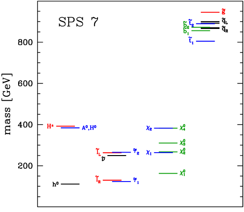
Figure 2: The SUSY mass spectrum of the benchmark point corresponding to SPS 7 [11].

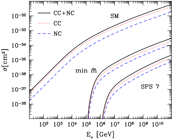
Figure 3: The charged (red dotted) and neutral (blue dashed) current cross section for neutrino-nucleon scattering compared to the chargino and neutralino exchange for the SPS 7 benchmark point and a scenario with light squark masses of 300 GeV.

The corresponding mass spectrum calculated by SoftSusy 2.0.4 [15] is shown in Fig. 2. The other spectrum (denoted by “min $\widetilde{m}$” in the following) consists of light charginos, neutralinos and sleptons at 100 GeV and squarks at 300 GeV. It is not motivated by any particular SUSY breaking scenario, but oriented at current experimental limits, in order to give an impression of what can be obtained in a very optimistic scenario.

The resulting neutrino-nucleon cross sections are shown in Fig. 3, compared to the SM contribution from $W$ and $Z$ exchange. Here and in the following computations we have used the CTEQ6D parton distribution functions [16]. The contribution to the cross sections from charged currents is about twice as large as the one from neutral currents.

In Eqs. (1a)–(1d), we have neglected family mixings and contributions proportional to Yukawa couplings. We have taken into account the exchange of the heavier neutralinos and charginos, since generically their contribution to the cross sections is large and can even dominate. At the SPS 7 benchmark point we consider, assuming equal neutralino masses turns out to be a rather good approximation that helps simplify analytical calculations. Nevertheless, we use the exact expressions in the numerical calculations discussed in the following.

3 NLSP Propagation

The squarks and sleptons produced in the interactions discussed in the previous section promptly decay into stau NLSPs. Now, we discuss the survival probability of the latter after propagation towards the Cherenkov light detector. The corresponding effective detection volume is limited by energy loss and decay.

3.1 Energy Loss

In the case of the muon, the mean energy loss per column depth $z$, measured in $\text{g}\,\text{cm}^{-2}$, is given as

$$-\left\langle\frac{{\rm d}E_{\mu}}{{\rm d}z}\right\rangle\approx\alpha_{\mu}+\beta_{\mu}E_{\mu}.$$ (1b)

Here, $\alpha_{\mu}$ is determined by ionization effects and $\beta_{\mu}$ accounts for bremsstrahlung, pair-production, and photohadronic processes. In general, these coefficients are weakly energy dependent. For our purpose, it is sufficient to approximate their values by constants, $\alpha_{\mu}\approx 2\cdot 10^{-3}\ \text{GeV}\,\text{cm}^{2}\,\text{g}^{-1}$ and $\beta_{\mu}\approx 4\cdot 10^{-6}\ \text{cm}^{2}\,\text{g}^{-1}$. For muons above a critical energy $E_{\mu}^{\text{cr}}=\alpha_{\mu}/\beta_{\mu}\approx 500$ GeV, radiative energy losses dominate, which are proportional to the energy itself. Hence, Eq. (1b) can be used to determine the muon energy if $E_{\mu}\gg E^{\text{cr}}_{\mu}$. We will take this critical energy as an effective cut-off in the following since the detection efficiency becomes very small below [17]. The range of a muon is then given as

$$R(E_{\mu},E_{\mu}^{\text{cr}})\approx\frac{1}{\beta_{\mu}}\ln\left(\frac{\alpha_{\mu}+\beta_{\mu}E_{\mu}}{\alpha_{\mu}+\beta_{\mu}E_{\mu}^{\text{cr}}}\right).$$ (1c)

In the case of a stau, the radiative term in Eq. (1b) is suppressed, since $\beta_{\widetilde{\tau}}$ satisfies $\beta_{\widetilde{\tau}}m_{\widetilde{\tau}}\approx\beta_{\mu}m_{\mu}$. At large energies this gives an increase of the stau range compared to that of the muon by the mass ratio $m_{\widetilde{\tau}}/m_{\mu}$. In the following we will use the results of [8] for the range of the stau.

3.2 Decay

The lifetime of the stau NLSP can be very long, since its decay into the gravitino LSP can proceed only gravitationally. The corresponding decay length $L$ for relativistic staus, in units of the Earth’s diameter $2R_{\oplus}$, is (e.g. [19])

$$\bigg{(}\frac{L}{2R_{\oplus}}\bigg{)}\approx\bigg{(}\frac{m_{\tilde{\tau}}}{100\ \text{GeV}}\bigg{)}^{-6}\bigg{(}\frac{m_{3/2}}{400\ \text{keV}}\bigg{)}^{2}\bigg{(}\frac{E_{\tilde{\tau}}}{500\ \text{GeV}}\bigg{)}.$$ (1d)

The minimal stau energy we consider is about 500 GeV, corresponding to the critical energy of the muons. Hence, staus with a mass not much larger than 100 GeV will always reach the detector, if the gravitino is heavier than 400 keV. In this case, the gravitino is a viable candidate for the dark matter [20]. Constraints from big bang nucleosynthesis and the cosmic microwave background yield an upper limit on the gravitino mass between 10 and 100 GeV [21]. Masses in the lower part of the allowed region are typical for models with gauge-mediated SUSY breaking, while masses of some tens of GeV can occur in gravity and gaugino mediation (for a review, cf. e.g. [22]).

4 Detection Rate at Neutrino Telescopes

There are several Cherenkov light based neutrino telescopes currently operating or under construction in the Antarctic (AMANDA [23, 24] and IceCube [10]), in Lake Baikal [25, 26], and in the Mediterranean (ANTARES [27], NEMO [28], and NESTOR [29]). The total flux of staus through a detector is proportional to the initial flux of high energy cosmic neutrinos $F$, attenuated inside the Earth according to the total inelastic neutrino-nucleon cross section $\sigma_{\nu N}$. A slepton (squark) produced with an energy $E_{\widetilde{l}}$ ($E_{\widetilde{q}}$) and a cross section $\sigma^{\rm SUSY}_{\nu N}$ will promptly decay into a stau which looses energy by radiative processes according to Eq. (1b) and reaches the detector with energy $E_{\widetilde{\tau}}$. The flux of staus per area $A$, time $t$, steradian $\Omega$, and energy $E_{\widetilde{\tau}}$ is then given as

$$\qquad\frac{{\rm d}^{4}N}{{\rm d}t\,{\rm d}A\,{\rm d}\Omega\,{\rm d}E_{\widetilde{\tau}}}\approx\int\limits_{0}^{z_{\text{tot}}}\frac{{\rm d}z}{m_{\text{p}}}\int\limits_{E_{\text{min}}}^{E_{\text{max}}}\!\!{\rm d}E_{\nu}\sum\limits_{i=\widetilde{l},\widetilde{q}}\,\left|\frac{{\rm d}E_{i}}{{\rm d}E_{\widetilde{\tau}}}\right|\frac{{\rm d}\sigma^{\rm\scriptscriptstyle SUSY}_{\nu N}}{{\rm d}E_{i}}\exp\left(-\frac{z}{m_{\text{p}}}\sigma_{\nu N}\right)F(E_{\nu}).$$ (1e)

Here, $m_{\text{p}}$ is the proton mass, and the column depth $z$ of the Earth is related to $l$, the distance to the detector in the line of sight, as $-{\rm d}z=\rho(l,\theta){\rm d}l$. For the calculation of the total column depth of the Earth we use the density profile given in [30] and a detector center at 1.9 km depth, as it is the case for IceCube. The measure $|{\rm d}E_{i}/{\rm d}E_{\widetilde{\tau}}|$ takes into account the energy loss of a stau as well as the mean energy fraction it carries in the decay of the initial slepton or squark. For the SPS 7 benchmark point we have estimated $\langle E_{\widetilde{\tau}}\rangle\approx 0.3E_{\widetilde{q}}$ and $\langle E_{\widetilde{\tau}}\rangle\approx 0.5E_{\widetilde{l}}$, respectively. For the optimistic scenario with light sparticles this changes to $\langle E_{\widetilde{\tau}}\rangle\approx 0.5E_{\widetilde{q}}$ and $\langle E_{\widetilde{\tau}}\rangle\approx E_{\widetilde{l}}$, respectively.

For the flux of high energy cosmic neutrinos, we adopt the Waxman-Bahcall (WB) flux, $E_{\nu}^{2}F(E_{\nu})\approx 2\cdot 10^{-8}\ \text{cm}^{-2}\,\text{s}^{-1}\,\text{sr}^{-1}\,\text{GeV}$ per flavor [12]. This flux is based on the assumption that the observed ultra high energy cosmic rays are protons from extragalactic astrophysical acceleration sites. In these violent environments protons, neutrinos, and gamma rays are produced with comparable luminosities. As a maximal neutrino energy we take $10^{10}$ GeV. We have checked that an increase of this cut-off does not affect our results.

The analysis of particle tracks observed in neutrino telescopes is calibrated for muons. Their energy $E_{\mu}$ can be reconstructed by the energy loss $\Delta E$ per column depth $\Delta z$ and Eq. (1b). This is appropriate for muons with energies above the critical energy $E^{\text{cr}}_{\mu}=\alpha_{\mu}/\beta_{\mu}\approx 500\ \text{GeV}$. A high-energy stau with energy $E_{\widetilde{\tau}}$ will deposit a much smaller energy fraction in the detector compared to a muon with the same energy, due to the reduced radiative energy loss. This has two effects. Firstly, the critical energy of a stau $E_{\widetilde{\tau}}^{\text{cr}}=\alpha_{\widetilde{\tau}}/\beta_{\widetilde{\tau}}\approx(m_{\widetilde{\tau}}/m_{\mu})E^{\text{cr}}_{\mu}$ is much higher compared to the muons. Secondly, due to the calibration of the detector, high-energy staus will be detected as muons with reduced energy $E_{\text{d}}\approx(m_{\mu}/m_{\widetilde{\tau}})E_{\widetilde{\tau}}$. Note that this correctly identifies the boost factor of the particle $\gamma=E_{\widetilde{\tau}}/m_{\widetilde{\tau}}=E_{\text{d}}/m_{\mu}$. Also the Cherenkov angle is consistently identified by $\cos\theta_{C}\propto(1-1/\gamma^{2})^{-1/2}$. For that reason, we will present our results in Fig. 4 in terms of the detected energy $E_{\text{d}}$. Of course, the total number of events does not change by this recalibration. Note that the critical energy for the stau has the same value for muons and staus in terms of the detected energy. For completeness, we show our results also in terms of the neutrino energy.

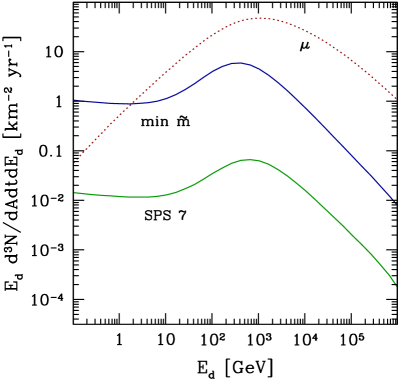
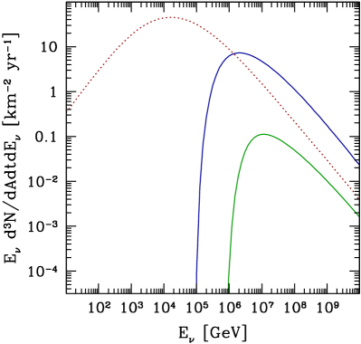
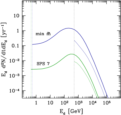
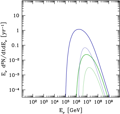
Figure 4: Expected fluxes and event rates for the example of IceCube and the Waxman-Bahcall neutrino flux [12]. The results are shown in terms of the detected energy $E_{\text{d}}$ (left panels) and the neutrino energy $E_{\nu}$ (right panels). We have used a SUSY mass spectrum with light squarks of 300 GeV (blue upper solid) as well as the one from the benchmark point corresponding to SPS 7 (green lower solid).
Upper panels: Fluxes of upward-going muons (red dotted) and staus (solid). For optimistic SUSY scenarios the spectrum of staus may dominate over the flux of muons at large neutrino energies (right panel). However, the detected spectrum of staus will be subdominant (left panel) due to the detector calibration explained in the text.
Lower panels: Rates of parallel-stau events for an energy cut-off at $E^{\text{cr}}_{\mu}=\alpha_{\mu}/\beta_{\mu}$ (thick solid) and at $E^{\text{cr}}_{\widetilde{\tau}}=\alpha_{\widetilde{\tau}}/\beta_{\widetilde{\tau}}=(m_{\widetilde{\tau}}/m_{\mu})E^{\text{cr}}_{\mu}$ (thin solid), respectively.

4.1 One-Muon vs. One-Stau Events

The upper panels of Fig. 4 show the differential fluxes of muons and staus through the IceCube detector. The calculation of the total rate of events requires the knowledge of the detection efficiency of the corresponding particle depending on its energy and direction. This is usually combined with the cross sectional area of the detector as an effective area $A_{\text{eff}}$. The IceCube Collaboration has determined the effective area $A^{\mu}_{\text{eff}}(\cos\theta,E_{\mu})$ for upward-going muons by Monte-Carlo simulations in [17]. The angle-averaged values are shown in Tab. 1 together with the expected rates of muon events for the WB flux. The expected rates are in good agreement with those quoted in [17], if one takes into account the different normalizations of the initial neutrino fluxes.

Despite the fact that the staus are produced in pairs, they may also produce one-stau events, for example if one particle of the pair misses the detector. These are indistinguishable from one-muon events, at least for high energies. A very conservative upper bound on the rate of one-stau events is given by the total rate of staus computed from Eq. (1e) and a detection efficiency $A^{\widetilde{\tau}}_{\text{eff}}(E_{\widetilde{\tau}})\approx A^{\mu}_{\text{eff}}(E_{\text{d}})$. This upper bound is also shown in Tab. 1 and Fig. 4 for the two different SUSY mass spectra. It shows that in the fiducial energy region one-stau events are subdominant compared to the flux of muons, even for the most optimistic case of very light squarks with masses around 300 GeV. This seems to be generic, independent of the initial high-energy cosmic neutrino flux, as we have checked. Hence, the total rate of one-particle events can be used for reconstructing the neutrino flux without taking into account the contributions from NLSPs. This decouples the analysis of the extra-galactic neutrino flux from the search for parallel-stau events, to which we turn now.

• $E_{\text{d}}$ [GeV]	$(\,10\,,\,10^{2}\,)$	$(\,10^{2}\,,\,10^{3}\,)$	$(\,10^{3}\,,\,10^{4}\,)$	$(\,10^{4}\,,\,10^{5}\,)$	$(\,10^{5}\,,10^{6}\,)$
  $A^{\mu}_{\rm eff}$ [${\rm km}^{2}$]	$0.1$	$0.6$	$0.8$	$1.0$	$1.2$
  $N_{\mu}$	3	60	100	80	20
  $N_{\widetilde{\tau}}$ (minimal $\widetilde{m}$)	$<0.9$	$<10$	$<6$	$<0.9$	$<0.1$
  $N_{\widetilde{\tau}}$ (SPS 7)	$<0.009$	$<0.1$	$<0.1$	$<0.02$	$<0.003$

Table 1: The expected number of muon and stau events for a one year observation at IceCube, assuming the Waxman-Bahcall neutrino flux per flavor, $E_{\nu}^{2}F(E_{\nu})\approx 2\cdot 10^{-8}\ \text{cm}^{-2}\,\text{s}^{-1}\,\text{sr}^{-1}\,\text{GeV}$ [12]. The effective areas of IceCube have been calculated by Monte-Carlo simulations and are given in [17].

4.2 Rate of Parallel-Stau Events

The detection efficiency of stau pairs, i.e. coincident parallel tracks, depends on the energies and directions of the staus, as in the case of single events, and also on their separation. As a detailed Monte-Carlo simulation is beyond the scope of this study, we will use a simple approximation for the resulting angle-averaged effective area in the following. Firstly, we introduce a low energy cut-off for the detectable stau energy. As examples, we use the critical energies of the muon and of the stau. Secondly, we assume that the observatory can identify an event of coincident parallel stau tracks, if they are separated by more than 50 m [31] and less than 1 km. Here, we approximate the opening angle by the angle between sleptons and squarks in the laboratory frame. If the pair event survives these cuts, we assume an effective area of $1\ \text{km}^{2}$ for its detection.

The lower panels of Fig. 4 show the expected rates of these pair events for the two SUSY scenarios. Since the staus of a pair have different energies, we show the average of the corresponding spectra. Note that a higher energy threshold in the detector does also affect the range of the second stau. This has an effect on the pair rates even if one stau is above the threshold as can be seen in the plots. The main reason for the suppression at large energies $E_{\text{d}}$ is the requirement that the opening angle of the staus be compatible with the restriction on the separation. On the other hand, the distance of the interaction point from the detector has to be smaller than the corresponding range of the second stau. This mainly causes the reduction at small energies $E_{\text{d}}$. For the Waxman-Bahcall neutrino flux and one year of observation at IceCube, we predict about 0.09 pair events for the benchmark point corresponding to SPS 7 and about 5 events for our toy model with light sparticle masses. This calculation assumes an effective low-energy cut-off at $E^{\text{cr}}_{\mu}$. We also show the effect of increasing the cut-off to $E^{\text{cr}}_{\widetilde{\tau}}=(m_{\widetilde{\tau}}/m_{\mu})E^{\text{cr}}_{\mu}$. This might be necessary due to the reduced radiative energy loss of the stau. Our expectations are then reduced to 0.009 and 0.2 events, respectively. Currently, the IceCube Collaboration quotes an upper limit at $90\%$ confidence level of $E_{\nu}^{2}F(E_{\nu})\lesssim 3\cdot 10^{-7}\ \text{cm}^{-2}\,\text{s}^{-1}\,\text{sr}^{-1}\,\text{GeV}$ per flavor for the diffuse flux of cosmic neutrinos [32]. This is approximately one order of magnitude above the Waxman-Bahcall flux taken for our calculation. If the cosmic neutrino flux does not lie much below this limit, the predicted event rates will increase by a factor 10, giving up to 50 pair events for the optimistic SUSY mass spectrum.

The expected background of parallel muon pair events from random coincidences is bounded from above by the number of muons arriving within a (generous) time-window of $1\ \mu\text{s}$. Even this is several orders of magnitude below the stau pair event rate,

$$\frac{N_{\mu+\mu}(E)}{N_{\mu}(E)}\lesssim\frac{1}{2}\text{min}\Bigg{(}1\,;{1\ \mu\text{s}}\cdot\frac{{\rm d}N_{\mu}}{{\rm d}t}\Bigg{)}\sim\mathcal{O}(10^{-12}).$$ (1f)

However, double muon events from processes like $\nu_{\mu}+N\rightarrow\mu^{-}+\pi^{+}+X\rightarrow\mu^{-}+\mu^{+}+\nu_{{\mu}}+X$ are expected to be more likely. We expect that these contributions are still subdominant compared to stau pairs due to meson-nucleon interactions in the Earth. This should be studied in more detail in the future.

5 Summary and Discussion

High energy cosmic neutrinos collide with matter in the Earth at center of mass energies beyond the capability of any earth-bound experiment. The attempt to measure the cosmic ray fluxes in various observatories is therefore tightly connected to extrapolations of the SM interactions of these particles to very high energies. Besides, one can look for deviations from the SM predictions for the strength of the interactions or even for new particles.

In this paper, we have examined the question whether neutrino telescopes could play a significant role in the discovery and study of supersymmetric extensions of the SM with a gravitino LSP and a long-lived stau NLSP. In these models, neutrino-nucleon interactions can produce pairs of staus which show up as parallel tracks in the detector [7].

We have argued that events with a single stau in the detector are virtually indistinguishable from muon events at high energies. However, the reduced energy loss of staus in matter, which increases the effective volume, reduces also the detection efficiency in the telescope. As a result, single stau events play only a subdominant role compared to muon events. Consequently, the reconstruction of the initial high-energy neutrino flux from the total rate of muon-like events can proceed assuming SM interactions alone.

If the superpartner masses are close to their experimental limits and if the cosmic neutrino flux is also close to its current experimental bound, we expect up to 50 pair events per year in a cubic kilometer detector such as IceCube, with negligible background. Less favorable event rates are obtained for a less optimistic cut-off in the stau energy or for SUSY mass spectra of commonly used scenarios for SUSY breaking, mainly because the squarks are significantly heavier.

If the gravitino mass is larger than 400 keV, as we have assumed, the stau decay length is larger than the Earth’s diameter. Thus, the spectrum is independent of the gravitino mass. For lighter gravitinos, the rate of stau pairs will drop starting at the low-energy end of the spectrum. Therefore, it might be possible to obtain information about the gravitino mass, if the spectrum is measured very accurately and if the superpartner masses are known. However, with the small number of pair events we find, this appears challenging.

References

References

- [1] A. Brandenburg, L. Covi, K. Hamaguchi, L. Roszkowski, and F. D. Steffen, Phys. Lett. B617, 99 (2005), hep-ph/0501287.
- [2] T. Jittoh, J. Sato, T. Shimomura, and M. Yamanaka, Phys. Rev. D73, 055009 (2006), hep-ph/0512197.
- [3] W. Buchmüller, K. Hamaguchi, M. Ratz, and T. Yanagida, Phys. Lett. B588, 90 (2004), hep-ph/0402179.
- [4] K. Hamaguchi, Y. Kuno, T. Nakaya, and M. M. Nojiri, Phys. Rev. D70, 115007 (2004), hep-ph/0409248.
- [5] J. L. Feng and B. T. Smith, Phys. Rev. D71, 015004 (2005), hep-ph/0409278.
- [6] K. Hamaguchi and A. Ibarra, JHEP 02, 028 (2005), hep-ph/0412229.
- [7] I. Albuquerque, G. Burdman, and Z. Chacko, Phys. Rev. Lett. 92, 221802 (2004), hep-ph/0312197.
- [8] M. H. Reno, I. Sarcevic, and S. Su, Astropart. Phys. 24, 107 (2005), hep-ph/0503030.
- [9] X.-J. Bi, J.-X. Wang, C. Zhang, and X. Zhang, Phys. Rev. D70, 123512 (2004), hep-ph/0404263.
-
[10]
IceCube, J. Ahrens et al.,
Nucl. Phys. Proc. Suppl. 118, 388 (2003), astro-ph/0209556,
http://icecube.wisc.edu/. - [11] B. C. Allanach et al., Eur. Phys. J. C25, 113 (2002), hep-ph/0202233.
- [12] E. Waxman and J. N. Bahcall, Phys. Rev. D59, 023002 (1999), hep-ph/9807282.
- [13] J. Rosiek, Phys. Rev. D41, 3464 (1990), Erratum hep-ph/9511250.
- [14] A. Denner, H. Eck, O. Hahn, and J. Küblbeck, Nucl. Phys. B387, 467 (1992).
- [15] B. C. Allanach, Comput. Phys. Commun. 143, 305 (2002), hep-ph/0104145.
- [16] J. Pumplin et al., JHEP 07, 012 (2002), hep-ph/0201195.
- [17] IceCube, J. Ahrens et al., Astropart. Phys. 20, 507 (2004), astro-ph/0305196.
- [18] J. Beacom, private communication.
- [19] G. F. Giudice and R. Rattazzi, Phys. Rept. 322, 419 (1999), hep-ph/9801271.
- [20] H. Pagels and J. R. Primack, Phys. Rev. Lett. 48, 223 (1982).
- [21] D. G. Cerdeño, K.-Y. Choi, K. Jedamzik, L. Roszkowski, and R. Ruiz de Austri, (2005), hep-ph/0509275.
- [22] D. J. H. Chung et al., Phys. Rept. 407, 1 (2005), hep-ph/0312378.
-
[23]
AMANDA, E. Andres et al.,
Astropart. Phys. 13, 1 (2000), astro-ph/9906203,
http://amanda.wisc.edu/. - [24] AMANDA, J. Ahrens et al., Phys. Rev. Lett. 92, 071102 (2004), astro-ph/0309585.
-
[25]
BAIKAL, I. A. Belolaptikov et al.,
Astropart. Phys. 7, 263 (1997),
http://www-zeuthen.desy.de/baikal/baikalhome.html. - [26] Baikal, V. A. Balkanov et al., Phys. Atom. Nucl. 63, 951 (2000), astro-ph/0001151.
-
[27]
ANTARES, E. Aslanides et al.,
(1999), astro-ph/9907432,
http://antares.in2p3.fr/. - [28] NEMO, P. Piattelli, Nucl. Phys. Proc. Suppl. 143, 359 (2005).
-
[29]
NESTOR, P. K. F. Grieder,
Nuovo Cim. 24C, 771 (2001),
http://www.nestor.org.gr/. - [30] R. Gandhi, C. Quigg, M. H. Reno, and I. Sarcevic, Astropart. Phys. 5, 81 (1996), hep-ph/9512364.
- [31] C. Spiering (IceCube Collaboration), private communication.
- [32] IceCube, M. Ackermann et al., Nucl. Phys. Proc. Suppl. 145, 319 (2005).