Electroweak radiative corrections to the Higgs-boson production in association with $Z^{0}$-boson pair at $e^{+}e^{-}$ colliders

Abstract

We present the full ${\cal O}(\alpha_{{ew}})$ electroweak radiative corrections to the Higgs-boson production in association with $Z^{0}$-boson pair at an electron-positron linear collider(LC) in the standard model. We analyze the dependence of the full one-loop corrections on the Higgs-boson mass $m_{H}$ and colliding energy $\sqrt{s}$. We find that the corrections significantly suppress the Born cross section, and the ${\cal O}(\alpha_{{ew}})$ electroweak radiative corrections are generally between $1.0\%$ and $-15\%$ in our chosen parameter space, which should be taken into consideration in the future precise experiments.

PACS: 12.15.Lk, 14.80.Bn, 14.70.Hp,11.80.Fv

I Introduction

One of the most important missions of the future high energy experiments is to search for scalar Higgs-boson, which is believed to be responsible for the breaking of the electroweak symmetry and the generation of masses for the fundamental particles in the standard model(SM)[1, 2]. Until now the Higgs-boson hasn’t been observed yet, only LEP II experiment provides a lower bound of 114.4 GeV[3] and an upper bound of 260 GeV[4] for the mass of the SM Higgs-boson at $95\%$ confidence level. People believe that with the help of future high energy colliders, such as the CERN large hadron collider(LHC), and the linear colliders, TESLA, NLC, JLC and CERN CLIC, the existence of the Higgs-boson would be proved or excluded in the experiments.

As far as we know, the present precise experimental data have shown an excellent agreement with the predictions of the SM except the Higgs sector[5]. These data strongly constrain the couplings of the gauge-boson to fermions ($g_{Zf\bar{f}}$ and $g_{Wf\bar{f^{\prime}}}$), and gauge bosons self-couplings, but say little about the couplings between Higgs-boson and gauge bosons, which wouldn’t exist if the corresponding scalar field has no vacuum expectation value. In order to reconstruct Higgs potential, the precise predictions for Higgs couplings, which include Yukawa couplings, the couplings of Higgs to gauge bosons and the Higgs self-couplings, are necessary. At an $e^{+}e^{-}$ linear collider with $\sqrt{s}\simeq 300-500~{}GeV$, Higgs-boson with an intermediate mass value would be produced mainly via the Higgs strahlung process $e^{+}e^{-}\to Z^{0}H^{0}~{}$, and the coupling of Higgs-boson to $Z$-bosons is probed best in the measurement of the cross sections of the Higgs strahlung process $e^{+}e^{-}\to Z^{0}H^{0}~{}$and the $WW/ZZ$ fusion processes $e^{+}e^{-}\to H^{0}\nu\bar{\nu}$ and $e^{+}e^{-}\to H^{0}e^{+}e^{-}$. In Refs.[6], it shows that the coupling $g_{ZZH}$ can be determined at a few percent level for a $120~{}GeV$ Higgs-boson with an integrated luminosity of $500~{}fb^{-1}$ from the production cross section through the process $e^{+}e^{-}\to Z^{0}H^{0}~{}$. There is another class of processes which is interesting for the studies of Higgs physics at linear collider called Higgs-boson production in association with a pair of final particles which can be used to test the Yukawa couplings, couplings between Higgs-boson and gauge bosons, and Higgs self-couplings. For example, $e^{+}e^{-}\to Z^{0}Z^{0}H^{0}~{}$process is not only an important process in probing $g_{ZZH}$, but also possible to provide further tests for the quadrilinear couplings(such as C-violating $HZZZ$ or $H\gamma ZZ$), which do not exist at tree-level in the SM, because these quadrilinear couplings would induce deviations from the SM predicted observables[7]. We believe that once the neutral Higgs-boson is discovered and its mass is determined, the double $Z^{0}$-bosons production through $e^{+}e^{-}\to Z^{0}Z^{0}H^{0}~{}$process may provide the detail information of the coupling between Higgs-boson and $Z^{0}$ gauge bosons, which directly reflects the role of the Higgs-boson in electroweak symmetry breaking. Moreover, a theoretical accurate estimate of this class of processes is essential, since $e^{+}e^{-}\to Z^{0}Z^{0}H^{0}~{}$process could be potential backgrounds for possible new physics.

There have been already some theoretical works in investigating the Yukawa couplings, the Higgs self-couplings and Higgs couplings with gauge boson pair in the SM at LC, for example, the calculations of the NLO QCD and one-loop electroweak corrections to the $e^{+}e^{-}\to t\bar{t}H^{0}$ process in Refs.[8, 9, 10, 11] and $\gamma\gamma\to t\bar{t}H^{0}$ process in Ref.[12] in probing Yukawa coupling, the one-loop electroweak corrections to the process $e^{+}e^{-}\to H^{0}H^{0}Z^{0}~{}$in Ref.[13, 14] for testing Higgs self-coupling. The Higgs productions in association with vector gauge bosons($e^{+}e^{-}\to H^{0}W^{+}W^{-}$, $e^{+}e^{-}\to H^{0}Z^{0}Z^{0}$ and $e^{+}e^{-}\to H^{0}Z^{0}\gamma$) in the SM for testing the couplings between Higgs-boson and gauge bosons were studied at the tree-level in Ref.[7]. In this work we calculate the full one-loop electroweak corrections to the process $e^{+}e^{-}\to Z^{0}Z^{0}H^{0}~{}$in the SM. The paper is arranged as follows: In Section II we give the analytical calculations of the Born cross section and the full ${\cal O}(\alpha_{ew})$ electroweak corrections to the $e^{+}e^{-}\to Z^{0}Z^{0}H^{0}~{}$process. In Section III we present some numerical results, and finally a short summary is given.

II Calculation of $e^{+}e^{-}\to Z^{0}Z^{0}H^{0}~{}$

The tree-level Feynman diagrams contributing to the process $e^{+}e^{-}\to Z^{0}Z^{0}H^{0}~{}$in the frame of the SM are depicted in Fig.1. Due to the fact that the Yukawa coupling strength between Higgs/Goldstone and fermions is proportional to the fermion mass, it is reasonable to neglect the contributions of the Feynman diagrams which include $H^{0}-e^{+}-e^{-}$ or $G^{0}-e^{+}-e^{-}$ coupling.

Figure 1: The tree-level Feynman diagrams for the process $e^{+}e^{-}\to Z^{0}Z^{0}H^{0}~{}$.

We calculated the Born cross section of the process $e^{+}e^{-}\to Z^{0}Z^{0}H^{0}~{}$by using ’t Hooft-Feynman gauge and unitary gauge to check the gauge invariance by adopting $FeynArts~{}3.2$ package[15], and got the coincident numerical results. The electroweak one-loop Feynman diagrams can be classified into self-energy, triangle, box and pentagon diagrams. As a representative selection, the pentagon diagrams are depicted in Fig.2. Their corresponding amplitudes may involve five point tensor integrals up to rank 4. In the amplitude calculation of the process $e^{+}e^{-}\to Z^{0}Z^{0}H^{0}~{}$involving one-loop contributions, we create all the tree-level, one-loop Feynman diagrams and their relevant amplitudes in the ’t Hooft-Feynman gauge by using $FeynArts~{}3.2$, and the Feynman amplitudes are subsequently reduced by $FormCalc~{}4$ [16]. Our renormalization procedure is implemented in these packages. The numerical calculation of the two-, three- and four-point integral functions are done by using FF package[17]. The implementations of the scalar and the tensor five-point integrals are done exactly by using the Fortran programs as used in our previous works on $e^{+}e^{-}\to t\bar{t}H^{0}$ and $e^{+}e^{-}\to Z^{0}H^{0}H^{0}$ processes[9, 13] with the approach presented in Ref.[18].

Figure 2: The pentagon Feynman diagrams for the process $e^{+}e^{-}\to Z^{0}Z^{0}H^{0}~{}$.

The ${\cal O}(\alpha_{ew})$ virtual electroweak correction to the $e^{+}e^{-}\to Z^{0}Z^{0}H^{0}~{}$process can be expressed as:

$$\sigma_{\rm virtual}=\sigma_{\rm tree}\delta_{\rm virtual}=\frac{1}{2}\frac{(2\pi)^{4}}{2|\vec{p}_{1}|\sqrt{s}}\int d\Phi_{3}\overline{\sum_{spin}}Re({\cal M}_{\rm tree}{\cal M}^{{\dagger}}_{\rm virtual})$$ (1)

where the first factor $\frac{1}{2}$ comes from the two identical $Z^{0}$-bosons in the final state, $\vec{p}_{1}$ is the momentum of the incoming positron in the center of mass system(c.m.s.), ${\rm d}\Phi_{3}$ is the three-body phase space element, and the bar over summation recalls averaging over initial spins [19]. $\sigma_{\rm tree}$ and ${\cal M}_{\rm tree}$ are the cross section and amplitude at the tree-level for process $e^{+}e^{-}\to Z^{0}Z^{0}H^{0}~{}$, respectively. ${\cal M}_{\rm virtual}$ is the renormalized amplitude from all the electroweak one-loop Feynman diagrams and the corresponding counterterms. The related renormalized quantities and renormalization constants are defined as in Ref.[22], and can be evaluated by using the corresponding equations shown in this reference.

The total unrenormalized amplitude corresponding to all the one-loop Feynman diagrams contains both ultraviolet (UV) and infrared (IR) divergences. To regularize the UV divergences in loop integrals, we adopt the dimensional regularization scheme [20] in which the dimensions of spinor and space-time manifolds are extended to $D=4-2\epsilon$. And we adopt the on-mass-shell (OMS) scheme [21, 22] to renormalize the relevant fields. All the tensor coefficients of the one-loop integrals can be calculated by using the reduction formulae presented in Refs.[23, 24]. We check the UV finiteness of our results of the whole contributions of the virtual one-loop diagrams and counterterms both analytically and numerically by regularizing the IR divergence with a fictitious photon mass. As we expect, the UV divergence contributed by virtual one-loop diagrams can be cancelled by that contributed from the counterterms exactly.

The soft IR divergence in the process $e^{+}e^{-}\to Z^{0}Z^{0}H^{0}~{}$is originated from virtual photonic corrections, which can be exactly cancelled by adding the real photonic bremsstrahlung corrections to this process in the soft photon limit. In the real photon emission process

$$e^{+}(p_{1})+e^{-}(p_{2})\rightarrow Z^{0}(k_{1})+Z^{0}(k_{2})+H^{0}(k_{3})+\gamma(k_{\gamma}),$$ (2)

a real photon radiates from the electron/positron, and can have either soft or collinear nature. The collinear singularity is regularized by keeping electron(positron) mass. We use the general phase-space-slicing (PSS) method [25] to isolate the soft photon emission singularity in the real photon emission process. In the PSS method, the bremsstrahlung phase space is divided into singular and non-singular regions, and the cross section of the real photon emission process (2) is decomposed into soft and hard terms

$$\sigma_{{\rm real}}=\sigma_{{\rm soft}}+\sigma_{{\rm hard}}=\sigma_{\rm tree}(\delta_{{\rm soft}}+\delta_{{\rm hard}}).$$ (3)

where the ’soft’ and ’hard’ describe the energy of the radiated photon. The energy $E_{\gamma}$ of the radiated photon in the center of mass system(c.m.s.) frame is considered soft and hard if $E_{\gamma}\leq\Delta E$ and $E_{\gamma}>\Delta E$, respectively. Both $\sigma_{{\rm soft}}$ and $\sigma_{{\rm hard}}$ depend on the arbitrary soft cutoff $\Delta E/E_{b}$, where $E_{b}=\sqrt{s}/2$ is the electron beam energy in the c.m.s. frame, but the total cross section of the real photon emission process $\sigma_{{\rm real}}$ is cutoff independent. Since the soft cutoff $\Delta E/E_{b}$ is taken to be a small value in our calculations, the terms of order $\Delta E/E_{b}$ can be neglected and the soft contribution can be evaluated by using the soft photon approximation analytically [21, 22, 26]

$${\rm d}\sigma_{{\rm soft}}=-{\rm d}\sigma_{{\rm tree}}\frac{\alpha_{ew}}{2\pi^{2}}\int_{|\vec{k}_{\gamma}|\leq\Delta E}\frac{{\rm d}^{3}k_{\gamma}}{2E_{\gamma}}\left(\frac{p_{1}}{p_{1}\cdot k_{\gamma}}-\frac{p_{2}}{p_{2}\cdot k_{\gamma}}\right)^{2}.$$ (4)

As shown in Eq.(4), the soft contribution has an IR singularity at $m_{\gamma}=0$, which can be cancelled exactly with that from the virtual photonic corrections. Therefore, $\sigma_{{\rm virtual}+{\rm soft}}$, the sum of the ${\cal O}(\alpha_{ew}^{4})$ virtual and soft photon emission cross section corrections, is independent of the fictitious small photon mass $m_{\gamma}$. The hard contribution, which is UV and IR finite, is computed by using the Monte Carlo technique. Finally, the corrected cross section for the $e^{+}e^{-}\to Z^{0}Z^{0}H^{0}~{}$process up to the order of ${\cal O}(\alpha^{4}_{ew})$ is obtained by summing the ${\cal O}(\alpha^{3}_{ew})$ Born cross section $\sigma_{\rm tree}$, the ${\cal O}(\alpha^{4}_{ew})$ virtual cross section $\sigma_{\rm virtual}$, and the ${\cal O}(\alpha^{4}_{ew})$ cross section of the real photon emission process (2), i.e.,

$$\sigma_{{\rm total}}=\sigma_{{\rm tree}}+\sigma_{{\rm virtual}}+\sigma_{{\rm real}}=\sigma_{{\rm tree}}\left(1+\delta_{{\rm total}}\right),$$ (5)

In order to analyze the origins of the one-loop electroweak corrections clearly, we organize the full one-loop electroweak corrections to the process $e^{+}e^{-}\to Z^{0}Z^{0}H^{0}~{}$in two parts, the QED correction part and the weak correction part. The QED part comes from the QED virtual correction and the real photon emission correction. The QED virtual correction involves the contributions from the one-loop diagrams with virtual photon exchange in the loop. For some counterterms involved in the QED contribution, we only have to take into account purely photonic contribution to the wave function renormalization constants of the electron/positron. The rest of the total virtual electroweak corrections is called the weak correction part. With such definitions of the origins of the radiative correction we can divide the full one-loop electroweak corrected total cross section in following form:

$$\sigma_{{\rm total}} = \sigma_{{\rm tree}}+\sigma_{{\rm virtual+soft}}+\sigma_{{\rm hard}}=\sigma_{{\rm tree}}+\sigma^{QED}_{{\rm virtual+soft}}+\sigma^{QED}_{{\rm hard}}+\sigma^{W}$$ (6)

$$= \sigma_{{\rm tree}}\left(1+\delta^{QED}+\delta^{W}\right)=\sigma_{{\rm tree}}\left(1+\delta_{{\rm total}}\right),$$

where $\sigma_{{\rm virtual+soft}}$ is the cross section correction contributed by the virtual electroweak one-loop diagrams and the soft photon emission process, $\sigma^{QED}_{{\rm virtual+soft}}$, $\sigma^{QED}_{{\rm hard}}$ and $\sigma^{W}$ are the corrections from the QED contributions including only the photonic one-loop diagrams and the soft photon emission process, the hard photon emission process and the weak virtual contribution, separately. $\delta^{QED}_{{\rm virtual+soft}}$ is the relative correction including the contributions of QED one-loop diagrams and the soft photon emission process. $\delta^{QED}$, $\delta^{W}$ and $\delta_{{\rm total}}$ are the relative corrections contributed by the QED correction part, the weak correction part and the total electroweak correction, respectively.

III Numerical Results and Discussions

In our numerical calculation, we adopt the $\alpha_{ew}$-scheme, and the input parameters are taken as follows[19]:

$$m_{e} = 0.510998902~{}{\rm MeV},~{}m_{\mu}~{}=~{}105.658369~{}{\rm MeV},~{}m_{\tau}~{}=~{}1776.99~{}{\rm MeV},$$

$$m_{u} = 66~{}{\rm MeV},~{}~{}~{}~{}~{}~{}~{}~{}~{}~{}~{}~{}~{}~{}m_{c}~{}=~{}1.2~{}{\rm GeV},~{}~{}~{}~{}~{}~{}~{}~{}~{}~{}~{}~{}~{}m_{t}~{}=~{}178.1~{}{\rm GeV},$$

$$m_{d} = 66~{}{\rm MeV},~{}~{}~{}~{}~{}~{}~{}~{}~{}~{}~{}~{}~{}~{}m_{s}~{}=~{}150~{}{\rm MeV},~{}~{}~{}~{}~{}~{}~{}~{}~{}~{}~{}~{}m_{b}~{}=~{}4.3~{}{\rm GeV},$$

$$m_{W} = 80.425~{}{\rm GeV},~{}~{}~{}~{}~{}~{}~{}~{}~{}m_{Z}~{}=~{}91.1876~{}{\rm GeV}.~{}~{}~{}~{}~{}~{}~{}\alpha_{ew}(0)=1/137.036$$ (7)

There we take the electric charge defined in the Thomson limit $\alpha_{ew}(0)=1/137.036$ and the effective values of the light quark masses ($m_{u}$ and $m_{d}$) which can reproduce the hadronic contribution to the shift in the fine structure constant $\alpha_{ew}(m_{Z}^{2})$ [27].

Besides the parameters mentioned above, we must provide the values of the regulator $m_{\gamma}$ and soft cutoff $\Delta E/E_{b}$. As we know, the total cross section should have no relation with these two parameters. We checked the photon mass independence of the total cross section, and found that in the cases of $m_{\gamma}=10^{-20}~{}{\rm GeV}$ and $m_{\gamma}=1~{}{\rm GeV}$, the ${\cal O}(\alpha^{4}_{ew})$ cross sections $\sigma_{\rm virtual+soft}$ are invariable within the statistical error $1.0\times 10^{-4}$. In the numerical calculation it shows that if we take a very small value for the regulator $m_{\gamma}$, the Monte Carlo sampling of the virtual correction part is very slow and it will take a long time to get requested accuracy. With this consideration we take $m_{\gamma}=1~{}{\rm GeV}$ and $\Delta E/E_{b}=10^{-2}$, if there is no other statement.

To show the independence of the total correction on the soft cutoff $\Delta E/E_{b}$, we present the ${\cal O}(\alpha_{ew})$ relative correction to the $e^{+}e^{-}\to Z^{0}Z^{0}H^{0}~{}$process as a function of $\Delta E/E_{b}$ in Fig.3, with $m_{H}=115~{}{\rm GeV}$ and $\sqrt{s}=500~{}{\rm GeV}$. As shown in this figure, both $\delta_{\rm soft+virtual}$ and $\delta_{\rm hard}$ obviously depend on the soft cutoff $\Delta E/E_{b}$, but the full ${\cal O}(\alpha_{ew})$ electroweak relative correction $\delta_{\rm total}$ is independent of the soft cutoff value.

Figure 3: The ${\cal O}(\alpha_{ew})$ relative correction to the $e^{+}e^{-}\to Z^{0}Z^{0}H^{0}~{}$process as a function of the soft cutoff $\Delta E/E_{b}$

In Fig.4 we present the Born cross section $\sigma_{\rm tree}$ and the full one-loop electroweak corrected cross section $\sigma_{\rm total}$ as the functions of the c.m.s. energy $\sqrt{s}$ with $m_{H}=115~{}{\rm GeV},~{}150~{}{\rm GeV}$ and $200~{}{\rm GeV}$, respectively. We can see that the corrected cross sections are always less than the corresponding tree-level cross sections clearly, i.e., the radiative corrections are always negative in our chosen parameter spaces. We also find that the curves for both $\sigma_{\rm tree}$ and $\sigma_{\rm total}$ go up rapidly to reach their maximal values with the increment of $\sqrt{s}$ in the region near the threshold, and then go down to approach small values. We can read out from the figure that the cross sections $\sigma_{\rm tree}$ and $\sigma_{\rm total}$ reach their maximal values of about $0.555~{}fb$ and $0.529~{}fb$ respectively, in the vicinity of $\sqrt{s}\sim 500~{}{\rm GeV}$ when $m_{H}=115~{}{\rm GeV}$. For $m_{H}=150~{}{\rm GeV}$, the maximal values of $\sigma_{\rm tree}$ and $\sigma_{\rm total}$ are at the position around $\sqrt{s}\sim 600~{}{\rm GeV}$ and have the values about $0.342~{}fb$ and $0.320~{}fb$ separately. When $m_{H}=200~{}{\rm GeV}$, the $\sigma_{\rm tree}$ and $\sigma_{\rm total}$ can reach about $0.200~{}fb$ and $0.184~{}fb$ at $\sqrt{s}\sim 700~{}{\rm GeV}$, respectively.

Fig.5 displays the full ${\cal O}(\alpha_{ew})$ electroweak relative correction for the $e^{+}e^{-}\to Z^{0}Z^{0}H^{0}~{}$process versus the c.m.s. energy $\sqrt{s}$, with $m_{H}=115~{}{\rm GeV},~{}150~{}{\rm GeV}$ and $200~{}{\rm GeV}$, respectively. As shown in the figure, the full ${\cal O}(\alpha_{ew})$ electroweak corrections suppress the Born cross sections in the range of $300~{}{\rm GeV}\leq\sqrt{s}\leq 2000~{}{\rm GeV}$. The relative correction can be beyond $-30\%$ near $\sqrt{s}=300~{}{\rm GeV}$ with $m_{H}=115~{}{\rm GeV}$, but that value near the threshold is phenomenologically insignificant. When the c.m.s. energy is far beyond the threshold, the relative correction becomes insensitive to $\sqrt{s}$. The values of the relative corrections vary in the ranges from $-0.32\%$ to $-2.88\%$, from $-4.28\%$ to $-7.14\%$, and from $-7.64\%$ to $-10.6\%$ when $\sqrt{s}$ goes up from $800~{}{\rm GeV}$ to $2000~{}{\rm GeV}$ for $m_{H}=115{\rm GeV},150~{}{\rm GeV}$ and $200~{}{\rm GeV}$, respectively.

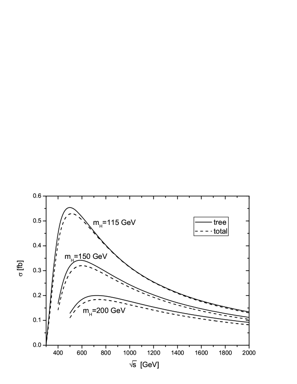
Figure 4: The Born and one-loop level corrected cross sections for the $e^{+}e^{-}\to Z^{0}Z^{0}H^{0}~{}$process as the functions of the $e^{+}e^{-}$ colliding energy $\sqrt{s}$

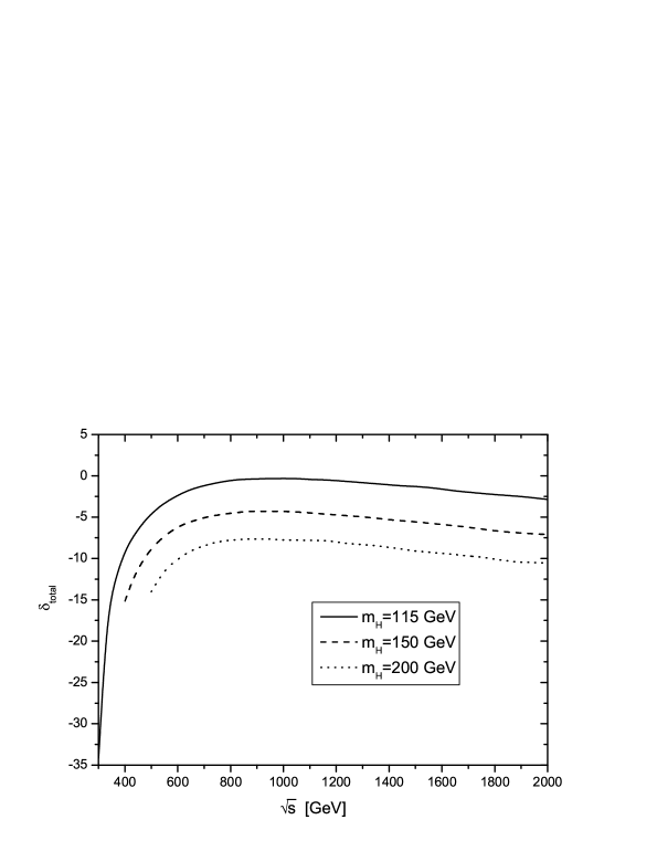
Figure 5: The ${\cal O}(\alpha_{ew})$ relative corrections to the $e^{+}e^{-}\to Z^{0}Z^{0}H^{0}~{}$process as the functions of $\sqrt{s}$

We plot the Born cross section $\sigma_{\rm tree}$ and the electroweak corrected cross section $\sigma_{\rm total}$ as the functions of the Higgs-boson mass $m_{H}$ in Fig.6 with different values of $\sqrt{s}$. It shows that both $\sigma_{\rm tree}$ and $\sigma_{\rm total}$ decrease with the increment of the Higgs-boson mass, and the less the value of $\sqrt{s}$, the more rapidly they drop. We can see in this figure that the cross sections of $\sigma_{\rm tree}$ and $\sigma_{\rm total}$ with $\sqrt{s}=2000~{}{\rm GeV}$ are insensitive to $m_{H}$, and the corresponding curves are stable as the increment of $m_{H}$ from $100~{}GeV$ to $200~{}GeV$. The figure shows also that each curve for the one-loop corrected cross section has two spikes, which just reflect the resonance effects of the virtual corrections at the positions of $m_{H}=2m_{W}$ and $m_{H}=2m_{Z}$, respectively. Since we do not take the complex masses of the $W^{\pm}$ and $Z^{0}$ bosons in the calculation of one-loop integrals, the numerical results in the vicinities of $m_{H}=2m_{W}$ and $m_{H}=2m_{Z}$ are not reliable.

Fig.7 shows the relationship between the full ${\cal O}(\alpha_{ew})$ relative correction of the $e^{+}e^{-}\to Z^{0}Z^{0}H^{0}$ process and the Higgs-boson mass $m_{H}$. We find that the curves for different values of colliding energy decrease with the increment of Higgs-boson mass $m_{H}$. The relative corrections for $\sqrt{s}=500~{}{\rm GeV}$ have negative values, and are generally smaller than the corresponding ones for $\sqrt{s}=800~{}{\rm GeV}$ and $\sqrt{s}=2000~{}{\rm GeV}$. We can see from the figure that on each curve there are also two spikes at the positions of $m_{H}=2m_{W}$ and $m_{H}=2m_{Z}$ due to the resonance effects. Again the numerical relative corrections in those positions are unreliable for the same reason as declared for Fig.6. For $\sqrt{s}=500~{}{\rm GeV}$, the most favorable colliding energy for $e^{+}e^{-}\to Z^{0}Z^{0}H^{0}~{}$process with intermediate Higgs-boson mass, the relative correction decreases from $-3.24\%$ to $-13.8\%$ as $m_{H}$ increases from $100~{}GeV$ to $200~{}GeV$. We can also read out from the figure that when Higgs-boson mass $m_{H}$ increases from $100~{}GeV$ to $200~{}GeV$, the relative correction for $\sqrt{s}=800~{}{\rm GeV}$ goes down from $0.728\%$ to $-7.82\%$, and from $-1.29\%$ to $-11.1\%$ for $\sqrt{s}=2000~{}{\rm GeV}$.

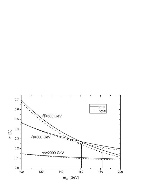
Figure 6: The Born cross section and the one-loop level corrected cross section as the functions of the Higgs-boson mass $m_{H}$

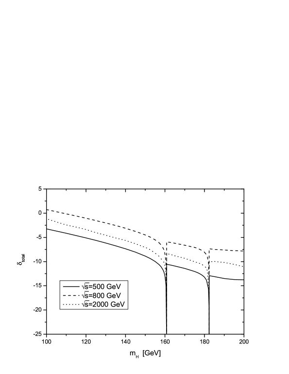
Figure 7: The full ${\cal O}(\alpha_{ew})$ relative corrections to the $e^{+}e^{-}\to Z^{0}Z^{0}H^{0}~{}$process as the functions of the Higgs-boson mass $m_{H}$

In Table 1 we list and compare some numerical results of the radiative corrections to $e^{+}e^{-}\to Z^{0}Z^{0}H^{0}~{}$process contributed by the QED correction part, the weak correction part and the total electroweak one-loop correction. In our calculation we set the soft cutoff $\Delta E/E_{b}$ being $10^{-2}$. From the table we can see that when $\sqrt{s}=500~{}GeV$ and $m_{H}=115,~{}150~{}GeV$, the full QED one-loop corrections have negative signs and are much larger than the weak corrections, while when $\sqrt{s}=1000~{}GeV$ and $m_{H}=115,~{}150~{}GeV$, the weak corrections become important and their absolute values of the weak correction part are comparable with those of the QED correction part. For the case with $\sqrt{s}=1000~{}GeV$ and $m_{H}=115~{}GeV$, the large cancellation between the corrections from the QED and weak parts makes a relative small total one-loop electroweak correction.

$\sqrt{s}$(GeV)	$m_{H}$(GeV)	$\sigma^{QED}_{V+S}(fb)$	$\sigma^{QED}_{hard}(fb)$	$\sigma^{W}(fb)$	$\delta_{total}$(%)	$\delta^{QED}$(%)	$\delta^{W}$(%)
500	115	-0.2587	0.2333	-0.0002	-4.621	-4.576	-0.045
	150	-0.1491	0.1223	-0.0014	-8.857	-8.412	-0.445
1000	115	-0.1538	0.1738	-0.0210	-0.320	6.360	-6.680
	150	-0.1191	0.1293	-0.0207	-4.317	4.204	-8.521

Table 1: The comparison between the numerical results contributed by the QED correction part, the weak correction part and the total electroweak ${\cal O}(\alpha_{ew})$ correction to $e^{+}e^{-}\to Z^{0}Z^{0}H^{0}~{}$process

IV Summary

In this paper we calculate the full ${\cal O}(\alpha_{ew})$ electroweak radiative correction to the $e^{+}e^{-}\to Z^{0}Z^{0}H^{0}$ process within the framework of the SM at linear colliders. We analyze the dependence of the Born cross section, the full ${\cal O}(\alpha_{ew})$ electroweak corrected cross section and the relative correction on colliding energy $\sqrt{s}$ and Higgs-boson mass $m_{H}$. From the numerical results we find that the full ${\cal O}(\alpha_{ew})$ electroweak correction significantly suppresses the Born cross section. When $\sqrt{s}=2000~{}{\rm GeV}$, both the Born and corrected cross sections are insensitive to Higgs-boson mass $m_{H}$. But when $\sqrt{s}$ is relatively smaller, e.g., $\sqrt{s}=500~{}{\rm GeV}$ or $800~{}{\rm GeV}$, both the Born and corrected cross sections decrease sharply with the increment of Higgs-boson mass $m_{H}$. In our chosen parameter space, the relative corrections are in the value range between $1.0\%$ and $-15\%$. These corrections are so remarkable that we must consider them in the precise experimental analysis.

Acknowledgments:

This work was supported in part by the National Natural Science Foundation of China and a special fund sponsored by Chinese Academy of Sciences.

Figure Captions

Figure 1 The tree-level Feynman diagrams for the process $e^{+}e^{-}\to Z^{0}Z^{0}H^{0}~{}$.

Figure 2 The pentagon Feynman diagrams for the process $e^{+}e^{-}\to Z^{0}Z^{0}H^{0}~{}$.

Figure 3 The ${\cal O}(\alpha_{ew})$ relative correction to the $e^{+}e^{-}\to Z^{0}Z^{0}H^{0}~{}$process as a function of the soft cutoff $\Delta E/E_{b}$.

Figure 4 The Born and one-loop level corrected cross sections for the $e^{+}e^{-}\to Z^{0}Z^{0}H^{0}~{}$process as the functions of the $e^{+}e^{-}$ colliding energy $\sqrt{s}$.

Figure 5 The ${\cal O}(\alpha_{ew})$ relative corrections to the $e^{+}e^{-}\to Z^{0}Z^{0}H^{0}~{}$process as the functions of $\sqrt{s}$.

Figure 6 The Born cross section and the one-loop level corrected cross section as the functions of the Higgs-boson mass $m_{H}$.

Figure 7 The full ${\cal O}(\alpha_{ew})$ relative corrections to the $e^{+}e^{-}\to Z^{0}Z^{0}H^{0}~{}$process as the functions of the Higgs-boson mass $m_{H}$.

References

- [1] S. L. Glashow, Nucl. Phys. 22, (1961) 579; S. Weinberg, Phys. Rev. Lett. 1, (1967) 1264; A. Salam, Proc. 8th Nobel Symposium Stockholm 1968, ed. N. Svartholm(Almquist and Wiksells, Stockholm 1968) p.367; H. D. Politzer, Phys. Rep. 14, (1974) 129.
- [2] P. W. Higgs, Phys. Lett. 12, (1964) 132; Phys. Rev. Lett. 13, (1964) 508; Phys. Rev. 145, 1156 (1966); F. Englert and R. Brout, Phys. Rev. Lett. 13, 321 (1964); G. S. Guralnik, C. R. Hagen and T. W. B. Kibble, Phys. Rev. Lett. 13, (1964) 585; T. W. B. Kibble, Phys. Rev. 155, (1967) 1554.
- [3] (ALEPH), (DELPHI), (L3) and (POAL) Collaborations, the LEP working group for Higgs boson searches’LHWG Note 2002-01 (2002), in ICHEP’02 Amsterdam, 2002; and additional updates at http://lephiggs.web.cern.ch/LEPHIGGS/www/Welcome.html; P. A. McNamara and S. L. Wu, Rept. Prog. Phys. 65, (2002) 465.
- [4] The LEP Collaborations: ALEPH Collaboration, DELPHI Collaboration, L3 Collaboration, OPAL Collaboration, the LEP Electroweak Working Group, the SLD Electroweak, Heavy Flavour Groups, CERN-PH-EP/2004-069, LEPEWWG/2004-01, arXiv:hep-ex/0412015.
- [5] The LEP Collaborations, LEPEWWG/TGC/2002-03 (Sept. 2001); ’The QCD/SM Working Group: Summary Report’, hep-ph/0204316.
- [6] K Abe et al., ”Particle physics experiments at JLC”, arXiv:hep-ph/0109166; J.A. Aguilar-Saavedra et al., TESLA Technical Design Report Pert III: Physics at an Linear Collider,” arXiv:hep-ph/0106315; T Abe et al.,” Linear collider physics resource book for Snowmass 2001. 2: Higgs and supersymmetry studies,” in Proc. of the APS/DPF/DPB Summer Study on the Future of Particle Physics(Snowmass 2001) ed. R. Davidon and C. Quigg, arXiv:hep-ex/0106056.
- [7] M.Baillargeon, F. Boudjema, F.Cuypers, E. Gabrielli, and B. Mele, Nucl.Phys. B424 (1994) 343-373.
- [8] S. Dawson and L. Reina, Phys. Rev. D59, 054012 (1999).
- [9] Y. You, W.-G. Ma, H. Chen, R.-Y. Zhang, Y.-B. Sun, H.-S. Hou, Phys.Lett. B571 (2003) 85-91.
- [10] G. Belanger, F. Boudjema, J. Fujimoto, T. Ishikawa, T. Kaneko, K. Kato, Y. Shimizu, Y. Yasui, Phys. Lett. B571(2003)163-172; A.Denner, S.Dittmaier, M.Roth, M.M.Weber, Phys. Lett. B575(2003)290-299.
- [11] J.-J. Liu, W.-G. Ma, L. Han, R.-Y. Zhang, Y. Jiang, P. Wu, Phys. Rev. D72 (2005) 033010
- [12] H. Chen, W.-G. Ma, R.-Y. Zhang, P.-J. Zhou, H.-S. Hou, Y.-B. Sun, Nucl. Phys. B683 (2004) 196-218.
- [13] R.-Y. Zhang, W.-G. Ma, H. Chen, Y.-B. Sun, H.-S. Hou, Phys.Lett. B578 (2004) 349-358.
- [14] G. Belanger, F. Boudjema, J. Fujimoto, T. Ishikawa, T. Kaneko, Y. Kurihara, K. Kato, Y. Shimizu, Phys. Lett. B576(2003) 152-164.
- [15] T. Hahn, Comp. Phys. Commun. 140 (2001) 418.
- [16] T. Hahn, M. Perez-Victoria, Comput. Phys. Commun. 118 (1999) 153, arXiv:hep-ph/9807565; T. Hahn, MPP-2004-71, arXiv:hep-ph/0406288.
- [17] G.J. van Oldenborgh, Comput. Phys. Commun 58(1991)1.
- [18] A. Denner and S. Dittmaier, Nucl. Phys. B658(2003) 175.
- [19] S. Eidelman, et al., Phys. Lett. B592 (2004) 1.
- [20] G. ’t Hooft and M. Veltman, Nucl. Phys. B44, (1972) 189.
- [21] D. A. Ross and J. C. Taylor, Nucl. Phys. B51, (1979) 25.
- [22] A. Denner, Fortschr. Phys. 41, (1993) 307.
- [23] G. Passarino and M. Veltman, Nucl. Phys. B160, (1979) 151.
- [24] A. Denner and S. Dittmaier, Nucl. Phys. B658, (2003) 175.
- [25] W. T. Giele and E. W. N. Glover, Phys. Rev. D46, (1992) 1980; W. T. Giele, E. W. Glover and D. A. Kosower, Nucl. Phys. B403, (1993) 633.
- [26] G. ’t Hooft and Veltman, Nucl. Phys. B153, (1979) 365.
- [27] F. Jegerlehner, Report No. DESY 01-029 (unpublished).