We investigate lepton flavor violation in the context of intersecting D-brane models. We point out that these models have a source to generate flavor violation in the trilinear scalar couplings while the geometry of the construction leads to degenerate soft scalar masses for different generations (as in the minimal supergravity model) at the string scale. The trilinear scalar couplings are not proportional to the Yukawa couplings when the $F$-term of the $U$-moduli contribution is non-zero. Consequently, the lepton flavor violating decay processes are generated. Only other sources of flavor violations in this model are the Dirac neutrino Yukawa coupling and the Majorana couplings. The observed fermion mixings are realized from the “almost rank 1” Yukawa matrices, which generate a simple texture for the trilinear scalar terms. We calculate the branching ratios of $\tau\rightarrow\mu\gamma$, $\mu\rightarrow e\gamma$ and the electric dipole moment of the electron in this model. We find that the observation of all the lepton flavor violating decay processes and the electric dipole moment will be able to sort out different flavor violating sources.

1 Introduction

The standard model is well established to describe physics below the weak scale while it also has a number of parameters, especially in the flavor sector. Indeed, the patterns of masses and mixings for quarks and leptons are not very simple and should be explained in a fundamental way. Thus, one expects that there exists more fundamental physics beyond the standard model and the masses and the mixings are described by some fundamental parameters.

Supersymmetry (SUSY) is the most promising candidate of new physics. SUSY models can explain gauge hierarchy problems and suggest gauge unification such as $SU(5)$ grand unified theory (GUT) with successful gauge coupling unification in the minimal extension of the SUSY standard model (MSSM). However, SUSY does not solve flavor puzzles, Rather, it increases the number of parameters with flavor indices to more than hundred in general. Nevertheless, people are not discouraged to consider SUSY models since the SUSY breaking parameters with flavor indices are constrained to suppress flavor changing neutral currents (FCNC) [1]. Actually, one expects that the FCNC suppression may be realized by a flavor symmetry, which may give us a hint of the fundamental physics for flavors.

The minimality of the SUSY breaking parameters is assumed in the minimal supergravity (mSUGRA) mediated SUSY breaking scenario [2]: SUSY breaking scalar masses are universal and the scalar trilinear couplings ($A$-terms) are proportional to the Yukawa couplings. The degeneracy of the SUSY breaking masses corresponds to the $U(3)_{L}\times U(3)_{R}$ flavor symmetry. On the other hand, it is hard to relate the proportionality of $A$-terms to such flavor symmetries since the Yukawa couplings themselves break the symmetries.

The fundamental questions for the flavor sector are the following: 1) Why do fermions replicate with different masses? 2) Can we explain the pattern of the masses and the mixings for quarks and leptons? 3) Why does the flavor symmetry seem unbroken in the SUSY breaking mass terms, while the fermion masses break the flavor symmetry? 4) Is the $A$-term proportionality feasible? When is this proportionality feasible? How does it look like if it is not proportional?

The intersecting D-brane models [3, 4, 5] may answer such questions. The string theory can describe the particle field theory as an effective theory, and thus, in principle, it has a potential to calculate all the parameters by using a few fundamental parameters. Indeed, the intersecting D-branes are interesting approaches to construct the standard model. The $N$ stack of D-branes can form $U(N)$ gauge fields as zero modes of open strings attaching on the D-branes. Open strings can be attached at the intersection between the $N$ stack and the $M$ stack of D-branes, and massless chiral fermions belonging to $(N,\bar{M})$ bi-fundamental representation can appear. Such a situation is very attractive to obtain quark and lepton fields not only in the standard model [6] but also in the unified models [7, 8]. When the extra dimensions are compactified by torus such as $T^{6}=T^{2}\times T^{2}\times T^{2}$, the intersecting point of the D-branes can be multiplicated, and thus the fermions are replicated. The number of generation is therefore a topological number.

In addition to the realization of the standard-like models, the effective supergravity Lagrangian is calculable [9, 10, 11, 12]. The Yukawa coupling is obtained as an open string scattering for the triangle formed by the D-branes. The couplings are described as $e^{-kA}$, where the triangle area $A$ is formed by three intersecting points. For the toroidal compactification models, the Yukawa couplings are written as theta function of geometrical parameters including instanton effects. In simple models, the Yukawa matrices are written in the factorized form $y_{ij}=x^{L}_{i}x^{R}_{j}$ [9, 13]. This originates from a geometrical reason that the left- and the right-handed fermions are replicated at the intersecting points on different tori, and the Yukawa couplings are given as an exponential form of sum of the triangle areas. As a result of the factorized form of the Yukawa coupling, the Yukawa matrices are rank 1, and thus only the 3rd generation fermions are massive. In order to construct a realistic model, this issue of Yukawa matrices needs to be resolved and several possibilities have been considered [13, 14]. The Yukawa matrices can be hierarchical when the Yukawa matrices are “almost rank 1” by including higher order effects or quantum corrections. The exponential suppression of the Yukawa coupling is also available to obtain hierarchical masses. In Ref.[14], we have discussed that the observed patterns of fermion mixings can be easily reproduced if the Yukawa matrices are almost rank 1.

The Kähler metrics of the zero modes can also be calculated as string scattering amplitudes [10] in terms of the moduli fields: dilaton $S$, Kähler moduli $T$, and complex structure moduli $U$. The Kähler metrics are diagonal for the zero modes, and the metrics for the bifundamental fields are determined by the brane configuration parameters such as the relative angles of the D-branes. Since the relative angles are common when the fermions are replicated at the intersection of the D-branes, the Kähler metrics are flavor invisible. Consequently, the SUSY breaking scalar masses are same for different generations. So, the flavor symmetry of the scalar masses can originate from the brane geometry.

When the Kähler metrics remain same for each generation, the Kähler connection parts (which are the derivatives of Kähler metric) of $A$-terms are common. Thus, the non-proportional part of the $A$-term is only the derivative of the Yukawa coupling. The Yukawa couplings which are given as theta functions depend only on the $U$-moduli [12], neither on the $S$ nor the $T$-moduli. As a result, the trilinear scalar couplings are proportional to the Yukawa coupling when the $F$ component of the $U$-moduli is zero. If $F^{U}\neq 0$, the non-proportional part of $A$-term is acquired, which is proportional to the derivative of the Yukawa matrices.

In this paper, we emphasize the degeneracy of the SUSY breaking mass terms and the $U$-moduli contribution of the trilinear scalar couplings. These contributions are related to the flavor violation and we will study the lepton flavor violation (LFV) processes since the flavor violation in the lepton sector produce much more stringent constraint rather than in the quark sector. The LFV processes, such as $\mu\rightarrow e\gamma$, $\tau\rightarrow\mu\gamma$ and $\tau\rightarrow e\gamma$, are not yet observed, but we have bounds on the branching ratios of these decay modes [15]. The observation of these decay modes would provide information of flavor violation in new physics. It is pointed out that the processes are accessible for SUSY models [16]. In the mainstream of theoretical calculations, the flavor violation in the SUSY breaking parameters is assumed to be absent at the cutoff scale in the mSUGRA. The source of flavor violation originates from the Yukawa couplings such as the Dirac neutrino and the Majorana couplings. The SUSY breaking parameters at the weak scale can acquire flavor violation through renormalization group equations (RGE). Indeed, the off-diagonal elements of the left- and right-handed slepton mass matrices are generated, and the slepton-gaugino loop diagram provides the LFV processes. In the intersecting D-brane models, the flavor degeneracy of the slepton masses at the cutoff scale is realized naturally and the $U$-moduli contribution of $A$-terms can be one of the major sources of flavor violation. We will calculate the branching ratios of different LFV decays and the electric dipole moment (EDM) of the electron, and study whether we can learn the origins of flavor violation from the forthcoming experiments.

This paper is organized as follows: In section 2, we will study the low energy effective action of the zero modes for matter fields in intersecting D-brane models. In section 3, the realization of neutrino mixing angles are obtained in the context of “almost rank 1 Yukawa matrix”. In section 4, we investigate the sources of LFV. In section 5, we will calculate branching ratios of the LFV decays and the EDM of the electron, and compare the results with different setups of flavor violation. Section 6 is devoted to conclusions and discussions.

2 Effective action in the intersecting D-brane models

Our purpose is to deal with the flavor physics and study its phenomenological implications in the intersecting D-brane models. We will consider models with intersecting D6-branes in the type IIA theory [5], which may be equivalent to the models with magnetized D9-branes and D5-branes in the type IIB theory. One can also apply our work to the D7-branes in the type IIB theory in which supersymmetry breaking soft terms can arise from 3-form fluxes [12]. In this section, we will explore the flavor sector of the models without concentrating on the details of any individual model.

The MSSM-like models can be constructed easily by introducing three sets of intersecting D-branes. For example, in the type IIA orientifold models with $T^{6}/Z_{2}\times Z_{2}$ and with the intersecting D6-branes, the $N$ stack of D-branes can form $SU(N/2)$ gauge fields. Massless chiral fermions belong to the $(N/2,\bar{M}/2)$ bi-fundamental representation can appear at the intersection between the $N$ stack and the $M$ stack of D-branes. So, introducing $a,b,c$ branes for $U(4)_{c}$, $U(2)_{L}$ and $U(2)_{R}$ respectively, we can obtain Pati-Salam-like model [17] with quark and lepton fields [8]. The $SU(4)_{c}$ and $SU(2)_{R}$ symmetries are broken to $SU(4)_{c}\rightarrow SU(3)_{c}\times U(1)_{B-L}$ and $SU(2)_{R}\rightarrow U(1)_{R}$ by brane splitting [18], and $U(1)_{B-L}\times U(1)_{R}$ is broken down to $U(1)_{Y}$ by the Higgs mechanism. When the branes are parallel to the orientifolds, the $USp$ gauge symmetry arises. The $SU(2)$ gauge symmetry in the standard model can originate from the $USp$ brane. In order to eliminate the RR tadpole, extra branes are often needed and they may form hidden sectors [19].

Since the extra dimensions are compactified to $T^{6}=T^{2}\times T^{2}\times T^{2}$, the D-branes intersects multiple times and the generations of the fermions are replicated. The intersection numbers $I_{ab}$ for $D_{a}$ and $D_{b}$ branes are topological invariant and can be given by the wrapping numbers and the total magnetic fluxes $(n_{a}^{r},m_{a}^{r})$,

$$I_{ab}=\prod_{r=1}^{3}(n_{a}^{r}m_{b}^{r}-m_{a}^{r}n_{b}^{r}),$$ (1)

where $r$ represents index of each torus. In a simple choice to obtain three generations, the left-handed matter $\Psi^{ab}$ and the right-handed matter $\Psi^{ca}$ are often replicated on different tori.

The important implication of the family replication is that the Kähler metric is flavor diagonal:

$$K=\hat{K}(M,\bar{M})+K_{ab}(M,\bar{M})\Psi_{i}^{ab}\bar{\Psi}_{i}^{ab}+K_{ca}(M,\bar{M})\Psi_{i}^{ca}\bar{\Psi}_{i}^{ca}+\dots,$$ (2)

where $M$ stands for the $S$, $T$ and $U$ moduli and the index $i$ is for the flavor index. In addition to the flavor diagonal nature, the Kähler metric for $\Psi^{ab}$ does not depend on flavor indices for $I_{ab}=I_{ca}=3$. The Kähler metric $K_{ab}(M,\bar{M})$ is determined by the relative angles $\theta_{ab}^{r}$ of the D-branes [10, 11, 12]:

$$K_{ab}\propto e^{\phi_{4}}\prod_{r}(U_{r}+\bar{U}_{r})^{-\nu_{r}}\sqrt{\frac{\Gamma(1-\nu_{r})}{\Gamma(\nu_{r})}}\,.$$ (3)

where $\phi_{4}$ is a 4-dimensional dilaton and $\nu_{r}=\theta_{ab}/\pi$, which are functions of $S$ and $T$ moduli. The moduli dependence of the Kähler metric is determined by the geometrical parameters, and thus the metric is flavor invisible. Therefore, the SUSY breaking scalar mass for the left-handed matter is given below [20] and it has the flavor degeneracy:

$$m^{2}_{ab}=m_{3/2}^{2}+V_{0}-\sum_{M,N}\bar{F}^{\bar{M}}F^{N}\partial_{\bar{M}}\partial_{N}\log K_{ab}\,,$$ (4)

where $m_{3/2}$ is a gravitino mass and $V_{0}$ is the vacuum expectation value of the scalar potential. The scalar mass squared $m_{ca}^{2}$ for the right-handed matter can be similarly written and can also have the flavor degeneracy. Since the relative angles for $ab$ and $ca$ can be different, the scalar masses are not necessarily universal for different representations of matter. We note that the flavor degeneracy can be broken when 2+1 decomposition of the generation is considered, for example, $I_{ab}=2$ and $I_{ab^{\prime}}=1$, where $b^{\prime}$ is a orientifold reflection of the brane $b$. We will choose $I_{ab}=I_{ca}=3$ from now on and there is a $U(3)_{L}\times U(3)_{R}$ flavor symmetry in the SUSY breaking scalar mass terms at the string scale. We emphasize that such a mSUGRA-type flavor structure can be obtained by a geometrical setup of the D-branes.

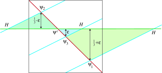
Figure 1: A sketch of brane intersections on a torus.

The Yukawa coupling $\Psi^{ab}\Psi^{bc}\Psi^{ca}$ is induced by the three-point open string scattering. When the left-handed matter $\Psi^{ab}$ and the right-handed matter $\Psi^{ca}$ are replicated in different tori, the Yukawa coupling is factorized:

$$Y_{ij}=x_{i}^{L}(U_{1})x_{j}^{R}(U_{2}).$$ (5)

The $x_{i}^{L,R}$ can be written by theta function [9] with some geometrical parameters such as $\varepsilon$ shown in the Fig.1. Naively, these are given by $e^{-kA}$ where $A$ is the area of the triangle formed by the branes. The Yukawa couplings do not depend on the $S$ and $T$ moduli but depend on the complex structure moduli $U$.

When the Yukawa coupling is factorized, the matrix is rank 1 and consequently $U(2)_{L}\times U(2)_{R}$ flavor symmetry remains and the fermions of 1st and 2nd generation are massless. Surely such a situation is not viable, and there exists several discussion on this issue [13]. For example, we have suggested that the multi-point function of the string scattering including extra branes can increase the rank of the Yukawa matrix [14]. In this paper, we do not specify how to increase the rank, but we assume the factorizability of the Yukawa coupling at the leading order since this assumption leads to interesting phenomenological implications which we will see in the next section.

The scalar trilinear coupling ($A$-term) is given as [20]

$$A_{ij}=F^{M}\left[\left(\hat{K}_{M}-\partial_{M}\log(K_{ab}K_{bc}K_{ca})\right)Y_{ij}+\partial_{M}Y_{ij}\right],$$ (6)

and the coupling is proportional to the Yukawa coupling if $F^{U}=0$. However, when $F^{U}\neq 0$, the flavor violation is generated,

$$F^{U_{r}}\partial_{U_{r}}Y_{ij}=F^{U_{1}}\dot{x}_{i}^{L}x_{j}^{R}+F^{U_{2}}x_{i}^{L}\dot{x}_{j}^{R},$$ (7)

where $\dot{x}$ stands for the derivative by the $U$ moduli. The $U$ moduli contribution in the $A$-term can be the source of flavor violation. In this paper, we will emphasize the effect of the $U$ moduli contribution.

3 Application of “almost rank 1 Yukawa matrices”

We will first discuss the mixing angles for neutrino oscillation in the context of “almost rank 1 Yukawa matrix” [14].

The Yukawa matrix for the charged-leptons is given as $Y_{e}=Y_{0}+\delta Y$ where $Y_{0}$ is the rank 1 matrix, and $\delta Y$ is a small correction to generate electron and muon masses. The rank 1 matrix can be expressed as

$$Y_{0}=\left(\begin{array}[]{c}c_{1}\\ b_{1}\\ a_{1}\end{array}\right)\left(\begin{array}[]{ccc}c_{2}&b_{2}&a_{2}\end{array}\right)=\left(\begin{array}[]{ccc}c_{1}c_{2}&c_{1}b_{2}&c_{1}a_{2}\\ b_{1}c_{2}&b_{1}b_{2}&b_{1}a_{2}\\ a_{1}c_{2}&a_{1}b_{2}&a_{1}a_{2}\end{array}\right),$$ (8)

and $a_{i},b_{i},c_{i}$ can be given by theta function [9]. Note that $a_{i},b_{i},c_{i}$ can be rotated to be real by field redefinitions.

Now let us work in a basis where the mass matrix of the light neutrino is diagonalized. Then the diagonalizing matrix of $Y_{e}$ is the MNSP (Maki-Nakagawa-Sakata-Pontecorvo) matrix: $U_{\rm MNSP}=U_{L}^{e*}$, where $U_{L}^{e}Y_{e}U_{R}^{e\dagger}=Y_{e}^{\rm diag}$. The $3\times 3$ unitary diagonalization matrix has three mixing angles, and those angles may be generically large since $a_{i},b_{i},c_{i}$ are all order one parameters. However, one of the three mixing angles of $U_{L(R)}$ is unphysical in the limit $\delta Y\rightarrow 0$ since 1st and 2nd generation masses are equal to be zero and the $U(2)_{L}\times U(2)_{R}$ flavor symmetry remains unbroken. The small correction, $\delta Y$, eliminates the degeneracy and the mixing angle of $U_{L(R)}$ is fixed. Namely, the two mixing angles in $U_{L(R)}$ are generically large and one mixing angle is determined by a small correction $\delta Y$. For example, when the small correction is $\delta Y={\rm diag}(0,0,\epsilon)$, the Yukawa coupling becomes rank 2 and the eigenvector for the zero eigenvalues is $\propto(b_{1},-c_{1},0)$ for $U_{L}$. As a result, one can find that $U_{e3}(=\sin\theta_{13})$ is exactly zero in this example. The small correction needs to be more realistic to generate the electron mass, and then $U_{e3}$ can acquire a small non-zero value. Consequently, the two large mixings for solar and atmospheric neutrinos and the small mixing for $\theta_{13}$ is elegantly realized in this scheme.

The approximate diagonalization matrix $U_{L}^{0}$ is given as

$$U_{L}^{0}=\left(\begin{array}[]{ccc}\cos\theta^{L}_{s}&-\sin\theta^{L}_{s}&0\\ \cos\theta^{L}_{a}\sin\theta^{L}_{s}&\cos\theta^{L}_{a}\cos\theta^{L}_{s}&-\sin\theta^{L}_{a}\\ \sin\theta^{L}_{a}\sin\theta^{L}_{s}&\sin\theta^{L}_{a}\cos\theta^{L}_{s}&\cos\theta^{L}_{a}\end{array}\right),$$ (9)

where $\tan\theta_{s}^{L}=c_{1}/b_{1}$ and $\tan\theta_{a}^{L}=\sqrt{b_{1}^{2}+c_{1}^{2}}/a_{1}$. The right-handed $U_{R}^{0}$ can be also described similarly. Then the MNSP matrix can be written as

$$U_{\rm MNSP}=V^{e*}_{L}U_{L}^{0}\,,$$ (10)

where $V_{L}^{e}$ is a diagonalizing matrix of $U_{L}^{0}Y_{e}U_{R}^{0\rm T}=Y_{0}^{\rm daig}+U_{L}^{0}\delta YU_{R}^{0\rm T}$.

In the quark sector, the CKM (Cabibbo-Kobayashi-Maskawa) matrix is written as $V_{\rm CKM}=U^{u}_{L}U^{d\dagger}_{L}$, where the unitary matrices are $U^{u,d}_{L}Y_{u,d}U^{u,d\dagger}_{R}=Y_{u,d}^{\rm diag}$. The Yukawa matrices are given as $Y^{u,d}_{ij}=x_{i}^{L}x_{j}^{R(u,d)}+\delta Y^{u,d}_{ij}$. In a similar way in the charged lepton sector, the unitary matrices can be written in the form $U^{u,d}_{L}=V_{L}^{u,d}U_{L}^{0}$. Since the left-hand part $x_{i}^{L}$ is common for both up- and down-type quarks, the large mixings in $U^{u,d}_{L}$ get cancelled, and the CKM mixings are small: $V_{\rm CKM}=V^{u}_{L}V^{d\dagger}_{L}$. Since the up-type quarks are more hierarchical than the down-type quarks, the CKM matrix is expected to be $V_{\rm CKM}\simeq V_{L}^{d\dagger}$. If we have quark-lepton unification, we have a relation $V_{L}^{d}\simeq V_{L}^{e}$. Then the MNSP matrix is

$$U_{\rm MNSP}\simeq V_{\rm CKM}^{\rm T}U_{L}^{0}.$$ (11)

This type of MNSP matrix is surveyed as an ansatz in Ref.[21].

Once the MNSP matrix is given in the form Eq.(10), we obtain the mixing angles for neutrino oscillation as follows [14]:

$$\sin\theta_{13}\simeq\sin\theta_{a}^{L}\sin\theta_{12}^{e},\quad\theta_{\rm atm}\simeq\theta_{a}^{L},\quad\theta_{\rm sol}\simeq\theta_{s}^{L}\pm\theta_{13}\cot\theta_{\rm atm}\cos\delta_{\rm MNSP}\,,$$ (12)

where $\theta_{12}^{e}$ is a mixing angle in $V_{L}^{e}$, and $\theta_{13}^{e}$ and $\theta_{23}^{e}$ are neglected since they are expected to be small as in the quark sector. The atmospheric neutrino mixing is almost maximal and the solar mixing angle is large but not maximal since $c_{1}\mathrel{\mathchoice{\lower 2.58334pt\vbox{\halign{$\m@th\displaystyle\hfil#\hfil$\cr<\crcr\sim\crcr}}}{\lower 2.58334pt\vbox{\halign{$\m@th\textstyle\hfil#\hfil$\cr<\crcr\sim\crcr}}}{\lower 2.58334pt\vbox{\halign{$\m@th\scriptstyle\hfil#\hfil$\cr<\crcr\sim\crcr}}}{\lower 2.58334pt\vbox{\halign{$\m@th\scriptscriptstyle\hfil#\hfil$\cr<\crcr\sim\crcr}}}}b_{1}\mathrel{\mathchoice{\lower 2.58334pt\vbox{\halign{$\m@th\displaystyle\hfil#\hfil$\cr<\crcr\sim\crcr}}}{\lower 2.58334pt\vbox{\halign{$\m@th\textstyle\hfil#\hfil$\cr<\crcr\sim\crcr}}}{\lower 2.58334pt\vbox{\halign{$\m@th\scriptstyle\hfil#\hfil$\cr<\crcr\sim\crcr}}}{\lower 2.58334pt\vbox{\halign{$\m@th\scriptscriptstyle\hfil#\hfil$\cr<\crcr\sim\crcr}}}}a_{1}$ and $\tan\theta_{a}^{L}=\sqrt{b_{1}^{2}+c_{1}^{2}}/a_{1}$, $\tan\theta_{s}^{L}=c_{1}/b_{1}$.

The smallness of the neutrino masses are explained by the seesaw mechanism [22]. We note that the large mixing angles between the charged-lepton and the neutrino Dirac Yukawa coupling can also get cancelled as in the quark sector. Thus, the favorable situation is when the $SU(2)_{L}$ triplet Majorana part is dominant in the type II seesaw [23]

$$m_{\nu}^{\rm light}=M_{L}-M_{\nu}^{D}M_{R}^{-1}M_{\nu}^{D\rm T}.$$ (13)

The Majorana couplings for both left- and right-handed leptons

$$\frac{1}{2}f_{L}\ell\ell\Delta_{L}+\frac{1}{2}(f_{R}^{ee}e^{c}e^{c}\Delta_{R}^{--}+f_{R}^{\nu\nu}\nu^{c}\nu^{c}\Delta_{R}^{0}+\sqrt{2}f_{R}^{\nu e}\nu^{c}e^{c}\Delta_{R}^{-}),$$ (14)

can be generated by multi-point functions in each torus [14].

4 Possible sources of lepton flavor violation

In this section, we will describe the sources of the LFV processes such as $\mu\rightarrow e\gamma$ and $\tau\rightarrow\mu\gamma$.

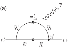
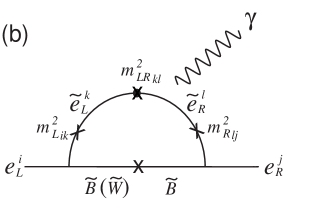
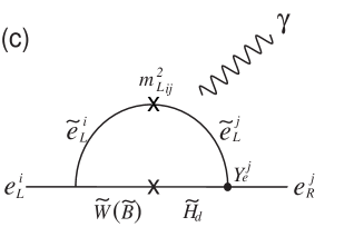
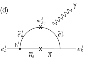
Figure 2: Chargino (a) and neutralino (b,c,d) loop diagrams to generate the LFV processes. The off-diagonal elements of $m^{2}_{L}$ and $m^{2}_{R}$ come from $m^{2}_{\tilde{\ell}}$ and $m^{2}_{\tilde{e}}$, respectively. The mark $\bullet$ stands for a chirality flipping. The chirality flipping for Bino diagram (b) is given as $m^{2}_{LR}=A_{e}v_{d}-\mu\tan\beta\,M_{e}$. There are diagrams in which the chirality is flipped in the external lines, but contributions from such diagrams are small.

In SUSY models, the LFV processes are described by loop diagrams. The charginos and neutralinos propagate in the loop as shown in the Fig.2. When the SUSY breaking mass terms and the $A$-terms violate lepton flavor, the branching ratio of the LFV processes can be comparable to the experimental results. So the flavor structure of the SUSY breaking parameters is constrained [1].

When the SUSY breaking masses are universal and the $A$-term coefficient is proportional to the Yukawa coupling, there is no source for any LFV. However, even if there exists no LFV source in the SUSY breaking parameters at the cutoff scale, the sources for LFV can be generated through the neutrino Dirac Yukawa couplings as long as the coupling matrices are not proportional to the charged lepton Yukawa matrix. The Majorana couplings can also generate LFV.

The RGEs above the scale of right-handed neutrino Majorana masses and and triplet Higgs fields are written in a proper notation as

$$(4\pi)^{2}\frac{d}{d\ln Q}m_{\tilde{\ell}}^{2} \!\!= \!\!\{Y_{e}Y_{e}^{\dagger},m_{\tilde{\ell}}^{2}\}+\{Y_{\nu}Y_{\nu}^{\dagger},m_{\tilde{\ell}}^{2}\}+3\{f_{L}f_{L}^{\dagger},m_{\tilde{\ell}}^{2}\}$$

$$\!\!+ \!\!2(Y_{e}m_{\tilde{e}}^{2}Y_{e}^{\dagger}+m_{H_{d}}^{2}Y_{e}Y_{e}^{\dagger}+A_{e}A_{e}^{\dagger})+2(Y_{\nu}m_{\tilde{\nu}}^{2}Y_{\nu}^{\dagger}+m_{H_{u}}^{2}Y_{\nu}Y_{\nu}^{\dagger}+A_{\nu}A_{\nu}^{\dagger})$$

$$\!\!+ \!\!6(f_{L}(m_{\tilde{\ell}}^{2})^{\rm T}f_{L}^{\dagger}+f_{L}f_{L}^{\dagger}m_{\Delta_{L}}^{2}+A_{f_{L}}A_{f_{L}}^{\dagger})$$

$$\!\!- \!\!8(\frac{1}{4}g^{\prime 2}M_{1}^{2}+\frac{3}{4}g_{2}^{2}M^{2}_{2})-g^{\prime 2}S\,,$$

$$(4\pi)^{2}\frac{d}{d\ln Q}m_{\tilde{e}}^{2} \!\!= \!\!2\{Y_{e}^{\dagger}Y_{e},m_{\tilde{e}}^{2}\}+\{f_{R}^{ee\dagger}f_{R}^{ee},m_{\tilde{e}}^{2}\}+2\{f_{R}^{\nu e\dagger}f_{R}^{\nu e},m_{\tilde{e}}^{2}\}$$

$$\!\!+ \!\!4(Y_{e}^{\dagger}m_{\tilde{\ell}}^{2}Y_{e}+m_{H_{d}}^{2}Y_{e}^{\dagger}Y_{e}+A_{e}^{\dagger}A_{e})$$

$$\!\!+ \!\!2(f_{R}^{ee\dagger}(m_{\tilde{e}}^{2})^{\rm T}f_{R}^{ee}+f_{R}^{ee\dagger}f_{R}^{ee}m_{\Delta_{R}^{--}}^{2}+A_{f_{R}}^{ee\dagger}A_{f_{R}}^{ee})$$

$$\!\!+ \!\!4(f_{R}^{\nu e\dagger}(m_{\tilde{\nu}}^{2})^{\rm T}f_{R}^{\nu e}+f_{R}^{\nu e\dagger}f_{R}^{\nu e}m_{\Delta_{R}^{-}}^{2}+A_{f_{R}}^{\nu e\dagger}A_{f_{R}}^{\nu e})$$

$$\!\!- \!\!8g^{\prime 2}M_{1}^{2}+2g^{\prime 2}S\,,$$

where $\{X,Y\}=XY+YX$ and $S$ is a trace of SUSY breaking masses with hypercharge weight.

As it has been emphasized, the SUSY breaking scalar masses are universal due to the geometrical setup. On the other hand, if the $F$-terms of $U$-moduli are zero, the $A$-terms are proportional to the Yukawa couplings. However, the non-zero values of $F^{U}$ provide a source of LFV in the form as shown in the Eq.(7). Let us see the $U$-moduli contribution in the basis where the charged lepton Yukawa matrix is diagonal: $U_{L}^{e}Y_{e}U_{R}^{e\rm T}=Y_{e}^{\rm diag}$. Since $U_{L}^{0}x^{L}=(0,0,\sqrt{a_{1}^{2}+b_{1}^{2}+c_{1}^{2}})^{\rm T}$, the derivative of the rank 1 part $(Y_{0})_{ij}=x^{L}_{i}x^{R}_{j}$ is written as

$$U_{L}^{e}(\partial_{U}Y_{0})U_{R}^{e\dagger}=V_{L}^{e}\left(\begin{array}[]{ccc}0&0&{\tt x}\\ 0&0&{\tt x}\\ {\tt x}&{\tt x}&{\tt x}\end{array}\right)V_{R}^{e\dagger}\,,$$ (17)

where the non-zero values in the entries are shown by $\tt x$. Note that the (1,3) and (3,1) elements in the above matrix become zero when $\tan\theta_{s}^{L,R}=1$. Since the mixing angles in $V^{e}_{L,R}$ are small, the elements $A_{ij}$ $(i,j\leq 2)$ can be small while the elements $A_{i3}$ and $A_{3i}$ can be large. In fact, the experimental bounds ${\rm Br}(\mu\rightarrow e\gamma)<1.2\times 10^{-11}$ [15] and the EDM of the electron $|d_{e}|<1.6\times 10^{-27}$ [24] provide the most severe constraint on $A_{12}$ and Im$A_{11}$. Due to the structure of Eq.(17), $A_{i3}$ and $A_{3i}$ from the $U$ moduli contribution can be the sources of LFV while keeping the elements $A_{12}$ and $A_{11}$ to be small. The $U$-moduli contribution can generate the off-diagonal elements of SUSY breaking scalar mass squared matrices through the RGEs.

In the minimal SUGRA, the non-proportionality of the $A$-term never develops. In the intersecting D-brane models, the non-minimality of the $A$-terms can be included when $F^{U}\neq 0$ while the SUSY breaking scalar masses have degeneracy for different generations at the cutoff scale due to the geometrical setup of D-branes. Due to the particular form of the $U$-moduli contribution as shown in the Eq.(17), the (1,3) element can be larger than the usual hierarchical assumptions for the non-minimal $A$-terms. The RGE effects are not decoupled till the electroweak scale and due to this the off-diagonal elements for both left- and right-handed slepton mass matrices are generated. The right-handed off-diagonal elements are always larger than the left-handed elements due to a difference in the coefficients of the terms involving $A_{e}$s in the RGEs.

We enumerate the sources of LFV in the SUSY breaking scalar mass matrices at the weak scale in the mSUGRA model as follows:

1. Neutrino Dirac Yukawa coupling [16]

   The neutrino Dirac Yukawa coupling $Y_{\nu}$ can generate the off-diagonal elements of left-handed SUSY breaking slepton mass matrix $m^{2}_{\tilde{\ell}}\,$. Hence, the chargino contribution can dominate in the LFV processes. The RGE effects are decoupled at the right-handed neutrino Majorana mass scale.

2. Majorana coupling for left- and right-handed leptons

   The left-handed Majorana coupling $f_{L}$ is needed in type II seesaw. The right-handed Majorana coupling $f_{R}$ also participates in the light neutrino mass when $B-L$ charge is gauged. The Majorana coupling $f_{L}$ and $f_{R}$ can generate the off-diagonal elements of both left- and right-handed slepton mass matrices, $m^{2}_{\tilde{\ell}}$, $m^{2}_{\tilde{e}}$. The RGE effects are decoupled at the $\Delta_{L,R}$ mass scale, and the right-handed neutrino Majorana mass scale for $f_{R}^{\nu e}$ coupling.

3. SU(5) GUT [25] or the left-right unification [26]

   Since the right-handed selectron can be unified in the $\bf 10$ dimensional representation of the $SU(5)$ grand unification, the off-diagonal elements of right-handed selectron can be generated above the unified scale. The generated off-diagonal elements of $m_{\tilde{e}}^{2}$ are related to the CKM mixings. In the left-right unified models, the two Higgs bidoublets are needed to generate the CKM mixings, and the two different Yukawa matrices are sources of off-diagonal elements for both left- and right-handed sleptons. We do not discuss these sources in this paper.

5 Numerical studies

In this section, we will show the numerical calculations of the branching ratio of the LFV decays and the EDM of the electron in the context of intersecting D-brane models.

We set up the parameters to show the numerical results as follows. The charged lepton mass matrix is given as rank 1 matrix plus small correction. The rank 1 matrix is given as Eq.(8) in the basis where light neutrino mass matrix is diagonal. In the minimal brane configuration, such as shown in the Fig.1, the parameters are given [14]

$$a_{1}:b_{1}:c_{1}=\vartheta\left[\begin{array}[]{cc}\varepsilon\\ 0\end{array}\right](t):\vartheta\left[\begin{array}[]{cc}-\frac{1}{3}+\varepsilon\\ 0\end{array}\right](t):\vartheta\left[\begin{array}[]{cc}\frac{1}{3}+\varepsilon\\ 0\end{array}\right](t)\,.$$ (18)

For the calculation, we use $\varepsilon=0.1$ and $t=1.5$. Then $\theta^{L}_{a}=47^{\rm o}$ and $\theta^{L}_{s}=37^{\rm o}$. For simplicity, the Yukawa matrix is assumed to be symmetric. Then $U$-moduli contribution of the $A$-term which is proportional to the derivative of Yukawa coupling is calculated in the basis where the charged lepton Yukawa matrix is diagonal

$$A_{e}^{U}=c\,A_{0}\ V_{L}^{e}\left(\begin{array}[]{ccc}0&0&0.22\\ 0&0&0.26\\ 0.22&0.26&0.84\end{array}\right)V_{R}^{e\dagger}\,,$$ (19)

where $A_{0}$ is a dimensionful coupling coefficient and $c$ is a coefficient. If $F^{U}=0$, $c=0$, the trilinear coupling is given as $A_{e}=A_{0}Y_{e}+A_{e}^{U}$. More precisely, the $U$-moduli derivative of the correction matrix $\delta Y$ may also contribute, but we neglect its contribution here since its $U$-moduli derivative does not appear to be large and has a model dependence. We will choose the mixing angles in $V_{L}^{e}=V_{R}^{e}$ as $\theta_{12}^{e}=0.1$, $\theta_{23}^{e}=0.05$ and $\theta_{13}^{e}=0.005$. There can be 5 phases in the unitary matrix $V_{L}^{e}$ up to an overall phase in general, but for simplicity, we assume that there is no CP phase in $V_{L}^{e}$. The neutrino mixing angles are given in the Eq.(12). In the choice above, $U_{e3}=0.07$ and $\theta_{\rm sol}=33^{\rm o}$.

The neutrino Dirac coupling can be written as $Y_{\nu}=V_{L}^{e\nu}Y_{\nu}^{\rm diag}V_{R}^{e\nu\dagger}$ in the basis where the charged-lepton Yukawa coupling is diagonal. In a general scheme, the unitary matrix $V_{L}^{e\nu}$ is completely free. For example, $V_{L}^{e\nu*}$ is the MNSP matrix when type I seesaw is dominated and the right-handed neutrino Majorana mass matrix is proportional to identity matrix. However, in the present scheme of “almost rank 1 Yukawa matrices”, the unitary matrix $V_{L}^{e\nu}$ is close to an identity matrix like the CKM matrix, and $V_{L}^{e\nu}\simeq V_{L}^{e}$ when the Dirac Yukawa coupling $Y_{\nu}$ is hierarchical like up-type quark masses. We will use $V^{e\nu}_{L,R}=V^{e}_{L}$ to express the numerical result. As we have already noted, we use $\theta_{12}^{e}=0.1$, $\theta_{23}^{e}=0.05$ and $\theta_{13}^{e}=0.005$.

5.1 LFV decays

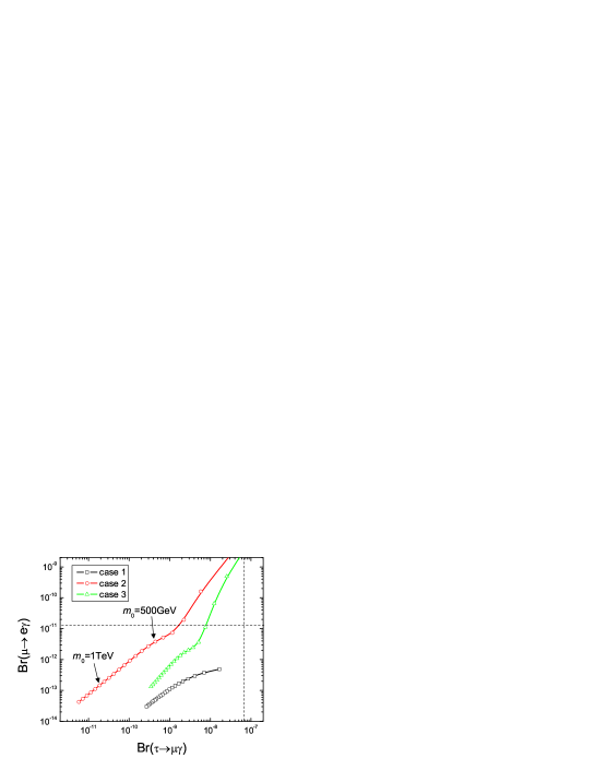
Figure 3: The branching ratios of the LFV decays are plotted. In the plot, slepton mass at cutoff scale is varied with 50 GeV steps. The detailed parameters we used are given in the text. Dashed lines are drawn for the current experimental bounds at 90%CL. The lines are plotted for the following cases: (Case 1) $Y_{\nu_{\tau}}=Y_{t}$ and $c=0$, (Case 2) $Y_{\nu_{\tau}}=0.1\,Y_{t}$ and $c=0.1$, (Case 3) $Y_{\nu_{\tau}}=Y_{t}$ and $c=0.1$. $c$ is the coefficient given in the Eq.(19).

We plot the branching ratios of $\tau\rightarrow\mu\gamma$ and $\mu\rightarrow e\gamma$ in Fig. 3. For the SUSY breaking parameters, we assume that $m_{\tilde{\ell}}^{2}{}_{ij}=m_{\tilde{e}}^{2}{}_{ij}=m_{0}^{2}\,{\bf 1}$ and $A_{e}=A_{0}Y_{e}+A_{e}^{U}$ at the cutoff scale $M_{*}$ as we have mentioned. In the intersecting D-brane models, the SUSY breaking scalar mass is not necessarily universal for different representation, though the flavor degeneracy is achieved. We assume that the left and right scalar masses to be same just for simplicity. The cutoff scale is related to the string scale and the volume of the extra dimensions. We choose that $M_{*}=10^{17}$ GeV in the calculation. We take gaugino mass $M_{1/2}=500$ GeV at $M_{*}$, $A_{0}=500$ GeV and Higgsino mass $\mu=500$ GeV (we choose the signature of $\mu$ to make the SUSY contribution of anomalous magnetic moment of muon [27] to be positive). The value of $\tan\beta$ which is the ratio of the vacuum expectation values for Higgs fields is taken to be $\tan\beta=50$. The amplitudes for the LFV decays are naively proportional to $\tan\beta$, thus the branching ratios are $\propto\tan^{2}\beta$. In the Fig.3, we vary $m_{0}$ in 50 GeV steps and the maximal value is $m_{0}=1250$ GeV (which corresponds to the lightest stau of about 1 TeV). In order to show the results clearly, we assume that the LFV sources are only the Dirac neutrino Yukawa coupling and the $U$-moduli contribution in $A_{e}$. We neglect the sources arising in the Majorana couplings (Eq.(14)) by assuming them to be small. In the plot, Dirac neutrino coupling is the only source in the case 1. We take the largest right-handed Majorana mass to be $10^{15}$ GeV. In the case 2, the $U$-moduli contribution is the dominant source of LFV. The case 3 has both sources. It is easy to see that the neutrino Dirac couplings makes the branching ratio Br($\tau\rightarrow\mu\gamma$) large. This is because that these couplings generate the off-diagonal (2,3) element of the left-handed slepton mass matrix and contributes to the chargino diagram of $\tau\rightarrow\mu\gamma$. The flavor violation source arising from the neutrino Dirac couplings can contribute to the $\mu\rightarrow e\gamma$ decay since the (1,3) element is also generated, but this element is smaller than the (2,3) element. If we switch on the $U$-moduli contribution, the (1,3) element can be comparable to the (2,3) element and thus, the $U$-moduli contribution increases the $\mu\rightarrow e\gamma$ decay rate more than the $\tau\rightarrow\mu\gamma$ decay rate. The reason for the behavior of the lines being different (in the Fig.3) when $m_{0}$ is smaller than 400 GeV is that the Bino-Bino diagram dominates rather than the chargino diagram due to the large left-right mixings of the slepton. The qualitative behaviors of the cases 1 and 2 are not very different even if we change the numerical parameters, but the case 3 depends much on the initial condition such as $A_{0}$ and $\mu$ since there can be a slight cancellation among the diagrams. The right- and left-handed lepton decays do not have interference, and a huge cancellations among the diagram for the branching ratios happen hardly.

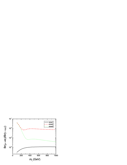
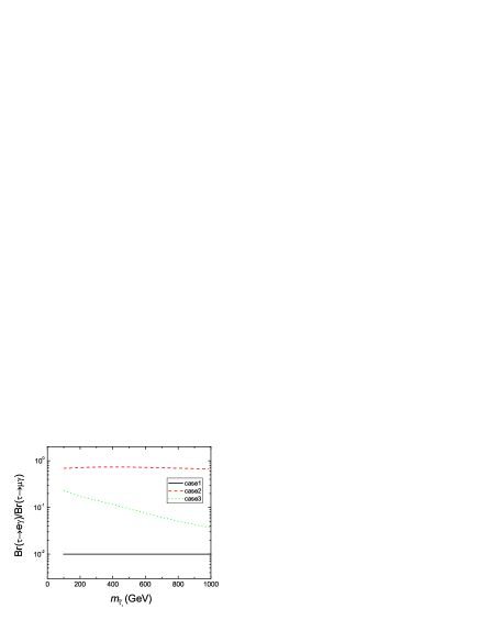
Figure 4: Plots for the ratio of branching ratios. The lines are plotted for the following cases: (Case 1) $Y_{\nu_{\tau}}=Y_{t}$ and $c=0$, (Case 2) $Y_{\nu_{\tau}}=0.1\,Y_{t}$ and $c=0.1$, (Case 3) $Y_{\nu_{\tau}}=Y_{t}$ and $c=0.1$.

The branching ratio for each decay mode depends on the initial conditions. However, as shown in the Fig.4, the ratio of the branching ratios can be a good prediction for different LFV sources. In the figure, we use the same initial conditions as before. The ratio of the branching ratio is almost determined by the mixing angles in $V_{L}^{e\nu}$ for the case 1 and the ratio of the (1,3) and the (2,3) elements in the $A_{e}^{U}$ for the case 2. Therefore, if all the branching ratios for $\tau\rightarrow\mu\gamma$, $\tau\rightarrow e\gamma$ and $\mu\rightarrow e\gamma$ are measured, we can obtain important information to identify the LFV source. In fact, the following relations are satisfied approximately: Br($\mu\rightarrow e\gamma$)/Br($\tau\rightarrow\mu\gamma)\sim(\theta_{13}^{e})^{2}$/Br($\tau\rightarrow\mu\bar{\nu}_{\mu}\nu_{\tau})$ for the case 1, $\sim(A_{e}{}_{13}/A_{e}{}_{33})^{2}$/Br($\tau\rightarrow\mu\bar{\nu}_{\mu}\nu_{\tau}$) for the case 2 and Br($\tau\rightarrow e\gamma$)/Br($\tau\rightarrow\mu\gamma)\sim(\theta_{13}^{e}/\theta_{23}^{e})^{2}$ for the case 1, $\sim(A_{e}{}_{13}/A_{e}{}_{23})^{2}$ for case 2. In the case 3, the LFV sources are mixed, we do not have such simple expressions. These ratios of the branching ratios do not depend much on the initial conditions such as $m_{0}$, $A_{0}$, $M_{1/2}$, $\mu$ and $\tan\beta$ if the chargino diagram provides the dominant contribution. When the sleptons are light and the left-right mixing becomes large, the Bino diagram can contribute to $\mu\rightarrow e\gamma$ and bends the lines for the ratio Br($\mu\rightarrow e\gamma$)/Br($\tau\rightarrow\mu\gamma$) in the Fig.4 for smaller $m_{0}$.

The large Majorana couplings $f$ can contribute to the LFV decays due to its off-diagonal terms. If the type II seesaw dominates the neutrino masses, the ratios of the branching ratios are almost determined by the neutrino mixings when the Majorana couplings are the dominant sources of the LFV decays. In this case, the ratio Br$(\mu\rightarrow e\gamma)$/Br$(\tau\rightarrow\mu\gamma$) is about $U_{e3}^{2}$/Br($\tau\rightarrow\mu\bar{\nu}_{\mu}\nu_{\tau}$) while the ratio Br$(\tau\rightarrow e\gamma)$/Br$(\tau\rightarrow\mu\gamma)$ is about $(U_{e3}/U_{\mu 3})^{2}\simeq(\theta_{12}^{e})^{2}$. The first value is similar to the pure $U$-moduli case (case 2) and the second value is similar to the Dirac neutrino case (case 1). Thus the observation of the ratios can sort out the LFV sources.

Usually, the 13 mixing is smaller than the 23 mixing in $V_{L}^{e\nu}$ or $U_{L}^{e}$, even if we use a different setup, and thus the $\tau\rightarrow e\gamma$ decay rate is expected to be smaller than the $\tau\rightarrow\mu\gamma$ decay rate. However, if the $U$-moduli contribution dominates, those two decay rates can be comparable since the (1,3) and the (2,3) elements in $A_{e}^{U}$ are comparable. So measuring the ratio Br$(\tau\rightarrow e\gamma)$/Br$(\tau\rightarrow\mu\gamma)$ is very important to see the presence of the $U$-moduli contribution.

5.2 EDM

The other important observables to select the sources of LFV are the EDMs of the electron and the muon. If the trilinear scalar coupling $A_{0}$ and the Higgsino mass $\mu$ are complex parameters, the EDMs can be large even if we do not have any source of LFV violation. However, if those are complex in general, the EDM of the electron can be too large compared to the experimental bounds when the slepton masses are less than around 1 TeV [28]. Thus a cancellation is needed in that case to satisfy the bound [29]. It is unnatural to have cancellations for both the electron and the muon and thus the muon EDM will be large enough to be detected in the future experiments [30]. It is often assumed that the $A_{0}$ and $\mu$ are real to satisfy the experimental bound naturally. In this case, the amount of EDMs are related to the source of LFV.

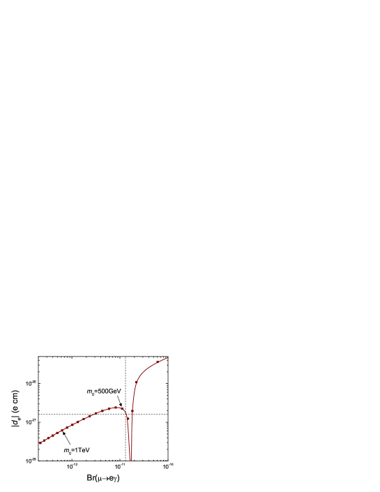
Figure 5: Plots for electron EDM and branching ratio of $\mu\rightarrow e\gamma$. In the plot, the slepton mass at the cutoff scale is varied with 50 GeV steps. Dashed lines are drawn for the current experimental bounds at 90%CL.

Let us suppose that $A_{0}$ and $\mu$ are real and all the CP phases are in the Yukawa couplings. The EDMs are imaginary part of the amplitude of the loop diagram. Since in the diagram, where the chirality flipping vertex does not include CP phase in generation mixings, the Bino-Bino diagram dominates the EDM calculation. The imaginary parts of $(A_{e})_{11}$ and $(A_{e})_{12}m_{\tilde{e}}^{2}{}_{21}$ etc in the basis where the charged-lepton matrix is real and diagonal can be also important. However, if the $A$-term is proportional to the Yukawa coupling, such imaginary parts are small. The electron EDM can be proportional to $\mu\tan\beta\,m_{\tau}$ when the (1,3) mixings for both left- and right-handed slepton mass matrices are generated. If the neutrino Dirac Yukawa coupling is the only source of LFV, the off-diagonal elements of right-handed slepton mass matrix are very small and consequently, the EDM of the electron is small, $d_{e}\sim 10^{-33}\,e\,$cm. Even in the type I seesaw with generic right-handed Majorana mass matrix, the electron EDM is at most $d_{e}\sim 10^{-29}\,e\,$cm [31]. If the $U$-moduli is a source of LFV processes, the off-diagonal elements for both left- and right-handed slepton mass matrices can be generated and thus the electron EDM can be enhanced to reach the current experimental bound $|d_{e}|<1.6\times 10^{-27}\,e\,$cm [24]. Hence, the electron EDM is an important observable to see whether the LFV arises from only the neutrino Dirac Yukawa coupling or not.

In the intersecting D-brane models, if we assume that the $F$-term of moduli does not have any phase then $A_{0}$ does not get any phase. The phase of the Higgsino mass depends on the model, but it may be related to the SUSY breaking parameters and thus can be real in such an assumption. On the other hand, the Yukawa couplings can be complex if we include the Wilson line phases in the theta function [9]. Then the $U$-moduli contribution of the $A$ term can be generically complex while $A_{0}$ is real.

We plot the electron EDM and the branching ratio of $\mu\rightarrow e\gamma$ in the Fig.5 in the case where the $U$-moduli contribution is large enough using the same input for the SUSY breaking parameters as before. In this case, the values different from what has be shown for the neutrino Dirac Yukawa couplings do not change the plot very much since the chargino diagram does not contribute to the EDM. In general each component of $A_{e}^{U}$ can be complex independently. In the plot, we take the overall factor for the $U$ moduli contribution $c$ to be pure imaginary for simplicity. The EDM can easily saturate the current experimental bound. For larger $m_{0}$, the $A_{e}v_{d}$ contribution is larger compared to the $\mu\tan\beta\,m_{\tau}$ part in the left-right slepton mixing while for smaller $m_{0}$ ($<400$ GeV), the $\mu\tan\beta\,m_{\tau}$ contribution becomes larger than the $A_{e}v_{d}$ part. This is because $\mu\tan\beta\,m_{\tau}$ contribution needs triple mass insertion in the Bino diagram and thus the amplitude is suppressed by larger power of $m_{0}$ than the $A_{e}v_{d}$ contribution which can be produced by a single mass insertion.

The presence of large complex Majorana couplings can also saturate the EDM bound when $\mu\tan\beta\,m_{\tau}$ contribution is large for light sleptons. The $A_{e}v_{d}$ part is small when $U$-moduli contribution is absent. When sleptons are heavy (depending on $\mu\tan\beta$), the $\mu\tan\beta\,m_{\tau}$ contribution is suppressed due to the triple mass insertion and thus the EDM becomes smaller for a fixed Br$(\mu\rightarrow e\gamma)$, comparing to the case when the $U$-moduli contribution is dominant.

The muon EDM is $d_{\mu}\sim 10^{-26}-10^{-24}\,e\,$cm as long as the bound for $d_{e}$ is satisfied and there is no huge cancellation in $d_{e}$. The ratio of the EDMs does not depend on the ratio of the corresponding charged lepton masses, $d_{\mu}/d_{e}\neq m_{\mu}/m_{e}$.

6 Conclusions

We have discussed the flavor sector in the intersecting D-brane models. In the D-brane models, the low energy effective action for the zero modes such as particles in MSSM can be calculated using the geometrical parameters. The neutrino mixing is elegantly realized in the context of the almost rank 1 Yukawa matrix. The flavor degeneracy of SUSY breaking scalar masses are realized when the generation is simply replicated at the intersection of the D-branes. The non-proportional part of the scalar trilinear coupling is obtained when the $F$-term of the $U$-moduli is not zero.

Emphasizing the flavor degeneracy of SUSY breaking scalar masses in these models, we study the lepton flavor violating processes. The $U$-moduli contribution of the scalar trilinear coupling can be the source of lepton flavor violation as well as the neutrino Dirac and Majorana Yukawa couplings which are included in the MSSM plus right-handed neutrino.

We calculate the branching ratios of the LFV decays and the EDM of the electron $d_{e}$. The observations of the $d_{e}$ and the ratio of the branching ratios for $\mu\rightarrow e\gamma$, $\tau\rightarrow\mu\gamma$ and $\tau\rightarrow e\gamma$ are important to sort out the sources of LFV as shown in the Fig.4.

The bound for the EDM of the electron can be improved to $d_{e}\sim 10^{-32}\,e\,$cm in the planned experiments [32]. Under the assumption that the SUSY breaking parameters and the Higgsino mass are real, it is possible to see whether we have any source of LFV in addition to the Dirac neutrino Yukawa couplings in mSUGRA. The $U$-moduli contribution in our scheme can saturate the current experimental bounds for $d_{e}<1.6\times 10^{-27}\,e\,$cm as well as the Br($\mu\rightarrow e\gamma$). The current bound for the branching ratio is Br($\mu\rightarrow e\gamma)<1.2\times 10^{-11}$ and it can go down to $\sim 5\times 10^{-14}$ in the near future [33].

The $U$-moduli contribution in the trilinear scalar coupling can make Br($\tau\rightarrow e\gamma$)/Br($\tau\rightarrow\mu\gamma$) to be order 1. In the models where the Dirac neutrino or the Majorana couplings are the primary sources of LFV, this ratio is much smaller than 1. In order to completely sort out the LFV sources from the ratio of the branching ratios, the $\tau$ LFV decays with branching ratio $10^{-9}-10^{-10}$ need to be at least measured. At present, the upper bound on the branching ratio of $\tau\rightarrow\mu\gamma$ is $6.8\times 10^{-8}$ [15] and this bound can be improved to $10^{-10}$ at the ILC-Super B [34].

References

- [1] F. Gabbiani and A. Masiero, Nucl. Phys. B 322, 235 (1989); J. S. Hagelin, S. Kelley and T. Tanaka, Nucl. Phys. B 415, 293 (1994); F. Gabbiani, E. Gabrielli, A. Masiero and L. Silvestrini, Nucl. Phys. B 477, 321 (1996) [hep-ph/9604387].
- [2] A. H. Chamseddine, R. Arnowitt and P. Nath, Phys. Rev. Lett. 49, 970 (1982); R. Barbieri, S. Ferrara and C. A. Savoy, Phys. Lett. B 119, 343 (1982); L. J. Hall, J. D. Lykken and S. Weinberg, Phys. Rev. D 27, 2359 (1983); E. Cremmer, P. Fayet and L. Girardello, Phys. Lett. B 122, 41 (1983); N. Ohta, Prog. Theor. Phys. 70, 542 (1983).
- [3] M. Berkooz, M. R. Douglas and R. G. Leigh, Nucl. Phys. B 480, 265 (1996) [hep-th/9606139]. H. Arfaei and M. M. Sheikh Jabbari, Phys. Lett. B 394, 288 (1997) [hep-th/9608167].
- [4] R. Blumenhagen, L. Goerlich, B. Kors and D. Lust, JHEP 0010, 006 (2000) [hep-th/0007024]; R. Blumenhagen, B. Kors and D. Lust, JHEP 0102, 030 (2001) [hep-th/0012156]; G. Aldazabal, S. Franco, L. E. Ibanez, R. Rabadan and A. M. Uranga, JHEP 0102, 047 (2001) [hep-ph/0011132].
- [5] For a reivew, R. Blumenhagen, M. Cvetic, P. Langacker and G. Shiu, hep-th/0502005.
- [6] R. Blumenhagen, B. Kors, D. Lust and T. Ott, Nucl. Phys. B 616, 3 (2001) [hep-th/0107138]; M. Cvetic, G. Shiu and A. M. Uranga, Phys. Rev. Lett. 87, 201801 (2001) [hep-th/0107143]; Nucl. Phys. B 615, 3 (2001) [hep-th/0107166]; D. Cremades, L. E. Ibanez and F. Marchesano, JHEP 0207, 022 (2002) [hep-th/0203160]; M. Cvetic, P. Langacker and G. Shiu, Nucl. Phys. B 642, 139 (2002) [hep-th/0206115]; G. Honecker and T. Ott, Phys. Rev. D 70, 126010 (2004) [hep-th/0404055]; C. Kokorelis, hep-th/0406258; hep-th/0410134; Nucl. Phys. B 732, 341 (2006) [hep-th/0412035]; C. M. Chen, T. Li and D. V. Nanopoulos, Nucl. Phys. B 732, 224 (2006) [hep-th/0509059]; G. K. Leontaris and J. Rizos, Phys. Lett. B 632, 710 (2006) [hep-ph/0510230].
- [7] C. Kokorelis, JHEP 0208, 018 (2002) [hep-th/0203187]; J. R. Ellis, P. Kanti and D. V. Nanopoulos, Nucl. Phys. B 647, 235 (2002) [hep-th/0206087]; M. Axenides, E. Floratos and C. Kokorelis, JHEP 0310, 006 (2003) [hep-th/0307255]; C. M. Chen, G. V. Kraniotis, V. E. Mayes, D. V. Nanopoulos and J. W. Walker, Phys. Lett. B 611, 156 (2005) [hep-th/0501182]; Phys. Lett. B 625, 96 (2005) [hep-th/0507232]; C. M. Chen, V. E. Mayes and D. V. Nanopoulos, Phys. Lett. B 633, 618 (2006) [hep-th/0511135].
- [8] M. Cvetic, T. Li and T. Liu, Nucl. Phys. B 698, 163 (2004) [hep-th/0403061]; F. Marchesano and G. Shiu, Phys. Rev. D 71, 011701 (2005) [hep-th/0408059]; JHEP 0411, 041 (2004) [hep-th/0409132]; M. Cvetic and T. Liu, Phys. Lett. B 610, 122 (2005) [hep-th/0409032]; M. Cvetic, T. Li and T. Liu, Phys. Rev. D 71, 106008 (2005) [hep-th/0501041]; C. M. Chen, T. Li and D. V. Nanopoulos, Nucl. Phys. B 740, 79 (2006) [hep-th/0601064].
- [9] D. Cremades, L. E. Ibanez and F. Marchesano, JHEP 0307, 038 (2003) [hep-th/0302105]; JHEP 0405, 079 (2004) [hep-th/0404229].
- [10] M. Cvetic and I. Papadimitriou, Phys. Rev. D 68, 046001 (2003) [hep-th/0303083]; S. A. Abel and A. W. Owen, Nucl. Phys. B 663, 197 (2003) [hep-th/0303124]; Nucl. Phys. B 682, 183 (2004) [hep-th/0310257]; D. Lust, P. Mayr, R. Richter and S. Stieberger, Nucl. Phys. B 696, 205 (2004) [hep-th/0404134]; S. A. Abel and B. W. Schofield, JHEP 0506, 072 (2005) [hep-th/0412206]; T. Higaki, N. Kitazawa, T. Kobayashi and K. j. Takahashi, Phys. Rev. D 72, 086003 (2005) [hep-th/0504019]; M. Bertolini, M. Billo, A. Lerda, J. F. Morales and R. Russo, hep-th/0512067.
- [11] B. Kors and P. Nath, Nucl. Phys. B 681, 77 (2004) [hep-th/0309167].
- [12] P. G. Camara, L. E. Ibanez and A. M. Uranga, Nucl. Phys. B 689, 195 (2004) [hep-th/0311241]; D. Lust, S. Reffert and S. Stieberger, Nucl. Phys. B 706, 3 (2005) [hep-th/0406092]; Nucl. Phys. B 727, 264 (2005) [hep-th/0410074]; L. E. Ibanez, Phys. Rev. D 71, 055005 (2005) [hep-ph/0408064]; A. Font and L. E. Ibanez, JHEP 0503, 040 (2005) [hep-th/0412150].
- [13] N. Chamoun, S. Khalil and E. Lashin, Phys. Rev. D 69, 095011 (2004) [hep-ph/0309169]; S. A. Abel, O. Lebedev and J. Santiago, Nucl. Phys. B 696, 141 (2004) [hep-ph/0312157]; N. Kitazawa, Nucl. Phys. B 699, 124 (2004) [hep-th/0401096]; N. Kitazawa, T. Kobayashi, N. Maru and N. Okada, Eur. Phys. J. C 40, 579 (2005) [hep-th/0406115]; T. Noguchi, hep-ph/0410302.
- [14] B. Dutta and Y. Mimura, Phys. Lett. B 633, 761 (2006) [hep-ph/0512171].
- [15] M. L. Brooks et al. [MEGA Collaboration], Phys. Rev. Lett. 83, 1521 (1999) [hep-ex/9905013]; K. Abe et al. [Belle Collaboration], Phys. Rev. Lett. 92, 171802 (2004) [hep-ex/0310029]; B. Aubert et al. [BABAR Collaboration], Phys. Rev. Lett. 95, 041802 (2005) [hep-ex/0502032]; Phys. Rev. Lett. 96, 041801 (2006) [hep-ex/0508012].
- [16] F. Borzumati and A. Masiero, Phys. Rev. Lett. 57, 961 (1986); J. Hisano, T. Moroi, K. Tobe, M. Yamaguchi and T. Yanagida, Phys. Lett. B 357, 579 (1995) [hep-ph/9501407].
- [17] J. C. Pati and A. Salam, Phys. Rev. D 10, 275 (1974).
- [18] M. Cvetic, P. Langacker, T. j. Li and T. Liu, Nucl. Phys. B 709, 241 (2005) [hep-th/0407178].
- [19] M. Cvetic, P. Langacker and J. Wang, Phys. Rev. D 68, 046002 (2003) [hep-th/0303208].
- [20] A. Brignole, L. E. Ibanez and C. Munoz, hep-ph/9707209.
- [21] C. Giunti and M. Tanimoto, Phys. Rev. D 66, 053013 (2002) [hep-ph/0207096]; P. H. Frampton, S. T. Petcov and W. Rodejohann, Nucl. Phys. B 687, 31 (2004) [hep-ph/0401206]; Z. z. Xing, Phys. Lett. B 618, 141 (2005) [hep-ph/0503200]. A. Datta, L. Everett and P. Ramond, Phys. Lett. B 620, 42 (2005) [hep-ph/0503222]; J. Harada, hep-ph/0512294.
- [22] P. Minkowski, Phys. Lett. B 67, 421 (1977); T. Yanagida, in proc. of KEK workshop, eds. O. Sawada and S. Sugamoto (Tsukuba, 1979); M. Gell-Mann, P. Ramond and R. Slansky, in Supergravity, eds. P. van Nieuwenhuizen and D. Z. Freedman (North-Holland, Amsterdam, 1979); R. N. Mohapatra and G. Senjanović, Phys. Rev. Lett. 44, 912 (1980).
- [23] J. Schechter and J. W. F. Valle, Phys. Rev. D 22, 2227 (1980); R. N. Mohapatra and G. Senjanovic, Phys. Rev. D 23, 165 (1981); G. Lazarides, Q. Shafi and C. Wetterich, Nucl. Phys. B 181, 287 (1981).
- [24] B. C. Regan, E. D. Commins, C. J. Schmidt and D. DeMille, Phys. Rev. Lett. 88, 071805 (2002).
- [25] L. J. Hall, V. A. Kostelecky and S. Raby, Nucl. Phys. B 267, 415 (1986); R. Barbieri and L. J. Hall, Phys. Lett. B 338, 212 (1994) [hep-ph/9408406]; R. Barbieri, L. J. Hall and A. Strumia, Nucl. Phys. B 445, 219 (1995) [hep-ph/9501334]; J. Hisano, T. Moroi, K. Tobe and M. Yamaguchi, Phys. Lett. B 391, 341 (1997) [hep-ph/9605296]; J. Hisano and D. Nomura, Phys. Rev. D 59, 116005 (1999) [hep-ph/9810479].
- [26] K. S. Babu, B. Dutta and R. N. Mohapatra, Phys. Lett. B 458, 93 (1999) [hep-ph/9904366]; N. G. Deshpande, B. Dutta and E. Keith, Phys. Rev. D 54, 730 (1996) [hep-ph/9512398].
- [27] H. N. Brown et al. [Muon g-2 Collaboration], Phys. Rev. Lett. 86, 2227 (2001) [hep-ex/0102017].
- [28] E. Franco and M. L. Mangano, Phys. Lett. B 135, 445 (1984); P. Nath, Phys. Rev. Lett. 66, 2565 (1991); Y. Kizukuri and N. Oshimo, Phys. Rev. D 46, 3025 (1992).
- [29] T. Ibrahim and P. Nath, Phys. Rev. D 58, 111301 (1998) [hep-ph/9807501]; M. Brhlik, G. J. Good and G. L. Kane, Phys. Rev. D 59, 115004 (1999) [hep-ph/9810457]; E. Accomando, R. Arnowitt and B. Dutta, Phys. Rev. D 61, 115003 (2000) [hep-ph/9907446].
- [30] Y. K. Semertzidis et al., hep-ph/0012087.
- [31] J. R. Ellis, J. Hisano, M. Raidal and Y. Shimizu, Phys. Rev. D 66, 115013 (2002) [hep-ph/0206110].
- [32] S. K. Lamoreaux, nucl-ex/0109014.
- [33] M. Grassi [MEG Collaboration], Nucl. Phys. Proc. Suppl. 149, 369 (2005).
- [34] Talk by M. Giorgi at the 2nd Workshop on Super B-Factory, 16-18 March 2006, Frascati, Italy [http://www.lnf.infn.it/conference/superb06/talks/Giorgi.ppt]; The SuperKEKB can improve the branching ratio to several [http://belle.kek.jp/superb/].