Quark masses and mixings in $E_{6}\times S_{3}$ : a montecarlo approach

Abstract

Recently in Ref. Caravaglios:2005gf has been proposed a GUT model for fermion masses and mixings with spontaneously broken S₃ discrete flavor symmetry, where S₃ is the permutation group of three objects. The S₃ breaking pattern in the quark sector is not studied and need further investigation. Since in such a model the number of free parameters is greater than the number of experimental observables, an analytical fit of all the parameters is impossible. To go forward with the model building and to deal with this problem we have used a statistical analysis. We have found that S₃ is totally broken and the up-type quarks matrix is approximatively diagonal while down-type quarks matrix is not symmetric and it is parametrized by three couplings, $g^{d},~{}g_{L}^{d}$ and $g_{3}^{d}$. It has been found that $g_{L}^{d}$ is slightly smaller than $g^{d}=1$ and it is of order one, while $g_{3}^{d}\sim\lambda^{3}$ where $\lambda$ is the Cabibbo angle. An analytical study of the dependence of $V_{cb}$ and $V_{ub}$ from the couplings $g_{L}^{d}$ and $g_{3}^{d}$ is also presented.

I Introduction

In third quantization Caravaglios:2002ws we can explain the origin of the fermion families and the origin of the permutation symmetry between them. Third quantization is an extension of the quantum field theory where the fields are treated as well as particles in second quantization. Discrete flavor symmetries, like the group of permutation of three objects $S_{3}$, are very interesting since they can naturally explain neutrino mixing angles and mass hierarchies, for instance see Ref. Harrison:2002er . Some recent reviews in the study of hierarchical structure of fermion masses in the Standard Model and its extensions are reported in Ref Fritzsch:1999ee . Indications toward grand unification gauge theory (GUT), is the phenomenological tendency to unify of the gauge couplings, and the theoretical implicit possibility to explain charge quantization and anomaly cancellation. In Ref. Caravaglios:2005gf it has been proposed a model based on $E_{6}\times S_{3}$ in order to arrange quark, lepton and neutrino masses and mixings. Minimal GUT models give strong relations between quarks and leptons Yukawa matrices. For example in minimal SO(10) models up quarks Yukawa matrix is equal to the Dirac neutrino Yukawa matrix. However quarks and neutrinos mass and mixing hierarchies are very different. In fact, neutrino oscillation data show a maximal atmospheric angle, large solar angle and $\theta_{13}$ close to zero, see Ref. Fogli:2005cq . In contrast the greatest angle in the quark sector, namely the Cabibbo one, is smaller than the corresponding leptonic mixing angle, see Ref. Charles:2004jd . Phenomenological quark/lepton difference seems in contrast with GUT features. Even though in $E_{6}$ models it is possible to make a distinction between charged fermions and neutrinos as showed in Ref. Caravaglios:2005gf . Authors evidenced this possibility by means of the two standard model singlets contained in $E_{6}$. In such a model quarks Yukawas only emerge after $S_{3}$ symmetry is broken by not renormalizable dimension five operators, while renormalizable operators only contribute to Dirac neutrino Yukawas. However the study of $S_{3}$ breaking pattern in the quark sector has not been accomplished in Ref. Caravaglios:2005gf and it will be performed in this paper.

We will show that in our model up and down-type quark mass matrices are parametrized both by five complex couplings and three real parameters. Since the number of free parameters in the quark sector of the model is larger than the number of experimental data, a direct fit is impossible. One possibility to deal with this problem, is comparing the theoretical expectations with the experimental data by means of a montecarlo method (see Ref. Caravaglios:2002br ) that assigns a probability weight to points in the parameter space of the model according to a goodness of fit criterion. In this way we find the statistically preferred textures of the mass matrices for up and down-type quarks. In particular we select a large number of points in the parameters space initially uniformed distributed. After applying the experimental constrains, not all the selected points agree with data. To apply the experimental constrains it is been used the $\chi^{2}$ function defined as below

$$\chi^{2}(O^{{\rm t}h})=\sum_{i}\left(\frac{O^{{\rm t}h}_{i}-O^{{\rm e}xp}_{i}}{\sigma^{{{\rm e}xp}}_{i}}\right)^{2}$$ (1)

where $O^{{\rm e}xp}_{i}$ and $\sigma^{{\rm e}xp}_{i}$ are respectively the experimental data and their standard deviations while $O^{{\rm t}h}_{i}$ are the corresponding values predicted by the model. The points in the configuration space are statistically taken with a probability proportional to exp$(-\chi^{2}/2)$. After experimental constrains are applied we get a not uniform distribution in the parameters space. Regions very high populated will be interpreted statistically more probable than regions with low density population. This method selects models statistically preferred by data giving the magnitude of the fitting parameters.

The paper is organized as follows: in section II we give the up and down quark mass matrices textures derived by $E_{6}\times S_{3}$ model, in section III we introduce the numerical method used and we report the results, in section IV we give the conclusions.

II S₃ symmetry and the quark mass matrices

The discrete group of permutation of three objects, called $S_{3}$, contains six elements and it has four irreducible representations, namely a doublet 2, one symmetric singlet 1 and one antisymmetric singlet ${\bf 1^{\prime}}$, see for instance Ref. s3e . The product of two doublets is

$${\bf 2\times 2=2+1+1^{\prime}}.$$ (2)

In particular, if $(\chi^{a}_{1},\chi^{a}_{2})$ and $(\chi^{b}_{1},\chi^{b}_{2})$ are two $S_{3}$ doublets, their product is

$$\chi_{D} = \frac{1}{\sqrt{2}}(\chi^{a}_{2}~{}\chi^{b}_{1}+\chi^{a}_{1}~{}\chi^{b}_{2}~{},~{}\chi^{a}_{1}~{}\chi^{b}_{1}-\chi^{a}_{2}~{}\chi^{b}_{2})$$

$$\chi_{S} = \frac{1}{\sqrt{2}}(\chi^{a}_{1}~{}\chi^{b}_{1}+\chi^{a}_{2}~{}\chi^{b}_{2})$$

$$\chi_{A} = \frac{1}{\sqrt{2}}(\chi^{a}_{2}~{}\chi^{b}_{1}-\chi^{a}_{1}~{}\chi^{b}_{2})$$

where $\chi_{D}$ is the doublet of eq.(2) while $\chi_{S}$ and $\chi_{A}$ are respectively the symmetric and the antisymmetric singlets.

Let be $\psi_{1},~{}\psi_{2}$ and $\psi_{3}$ three fields belonging to a triplet reducible representation 3 of $S_{3}$. Then the triplet reducible representation decompisition is 3=2+1:

$$\psi_{S} = \frac{1}{\sqrt{3}}(\psi_{1}+\psi_{2}+\psi_{3})$$

$$\psi_{D} = \left(\frac{1}{\sqrt{2}}(-\psi_{2}+\psi_{3})~{},~{}\frac{1}{\sqrt{6}}(-2~{}\psi_{1}+\psi_{2}+\psi_{3})\right)$$ (3)

where $\psi_{S}$ is a symmetric singlet of $S_{3}$ and $\psi_{D}$ is a doublet of $S_{3}$.

In $E_{6}\times S_{3}$ model of Ref. Caravaglios:2005gf the quarks Yukawa matrices come from dimension five operators below

$$L_{Yuk}=\sum_{i\neq j\neq k}\left(g_{ijk}^{u}~{}H_{u}\bar{Q}_{Li}u_{Rj}\phi_{k}^{u}+g_{ijk}^{d}~{}H_{d}\bar{Q}_{Li}d_{Rj}\phi_{k}^{d}\right)+{\rm h.c.}$$ (4)

where $i,j,k=1,2,3$, the scalar fields $\phi^{u,d}_{i}$ are Standard Model singlets, $H_{u}$ and $H_{d}$ are electroweak doublets, $Q_{Li}$ are the left-handed fermion electroweak doublets while $u_{Ri}$ and $d_{Ri}$ are right-handed fermion electroweak singlets and $g_{ijk}^{u,d}$ are $S_{3}$ tensors. We assign the left-handed fermions, the right-handed fermions and the scalar $\phi^{u,d}_{i}$ to triplet reducible representations of $S_{3}$, namely

$$Q_{L}=(u_{i},d_{i})_{L}~{}\sim~{}{\bf 3}~{},~{}~{}u_{R~{}i}~{}\sim~{}{\bf 3}~{},~{}~{}d_{R~{}i}~{}\sim~{}{\bf 3},~{}\phi_{i}^{u,d}~{}\sim~{}{\bf 3}.$$

The Higgs electroweak doublets are $S_{3}$ symmetric singlets, $H_{u,d}\sim{\bf 1}$. With this assignment both the operators in eq. (4) transform with respect to the permutation group as follows

$${\bf 3_{a}\times 3_{b}\times 3_{c}\times 1}={\bf(2_{a}+1_{a})\times(2_{b}+1_{b})\times(2_{c}+1_{c})\times 1}=$$ (5)

$$={\bf(2_{a}\times 2_{b}\times 2_{c}~{}+~{}2_{a}\times 2_{b}\times 1_{c}+2_{a}\times 1_{b}\times 2_{c}}++{\bf 1_{a}\times 2_{b}\times 2_{c}+1_{a}\times 1_{b}\times 1_{c})\times 1}.$$

First four terms of five in eq.(5) contain the symmetric and the antisymmetric singlets, see eq. (2). Only symmetric singlets give $S_{3}$ invariant interactions because we have chosen the Higgs fields in symmetric singlet representation and 1$\times$1${}^{\prime}=$ 1^′. Consequently Yukawa interactions in eq. (4) give only five terms $S_{3}$ invariant both in up and down quark sectors.

The lagrangian is, see also Ref. s3c ,

$$L_{yuk} = (c_{1}^{d}~{}\overline{Q}_{D}d_{D}\phi_{D}+c_{2}^{d}~{}\overline{Q}_{D}d_{S}\phi_{D}+c_{3}^{d}~{}\overline{Q}_{S}d_{D}\phi_{D}+c_{4}^{d}~{}\overline{Q}_{D}d_{D}\phi_{S}+c_{5}^{d}~{}\overline{Q}_{S}d_{S}\phi_{S})~{}H^{d}$$ (6)

$$+ (c_{1}^{u}~{}\overline{Q}_{D}u_{D}\phi_{D}+c_{2}^{u}~{}\overline{Q}_{D}u_{S}\phi_{D}+c_{3}^{u}~{}\overline{Q}_{S}u_{D}\phi_{D}+c_{4}^{u}~{}\overline{Q}_{D}u_{D}\phi_{S}+c_{5}^{u}~{}\overline{Q}_{S}u_{S}\phi_{S})~{}H^{u}$$

$$+$$ h.c.

where $Q_{D},~{}d_{D},~{}u_{D},~{}\phi_{D},~{}Q_{S},~{}d_{S},~{}\phi_{S}$ and $u_{S}$ follow from relations in eq.(3) and $c_{i}^{u,d}$ are arbitrary complex constants. With the following redefinition of the complex constants

$$\begin{array}[]{ccc}c_{1}&=&\sqrt{\frac{2}{3}}~{}(g-g_{2}-g_{L}-g_{R}+g_{3})\\ c_{2}&=&\sqrt{\frac{2}{3}}~{}(g-g_{2}+2~{}g_{L}-g_{R}-g_{3})\\ c_{3}&=&\sqrt{\frac{2}{3}}~{}(g-g_{2}-g_{L}+2~{}g_{R}-g_{3})\\ c_{4}&=&\sqrt{\frac{2}{3}}~{}(g+2~{}g_{2}-g_{L}-g_{R}-g_{3})\\ c_{5}&=&\frac{1}{\sqrt{3}}~{}g+2(g_{2}+g_{L}+g_{R}+g_{3})\\ \end{array}$$ (7)

and using relations in eq. (3), from eq. (6) we get the following down quarks lagrangian

$$\sum_{i\neq j\neq k}\left(g\bar{d}_{L}^{i}d_{R}^{i}H\phi_{i}+g_{2}\bar{d}_{L}^{i}d_{R}^{i}H\phi_{j}+g_{L}\bar{d}_{L}^{i}d_{R}^{j}H\phi_{i}+g_{R}\bar{d}_{L}^{i}d_{R}^{j}H\phi_{j}+g_{3}\bar{d}_{L}^{i}d_{R}^{j}H\phi_{k}\right)+h.c.$$ (8)

and the corresponding mass matrix is

$$M^{d} = g^{d}v_{H}^{d}~{}\left(\begin{array}[]{ccc}v_{1}^{d}&0&0\\ 0&v_{2}^{d}&0\\ 0&0&v_{3}^{d}\end{array}\right)+g_{2}^{d}v_{H}^{d}~{}\left(\begin{array}[]{ccc}v_{2}^{d}+v_{3}^{d}&0&0\\ 0&v_{1}^{d}+v_{3}^{d}&0\\ 0&0&v_{1}^{d}+v_{2}^{d}\end{array}\right)+$$ (15)

$$+ g_{L}^{d}v_{H}^{d}~{}\left(\begin{array}[]{ccc}0&v_{1}^{d}&v_{1}^{d}\\ v_{2}^{d}&0&v_{2}^{d}\\ v_{3}^{d}&v_{3}^{d}&0\end{array}\right)+g_{R}^{u}v_{H}^{u}~{}\left(\begin{array}[]{ccc}0&v_{2}^{d}&v_{3}^{d}\\ v_{1}^{d}&0&v_{3}^{d}\\ v_{1}^{d}&v_{2}^{d}&0\end{array}\right)+g_{3}^{d}v_{H}^{d}~{}\left(\begin{array}[]{ccc}0&v_{3}^{d}&v_{2}^{d}\\ v_{3}^{d}&0&v_{1}^{d}\\ v_{2}^{d}&v_{1}^{d}&0\end{array}\right)$$ (25)

where $v_{i}^{d}=\langle\phi_{i}^{d}\rangle$ and $v_{H}^{d}=\langle H^{d}\rangle$. We observe that $M^{d}$ is parametrized by five complex coupling constants and three scalar vevs, namely 13 real parameters. Similar lagrangian and mass matrix can be obtained for up quarks.

We want to fit the hierarchies of the coupling constants $g_{2},~{}g_{L},~{}g_{R}$ and $g_{3}$, then we parametrize their absolute values as power of the Cabibbo angle as below

$$g_{2}^{u,d}~{}\equiv~{}a_{2}^{u,d}~{}\lambda^{t_{2}^{u,d}}~{},~{}~{}g_{L}^{u,d}~{}\equiv~{}a_{3}^{u,d}~{}\lambda^{t_{L}^{u,d}}~{},~{}~{}g_{R}^{u,d}~{}\equiv~{}a_{4}^{u,d}~{}\lambda^{t_{R}^{u,d}}~{},~{}~{}g_{3}^{u,d}~{}\equiv~{}a_{5}^{u,d}~{}\lambda^{t_{3}^{u,d}}$$ (26)

where $\lambda=0.2$, the $t$ exponents are free real parameters and $a_{2}^{u,d}$, $a_{3}^{u,d}$, $a_{4}^{u,d}$ and $a_{5}^{u,d}$ are complex phases.

III The numerical fit

III.1 The method

The goal is to extract the values of $t_{2}^{u,d}$, $t_{R}^{u,d}$, $t_{L}^{u,d}$ and $t_{3}^{u,d}$ of eq. (26), namely the magnitude order of the $g$s couplings, and the values of the vevs of the scalars $v_{1}^{u,d}$, $v_{2}^{u,d}$ and $v_{3}^{u,d}$ from the experimental measurements. A direct fit of the data is not possible, since the number of free parameters in eq. (15) is much larger than the number of observables, six mass eigenvalues plus four CKM parameters. The main obstacle comes from the coefficients $a_{i}^{u,d}$, whose phases are not theoretically known. To cope with them, we will treat this uncertainty as a theoretical systematic error. Namely, we have assigned a flat probability to all the coefficients $a_{i}^{u,d}$ with

$$|a_{i}^{u,d}|=1~{},~{}~{}0<{\mathrm{arg}}(a_{i}^{u,d})<2\pi.$$ (27)

The exponents and the vevs are chosen in the ranges

$$\begin{array}[]{c}0<t_{2}^{u,d},~{}t_{R}^{u,d},~{}t_{L}^{u,d},~{}t_{3}^{u,d}<8,\\ 0<v_{1}^{u,d},~{}v_{2}^{u,d}<v_{3}^{u,d}=1,\end{array}$$ (28)

and we randomly take them with a flat distribution in logarithmic scale. $v_{1}^{u,d},~{}v_{2}^{u,d}$ and $v_{3}^{u,d}$ must satisfy the above constraints since (by definition) we choose the entry (3,3) of the matrices in (15) to be the largest one. For any random choice of the coefficients $a_{i}^{u,d}$, of the exponents $t$ and of the vev’s $v_{i}^{u,d}$ we respectively get two numerical matrices for the up and the down sectors. The diagonalization of these two matrices, gives six eigenvalues, corresponding to the physical up and down quark masses to be compared with the experimental values of the masses runned at the unification scale $2\cdot 10^{16}Gev$ (see Ref. Das:2000uk ) and reported in Table 1.

	Mass	Reference value
	$m_{u}$(MeV)	0.8351${}^{+0.1636}_{-0.1700}$
	$m_{c}$(MeV)	242.6476${}^{+23.5536}_{-24.7026}$
	$m_{t}$(GeV)	75.4348${}^{+9.9647}_{-8.5401}$
	$m_{d}$(MeV)	1.7372${}^{+0.4846}_{-0.2636}$
	$m_{s}$(MeV)	34.5971${}^{+4.8857}_{-5.1971}$
	$m_{b}$(GeV)	0.9574${}^{+0.0037}_{-0.0169}$

Table 1: Quark masses runned at $2\cdot 10^{16}Gev$ scale in nonSUSY standard model.

The multiplication of the two unitary matrices that diagonalize on the left the up and down mass matrices respectively, yields the quark mixing CKM matrix. The CKM is parametrized by the four Wolfenstein parameters $\lambda$, $A$, $\rho$ and $\eta$ and their experimental values (see Ref. Charles:2004jd ) are reported in Table 2.

CKM parameter	Reference value
$\lambda$	$0.2237\pm 0.0033$
$\left|{\rm V}_{cb}\right|$	$(41.0\pm 1.6)\times 10^{-3}$
$\rho$	$0.225\pm 0.038$
$\eta$	$0.317\pm 0.041$

Table 2: CKM parameters.

We have collected a large statistical sample of events. Each one event can be compared with the experimental data through the $\chi^{2}$, namely the event is accepted with probability

$$P(O^{{\rm t}h}_{i})={e^{-\frac{1}{2}\chi^{2}(O^{{\rm t}h}_{i})}}$$ (29)

where the $\chi^{2}$ is defined in eq. (1). Before applying the experimental constraints, events are homogeneously distributed in the variables $t_{i}^{u,d},~{}v_{i}^{u,d}$, and probability distributions are flat, but after applying the weight corresponding to eq. (29), only points lying in well defined regions of the space $t_{i}^{u,d}$ and $v_{i}^{u,d}$ have a good chance to survive and the events are not uniformally distributed in the configuaration space. The density is related to the probability that an event predicts masses and mixings in a range compatible with the experiments. Even if our montecarlo approach gives more predictive and accurate models, we also emphasize that one should not think these results as true experimental measurements. They only give “natural” range of values for the exponents $t^{u,d}_{i}$ and $v^{u,d}_{i}$.

III.2 The result

The statistical analysis gives different regions of points in the parameters space accordingly with the distribution exp$(-\chi^{2}/2)$. Due to a numerical instability we are unable to compare different regions of solutions. Whatever isolated points in the configuration space are statistically disfavored since unphysical phases in eq. (26) should be tuned in order to fit the experimental data. While points in regions with high density population are statistically preferred by data as explained in the previous section and in Ref. Caravaglios:2002br .

Let us now to consider the scalar vevs obtained with the montecarlo analysis. In Fig. 1 are plotted on the left up-type quark vevs and on the right the down-type quark vevs, in particular it is plotted first generation in the $y$ axis vs second generation in the $x$ axis. The third generation of vevs are fixed to be $v_{3}^{u}=1$ and $v_{3}^{d}=1$. From Fig. 1 we have the bounds below

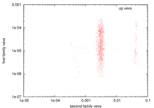
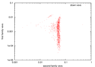
Figure 1: Values of the VEV of the scalar $SU(2)$ singlet fields in the up on the left and down sectors on the right.

$$10^{-6}~{}<~{} v_{1}^{u} ~{}<~{}10^{-4}$$

$$2\cdot 10^{-3}~{}<~{} v_{2}^{u} ~{}<~{}3\cdot 10^{-3}$$

$$10^{-4}~{}<~{} v_{1}^{d} ~{}<~{}10^{-2}$$

$$2\cdot 10^{-2}~{}<~{} v_{2}^{d} ~{}<~{}6\cdot 10^{-2}$$

in agreement with the observed mass hierarchies at the unification scale (see Table 1)

$$v_{1}^{u}:v_{2}^{u}:v_{3}^{u}=m_{u}:m_{c}:m_{t}=\lambda^{7}:\lambda^{4}:1,$$ (30)

$$v_{1}^{d}:v_{2}^{d}:v_{3}^{d}=m_{d}:m_{s}:m_{b}=\lambda^{4}:\lambda^{2}:1.$$ (31)

Relations (30) and (31) show that in quark sector the S₃ symmetry is totally broken.

The magnitude of $g_{2}^{u,d},~{}g_{L}^{u,d},~{}g_{R}^{u,d}$ and $g_{3}^{u,d}$ are related to the $t$s exponents like in eq. (26). In Fig. (2) we report the montecarlo results for the $t$s exponents given by the statistical analysis allowed after the application of the experimental constrains eq. (29).

Figure 2: $t$ exponents that parametrize the magnitude of the $g$ couplings in the general case. We have plotted the plane $(t_{L}^{d},t_{R}^{d})$, $(t_{L}^{u},t_{R}^{u})$, $(t_{3}^{u},t_{3}^{d})$ and $(t_{2}^{u},t_{2}^{d})$.

From these figures it is not difficult to obtain the following bounds for the $t$ exponents

$$\begin{array}[]{ccccccc}0<&t_{L}^{u}&<8&;&3<&t_{R}^{u}&<8,\\ 4.5<&t_{3}^{u}&<8&;&5<&t_{2}^{u}&<8.\\ \end{array}$$ (32)

$$\begin{array}[]{ccccccc}0<&t_{L}^{d}&<1&;&2.5<&t_{R}^{d}&<8,\\ 2.5<&t_{3}^{d}&<3&;&5<&t_{2}^{d}&<8.\end{array}$$ (33)

The upper bounds $t=$8 in eq. (32) and eq. (33) is the cutoff used in the montecarlo method, see eq. (28). An upper bound $t<\alpha<8$ correspond to a $g$ coupling lower bound, namely $|g|>\lambda^{\alpha}$. In the up quark sector, $g$s couplings are not bounded from below since the corresponding $t$s exponents could be large, namely in eq. (32) all the $t$s exponents can be taken equal to the cutoff used in the statistical analysis. This means that all the $g$s couplings in the up quark sector can be very small of order $\lambda^{8}$. In contrast, in the down sector the couplings $g_{L}^{d}$ and $g_{3}^{d}$ are bounded from below

$$|g_{L}^{d}|>\lambda,~{}~{}|g_{3}^{d}|>\lambda^{3},$$ (34)

while the couplings $g_{2}^{d}$ and $g_{R}^{d}$ in the down sector can be very small like in the up quark sector. Experimental data statistically prefer models where the absolute value of the $|g_{L}^{d}|$ coupling is large, see eq. (34). In particular $|g_{L}^{d}|$ can be close to one or to the maximal value allowed in the montecarlo analysis, see eq. (28) and it is slightly smaller than $g^{d}=1$. Indeed from relations (33) and (34) the $g_{3}^{d}$ coupling also has an upper bound, that is $|g_{3}^{d}|<\lambda^{2.5}\ll\lambda$. Therefore from the statistical analysis we get the following hierarchies between the $g$s couplings

$$1~{}=~{}g^{u}~{}=~{}g^{d}~{}\simeq~{}|g_{L}^{d}|~{}\gg~{}|g_{3}^{d}|~{}\gg~{}|g_{2}^{d}|,~{}|g_{R}^{d}|,~{}|g_{2}^{u}|,~{}|g_{L}^{u}|,~{}|g_{R}^{u}|,~{}|g_{3}^{u}|.$$ (35)

In Table 3 we report a numerical example of values for the $g$s coupling and for the vevs that fit good data.

up	down
$\phi^{u}_{1}/\phi^{u}_{3}=m_{u}/m_{t}$	$\phi^{d}_{1}/\phi^{d}_{3}=0.000077$
$\phi^{u}_{2}/\phi^{u}_{3}=m_{c}/m_{t}$	$\phi^{d}_{2}/\phi^{d}_{3}=0.054783$
$g=1$	$g=0.848$
$g_{L}\simeq 0$	$g_{L}=0.305~{}e^{-i~{}0.02}$
$g_{R}\simeq 0$	$g_{R}=0.002~{}e^{-i~{}0.12}$
$g_{L}\simeq 0$	$g_{L}~{}=0.009~{}e^{i~{}1.82}$

Table 3: Example of set of values of $g$ couplings and vevs that fit the data.

III.3 The CKM and the couplings $g_{L}^{d}$ and $g_{3}^{d}$

The statistical analysis results in previous section, show that in first approximation the experimental data can be fitted only with couplings $g^{u},~{}g^{d},~{}g_{L}^{d}$ and $g_{3}^{d}$ couplings ($g^{u,d}$ are fixed), besides the vevs of the scalar fields. In this section we want to study the relation between the $g_{L}^{d}$ and $g_{3}^{d}$ and the entries of the CKM mixing matrix. Accordingly we fix the values of the scalar vevs like in eq. (30) and eq. (31). From eq. (30), eq. (31) and eq. (35) we get, up to correction of order $\lambda^{8}$, the mass matrices below

$$M^{u}\simeq v_{H}^{u}\left(\begin{array}[]{ccc}\lambda^{7}&0&0\\ 0&\lambda^{4}&0\\ 0&0&1\end{array}\right)~{},~{}~{}~{}M^{d}\simeq v_{H}^{d}\left(\begin{array}[]{ccc}\lambda^{4}&g_{L}^{d}~{}\lambda^{4}+g_{3}^{d}&g_{L}~{}\lambda^{4}+g_{3}^{d}~{}\lambda^{2}\\ g_{L}^{d}~{}\lambda^{2}+g_{3}^{d}&\lambda^{2}&g_{L}^{d}~{}\lambda^{2}+g_{3}^{d}~{}\lambda^{4}\\ g_{L}^{d}+g_{3}^{d}~{}\lambda^{2}&g_{L}^{d}+g_{3}^{d}~{}\lambda^{4}&1\end{array}\right).$$ (36)

The up quark mass matrix in eq. (36) is almost diagonal and the quark mixing matrix $V_{CKM}$ is approximatively given by the unitary matrix $U_{d}$ that diagonalize on the left the down quark mass matrix eq. (36), namely $U_{d}^{\dagger}~{}M_{d}~{}M_{d}^{\dagger}~{}U_{d}=D_{d}^{2}$. We observe that in general the $g_{L}^{d}$ and $g_{3}^{d}$ are arbitrary complex variables. In order to simplify the problem, we assume $g_{L}^{d}$ and $g_{3}^{d}$ reals and the CKM complex phase $\eta$ is not fitted.

In the standard parametrization $V_{CKM}=R_{23}~{}R_{13}~{}R_{12}$ where $R_{ij}$ are rotations in the $(ij)$ plane of $\theta_{ij}$ angles, then $|V_{cb}|\approx\sin\theta_{23}$ and $|V_{ub}|\approx\sin\theta_{13}$. From mass matrices (36) we have

$$|V_{cb}|\simeq\frac{1}{\sqrt{2}}\sqrt{1+\frac{(1+2g_{L}^{2})(\lambda^{4}-1)}{\sqrt{16g_{L}^{3}\lambda^{4}+(\lambda^{4}-1)^{2}+4g_{L}^{4}(1-\lambda^{4}+\lambda^{8})}}}$$ (37)

where $g_{L}=\lambda^{t_{L}}$, so in first approximation $|V_{cb}|$ is only a function of the coupling $g_{L}^{d}$.

Figure 3: Plot of the function $|V_{cb}|=V_{cb}(t_{L})$ and $|V_{ub}|=V_{ub}(t_{3})$.

In Fig. 3 we plot the function $|V_{cb}|=V_{cb}(t_{L})$. We observe that when $t_{L}\simeq 0.5$ the corresponding $|V_{cb}|$ agree with data and $t_{L}\simeq 0.5$ is close to the value from the montecarlo, see in eq. (33).

Analogously we can use the remaining free parameter $g_{3}^{d}$ to fit the $|V_{ub}|$ as below

$$|V_{ub}|\simeq\frac{1}{\sqrt{2}}\sqrt{1+\frac{g_{3}^{2}-4g_{3}\lambda^{2}-3}{\sqrt{9+g_{3}^{4}+24g_{3}\lambda^{2}-8g_{3}^{3}+2g_{3}^{2}(10\lambda^{4}+4\lambda^{2}-1)}}}.$$ (38)

In Fig. 3 we have plotted the function $V_{ub}(t_{3})$. $|V_{ub}|$ agrees with experimental data when $t_{3}\simeq 3$, in agreement with statistical analysis. $|V_{ub}|$ is approximatively only a function of $g_{L}^{d}$ coupling. Assuming for instance $t_{L}=0.55$ and $t_{3}=3.1$ in eq. (36), we have $|V_{us}|\simeq 0.21$, $|V_{ub}|\simeq 0.004$ and $|V_{cb}|\simeq 0.043$ that agree with data.

IV Conclusions

Recently it has been proposed in Ref. Caravaglios:2005gf a model based on $E_{6}\times S_{3}$ in order to explain fermions mass and mixing hierarchies. However a full study of $S_{3}$ breaking pattern was not accomplished. We carry out such a study. In the model of Ref. Caravaglios:2005gf quark mass terms appear as higher order dimension five operators after $S_{3}$ is broken. We have showed that in such a model quark mass matrices are parametrized by five complex couplings $g^{u,d},~{}g_{2}^{u,d},~{}g_{L}^{u,d},~{}g_{R}^{u,d},~{}g_{3}^{u,d}$ and three real parameters $v_{1}^{u,d},~{}v_{2}^{u,d},~{}v_{3}^{u,d}$ that are the vevs of the scalar fields that break $S_{3}$. Even if we can assume $g^{u}=g^{d}=1$ and $v_{1}^{u}=v_{1}^{d}=1$, the number of free parameters in the model is larger than the number of experimental data then it is not possible to fit the parameters. To go forward we have used a numerical approach finding the statistically preferred textures of the mass matrices according to a goodness of fit criterion. We have found that the permutation symmetry $S_{3}$ is totally broken and vev hierarchies should be $v_{1}^{u,d}\ll v_{2}^{u,d}\ll v_{3}^{u,d}$, and data statistically prefer solutions with large $|g_{L}^{d}|$ coupling, namely slightly smaller than $g^{u}=1$, and $|g_{3}^{d}|\approx\lambda^{3}$ while the remain couplings in up and down quark textures, are negligible and are of order $\lambda^{8}$. The resulting up quark mass matrix is almost diagonal and the quarks mixing matrix is approximatively given by the down quark mass matrix that is not symmetric. The hierarchies between the yukawa couplings is

$$1~{}=~{}g^{u}~{}=~{}g^{d}~{}\simeq~{}|g_{L}^{d}|~{}\gg~{}|g_{3}^{d}|~{}\gg~{}|g_{2}^{d}|,~{}|g_{R}^{d}|,~{}|g_{2}^{u}|,~{}|g_{L}^{u}|,~{}|g_{R}^{u}|,~{}|g_{3}^{u}|.$$ (39)

Ultimately we have studied the relation between the couplings $g_{L}^{d}$, $g_{3}^{d}$ and the CKM mixing matrix. We have found that $V_{cb}$ is approximatively a function of $g_{L}^{d}$ coupling and $V_{ub}$ is approximatively a function of $g_{3}^{d}$ coupling.

The study of the breaking pattern of the $S_{3}$ symmetry in the quark sector, gives indications to go forward in the model building. In fact recently in Ref. Caravaglios:2006aq it has been studied a model that could explains quark, lepton and neutrino mixings and masses, making use of the montecarlo statistical analysis results reported in this paper. In particular in the model of Ref. Caravaglios:2006aq are explained the hierarchies in eq. (39) between the $g$s Yukawa couplings. In third quantization models it is possible to extend the concept of family to the gauge bosons through the semidirect product of a gauge group $G$, with the group of the permutation of $n$ objects, namely $G^{n}>{}\triangleleft S_{n}$. In Ref. Caravaglios:2006aq it has been proposed a $E_{6}^{4}>{}\triangleleft S_{4}$ model where $E_{6}$ is the grand unified gauge group and $S_{4}$ is the permutation symmetry of four objects. It is showed that embedding $S_{3}\subset S_{4}$ it is possible to better explain neutrino oscillation, while $E_{6}^{4}$ could be useful in order to understand the hierarchies between the $g$s couplings reported in eq. (39). It is presented a possible breaking pattern of $E_{6}^{4}>{}\triangleleft S_{4}$ in agreement with our montecarlo results. In the following we report such a breaking pattern.

Assume that the starting group $E_{6}^{4}>{}\triangleleft S_{4}$ is broken into the group $G_{1}=(SM\times U(1)_{r}\times U(1)_{t})^{4}>{}\triangleleft S_{4}$ where $U(1)_{r}$ and $U(1)_{t}$ are defined as $E_{6}\supset SO(10)\times U(1)_{t}\supset SU(5)\times U(1)_{r}\times U(1)_{t}$ and $SM$ is the Standard Model gauge group. At some scale $M_{1}$ the group $G_{1}$ breaks into the group $G_{2}=(SM\times U(1)_{r}\times U(1)_{t})^{3}>{}\triangleleft~{}S_{3}$. It is easy to see that the only operators compatible with $G_{2}$ are

$$g~{}\bar{d}_{L}^{i}d_{R}^{i}H\phi_{i}.$$

The coupling $g$ will be of order of magnitude $g\simeq M_{1}/\Lambda$ where $\Lambda$ is the characteristic scale of $E_{6}^{4}>{}\triangleleft S_{4}$. At another scale $M_{2}<M_{1}$ the group $G_{2}$ breaks into $G_{3}=(SM\times U(1)_{\mathrm{down}})^{3}>{}\triangleleft S_{3}$ where $U(1)_{\mathrm{down}}$ is defined as the linear combination of $U(1)_{r}$ and $U(1)_{t}$ so that right-handed down quarks do not carry $U(1)_{\mathrm{down}}$ charge. At this scale also the operators

$$\sum_{i,j}g_{L}~{}\bar{d}_{L}^{i}d_{R}^{j}H^{i}\phi_{i}$$

are allowed and $g_{L}\simeq M_{2}/\Lambda$. If $M_{1}\sim M_{2}$ it is possible to explain the relation $g\simeq g_{L}$ in eq. (39). At the scale $M_{2}$ the operators proportional to $g_{2}^{d}$, $g_{3}^{d}$ and $g_{R}^{d}$ are not allowed. They only appear after the breaking of $U(1)_{\mathrm{down}}$ at some scale $M_{3}<M_{2}$. If $M_{2}\gg M_{3}$ we can explain the hierarchy $g_{L}^{d}\gg g_{3}^{d},~{}g_{R}^{d},~{}g_{2}^{d}$.

References

• (1) F. Caravaglios and S. Morisi, arXiv:hep-ph/0510321.
• (2) F. Caravaglios, arXiv:hep-ph/0211183; F. Caravaglios, arXiv:hep-ph/0211129; V. A. Rubakov, Phys. Lett. B 214, 503 (1988); M. McGuigan, Phys. Rev. D 38, 3031 (1988); S. B. Giddings and A. Strominger, Nucl. Phys. B 321, 481 (1989).
• (3) P. F. Harrison, D. H. Perkins and W. G. Scott, Phys. Lett. B 530, 167 (2002) [arXiv:hep-ph/0202074]; K. S. Babu, E. Ma and J. W. F. Valle, Phys. Lett.  B 552, 207 (2003) [arXiv:hep-ph/0206292]; G. Altarelli and F. Feruglio, Nucl. Phys.  B 741, 215 (2006) [arXiv:hep-ph/0512103]; W. Grimus and L. Lavoura, JHEP 0508, 013 (2005) [arXiv:hep-ph/0504153].
• (4) H. Fritzsch and Z. z. Xing, Prog. Part. Nucl. Phys.  45, 1 (2000) [arXiv:hep-ph/9912358]; G. Altarelli and F. Feruglio, New J. Phys.  6, 106 (2004) [arXiv:hep-ph/0405048]; C. H. Albright and M. C. Chen, Phys. Rev.  D 74, 113006 (2006) [arXiv:hep-ph/0608137]; G. Altarelli, In the Proceedings of IPM School and Conference on Lepton and Hadron Physics (IPM-LHP06), Tehran, Iran, 15-20 May 2006, pp 0001 [arXiv:hep-ph/0610164].
• (5) G. L. Fogli, E. Lisi, A. Marrone and A. Palazzo, Prog. Part. Nucl. Phys.  57, 742 (2006) [arXiv:hep-ph/0506083]; M. Maltoni, T. Schwetz, M. A. Tortola and J. W. F. Valle, New J. Phys.  6, 122 (2004) [arXiv:hep-ph/0405172]; J. N. Bahcall and C. Pena-Garay, JHEP 0311, 004 (2003) [arXiv:hep-ph/0305159].
• (6) J. Charles et al. [CKMfitter Group], Eur. Phys. J.  C 41, 1 (2005) [arXiv:hep-ph/0406184]; M.Ciuchini et al., JHEP 0107(2001)013.
• (7) F. Caravaglios, P. Roudeau and A. Stocchi, Nucl. Phys. B 633, 193 (2002) [arXiv:hep-ph/0202055].
• (8) E. Ma, New J. Phys.  6, 104 (2004);
• (9) J. Kubo, A. Mondragon, M. Mondragon and E. Rodriguez-Jauregui, Prog. Theor. Phys.  109, 795 (2003) [Erratum-ibid.  114, 287 (2005)] [arXiv:hep-ph/0302196]; J. Kubo, A. Mondragon, M. Mondragon, E. Rodriguez-Jauregui, O. Felix-Beltran and E. Peinado, J. Phys. Conf. Ser.  18 (2005) 380; O. Felix, A. Mondragon, M. Mondragon and E. Peinado, arXiv:hep-ph/0610061.
• (10) C. R. Das and M. K. Parida, Eur. Phys. J. C 20, 121 (2001) [arXiv:hep-ph/0010004].
• (11) F. Caravaglios and S. Morisi, arXiv:hep-ph/0611078.