Thermodynamics of QCD-inspired theories

Andersen et al., (2004b, a); Warringa, (2003, 2004); Warringa et al., (2005); Warringa, (2005); Andersen et al., (2006)

promotor:	prof.dr. P.J.G. Mulders
copromotor:	dr. D. Boer

This thesis is based on the following publications

• Jens O. Andersen, Daniel Boer and Harmen J. Warringa, Thermodynamics of the O(N) nonlinear sigma model in (1+1)-dimensions, Phys. Rev. D69, 076006 (2004), hep-ph/0309091.

• Jens O. Andersen, Daniel Boer and Harmen J. Warringa, The effect of quantum instantons on the thermodynamics of the $\mathbb{C}P^{N-1}$ model, hep-th/0602082.

• Jens O. Andersen, Daniel Boer and Harmen J. Warringa, Thermodynamics of O(N) sigma models: 1/N corrections, Phys. Rev. D70, 116007 (2004), hep-ph/0408033.

• Harmen J. Warringa, Daniel Boer and Jens O. Andersen, Color superconductivity vs. pseudoscalar condensation in a three-flavor NJL model, Phys. Rev. D72, 014015 (2005), hep-ph/0504177.

• Harmen J. Warringa, Heating the O(N) nonlinear sigma model, in Proceedings of the 43rd Cracow school of theoretical physics, Acta Phys. Polon. B34, 5857 (2003), hep-ph/0309277.

• Harmen J. Warringa, Thermodynamics of the 1+1-dimensional nonlinear sigma model through next-to-leading order in 1/N, in Proceedings of the SEWM2004 meeting, World Scientific (2005), hep-ph/0408257.

• Harmen J. Warringa, Phase diagrams of the NJL model with color superconductivity and pseudoscalar condensation, to appear in proceedings of the XQCD’05 workshop, hep-ph/0512226.

Chapter 1 Introduction

What happens to matter when you squeeze it further and further? And what if it will be heated more and more? Liquid water for example will turn at some point into a different phase called steam when it is heated. If instead the density is increased at room temperature by applying an external pressure, water will subsequently turn into different types of ice, called ice VI, ice VII, etc. Such phase transitions are not specific for water, but they can take place in any interacting substance, like for example hadronic matter.

Hadronic matter is matter built out of quarks and gluons. The neutron for instance is a form of hadronic matter, it is a bound state of two down-quarks, one up-quark and gluons which keep the quarks together. Imagine a hypothetical situation in which one has lots of these neutrons in a box. Then increase the temperature. What will happen? At some point the kinetic energy of the quarks which build up the neutron will become larger than the energy that is gained by confining the quarks inside the neutron. At this point the neutrons will cease to exist. The matter in the box is now in a new phase, which is called the quark gluon plasma. An order of magnitude estimate of this transition temperature can easily be made. Classically the kinetic energy of a quark at temperature $T$ is about $3T/2$. Since the masses of the quarks are much smaller than the neutron mass, the mass of the neutron is almost completely due to confining energy. So the confining energy per quark is about $m_{N}/3\approx 300\;\mathrm{MeV}$. This implies that the transition temperature $T_{c}$ to the quark gluon plasma should be around $T_{c}=200\;\mathrm{MeV}$, which is very hot (actually it is about $10^{5}$ times the temperature of the solar core). In nature these temperatures were achieved in the early universe and are possible in relativistic heavy ion collisions for extremely short periods of time.

Now start again from scratch at low temperatures and squeeze the box further and further. At some point the neutrons will start to overlap and at even higher densities they will cease to exist as separate entities. Around this point it is expected that quarks will form Cooper pairs. The matter will transform into a so-called color-superconducting state. An order of magnitude estimate shows that this will occur around densities of about $m_{N}/V_{N}\approx 160\;\mathrm{MeV}\cdot\mathrm{fm}^{-3}\approx 3\times 10^{17}\;\mathrm{kg}\cdot\mathrm{m}^{-3}$. This density is quite large, and takes only place in extremely dense objects like for example neutron stars.

The theory which describes the interactions between the quarks mediated by gluons is called quantum chromodynamics (QCD) and is treated in more detail in the following section. Using QCD one could in principle predict the behavior of matter under these extreme circumstances by calculating its equation of state (that is the relation between its pressure and energy density) and its phase diagram, which are discussed in Secs. 1.2 and 1.3 respectively. The situations in which these extreme circumstances are realized in nature are reviewed in Sec. 1.4. Since it turns out that QCD is very complicated at the energy scales around the phase transition, this thesis will deal with models inspired by QCD to describe matter at high temperatures and densities, as will be discussed in more detail in Secs. 1.5 and 1.6. A more extensive review on QCD at high temperatures and densities can be found in for example Meyer-Ortmanns, (1996), Rajagopal and Wilczek, (2000) and Rischke, (2004).

1.1 Quantum chromodynamics

Quantum chromodynamics (QCD) is a non-Abelian $\mathrm{SU}(3)$ gauge field theory which describes the interactions between the quarks. It is a generalization of Maxwells theory of electromagnetism. Like the electrons, quarks carry a charge, called color. Unlike the photons in electromagnetism, the gluons, which are the force carriers of QCD carry a color charge as well. As a result the gluons interact with themselves and with quarks. Due to the $\mathrm{SU}(3)$ gauge symmetry QCD has three different color charges, named red, blue and green. Together with the electroweak theory, QCD is one of the building blocks of the Standard Model of elementary particle physics. QCD is defined by the following Lagrangian density

$$\begin{split}\mathcal{L}&=\bar{\psi}\left(i\gamma^{\mu}\mathcal{D}_{\mu}-m_{0}+\mu\gamma_{0}\right)\psi-\frac{1}{4}F^{\mu\nu}_{a}F_{\mu\nu}^{a}\;,\\ \mathcal{D}_{\mu}&=\partial_{\mu}-igA^{a}_{\mu}T_{a}\;,\;\;\;\;\;\;\;F_{\mu\nu}^{a}=\partial_{\mu}A^{a}_{\nu}-\partial_{\nu}A^{a}_{\mu}+gf^{a}_{bc}A^{b}_{\mu}A^{c}_{\nu}\;,\end{split}$$ (1.1)

where $g$ is the QCD coupling constant, $T_{a}$ is a hermitian generator of $\mathrm{SU}(3)$ and $f^{a}_{bc}$ denotes its corresponding structure constant. The matrices $m_{0}$ and $\mu$ are diagonal and contain the current quark masses and the quark chemical potentials respectively. There are six different quark flavors. The up, down and strange quark are relatively light, while the charm, bottom and top quark are heavy. Since the masses of the heavy quarks are so much larger than the estimated transition temperature of about 200 MeV, these quarks will play a minor role at these energies and will therefore be neglected in this thesis. The discussion in this thesis will mainly deal with two ($N_{f}=2$) and three-flavor ($N_{f}=3$) situations.

The chemical potentials are necessary to describe a system at finite density. The baryon chemical potential $\mu_{B}=\mu_{u}+\mu_{d}+\mu_{s}$ for example, is basically the energy it takes to add one additional baryon to the system. Temperature is introduced by considering a Euclidean space in which the $x_{0}$ direction is made periodic (for bosons) or antiperiodic (for fermions) with periodicity $1/T$. Field theory at finite temperature and densities is discussed in more detail in Chapter 2.

QCD has different symmetries which are reflected in the hadron spectrum as a consequence. First of all it is invariant under local $\mathrm{SU}(3)$ transformations. This implies for example that red up quarks are as heavy as blue up ones. In addition, in absence of quark masses and chemical potentials, QCD has a global chiral $\mathrm{SU}(N_{f})_{L}\times\mathrm{SU}(N_{f})_{R}$ symmetry. Moreover it has a global $\mathrm{U}(1)_{B}$ symmetry related to baryon number conservation and a global $\mathrm{U}(1)_{A}$ (axial) symmetry. At low temperatures and chemical potentials it turns out that the chiral symmetry is spontaneously broken down to $\mathrm{SU}(N_{f})_{V}$ giving rise to $N_{f}^{2}-1$ massless pseudoscalar Goldstone modes. For $N_{f}=2$ these are the three pions, for $N_{f}=3$ also the four kaons and the $\eta$ particle are among the pseudoscalar Goldstone modes. If chiral symmetry is broken the $\langle\bar{u}u\rangle$, $\langle\bar{d}d\rangle$, and $\langle\bar{s}s\rangle$ condensates obtain a vacuum expectation value.

However, in reality the quarks have a small mass. Therefore chiral symmetry is only an approximate symmetry, as a result the pions, the kaons and the $\eta$ particle become massive. This remaining (approximate) $\mathrm{SU}(N_{f})_{V}$ symmetry is the reason why the constituent quark model of Gell-Mann works as well as it does. Particles are eigenstates of the QCD Hamiltonian which due to the symmetry commutes with $\mathrm{SU}(N_{f})_{V}$. Hence the particles can be classified by the representations of $\mathrm{SU}(N_{f})_{V}$. At high temperatures and/or densities the chiral symmetry is approximately restored, giving rise to a phase transition. Although the $\mathrm{U}(1)_{A}$ symmetry is broken due to nonzero quark masses as well, it also has another reason of breakdown. The non-trivial topological vacuum structure of QCD due to instantons is causing $\mathrm{U}(1)$ axial symmetry breaking too, which explains the relatively high mass of the $\eta$ meson (’t Hooft, , 1976).

One of the mysteries in QCD is confinement. It turns out experimentally that hadrons, which are bound states of quarks, carry no color. Colored objects, like freely moving quarks, do not occur in nature at low energies. In numerical computations (lattice QCD) it is confirmed that QCD has this confinement property. But a detailed understanding of the confinement mechanism is still lacking. At high temperatures and/or chemical potentials it is expected that matter will be in a deconfined phase, which means that in that situation quarks are liberated from the hadrons. Whether the deconfinement phase transition for light quarks coincides with the chiral symmetry restoration transition is an important issue which has not yet been resolved.

QCD is asymptotically free, this implies that the effective coupling of quarks to gluons becomes smaller at high energies. So at high energy scales, larger than about $1\;\mathrm{GeV}$, QCD is a theory of weakly interacting quarks and gluons. Due to the small coupling constant it is possible to perform calculations in this regime using perturbation theory. But, at lower energies QCD becomes strongly coupled and perturbation theory breaks down. The order of magnitude estimate of the transition temperature $T_{c}\approx 200\;\mathrm{MeV}$ from the first paragraph tell us that QCD is likely to be strongly coupled around the phase transition. Hence it is expected that perturbation theory will fail to describe QCD near $T_{c}$. This will be illustrated next by comparing perturbative and lattice calculations of the QCD pressure.

1.2 QCD equation of state

Two important macroscopic thermodynamical quantities are the pressure $\mathcal{P}$ and the energy density $\mathcal{E}$ of QCD. The relation between $\mathcal{E}$ and $\mathcal{P}$ is called the equation of state and determines for example the behavior of matter created in a relativistic heavy ion collision, the properties of a (neutron) star and the evolution of the early stage of the universe shortly after the big bang, see Sec. 1.4. Due to asymptotic freedom, QCD describes a gas of weakly interacting quarks and gluons in the limit of very high temperature. In that case the coupling constant is small, and hence perturbation theory should be applicable. However as will be shown next perturbation theory does not work for the temperatures of in the neighborhood of $T_{c}$.

Perturbative calculations

The results of the perturbative calculation of the pure glue (which means no quarks) QCD pressure compared to numerical calculations (lattice QCD) are displayed in Fig. 1.1 up to order $\alpha^{5/2}=(g^{2}/4\pi)^{5/2}$. It can be seen in the figure that for temperatures in the neighborhood of the transition temperature $T_{c}$, the results are varying a lot upon inclusion of higher order corrections. This implies that the perturbative expansion breaks down, even for very high temperatures of around $1000T_{c}$. However, by reorganizing the perturbative series using resummation methods (Andersen et al., , 1999, 2002) and self-consistent approaches (Blaizot et al., , 1999) based on hard thermal loops (Braaten and Pisarski, , 1990) it is possible to obtain reliable results for $T\gtrapprox 3T_{c}$. In perturbation theory it is impossible to calculate the order $g^{6}$ contribution because an infinite number of diagrams are contributing in this order and cannot be resummed as was argued by Linde, (1980).

It is possible to perform perturbation theory for finite chemical potentials as well, but it again fails for densities where the phase transition occurs. Also this perturbation series can be improved by applying the so-called hard dense loop resummation method (Andersen and Strickland, , 2002).

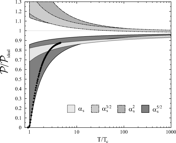
Figure 1.1: Perturbative results (indicated by their orders) and lattice results of (Boyd et al., , 1996) (indicated with black diamonds) of the pure glue QCD pressure normalized to the ideal gas value, as a function of $T/T_{c}$. The shaded regions arise due to varying the $\overline{MS}$ renormalization scale between $\pi T$ and $4\pi T$ and are hence an indication of the error that is inherent to truncating the perturbative series. The order $\alpha$ calculation was performed by Shuryak, (1978), $\alpha^{3/2}$ by Kapusta, (1979), $\alpha^{3/2}\log\alpha$ by Toimela, (1983), $\alpha^{2}$ by Arnold and Zhai, (1995), $\alpha^{5/2}$ by Zhai and Kastening, (1995) and Braaten and Nieto, (1996) and order $\alpha^{3}\log\alpha$ (not shown in figure) by Kajantie et al., (2003). This figure is adapted from Andersen et al., (2002).

Lattice calculations

The best known method to obtain the QCD thermodynamical quantities from first principles near the phase transition temperature is by lattice calculations. In these calculations, space-time is discretized and replaced by a lattice of a finite size. The fermion fields live on the vertices of this lattice, the gauge fields are replaced by links connecting the different vertices. All thermodynamical quantities can be obtained by numerically calculating the partition function (discussed in Chapter 2). This requires integration over the fermion fields and links. Since this results in a huge number of integrations, typical lattice sizes are taken to be rather small, in the order of ten points for each dimension. Due to this modest lattice sizes, the particles with low mass (like the pion), which can propagate over longer distances are not very well described. The integrations in lattice calculations are performed statistically, using importance sampling Monte-Carlo methods. This works fine for QCD at zero chemical potential. But at finite baryon chemical potential, the contribution from the fermions, the so-called fermionic determinant, becomes imaginary (see also Chapter 7). As a result, the integrand of the partition function becomes oscillatory, which hampers the importance sampling methods. This complication is called the fermion sign problem. Small baryon chemical potentials are, however, accessible by making a Taylor expansion around $\mu_{B}=0$ (Allton et al., , 2002; Fodor and Katz, , 2002; de Forcrand and Philipsen, , 2002; D’Elia and Lombardo, , 2003).

In Fig. 1.2 the lattice results of the pressure of QCD for different numbers of quark flavors are displayed as a function of $T$ for $\mu=0$. Here $T_{c}\approx\;170\;\mathrm{MeV}$. From the figure it can be seen that the QCD pressure rises quickly after passing the transition point. This may be an indication that many new degrees of freedom are formed, just what one would expect if the quarks become deconfined from the hadrons. The figure shows that even around $4T_{c}$ the pressure is still far away from that of a freely interacting gas of quarks and gluons $\mathcal{P}=\mathcal{P}_{\mathrm{SB}}$. While the lattice gives reliable results for $T>T_{c}$, the data at $T<T_{c}$ can not be trusted. This is because the pion, the lightest particle of QCD, which is expected to dominate the pressure of QCD at low temperatures is still far too heavy on the lattice.

Figure 1.2: Lattice calculation by Karsch et al., (2000) of the pure glue and full QCD pressure (for 2 light quark flavors, 2 light & 1 heavy flavor and 3 light flavors), normalized to $T^{4}$, as a function of $T$. The arrows indicate the limit of the pressures when $T\rightarrow\infty$ and are calculated in Sec. 2.4. This figure is adapted from Karsch, (2002).

For $T>T_{c}$ the lattice data for the QCD pressure can be fitted to quasiparticle models (Peshier et al., , 1996; Levai and Heinz, , 1998; Schneider and Weise, , 2001). The results of these fits can be extended to finite chemical potential (Rebhan and Romatschke, , 2003; Thaler et al., , 2004). In this way the equation of state of QCD at finite chemical potential for $T>T_{c}$ can be predicted.

It is generally believed that the lattice calculations of the pressure are reliable for temperatures around $T_{c}$ and higher. The results at high temperatures can be predicted by hard-thermal-loop resummation methods. At low temperatures lattice QCD is still unreliable due to the unrealistically large pion mass. In order to predict the pressure of QCD at low temperatures one can use a low-energy effective theory in order to describe the hadron gas phase as is done in this thesis in Chapter 6 and will be discussed in more detail in Sec 1.5.

1.3 QCD phase diagram

By considering the behavior of order parameters (parameters which vanish in one phase and are non-vanishing in another) one can determine a phase diagram. One typically distinguishes between two different types of phase transitions, a first order phase transition in which the order parameter changes discontinuously and a second order phase transition in which the derivative of the order parameter changes discontinuously. Higher order phase transitions are also possible, but are often called second order transitions as well. In addition, cross-over transitions in which the order parameter changes smoothly can occur. The different possibilities are displayed in Fig. 7.1.

In the limit of zero quark masses the chiral condensates, $\left<\bar{u}u\right>$, $\langle\bar{d}d\rangle$ and $\left<\bar{s}s\right>$ are order parameters for the breaking of chiral symmetry. In Sec. 1.1 it was mentioned that the chiral symmetry is already explicitly broken in the QCD Lagrangian density due to the non-zero quark masses. In that case the chiral condensates are only approximate order parameters. The order parameter for the confinement/deconfinement transition in the limit of infinitely heavy quarks is the trace of the so-called Polyakov loop. For finite quark masses no order parameter for this transition is known, see for example Weiss, (1993).

Figure 1.3: Schematic structure of the current understanding of the phase diagram of QCD. First order phase transitions are indicated with a solid line, second order with a dashed line and a cross-over with a dotted line. In the diagram the cooling trajectory of the early universe and of matter produced in heavy ion collisions is sketched. It is also roughly indicated in which phase the matter inside neutron stars can be.

In Fig. 1.3 the current understanding of the QCD phase diagram is displayed schematically. As was discussed in the previous section, only results for zero and small baryon chemical potential can be obtained from lattice QCD. Lattice calculations find a cross-over transition at $T_{c}=170\;\mathrm{MeV}$. The rest of the phase diagram is not yet obtained from first principles QCD but can be estimated by means of effective models like the NJL model studied in Chapter 7. However, the phases with temperatures and densities much higher than the densities and temperatures where the phase transition takes place are accessible by hard-thermal loop and hard-dense loop resummation techniques as was discussed in the previous section. The NJL phase diagram as a function of $\mu_{B}$ and $T$ is displayed in Fig. 7.4.

As mentioned before, finite chemical potentials are needed to describe a system at finite density. However, it is important to keep in mind that the relation between chemical potential and number density is not linear. Especially at a first order phase transition, a single value of a chemical potential can correspond to a whole range of densities, as is illustrated for the NJL model in Fig 7.2. In this case one also speaks of a mixed phase, two phases can occur together. The world we live in is an example of a mixed phase of nuclear matter and vacuum. One should be aware that the real phase diagram of matter is not just the QCD phase diagram. To obtain the complete phase diagram of matter, one should also take into account the electromagnetic and weak interactions.

The best known point in the QCD phase diagram, is the transition from the vacuum to the nuclear matter phase, there is a first order phase transition at $\mu_{B}=922\;\mathrm{MeV}$, see also Halasz et al., (1998).

It is illustrated in Fig. 1.3 that matter at low chemical potentials and temperatures matter is in a confined phase in which chiral symmetry is broken as well. If the temperature is increased, matter goes according to the current understanding via a cross-over transition to the deconfined and chirally symmetric phase at low chemical potentials, and via a first-order transition at higher chemical potentials. This deconfined phase is called the quark-gluon plasma. The point in which the first-order transition goes over to a cross-over is called the critical endpoint. It still is uncertain where this critical endpoint lies exactly in the phase diagram. At low temperatures and high chemical potentials due to an attractive interaction, quarks can form Cooper pairs just like electrons in ordinary superconductivity. This phenomenon will be discussed in more detail in Chapter 7.

The phase diagram in Fig. 1.3 is displayed as a function of baryon chemical potential and temperature. Of course it is interesting to investigate other phase diagrams as well, for example as a function of the quark masses, as is discussed in Laermann and Philipsen, (2003). In Chapter 7 phase diagrams of the NJL model will be investigated for unequal chemical potentials and temperature. In that case a new possibility appears which is not present in Fig. 1.3, namely quarks can form pseudoscalar condensates, like the pion condensate $\langle\bar{u}i\gamma_{5}d\rangle$.

In Fig. 1.3 it is also indicated which part of the phase diagram can be investigated using relativistic heavy ion collisions, which kind of matter neutrons stars are presumably made of, and through which phases the early universe went shortly after the big bang. In the following section these three situations will be examined in somewhat more detail.

1.4 Matter under extreme conditions

Typical situations in which temperatures and densities could be high enough for deconfinement to occur, are the universe just after the big bang, during heavy ion collisions and inside very compact neutron stars. In this section a short overview of these situations is given. More extensive discussions can be found in for example Ellis, (2005) (the big bang in relation to heavy ion collisions), Gyulassy and McLerran, (2005) (heavy ion collisions) and Weber, (2005) (neutron stars).

The big bang

In one of the earliest stages of the universe, about $10^{-6}$ seconds after the big bang, the universe was still so hot that the matter inside was in the deconfined phase, i.e. the quark gluon plasma. Since at that time the particles and antiparticles had not annihilated yet, the baryon chemical potential was very small. As is indicated in Fig. 1.3 when the universe cooled, it probably went through a cross-over transition to the confined phase. Since a cross-over transition is smooth, it is unlikely that the expansion of the universe was modified substantially during this transition.

To describe the evolution of the universe one has to use an equation of state. Most often a simple equation of state is used, $\mathcal{P}=\mathcal{E}/3$ for the radiation dominated era at early times, and $\mathcal{P}=0$ for the matter dominated era which occured later. The description can be made more realistic by using the QCD equation of state.

Relativistic heavy ion collisions

The behavior of matter under extreme circumstances can be studied experimentally using heavy ion collisions. Such experiments have been performed at the Super-Proton-Synchrotron (SPS) at CERN and are being performed at the Relativistic Heavy Ion Collider (RHIC) at BNL. Currently new accelerators which, among other things, will be used for relativistic heavy ion collision studies are being build at CERN (the Large Hadron Collider (LHC)), and at GSI (Schwerionen-Synchrotron (SIS 200)).

In a typical relativistic heavy ion collision two incoming heavy nuclei (for example gold with 197 nucleons) collide at relativistic energies. At RHIC these energies are up to 200 GeV per nucleon. During the collision a large fraction of the kinetic energy is converted into particles. Therefore statistical methods can be used to describe the system. High temperatures and energy densities are achieved during these collisions. The baryon chemical potential remains low in a heavy ion collision. The reason for this is that due to the large production of particle antiparticle pairs, the initial dominance of particles over antiparticles is washed out. Since SIS 200 will operate at a lower energy than RHIC and LHC, a higher baryon chemical potential can be achieved. However as a result the final temperature will be lower, which could make it more difficult to probe the phase transition.

At RHIC it seems that the produced matter quickly achieves thermal equilibrium. After that moment, relativistic hydrodynamics can describe the evolution using the QCD equation of state. This indicates that the matter created during the collisions at RHIC has a very low viscosity, possibly the most perfect fluid ever made.

That a statistical description to model heavy ion collisions works, is illustrated in Fig. 1.4. In that figure, a prediction of the ratio of particle yields is compared to the experimental data of the four different experiments at RHIC (Braun-Munzinger et al., , 2001). The statistical model only has two fit parameters, $T\approx 174\;\mathrm{MeV}$ and $\mu_{B}\approx 46\;\mathrm{MeV}$. It can also be seen from the figure that the baryon chemical potential is not that big compared to the temperature, because the ratio between particles and antiparticles of the same hadronic species are close to unity.

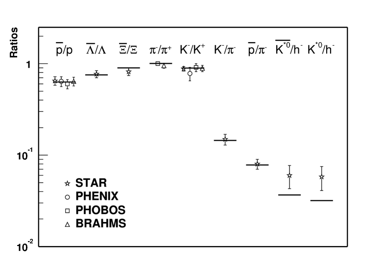
Figure 1.4: Prediction of ratios of produced particles for gold-gold collisions at $\sqrt{s}=130\;\mathrm{GeV}$ by a statistical model compared to results of the four different experiments at RHIC. This figure is adapted from Braun-Munzinger et al., (2001).

The main objective of these heavy ion collision experiments is to produce the quark gluon plasma and measure its properties. One of the clearest signals for the creation of a very dense and hot state of matter comes from the suppression of back-to-back correlations between two high transverse-momentum jets. In a collision at low energy densities, such a jet should be correlated with a jet produced in the opposite direction due to momentum conservation. This is indeed observed in heavy ion collision experiments. However, at energies of 200 GeV per nucleon in central gold-gold collisions at RHIC, this correlation has suddenly disappeared. This indicates that the momentum of the opposite jet is absorbed in a very hot and dense medium, probably the quark-gluon plasma.

Using heavy ion collisions it is difficult to reach high chemical potentials, so in order to investigate that situation one has to look to extremely compact objects like neutron stars.

Neutron stars

If the mass of a star is larger than about ten times the solar mass, the fusion process can continue until an iron-nickel core is formed. Then fusion will stop since iron is the nucleus which has the lowest binding energy per nucleon. As a result the temperature of the core will drop, hence the pressure will go down. Then the gravitational interactions cause the core to collapse until nuclear densities are reached. At this point the collapse stops because it takes a lot of energy to squeeze the core further. This creates a shock wave which as a result emits all of the matter from the shells surrounding the collapsed core. This event is called a supernova explosion. The remaining core cools down and becomes a neutron star or at even higher densities a black hole. Typical densities could be so high that the core of a neutron star is a color superconductor. Using the QCD equation of state at high-densities, the so-called Tolman-Oppenheimer-Volkov relation can be applied to calculate the mass as a function of the radius of a neutron star, see for example Fraga et al., (2001) and Andersen and Strickland, (2002). These mass-radius relationships can be compared to observations. However, until now there has not yet been discovered a neutron star from which one is certain that the inner core is so dense that it must be in a color superconducting phase.

1.5 QCD inspired theories

As was argued in the previous sections, due to the nonperturbative nature of QCD near the phase transition, it is not known how to obtain for example the order of the phase transition, the equation of state and the phase diagram using analytical methods from first principles QCD for all temperatures and chemical potentials. Also the confinement/deconfinement mechanism is not understood analytically. However, toy models (models which share features with QCD) and low-energy effective theories (theories which describe QCD in the non-perturbative regime) can be studied to learn about certain aspects to be addressed below.

Toy models

Toy models for QCD are models which have features in common with QCD. One can study these models in order to learn about nonperturbative methods and phenomena like for example the behavior of thermodynamical quantities, the generation of a mass gap, confinement and the importance of topological configurations like instantons. In this thesis two of these toy models are studied, the $\mathrm{O}(N)$ nonlinear sigma model in $1+1$ dimensions in Chapter 3 and the $\mathbb{C}P^{N-1}$ model in $1+1$ dimensions in Chapter 4. The nonlinear sigma model is a real scalar field theory which like QCD is asymptotically free and has a dynamically generated mass gap. The $\mathbb{C}P^{N-1}$ model contains complex scalar fields and $\mathrm{U}(1)$ gauge fields. This model is also asymptotically free, has a dynamically generated mass gap, contains instanton configurations and has the confinement property. In these two models it is possible to expand in the number of fields $N$. This expansion is called the large-$N$ approximation and is a method which can give insight in the nonperturbative behavior of these theories. This method will be used throughout this thesis and is discussed in more detail in Chapter 3. In this thesis the pressure for both models is calculated to next-to-leading order in $1/N$. In this way it is possible to check the validity of the $1/N$ expansion and to investigate the effects of instantons on the thermodynamical quantities in the $\mathbb{C}P^{N-1}$ model.

Low-energy effective theories

Low-energy effective theories describe QCD in the non-perturbative regime where perturbation theory is no longer applicable. The simplest examples of such an effective theory are the $\mathrm{O}(4)$ linear and nonlinear sigma model in $3+1$ dimensions. The $\mathrm{O}(4)$ symmetry (which is locally isomorphic to the chiral $\mathrm{SU}(2)_{L}\times\mathrm{SU}(2)_{R}$ symmetry of the two-flavor QCD Lagrangian) of these models is spontaneously broken to $\mathrm{O}(3)$ (which is isomorphic to the remaining chiral $\mathrm{SU}(2)_{V}$ symmetry of the QCD vacuum state). Since these models have the same symmetry breaking pattern as two-flavor QCD, they serve as a low-energy effective theory for 2-flavor QCD in which only the pion and the sigma meson can occur. Moreover for the same reason, the phase transition of the $\mathrm{O}(4)$ (non)linear sigma model falls in the same universality class as the 2-flavor QCD chiral phase transition. This allows one to study the order of the phase transition and critical exponents of QCD using the $\mathrm{O}(4)$ (non)linear sigma model. In this thesis the pressure of these models is calculated to next-to-leading order in $1/N$ in Chapter 6. In this way a prediction for the pressure of QCD at temperatures below $T_{c}$ is made, where the lattice calculations are not reliable.

Another effective theory studied in Chapter 7 of this thesis, is the Nambu–Jona-Lasinio (NJL) model. In this model the gluon exchange between the quarks is replaced by a 4-point quark interaction. As a result some features of QCD like confinement and asymptotic freedom are lost. However, low-energy properties like the meson masses are described very well using this model. Furthermore this model has the same pattern of chiral symmetry breaking as QCD. Therefore, it is expected that the NJL model gives a realistic qualitative description of the QCD phase diagram for low temperatures and chemical potentials. In Chapter 7 phase diagrams with different up, down and strange quark chemical potentials are calculated, in order to study the competition between phases in which color superconductivity is possible and in phases where the pions or kaons condense.

1.6 Overview of this thesis

To summarize, the thermodynamics of QCD inspired theories is studied in this thesis. In Chapter 2 a short introduction to finite density and temperature field theory is given. Particular emphasis is put on the analytic and numerical calculation of a combination of a sum and an integral, which will be required frequently throughout this thesis. In Chapter 3 the effective potential is derived from which by minimization one can derive the thermodynamical quantities like the pressure and determine the phase diagram. Almost all calculations in this thesis are based on evaluating this effective potential. Moreover, Chapter 3 discusses the $1/N$ approximation which can give insight into non-perturbative physics. This is also a basic ingredient for all the calculations performed in this thesis. The thermodynamics of the $\mathrm{O}(N)$ nonlinear sigma model in $1+1$ dimensions is studied in Chapter 4. In Chapter 5, the effect of quantum instantons on the thermodynamical quantities is investigated using the $\mathbb{C}P^{N-1}$ model in $1+1$ dimensions. Chapter 6 is devoted to the study of the thermodynamics of the $\mathrm{O}(N)$ linear and nonlinear sigma model in $3+1$ dimensions, which can be used to predict the pressure of QCD at low temperatures. The NJL model and its phase diagrams are discussed in Chapter 7.

1.7 Notations

Several notations are used throughout this thesis. These will be summarized here.

• Euclidean momentum vectors are denoted by a capital letter, that is $P=(p_{0},\vec{p}\,)$. The length of a momentum vector $\vec{p}$ is denoted as $p=|\vec{p}\,|$.

• The integral over Euclidean momenta, the bosonic sum-integral and the fermionic sum-integral are respectively defined as

  $$\int_{P}\equiv\int\frac{\mathrm{d}^{d+1}P}{(2\pi)^{d+1}}\;,\;\;\;\;\hbox{$\sum$}\!\!\!\!\!\!\int_{P}\equiv T\!\!\!\!\sum_{p_{0}=2\pi nT}\int\frac{\mathrm{d}^{d}p}{(2\pi)^{d}}\;,\;\;\;\;\hbox{$\sum$}\!\!\!\!\!\!\int_{\{P\}}\!\!\equiv T\!\!\!\!\!\!\sum_{p_{0}=2\pi(n+1/2)T+i\mu}\int\frac{\mathrm{d}^{d}p}{(2\pi)^{d}}\;.$$ (1.2)

• The difference of a sum-integral and an integral are for bosonic fields and fermionic fields respectively defined as

  $$\hbox{$\Delta$}\!\!\!\!\!\!\int_{P}f(P)\equiv\hbox{$\sum$}\!\!\!\!\!\!\int_{P}-\int_{P}\;,\;\;\;\;\;\;\;\;\;\hbox{$\Delta$}\!\!\!\!\!\!\int_{\{P\}}\equiv\hbox{$\sum$}\!\!\!\!\!\!\int_{\{P\}}-\int_{P}\;.$$ (1.3)

• Integration over space(-time) will be depending on the context written as

  $$\int_{x}\equiv\int\mathrm{d}x_{0}\int\mathrm{d}^{d}x\;\;\;\;\;\mathrm{or}\;\;\;\;\int_{x}\equiv\int_{0}^{\beta}\mathrm{d}x_{0}\int\mathrm{d}^{d}x\;.$$ (1.4)

Chapter 2 Finite temperature and density field theory

In a system with a large number of particles like for example a gas, it is very cumbersome, if not impossible, to calculate the trajectories of individual particles. On the other hand collective properties, like the pressure and number densities, characterize the system of particles as a whole and are therefore in many cases much more interesting than the behavior of individual particles. These collective properties can really be calculated using statistical methods.

In this chapter first the basics of classical statistical physics will be summarized. Then, by using path-integrals in Euclidean space-time, classical statistical physics will be cast in a form suitable for quantum field theories, called finite temperature and density field theory. As an illustration the pressure of a free scalar and of a free fermion field theory are obtained. Both expressions for the pressure are explicitly evaluated after a general explanation of how frequency sums, that naturally arise in finite temperature calculations, can be computed. At the end of this chapter further techniques for the evaluation of frequency sums are developed, which are useful for the numerical computation of more complicated sums that arise in interacting field theories.

A more extensive introduction to finite temperature and density field theory can be found in the books by Kapusta, (1989) and Le Bellac, (2000) and the review article of Landsman and Van Weert, (1987).

2.1 Classical statistical physics

Consider a box of volume $V$, having total energy $E$ and filled with $N$ particles. This box can be divided into regions 1 and 2. Clearly, it holds that $V=V_{1}+V_{2}$, $E=E_{1}+E_{2}$ and $N=N_{1}+N_{2}$. Let $\Omega(E,V,N)$ be the number of ways in which the total energy $E$ can be distributed over $N$ particles in a volume $V$. This quantity $\Omega$ is called the number of micro-states. Now the two postulates of statistical physics are,

1. All micro-states are equally likely to occur.

2. In equilibrium the system will choose the state that is the most likely to occur.

Combining postulate 1 and 2 gives that the equilibrium state is the one with the highest number of micro-states. The number of micro-states of the complete box can be written as the product of the micro-states of the two different regions, $\Omega=\Omega_{1}\Omega_{2}$, where $\Omega_{i}=\Omega_{i}(E_{i},V_{i},N_{i})$. It is convenient to turn this equality into an additive relation by introducing a quantity called the entropy $S$ which is defined as $S=\log\Omega$. Then the total entropy of the box $S$ is equal to the sum of the entropies of the different regions, $S=S_{1}+S_{2}$. The two postulates can be translated into the condition that the total entropy is maximal in equilibrium. If the entropy is maximal it holds that

$$0=\left(\frac{\partial S}{\partial E_{1}}\right)_{V,N}=\left(\frac{\partial S_{1}}{\partial E_{1}}\right)_{V_{1},N_{1}}+\left(\frac{\partial S_{2}}{\partial E_{1}}\right)_{V_{2},N_{2}}=\left(\frac{\partial S_{1}}{\partial E_{1}}\right)_{V_{1},N_{1}}-\left(\frac{\partial S_{2}}{\partial E_{2}}\right)_{V_{2},N_{2}}\;,$$ (2.1)

where it was used that the total energy $E=E_{1}+E_{2}$ is constant. It follows that in equilibrium

$$\left(\frac{\partial S_{1}}{\partial E_{1}}\right)_{V_{1},N_{1}}=\left(\frac{\partial S_{2}}{\partial E_{2}}\right)_{V_{2},N_{2}}\;.$$ (2.2)

In equilibrium the temperatures $T_{i}$ of the two regions $1$ and $2$ should be equal, that is $T_{1}=T_{2}$. Hence $\partial S_{1}/\partial E_{1}$ should be some function of temperature. The correct definition of temperature turns out to be

$$\frac{1}{T_{1}}\equiv\left(\frac{\partial S_{1}}{\partial E_{1}}\right)_{V_{1},N_{1}}\;,$$ (2.3)

because in that way it is possible to derive the experimentally verified ideal gas law, $PV=NT$. Similarly since $N=N_{1}+N_{2}$ is constant it holds that in equilibrium

$$\left(\frac{\partial S_{1}}{\partial N_{1}}\right)_{E_{1},V_{1}}=\left(\frac{\partial S_{2}}{\partial N_{2}}\right)_{E_{2},V_{2}}\;.$$ (2.4)

In equilibrium it take as much energy to transfer one particle from region 1 to region 2 as to do the opposite. This energy is called chemical potential, so in equilibrium the chemical potentials should be equal, that is $\mu_{1}=\mu_{2}$. As a result $\partial S_{1}/\partial N_{1}$ should be some function of chemical potential. It turns out that the correct definition is

$$\mu_{1}=-T_{1}\left(\frac{\partial S_{1}}{\partial N_{1}}\right)_{E_{1},V_{1}}\;.$$ (2.5)

because it gives rise to the correct distribution function for fermions, Eq. (2.22).

Now consider a box of fixed volume $V$ placed in a very large heat bath of constant temperature $T$ and constant chemical potential $\mu$. The box is allowed to exchange energy and particles with the heat bath. The total system of heat bath and box together has energy $E_{0}$ and contains $N_{0}$ particles. The probability $p_{r}$ that the box has energy $E_{r}$ and contains $N_{r}$ particles is equal to the probability that the heat bath has energy $E_{0}-E_{r}$ and contains $N_{0}-N_{r}$ particles. So it follows that $p_{r}$ is proportional to $\Omega(E_{0}-E_{r},N_{0}-N_{r})$, the number of micro-states of the heat bath. In terms of entropy one has that

$$p_{r}=C^{-1}\exp\left[S(E_{0}-E_{r},N_{0}-N_{r})\right]\;,$$ (2.6)

where $C$ is a normalization factor. Assuming the heat bath is large implies that $E_{0}\gg E_{r}$ and $N_{0}\gg N_{r}$. Hence it is possible to expand the entropy of the heat bath around $E_{0}$ and $N_{0}$,

$$S(E_{0}-E_{r},N_{0}-N_{r})=S(E_{0},N_{0})-E_{r}\left.\frac{\partial S(E,N)}{\partial E}\right|_{E_{0},N_{0}}-N_{r}\left.\frac{\partial S(E,N)}{\partial N}\right|_{E_{0},N_{0}}+\ldots\;.$$ (2.7)

In higher orders of the expansion one gets terms like $\partial^{2}S/\partial E^{2}|_{E_{0},N_{0}}\approx\partial(1/T)/\partial E$, which reflects the change of the heat bath temperature when energy is transferred into the box. Because it is assumed that the heat bath has constant temperature $\partial(1/T)/\partial E=0$, so this higher order term can be neglected. Another higher order term of the expansion is $\partial^{2}S/\partial N^{2}|_{E_{0},N_{0}}\approx-\partial(\mu/T)/\partial N$ which reflects the change of chemical potential divided by temperature when particles are transferred into the box. Again because it is assumed the heat bath has constant temperature and chemical potential, this higher order term can be neglected too. For the same reason one can assume that $\partial^{2}S/\partial E\,\partial N|_{E_{0},N_{0}}$ vanishes as well.

As a result, the probability $p_{r}$ that the box has energy $E_{r}$ and contains $N_{r}$ particles is equal to

$$p_{r}=Z^{-1}\exp\left[-\beta(E_{r}-\mu N_{r})\right]\;,$$ (2.8)

where $Z$ is a normalization factor different from $C$ and $\beta=1/T$.

The normalization factor $Z$ which is also called the partition function, is equal to the sum of all probabilities,

$$Z=\sum_{r}\exp\left[-\beta(E_{r}-\mu N_{r})\right]\;.$$ (2.9)

The partition function contains all information of the collective or macroscopic behavior of the thermodynamic system. Strictly speaking this is already a quantum mechanical equation, since the energies are assumed to be discrete. In the classical case, one has to replace the sum over states by an integral. Using the partition function one can calculate thermodynamical quantities, like the energy density of the box,

$$\mathcal{E}=\frac{1}{V}\sum_{r}p_{r}E_{r}=-\frac{1}{V}\frac{\partial\log Z}{\partial\beta}\;,$$ (2.10)

the number density of particles in the box,

$$n=\frac{1}{V}\sum_{r}p_{r}N_{r}=\frac{1}{\beta V}\frac{\partial\log Z}{\partial\mu}\;,$$ (2.11)

and the entropy density,

$$\mathcal{S}=\frac{1}{V}\sum_{r}p_{r}\log p_{r}=-\frac{\beta}{V}\frac{\partial\log Z}{\partial\beta}\;.$$ (2.12)

Using the definition of the pressure, $\mathrm{d}E_{r}=-P_{r}\mathrm{d}V$ which is valid at constant temperature and number density, it follows that the pressure is given by

$$\mathcal{P}=-\sum_{r}p_{r}\frac{\partial E_{r}}{\partial V}=\frac{1}{\beta}\frac{\partial\log Z}{\partial V}\;.$$ (2.13)

Typically, the width $L$ of a system is much larger than the inverse temperature, (i.e. $L\gg 2\pi\beta$), such that one can use the infinite volume limit to describe the thermodynamics of a finite volume to good approximation. The advantage of the infinite volume limit is that field theoretic calculations simplify. In all calculations performed in this thesis, this infinite volume limit is taken. Then it turns out that $\log Z$ becomes proportional to $V$, such that the pressure becomes

$$\mathcal{P}=\frac{1}{\beta V}\log Z\;.$$ (2.14)

Instead of calculating $\log Z/\beta V$ directly, in this thesis the pressure will be calculated via the effective potential (see Chapter 3) which in its minimum equals $\log Z/\beta V$.

2.2 Quantum statistical physics

Of many physical systems one does not know the energies $E_{r}$ and the number densities $N_{r}$ exactly. Most often only the Hamiltonian $\hat{H}$ and a corresponding number operator $\hat{Q}$ which commutes with $\hat{H}$ is known. Denoting the eigenstates of $\hat{H}$ and $\hat{Q}$ by $\left|r\right>$ , the partition function expressed in terms of the Hamiltonian and number operator becomes

$$Z=\sum_{r}\bigl{<}r\bigl{|}e^{-\beta\left(\hat{H}-\mu\hat{N}\right)}\bigr{|}r\bigr{>}=\mathrm{tr}\,\,e^{-\beta\left(\hat{H}-\mu\hat{N}\right)}\;.$$ (2.15)

The thermal expectation value of an operator $\hat{A}$ can also be expressed in terms of a trace,

$$\bigl{<}\hat{A}\bigr{>}=\frac{1}{Z}\,\mathrm{tr}\,\!\left[\hat{A}e^{-\beta\left(\hat{H}-\mu\hat{N}\right)}\right]\;,$$ (2.16)

An expectation value is independent of the choice of basis due to the cyclic property of the trace.

As an example of the formalism, it will be shown how to derive the Bose-Einstein distribution function. This distribution function gives the number of states as a function of energy and temperature for a non-interacting bosonic system. The Bose-Einstein distribution function is the expectation value of the number operator. Non-interacting bosons obey the following harmonic oscillator Hamiltonian

$$\hat{H}=\tfrac{1}{2}\sum_{k}\omega_{k}\left(\hat{a}^{\phantom{\dagger}}_{k}\hat{a}^{\dagger}_{k}+\hat{a}^{\dagger}_{k}\hat{a}^{\phantom{\dagger}}_{k}\right)\;,$$ (2.17)

where $\omega_{k}$ is the energy of the state with momentum $k$ and $\hat{a}^{\phantom{\dagger}}_{k}$ and $\hat{a}^{\dagger}_{k}$ are respectively annihilation and creation operators which satisfy the usual commutation relation for bosonic operators, $[\hat{a}^{\phantom{\dagger}}_{k},\,\hat{a}^{\dagger}_{l}]=\delta_{kl}$ and $[\hat{a}^{\phantom{\dagger}}_{k},\,\hat{a}^{\phantom{\dagger}}_{l}]=[\hat{a}^{\dagger}_{k},\,\hat{a}^{\dagger}_{l}]=0$. The bosonic number operator is given by $\hat{N}_{k}=\hat{a}^{\dagger}_{k}\hat{a}^{\phantom{\dagger}}_{k}$. The expectation value of the number operator is

$$\bigl{<}\hat{N}_{k}\bigr{>}=\frac{1}{Z}\,\mathrm{tr}\,\left(e^{-\beta\left(\hat{H}-\mu\hat{N}\right)}\hat{a}^{\dagger}_{k}\hat{a}^{\phantom{\dagger}}_{k}\right)=\frac{1}{Z}\,\mathrm{tr}\,\left(\hat{a}^{\phantom{\dagger}}_{k}e^{-\beta\left(\hat{H}-\mu\hat{N}\right)}\hat{a}^{\dagger}_{k}e^{\beta\left(\hat{H}-\mu\hat{N}\right)}e^{-\beta\left(\hat{H}-\mu\hat{N}\right)}\right)\;,$$ (2.18)

With use of the following equality

$$e^{B}A\,e^{-B}=A+\bigl{[}B,\;A\bigr{]}+\tfrac{1}{2}\bigl{[}B,\;\bigl{[}B,\;A\bigr{]}\bigr{]}+\ldots\;,$$ (2.19)

and the fact that $\bigl{[}\hat{H}-\mu\hat{N},\;\hat{a}^{\dagger}_{k}\bigr{]}=\left(\omega_{k}-\mu\right)\hat{a}^{\dagger}_{k}$ it can be shown that

$$\bigl{<}\hat{N}_{k}\bigr{>}=\frac{1}{Z}\mathrm{tr}\,\left(\hat{a}^{\phantom{\dagger}}_{k}\hat{a}^{\dagger}_{k}e^{-\beta(\omega_{k}-\mu)}e^{-\beta\left(\hat{H}-\mu\hat{N}\right)}\right)=\bigl{<}1-\hat{N}_{k}\bigr{>}e^{-\beta(\omega_{k}-\mu)}\;.$$ (2.20)

The Bose-Einstein distribution function $n(\omega_{k})=\bigl{<}\hat{N}_{k}\bigr{>}$ follows from the last equation,

$$n(\omega_{k})=\frac{1}{e^{\beta(\omega_{k}-\mu)}-1}\;.$$ (2.21)

In a similar way it is possible to derive the Fermi-Dirac distribution, which is the expectation value of the fermionic number density. The fermion creation and annihilation operators satisfy anti-commutation relations. As a result one picks up a minus sign in Eq. (2.20) when swapping the annihilation and creation operators. The Fermi-Dirac distribution is given by

$$\tilde{n}(\omega_{k})=\frac{1}{e^{\beta(\omega_{k}-\mu)}+1}\;.$$ (2.22)

2.3 Statistical field theory

Using the path integral formalism it is possible to obtain the partition function of a field theory. Consider a bosonic field $\hat{\phi}(t,\vec{x}\,)$. The thermal expectation value of a product of two bosonic fields in equilibrium with a heat bath of temperature $T$ is given by

$$\bigl{<}\hat{\phi}(t_{1},\vec{x}_{1})\hat{\phi}(t_{2},\vec{x}_{2})\bigr{>}=\frac{1}{Z}\mathrm{tr}\,\bigl{[}\hat{\phi}(t_{2},\vec{x}_{2})e^{-\beta\hat{H}}\hat{\phi}(t_{1},\vec{x}_{1})e^{\beta\hat{H}}e^{-\beta\hat{H}}\bigr{]}\;.$$ (2.23)

The dynamics of a field $\hat{\phi}(t,\vec{x})$ is entirely described by its Hamiltonian $\hat{H}$, which can be used to determine the time evolution of the fields,

$$\hat{\phi}(t,\vec{x}\,)=e^{it\hat{H}}\hat{\phi}(0,\vec{x}\,)e^{-it\hat{H}}\;.$$ (2.24)

By identifying $t=i\beta$ a connection between inverse temperature and imaginary time is found. As a result

$$\bigl{<}\hat{\phi}(t_{1},\vec{x}_{1})\hat{\phi}(t_{2},\vec{x}_{2})\bigr{>}=\bigl{<}\hat{\phi}(t_{2},\vec{x}_{2})\hat{\phi}(t_{1}+i\beta,\vec{x}_{1})\bigr{>}\;.$$ (2.25)

Using the relation between inverse temperature and imaginary time the partition function can be written in terms of a path integral. For this, consider a transition matrix element between an initial bosonic state $\phi_{i}$ and a final state $\phi_{f}$ in ordinary field theory. Such a transition element in terms of a path integral is given by the following expression

$$\left<\phi_{f}\left|\exp[-i(t_{f}-t_{i})\hat{H}]\right|\phi_{i}\right>=\int\mathcal{D}^{\prime}\phi\;\exp\left[i{\int_{t_{i}}^{t_{f}}\mathrm{d}t\,}{\int\mathrm{d}^{d}x\,}\mathcal{L[\phi]}\right]\;,$$ (2.26)

where the prime (’) on the measure indicates that the path integral is taken over fields which satisfy the following boundary condition $\phi(t_{i},x)=\langle\phi_{i}|\hat{\phi}(t_{i},x)|\phi_{i}\rangle$ and $\phi(t_{f},x)=\langle\phi_{f}|\hat{\phi}(t_{f},x)|\phi_{f}\rangle$. If one makes the identification $t=-i\tau$ and if one chooses $t_{i}=0$ and $t_{f}=-i\beta$ one finds

$$\left<\phi_{f}\left|\exp[-\beta\hat{H}]\right|\phi_{i}\right>=\int\mathcal{D}^{\prime}\phi\;\exp\left[-{\int_{0}^{\beta}\mathrm{d}\tau\,}{\int\mathrm{d}^{d}x\,}\mathcal{L[\phi]}\right]\;.$$ (2.27)

The last equation enables one to write the partition function in terms of a path integral,

$$Z=\sum_{\phi_{n}}\left<\phi_{n}\left|\exp[-\beta\hat{H}]\right|\phi_{n}\right>=\int\mathcal{D}\phi\;\exp\left[-\int_{0}^{\beta}\mathrm{d}\tau\,\int\mathrm{d}^{d}x\,\mathcal{L[\phi]}\right]\;,$$ (2.28)

where the integration is implicitly over all fields which obey the condition $\phi(\tau=0,\vec{x}\,)=\pm\phi(\tau=\beta,\vec{x}\,)$. Since $|\phi\rangle$ and $-|\phi\rangle$ describe the same physical state the sign of the boundary conditions on the bosonic fields cannot be determined in this way. However, this can be done by considering a two-point function.

For bosonic fields the two-point function evaluated at $\tau=0$ and $\tau$, where $\tau$ is between 0 and $\beta$, is given by

$$\bigl{<}T_{\tau}\hat{\phi}(0)\hat{\phi}(\tau)\bigr{>}=\bigl{<}\hat{\phi}(\tau)\hat{\phi}(0)\bigr{>}=\bigl{<}\hat{\phi}(\beta)\hat{\phi}(\tau)\bigr{>}=\bigl{<}T_{\tau}\hat{\phi}(\tau)\hat{\phi}(\beta)\bigr{>}\;,$$ (2.29)

where Eq. (2.25) was used. Here $T_{\tau}$ indicates time ordering in imaginary time. By choosing $\tau=\beta$ it follows from Eq. (2.29) that the boundary condition on bosonic fields has a $+$ sign,

$$\phi(\tau=0,\vec{x}\,)=\phi(\tau=\beta,\vec{x}\,)\;.$$ (2.30)

For fermions similar arguments can be used, but since time ordering for fermions requires an additional minus sign, one finds an anti-periodicity condition for fermionic fields

$$\psi(\tau=0,\vec{x}\,)=-\psi(\tau=\beta,\vec{x}\,)\;.$$ (2.31)

So thermal field theory is in essence a Euclidean field theory where one dimension ($\tau$) is compactified to a circle. As a consequence of this, the Fourier transform of a bosonic field becomes a sum over so-called Matsubara frequencies,

$$\phi(\tau,\vec{x}\,)={\frac{1}{\beta}\sum_{n}}{\int\frac{\mathrm{d}^{d}{k}}{(2\pi)^{d}}}e^{i\omega_{n}\tau+i\vec{k}\cdot\vec{x}}\tilde{\phi}(K)\equiv\hbox{$\sum$}\!\!\!\!\!\!\int_{K}e^{i\omega_{n}\tau+i\vec{k}\cdot\vec{x}}\tilde{\phi}(K)\;,$$ (2.32)

where the Matsubara frequencies are $\omega_{n}=2\pi nT$. The capital $K$ is a momentum vector in Euclidean space, $K=(\omega_{n},\vec{k}\,)$. The symbol $\hbox{${\scriptstyle\Sigma}$}\int_{K}$ denotes a so-called sum-integral, where the sum is over bosonic modes, and will arise often in finite temperature calculations. The momentum representation for fermions is given by

$$\psi(t,\vec{x}\,)=\frac{1}{\beta}\sum_{n}\int\frac{\mathrm{d}^{d}{k}}{(2\pi)^{d}}e^{i\tilde{\omega}_{n}+i\vec{k}\cdot\vec{x}}\tilde{\psi}(K)\equiv\hbox{$\sum$}\!\!\!\!\!\!\int_{\{K\}}e^{i\tilde{\omega}_{n}\tau+i\vec{k}\cdot\vec{x}}\tilde{\psi}(K)\;,$$ (2.33)

where the Matsubara frequencies for fermions are $\tilde{\omega}_{n}=(2n+1)\pi T$. The symbol $\hbox{${\scriptstyle\Sigma}$}\int_{\{K\}}$ denotes a sum-integral, where the sum is over fermionic Matsubara modes.

Two different integration contours are often used in equilibrium finite temperature field theory. In the derivation above, the Matsubara contour was used. This is a contour starting at $t=0$ straight down the imaginary axis to $t=-i\beta$, which gives rise to the so-called imaginary-time formulation of thermal field theory. Another possibility is the Keldysh contour which starts at $t_{i}=-\infty$, goes along the real axis to $t_{1}=\infty$, down to $t_{2}=t_{1}-i\epsilon$, back under the real axis to $t_{3}=t_{i}-i\epsilon$ and finally to $t_{f}=t_{i}-i\beta$. This Keldysh contour gives rise to the so-called real-time formalism. The real-time formalism is favored over the imaginary-time formalism when quantities have to be obtained in Minkowskian space-time at finite temperature as is for example the case for spectral densities. To calculate such a spectral density in the imaginary-time formalism one has to make an analytic continuation, which can be avoided by using the real-time formalism. All calculations in this thesis will be performed using the imaginary-time formalism.

As an example of finite temperature field theory, the pressure of a free scalar theory will be calculated. The Lagrangian density of this theory in Euclidean space is given by

$$\mathcal{L}=\frac{1}{2}\partial_{\mu}\phi\partial_{\mu}\phi+\frac{1}{2}m^{2}\phi^{2}\;,$$ (2.34)

where $m$ is the mass of the scalar field. The action of a free field theory is quadratic in the fields, hence the Gaussian path integral can be computed exactly (see for example Weinberg, (1995), Chapter 9). One finds using the fact that $\log\mathrm{Det}\,A=\mathrm{Tr}\log A$

$$\log Z=\parbox{28.45274pt}{\includegraphics{singlebosonloop.eps}}=-\frac{1}{2}\mathrm{Tr}\,\log\left(-\partial^{2}+m^{2}\right)\;,$$ (2.35)

where the single closed loop denotes the corresponding Feynman diagram of this contribution to $\log Z$. In contrast to for example a two-point function, $\log Z$ contains no external vertices, so all its diagrams are necessarily closed. In an interacting field theory more complicated closed loop diagrams contribute to the pressure next to the single closed loop, for examples see Figs. 3.1 and 3.2. The Feynman rules needed to evaluate these kind of loop diagrams at finite temperature can be found in for example Kapusta, (1989). The functional trace in Eq. (2.35) is over a complete set of functions that satisfy the periodic boundary conditions in imaginary time for scalar fields. The trace can be evaluated by going to momentum space. As a result

$$\log Z=-\frac{\beta V}{2}\hbox{$\sum$}\!\!\!\!\!\!\int_{P}\log(P^{2}+m^{2})\;,$$ (2.36)

were the sum-integral is defined in Eq. (2.32). The pressure can now be calculated by applying Eq. (2.14). Since it is only possible to measure pressure differences, it is convenient to normalize the pressure at zero temperature to zero. In order to do this the contribution at zero temperature which is

$$-\frac{1}{2}\int_{P}\log(P^{2}+m^{2})\;,$$ (2.37)

will be subtracted from the contribution at finite temperature which is

$$-\frac{1}{2}\hbox{$\sum$}\!\!\!\!\!\!\int_{P}\log(P^{2}+m^{2})\;.$$ (2.38)

The zero temperature contribution, Eq. (2.37) is clearly ultraviolet divergent. It can be evaluated by applying an ultraviolet momentum cut-off or using dimensional regularization. The finite temperature contribution, Eq. (2.38) is ultraviolet divergent as well. Because high-momentum modes at finite temperature are exponentially suppressed by a Bose-Einstein distribution function (as will be shown in the next section) and since Eq. (2.38) becomes equal to Eq. (2.37) in the limit of zero temperature, the divergences of Eq. (2.37) and Eq. (2.38) are the same. Hence the difference between those equations, which is the normalized pressure is ultraviolet finite. One then finds that the pressure of a free scalar field in $d+1$ dimensions is given by

$$\mathcal{P}=-\frac{1}{2}\left[\hbox{$\sum$}\!\!\!\!\!\!\int_{P}\log(P^{2}+m^{2})-\int_{P}\log(P^{2}+m^{2})\right]\equiv-\frac{1}{2}\hbox{$\Delta$}\!\!\!\!\!\!\int_{P}\log(P^{2}+m^{2})\;.$$ (2.39)

In the following section it will be explained how this expression can be computed.

To obtain the pressure of a free fermion field theory consider its Lagrangian density in Minkowskian space

$$\mathcal{L}=\bar{\psi}\left(i\gamma^{\mu}\partial_{\mu}-m+\mu\gamma_{0}\right)\psi\;,$$ (2.40)

where $\mu$ is a chemical potential for the fermion particle minus antiparticle number $\int\psi^{\dagger}\psi$. In Euclidean space this Lagrangian density becomes

$$\mathcal{L}=\bar{\psi}\left(-\gamma_{0}\partial_{0}+i\gamma_{i}\partial_{i}-m+\mu\gamma_{0}\right)\psi\;.$$ (2.41)

Performing the Gaussian path integral gives that

$$\log Z=\parbox{28.45274pt}{\includegraphics{singlefermionloop.eps}}=\log\mathrm{Det}\,\left(-\gamma^{0}\partial_{0}+i\gamma_{i}\partial_{i}-m+\mu\gamma_{0}\right)\;,$$ (2.42)

where the determinant is over the Dirac indices and a complete set of functions that satisfy anti-periodic boundary conditions in imaginary time. After going to momentum space it follows that

$$\log Z=\beta V\hbox{$\sum$}\!\!\!\!\!\!\int_{\{P\}}\log\mathrm{det}\,\left(i\gamma_{0}\tilde{\omega}_{n}+\gamma_{i}p_{i}-m+\mu\gamma_{0}\right)\;.$$ (2.43)

Evaluating the determinant over the Dirac indices and subtracting the divergent zero temperature contribution one finds that the pressure of a free fermion field in 4 dimensions is given by

$$\mathcal{P}=2\hbox{$\Delta$}\!\!\!\!\!\!\int_{\{P\}}\log\left(P^{2}+m^{2}\right)\;,$$ (2.44)

where $p_{0}=\tilde{\omega}_{n}+i\mu$. Like in the bosonic case discussed in the previous paragraph, this pressure is finite. In the following section it will be explained how this pressure can be calculated.

2.4 Analytic calculation of sum-integrals

As was discussed in the previous section one often has to evaluate sum-integrals in finite temperature field theory. In this section a method to perform these sum-integrals analytically will be discussed. The following section is devoted to the numerical evaluation of sum-integrals.

In order to calculate a sum-integral, one has to perform an infinite sum over Matsubara modes, after which the integration over momenta has to be done. Such a sum over Matsubara modes can be obtained by using contour integration. Consider a particular sum

$$\frac{1}{\beta}\sum_{n=-\infty}^{\infty}f(z=i\omega_{n})\;,$$ (2.45)

where $\omega_{n}=2\pi nT$ as for bosonic fields. This expression can viewed as a sum over residues of some function which has simple poles located at $z=i\omega_{n}$. A sum over residues is equivalent to an integration around all the poles, which is sketched in the left-hand part of Fig. 2.1. Consider the function $\coth(\beta z/2)$. It has only simple poles at $z=i\omega_{n}$, which all have residue $2/\beta$. So assuming $f(z)$ has no poles on the imaginary axis, $g(z)=\coth(\beta z/2)f(z)$ has simple poles at $z=i\omega_{n}$ with residue $2f(i\omega_{n})/\beta$. This allows one to write the sum as the following integral

$$\frac{1}{\beta}\sum_{n=-\infty}^{\infty}f(z=i\omega_{n})=\frac{1}{2}\frac{1}{2\pi i}\int_{C}\mathrm{d}z\,f(z)\coth\left(\frac{\beta z}{2}\right)\;,$$ (2.46)

where the contour $C$ is depicted in the left part of Fig. 2.1.

Figure 2.1: Contour for summation formula. The black dots on the imaginary axis denote the poles of $\coth(\beta z/2)$, while the other dots are possible poles of $f(z)$ (in the left figure) and of $f(z)+f(-z)$ (in the right figure).

Now one can use that $\coth(\beta z/2)=1+2n(z)=-1-2n(-z)$, where $n(z)=1/[\exp(\beta z)-1]$ is the Bose-Einstein distribution function. If $\lim_{z\rightarrow\infty}zg(z)=0$, one can split $C$ in two pieces along the imaginary axis and bring them together

$$\int_{C}\mathrm{d}z\,g(z)=\int_{-i\infty+\epsilon}^{i\infty+\epsilon}\mathrm{d}z\,\left[g(z)-g(-z)\right]\;.$$ (2.47)

The last equation can be used to write the sum as

$$\frac{1}{\beta}\sum_{n=-\infty}^{\infty}f(z=i\omega_{n})=\frac{1}{2}\frac{1}{2\pi i}\int_{-i\infty+\epsilon}^{i\infty+\epsilon}\mathrm{d}z\,\left[f(z)+f(-z)\right]\left[1+2n(z)\right]\;.$$ (2.48)

If $f(z)$ falls off rapidly enough at $z\rightarrow\pm\infty$ it is possible to close the contour as is done in the right-hand part of Fig. 2.1. The integral can now be calculated straightforwardly by summing over the residues. One should be aware that the contour in the right part Fig. 2.1 goes clockwise, so one picks up an additional minus sign when applying the residue theorem to calculate the integral.

A frequently arising sum (see for example the gap equations calculated in Chapters 4, 5 and 6) is the one over the propagator which using $f(z)=1/(-z^{2}+\omega_{p}^{2})$ with $\omega_{p}^{2}=p^{2}+m^{2}$ results in,

$$\frac{1}{\beta}\sum_{n}\frac{1}{P^{2}+m^{2}}=\frac{1}{2\omega_{p}}\left[1+2n(\omega_{p})\right]\;,$$ (2.49)

where $P=(p_{0},\vec{p}\,)$ with $p_{0}=\omega_{n}$. After integrating over spatial momenta one finds the following important result

$$\hbox{$\sum$}\!\!\!\!\!\!\int_{P}\frac{1}{P^{2}+m^{2}}=\int\frac{\mathrm{d}^{d}p}{(2\pi)^{d}}\frac{1}{2\omega_{p}}\left[1+2n(\omega_{p})\right]\;.$$ (2.50)

By integrating Eq. (2.49) over $\omega_{p}$ the sum-integral of a logarithmic function can be obtained. This sum-integral arises in the calculation of the pressure of a bosonic field theory (see for example Eq. (2.38) of the previous section and Chapters 4, 5 and 6). One finds

$$\hbox{$\sum$}\!\!\!\!\!\!\int_{P}\log\left(P^{2}+m^{2}\right)=\int\frac{\mathrm{d}^{d}p}{(2\pi)^{d}}\left[\omega_{p}+2T\log\left(1-e^{-\beta\omega_{p}}\right)\right]+C\;,$$ (2.51)

where $C$ is an infinite constant which is independent of $\omega_{p}$ and temperature. Equation (2.51) is ultraviolet divergent; all divergences arise from the integral over $\omega_{p}$ and the constant $C$. The high-momentum modes which depend on temperature are exponentially suppressed so they do not give rise to divergences. In the limit of zero temperature a sum over Matsubara modes changes into an integration over $p_{0}$, hence Eq. (2.51) becomes in the limit of zero temperature

$$\int_{P}\log\left(P^{2}+m^{2}\right)=\int\frac{\mathrm{d}^{d}p}{(2\pi)^{d}}\omega_{p}+C\;,$$ (2.52)

which shows that all ultraviolet divergences of Eq. (2.51) are contained in the zero-temperature contribution. The pressure of a free bosonic field as is defined in Eq. (2.39) is hence ultraviolet finite and given by

$$\mathcal{P}=-\frac{1}{2}\hbox{$\Delta$}\!\!\!\!\!\!\int_{P}\log(P^{2}+m^{2})=-T\int\frac{\mathrm{d}^{d}p}{(2\pi)^{d}}\log\left(1-e^{-\beta\omega_{p}}\right)\;.$$ (2.53)

In Chapter 7 a theory with fermions in the presence of a chemical potential will be discussed. In that case $p_{0}=2\pi(n+1/2)T+i\mu=\omega_{n}+\pi T+i\mu$. Using the formalism presented above it can be shown that

$$\frac{1}{\beta}\sum_{n}\frac{1}{P^{2}+m^{2}}=\frac{1}{2\omega_{p}}\left[1+\tilde{n}_{+}(\omega_{p})+\tilde{n}_{-}(\omega_{p})\right]\;,$$ (2.54)

where $\tilde{n}_{\pm}(\omega_{p})=1/(\exp{\beta(\omega_{p}\pm\mu)}+1)$. After integrating Eq. (2.54) over $\omega_{p}$ the fermionic sum-integral of a logarithmic function can be obtained. This sum-integral arises in the calculation of the pressure of a fermionic field theory (see for example Eq. (2.44) in the previous section and Chapter 7). One finds

$$\hbox{$\sum$}\!\!\!\!\!\!\int_{\{P\}}\log\left(P^{2}+m^{2}\right)=\int\frac{\mathrm{d}^{d}p}{(2\pi)^{d}}\left[\omega_{p}+T\sum_{\pm}\log\left(1+e^{-\beta(\omega_{p}\pm\mu)}\right)\right]+C\;,$$ (2.55)

where $C$ is a divergent constant which is independent of temperature and $\omega_{p}$. Like in the bosonic case, the high-momentum modes of the term which depends on temperature is exponentially suppressed an hence does not give rise to an ultraviolet divergence. All divergences are contained in the zero-temperature contribution, as a result the pressure of a free fermionic field in 3+1 dimensions (defined in Eq. (2.44)) is finite and given by

$$\mathcal{P}=2T\sum_{\pm}\int\frac{\mathrm{d}^{3}p}{(2\pi)^{3}}\log\left(1+e^{-\beta(\omega_{p}\pm\mu)}\right)\;.$$ (2.56)

If $m=0$ and $\mu=0$ the temperature-dependent parts of the sum-integrals can be obtained exactly. The integrals which appear after summing over Matsubara frequencies can be evaluated with use of the following identities with $\eta=\pm 1$ and $n>1$

$$\int_{0}^{\infty}\mathrm{d}x\frac{x^{n-1}}{e^{x}-\eta}=\int_{0}^{\infty}\mathrm{d}xx^{n-1}e^{-x}\sum_{s=0}^{\infty}\eta^{s}e^{-sx}=\eta\Gamma(n)\sum_{s=1}^{\infty}\frac{\eta^{n}}{s^{n}}\\ =\left\{\begin{array}[]{cc}\Gamma(n)\zeta(n)&\mathrm{if}\;\eta=+1\\ (1-2^{1-n})\Gamma(n)\zeta(n)&\mathrm{if}\;\eta=-1\end{array}\right.\;,$$ (2.57)

where $\Gamma(n)$ is the gamma function which obeys: $\Gamma(n+1)=n\Gamma(n)$ and $\zeta(n)$ is the Riemann zeta function. Some useful values of the Riemann zeta function are: $\zeta(2)=\pi^{2}/6$, $\zeta(3)\approx 1.202$ and $\zeta(4)=\pi^{4}/90$. Combining Eqs. (2.39), (2.51) and (2.57) gives the following result for the pressure of a massless bosonic spin-0 degree of freedom in 3+1 dimensions

$$\mathcal{P}_{b}=-\frac{1}{2}\hbox{$\Delta$}\!\!\!\!\!\!\int_{P}\log P^{2}=\frac{\pi^{2}}{90}T^{4}\;.$$ (2.58)

By combining Eqs. (2.44), (2.55) and (2.57) the pressure of a massless spin-$1/2$ fermionic field in the absence of a chemical potential in 3+1 dimensions is obtained, which reads

$$\mathcal{P}_{f}=2\hbox{$\Delta$}\!\!\!\!\!\!\int_{\{P\}}\log P^{2}=\frac{7\pi^{2}}{180}T^{4}\;.$$ (2.59)

The last two equations can be used to obtain the pressure of QCD in the limit of infinite temperature. Due to asymptotic freedom the quarks and the gluons are effectively non-interacting in this limit. Moreover since the temperature is then much larger than the quark masses, the quarks are effectively massless. So in the limit of infinite temperature the pressure of QCD is the sum of the pressure of eight massless gluons and $N_{f}$ massless quarks. Since all eight gluons have two transverse polarizations their contribution to the QCD pressure in the infinite temperature limit is $16\mathcal{P}_{b}$. The $N_{f}$ quarks all carry three colors, hence their contribution to the QCD pressure in the infinite temperature limit is $3N_{f}\mathcal{P}_{f}$. Adding the gluonic and quark contribution gives the QCD pressure in the infinite temperature limit which is $\mathcal{P}=37\pi^{2}T^{4}/90$ for $N_{f}=2$ and $\mathcal{P}=19\pi^{2}T^{4}/36$ for $N_{f}=3$. In the confined phase at low temperatures one expects the QCD pressure to be dominated by a gas of particles with lowest mass, which are the pions. Since there are three pions which are spin-0 particles, the pressure of QCD at low temperatures is something in the order of $\mathcal{P}=\pi^{2}T^{4}/30$ (if one takes into account that the pions have a mass this pressure even becomes smaller, see Chapter 6). Hence the pressure divided by $T^{4}$ at low temperatures is much smaller than in the infinite temperature limit as also can be seen from Fig. 1.2, which display the results of lattice calculations of the pressure of QCD. In this figure, the infinite temperature limits calculated in this paragraph are drawn as well.

2.5 Numerical computation of sum-integrals

As was discussed in the previous sections, partition functions can be obtained by calculating sum-integrals. It was shown that these sum-integrals are typically ultraviolet divergent, however the difference between a sum-integral and an integral is finite because of the exponential suppression of high momentum modes. In the examples discussed in the previous section, the sum-integrals were obtained relatively straightforwardly because the sum over Matsubara modes could be performed analytically. However in more complicated cases, which for example arise in Chapters 4, 5 and 6, an analytic result for this sum can no longer be obtained. In this section a method will be developed, which can be used to calculate the sum-integrals numerically.

The sum-integrals which arise in calculating partition functions are typically of the following form (see for example Eq. (2.35))

$$\hbox{$\sum$}\!\!\!\!\!\!\int_{P}f(P^{2})\;.$$ (2.60)

As was argued in the previous section, such sum-integrals are most often ultraviolet divergent. Hence, an immediate problem which arises when calculating a sum-integral numerically in the brute-force way (that is to perform the sum over Matsubara modes numerically and then to do the integration over spatial momenta numerically as well) are the ultraviolet divergences. To treat these ultraviolet divergences in a consistent way it is useful to split a sum-integral into a finite part containing the difference between a sum and an integral and a divergent part in the following way

$$\hbox{$\sum$}\!\!\!\!\!\!\int_{P}f(P)=\hbox{$\Delta$}\!\!\!\!\!\!\int_{P}f(P)+\int_{P}f(P)\\ =\int\!\!\frac{\mathrm{d}^{d}{p}}{(2\pi)^{d}}\left[\frac{1}{\beta}\!\!\sum_{p_{0}=2\pi nT}\!\!f(P)-\int\frac{\mathrm{d}p_{0}\,}{2\pi}f(P)\right]+\int\frac{\mathrm{d}^{d+1}{P}}{(2\pi)^{d+1}}f(P)\;.$$ (2.61)

In the following two subsection it is subsequently discussed how the integral and the difference between the sum-integral and the integral can be computed numerically.

Computation of the integral

The term $\int_{P}f(P)$ contains all possible ultraviolet divergences of $\hbox{${\scriptstyle\Sigma}$}\int_{P}f(P)$ and can be calculated for example by applying a cut-off or dimensional regularization. Numerically a cut-off regularization is the easiest, however dimensional regularization is also possible numerically as was shown by Caravaglios, (2000). In the cases considered in this thesis, the ultraviolet divergences $D$ of the term proportional to $\int_{P}f(P)$ can always be extracted analytically by considering the high-momentum behavior $g(P)$ of $f(P)$, i.e. $D=\int_{P}g(P)$ (see also Blaizot et al., (2003)). The term which contains the divergences can now be written as

$$\int_{P}f(P)=D+\int_{P}\left[f(P)-g(P)\right]\;,$$ (2.62)

where the last integral is finite and can easily be evaluated numerically using standard techniques like Gauss-Legendre integration. The rewriting of the divergences in terms of an integral prevents subtraction of two large quantities which, due to the finite machine precision, can give rise to huge numerical errors. If $f(P)$ depends explicitly on temperature (see Chapter 4, 5 and 6 for an example) $D$ can have a temperature dependence as well, giving rise to temperature-dependent ultraviolet divergences. Such a divergence gives rise to renormalization problems, therefore a careful analysis is required.

Computation of the difference between a sum-integral and an integral

The difference between a sum-integral and an integral is most often finite because it turns out that its high momentum modes are exponentially suppressed (as was shown explicitly for two examples in the previous section). Since both terms in the difference are divergent, it is not easy to obtain this difference numerically by using the expression in the second line of Eq. (2.61). However, using contour integration it is possible to derive an expression which does not contain divergent parts and hence will be suitable for numerical evaluation. After that, this expression has to be integrated over the spatial momenta which can be done using standard numerical techniques like Gauss-Legendre integration.

For simplicity $T=1$ is taken in this section. Results can however be easily generalized to any $T$ by rescaling. Consider a function $f(z)$ which is analytic for $2\pi(N-1/2)\leq\mathrm{Re}\,z\leq 2\pi(M+1/2)$, where $N$ and $M$ are integers. Using that $\cot(z/2)$ has poles at $z=2\pi n$ with residue $2$, it holds that

$$\sum_{n=N}^{M}f(z=2\pi n)=\frac{1}{2\pi i}\frac{1}{2}\oint_{C}\mathrm{d}z\,f(z)\cot(z/2)\;.$$ (2.63)

Because of the analyticity requirement on $f(z)$ one is free to choose the contour $C$ as long as it is closed, the points $z=2\pi n$ with $N\leq n\leq M$ are included and other possible cuts and poles of $f(z)$ are excluded.

Figure 2.2: Contour $C$ for summation formula. The black dots on the real axis denote the poles of $\cot(z/2)$, while the other dots indicate possible poles and cuts of $f(z)$.

The contour $C$ used in this section is displayed in Fig. 2.2, where $C_{1}$ goes from $a+r$ to $a+re^{i\phi}$, $C_{2}$ from $a+re^{i\phi}$ to $a$, $C_{3}$ from $a$ to $a+re^{-i\phi}$ and $C_{4}$ from $a+re^{-i\phi}$ to $a+r$. Here $a=2\pi(N-1/2)$ and $r=2\pi(M-N+1)$. Now it can be used that

$$\cot(z/2)=-i\left(1+\frac{2}{e^{-iz}-1}\right)=i\left(1+\frac{2}{e^{iz}-1}\right)\;,$$ (2.64)

to obtain

$$\sum_{n=N}^{M}f(z=2\pi n)=-\frac{1}{4\pi}\int_{C_{1}\cup C_{2}}\mathrm{d}z\,f(z)+\frac{1}{4\pi}\int_{C_{3}\cup C_{4}}\mathrm{d}z\,f(z)\\ -\frac{1}{2\pi}\int_{C_{1}\cup C_{2}}\mathrm{d}z\,f(z)\frac{1}{e^{-iz}-1}+\frac{1}{2\pi}\int_{C_{3}\cup C_{4}}\mathrm{d}z\,f(z)\frac{1}{e^{iz}-1}\;.$$ (2.65)

Since it is assumed that $f(z)$ has no poles or cuts within the integration contour,

$$\int_{C_{1}\cup C_{2}}\mathrm{d}z\,f(z)+\int_{a}^{a+r}\mathrm{d}z\,f(z) = 0\;,$$ (2.66)

$$\int_{C_{3}\cup C_{4}}\mathrm{d}z\,f(z)-\int_{a}^{a+r}\mathrm{d}z\,f(z) = 0\;.$$ (2.67)

Combining the three equations above gives for the difference $\Delta_{N,M}$ of a sum and an integral

$$\Delta_{N,M}\equiv\sum_{n=N}^{M}f(z=2\pi n)-\frac{1}{2\pi}\int_{2\pi(N-1/2)}^{2\pi(M+1/2)}\mathrm{d}z\,f(z)=\\ \frac{1}{2\pi}\left[\int_{C_{3}\cup C_{4}}\mathrm{d}z\,f(z)\frac{1}{e^{iz}-1}-\int_{C_{1}\cup C_{2}}\mathrm{d}z\,f(z)\frac{1}{e^{-iz}-1}\right]\;.$$ (2.68)

Now consider the limit $M\rightarrow\infty$. For functions $f(z)$ which grow slower than an exponential in the limit $|z|\rightarrow\infty$, the contribution coming from integration along $C_{1}$ and $C_{4}$ can be neglected. In that case

$$\Delta_{N,\infty}=-\frac{1}{2\pi}\left[\int_{0}^{\infty}\mathrm{d}\rho\,e^{-i\phi}f(a+\rho e^{-i\phi})\frac{1}{\exp(i\rho e^{-i\phi})+1}\right.\\ \left.+\int_{0}^{\infty}\mathrm{d}\rho\,e^{i\phi}f(a+\rho e^{i\phi})\frac{1}{\exp(-i\rho e^{i\phi})+1}\right]\;.$$ (2.69)

A convenient choice is $\phi=\pi/2$, which gives

$$\Delta_{N,\infty}=\frac{i}{2\pi}\int_{0}^{\infty}\mathrm{d}\rho\,\left[f(a-i\rho)-f(a+i\rho)\right]\frac{1}{e^{\rho}+1}\;,$$ (2.70)

where $a=2\pi(N-1/2)$ and $f(z)$ should be analytic for $\mathrm{Re}\,z>a$. This formula is similar to the Abel-Plana formula (where $a$ is taken to be $2\pi N$, see for example Barton, (1981)). Eq. (2.70) is, however, more convenient for numerical purposes due to the larger suppression factor of $1/[\exp(\rho)+1]$ as compared to $1/[\exp(\rho)-1]$ in the original Abel-Plana formula. If $f(z)\in\mathbb{R}$ for $z\in\mathbb{R}$, Eq. (2.70) can be simplified to

$$\Delta_{N,\infty}=\frac{1}{\pi}\int_{0}^{\infty}\mathrm{d}\rho\,\mathrm{Im}\,f(a+i\rho)\frac{1}{e^{\rho}+1}\;,$$ (2.71)

The difference between a sum-integral and an integral can now be calculated using the following expression

$$\hbox{$\Delta$}\!\!\!\!\!\!\int_{P}f(P)=\int\frac{d^{d}p}{(2\pi)^{d}}\Delta_{-\infty,\infty}\;.$$ (2.72)

The term $\Delta_{-\infty,\infty}$ can be computed using Eq. (2.70) although not necessarily with $N=-\infty$, since to apply that equation $f(P)$ should satisfy the analyticity requirements discussed below Eq. (2.70). To illustrate the computation of Eq. (2.72) two examples will be given below.

In order to obtain the pressure of a free scalar field theory (see Eqs. (2.39) and (2.51)) the term $\hbox{${\scriptstyle\Delta}$}\int_{P}\log(P^{2}+m^{2})$ has to be computed. To evaluate this expression numerically one takes $f(z)=\log(z^{2}+\omega_{p}^{2})$. Clearly the sum over all Matsubara modes ($z=2\pi n$) diverges as does the integral over $z$. However, the difference between the sum and integral is finite. To calculate this difference it is not allowed to use Eq. (2.70) with $N=-\infty$, because $f(z)$ has a cut at $\mathrm{Re}\,z=0$. One therefore has to split the difference into parts, for example in the following way

$$\Delta_{-\infty,\infty}=\Delta_{-\infty,-1}+\Delta_{-1,1}+\Delta_{1,\infty}\;.$$ (2.73)

Because $f(z)$ is even in $z$, $\Delta_{-\infty,-1}=\Delta_{1,\infty}$. The term $\Delta_{1,\infty}$ can be calculated numerically using Eq. (2.71). The term $\Delta_{-1,1}$ can be obtained numerically using the explicit expression for the difference between a sum and integral. As a result

$$\Delta_{-\infty,\infty}=2\Delta_{1,\infty}+\log(\omega_{p}^{2})-\frac{1}{2\pi}\int_{-\pi}^{\pi}\mathrm{d}z\,\log(z^{2}+\omega_{p}^{2})\;.$$ (2.74)

Now $\hbox{${\scriptstyle\Delta}$}\int_{P}\log(P^{2}+m^{2})$ can be obtained by integrating Eq. (2.74) over momenta using Eq. (2.72).

In Chapters 4, 5, and 6 of this thesis, next-to-leading $1/N$ corrections to the pressure are investigated. To obtain these corrections one has to calculate a sum-integral of the following form

$$F=\hbox{$\Delta$}\!\!\!\!\!\!\int_{P}f(P)\;,$$ (2.75)

where $f(P)=\log\left[c+I(P,m)\right]$, $c$ is some constant and

$$I(P,m)=\hbox{$\sum$}\!\!\!\!\!\!\int_{Q}\frac{1}{Q^{2}+m^{2}}\frac{1}{(P+Q)^{2}+m^{2}}\;.$$ (2.76)

The function $f(P)$ is even in $p_{0}$, has a cut for $\mathrm{Re}(p_{0})=0$ and depends explicitly on temperature. In order to use Eq. (2.71) to calculate the difference between a sum and an integral one has to split $\Delta_{-\infty,\infty}$ as follows

$$\Delta_{-\infty,\infty}=2\Delta_{N,\infty}+\sum_{n=-N+1}^{N-1}f(p_{0}=2\pi n)-\frac{1}{2\pi}\int^{2\pi(N-1/2)}_{-2\pi(N-1/2)}\mathrm{d}p_{0}f(p_{0})\;,$$ (2.77)

where $N\geq 1$ because of the cut in $f(P)$. The term $\Delta_{N,\infty}$ can be obtained numerically using Eq. (2.71). It was checked numerically for several examples that changing $N$ has no effects on $\Delta_{-\infty,\infty}$ as expected. After calculating $\Delta_{-\infty,\infty}$ the integration over $p$ can be done straightforwardly to obtain $F$ using Eq. (2.72). It was observed numerically that the difference of a sum and an integral is dominated by the low-momentum modes which can be understood as being due to the exponential suppression of the high-momentum modes at finite temperature. Hence after integration over momenta $p$ one obtains a finite result for $F$ as expected. This conclusion applies to difference of sum-integrals and integrals of more general $f(P)$ as well.

Chapter 3 The effective potential and the $\boldsymbol{1/N}$ expansion

As was discussed in the previous chapter, thermodynamical quantities can be derived by calculating the partition function. In this chapter, it will be made clear how such a partition function can be obtained by locating the extremum of a so-called effective potential. The derivation of this effective potential will be reviewed in the first section of this chapter. Then the large-$N$ approximation, which can be used to investigate non-perturbative phenomena, will be discussed. Thereafter, the auxiliary field method will be studied. Using the auxiliary field method the large-$N$ approximation of the models examined in this thesis can be obtained systematically. Finally it will be explained why some effective potentials expressed in terms of auxiliary fields can have temperature-dependent ultraviolet divergences outside the minimum.

3.1 The 1PI effective action and the effective potential

The one particle irreducible (1PI) effective action is a useful tool for calculating partition functions. It is especially preferred if a certain field can obtain a vacuum expectation value. This happens for example in a theory with spontaneous symmetry breaking. In ordinary perturbation theory one expands around the trivial vacuum, for which the vacuum expectation values of fields vanish, say $\left<\phi\right>=0$. In the 1PI effective action approach however, one expands around the true vacuum. This means that the 1PI method allows for a nonzero vacuum expectation value of $\phi$, $\left<\phi\right>=\bar{\phi}$. This vacuum expectation value can be found by minimizing the 1PI effective action. Because in the 1PI method one perturbs around the true vacuum it is more advantageous to use this method over ordinary perturbation theory. Moreover it allows one to resum whole classes of Feynman diagrams and to investigate non-perturbative physics. More details concerning the derivation of the effective action given below can be found in quantum field theory textbooks, for example Weinberg, (1995), Peskin and Schroeder, (1995) and Zinn-Justin, (1996).

Formal definition of the effective action

Consider a general scalar field theory with Lagrangian density $\mathcal{L}[\phi]$ in Euclidean space-time. The partition function of this theory in the presence of a source term $J$ is given by

$$Z\left[J\right]=\int\mathcal{D}\phi\;\exp\left[-S\left[\phi\right]-\int\mathrm{d}^{d}x\,J(x)\phi(x)\right]\;,$$ (3.1)

here $S[\phi]=\int\mathrm{d}^{d}x\mathcal{L}[\phi]$ denotes the classical action. From this partition function one can compute the generating functional for connected Green’s functions which is

$$W\left[J\right]=-\log Z\left[J\right]\;.$$ (3.2)

These Green’s functions are obtained by functional differentiating $W[J]$ with respect to $J$. For example the vacuum expectation value of $\phi$ of the theory in the presence of a source term is given by

$$\frac{\delta W[J]}{\delta J(x)}=\bigl{<}\phi(x)\bigr{>}_{J}\equiv\bar{\phi}(x)\;.$$ (3.3)

Similarly, the connected two-point correlation function can be found as follows

$$\frac{\delta^{2}W[J]}{\delta J(x)\delta J(y)}=\bigl{<}T\phi(x)\phi(y)\bigr{>}_{J}-\bigl{<}\phi(x)\bigr{>}_{J}\bigl{<}\phi(y)\bigr{>}_{J}\equiv D(x,y)\;.$$ (3.4)

The 1PI effective action $\Gamma[\bar{\phi}]$ is the generating functional of 1PI diagrams. An 1PI diagram is a diagram that is still connected after cutting one internal line. The 1PI effective action is the Legendre transform of $W[J]$,

$$\Gamma[\bar{\phi}]=W[J]-\int\mathrm{d}^{d}x\,J(x)\bar{\phi}(x)\;.$$ (3.5)

The effective action is a function of $\bar{\phi}$ only and not of $J$. The source term $J$ in Eq. (3.5) is to be chosen in such a way that the vacuum expectation value of $\phi$ in the theory with a source term will become equal to $\bar{\phi}$. The 1PI effective action is, unlike the classical action, an action which contains all contributions arising from quantum fluctuations. Extremizing the effective action with respect to $\bar{\phi}$ gives

$$\frac{\delta\Gamma[\bar{\phi}]}{\delta\bar{\phi}(x)}=\int\mathrm{d}^{d}y\,\frac{\delta W[J]}{\delta J(y)}\frac{\delta J(y)}{\delta\bar{\phi}(x)}-\int\mathrm{d}^{d}y\,\frac{\delta J(y)}{\delta\bar{\phi}(x)}\bar{\phi}(y)-J(x)=-J(x)\;.$$ (3.6)

Hence at an extremum of the effective action the source term has to vanish, in other words $J=0$. The extremum will be denoted by $\varphi$(x),

$$\left.\frac{\delta\Gamma[\bar{\phi}]}{\delta\bar{\phi}(x)}\right|_{\bar{\phi}=\varphi}=0\;.$$ (3.7)

From the definition of the effective action, Eq. (3.5), it follows that the effective action at the extremal value is equal to

$$\Gamma[\varphi]=-\log Z[0]\;.$$ (3.8)

This important equation shows that the partition function can be obtained by calculating the minimal value of the effective action.

It often happens that the vacuum solution of Eq. (3.7) is translational invariant, which implies that $\varphi(x)$ is space(-time) independent. However, translational non-invariant solutions for $\varphi(x)$ are sometimes possible. Instantons which for example arise in the $\mathbb{C}P^{N-1}$ model discussed in Chapter 5, are translational non-invariant solutions. But due to their dependence on space(-time), these translational non-invariant solutions often have a larger action than the translational invariant solution. If $\varphi(x)$ is translational invariant it is useful to define the effective potential $\mathcal{V}$ which is minus the effective action divided by the volume $V$ of the space

$$\mathcal{V}\left(\bar{\phi}\right)=-\frac{1}{V}\Gamma\left[\bar{\phi}\right]\;,$$ (3.9)

where the sign of the effective potential is chosen in such a way that the extremal value of the finite temperature effective potential becomes equal to the pressure. The extremal value of the effective potential is given by

$$\mathcal{V}\left(\varphi\right)=\frac{1}{V}\log Z[0]\;.$$ (3.10)

At finite temperature the volume of the space $S\times\mathbb{R}^{d}$ is $\beta V$. Therefore at finite temperature the extremal value of the effective potential is given by $\log Z[0]/\beta V$ which is equal to the pressure. In the rest of the thesis this equation will be used to calculate the thermodynamical quantities.

Next to the 1PI effective action, a 2PI effective action (Cornwall et al., , 1974) and even more general nPI effective actions exist as well. The 2PI effective action is the Legendre transform of the generating functional for connected Green’s functions in the presence of a source term $J$ for the field $\phi$ and a source term $K$ for the two-point function. The 2PI formalism is very useful for out-of-equilibrium quantum field theory calculations (see for example Berges, (2005)). This is because unlike the 1PI method, the 2PI formalism lacks the so-called secularity problem, which causes the perturbation series of a time-dependent quantity to diverge at late times (see for example Arrizabalaga, (2004)). Moreover, it is very natural to introduce Gaussian initial density matrices in the 2PI formalism. Since in this thesis all results are obtained for equilibrium situations, the 2PI formalism will not be discussed further. Although it is of course also possible to perform equilibrium calculations using the 2PI formalism.

Perturbative calculation of the effective action

In practice, the effective action has to be calculated in perturbation theory. Following the method of Jackiw, (1974), the field $\phi(x)$ is replaced by the sum of its vacuum expectation value $\bar{\phi}(x)$ and a quantum fluctuating field $\chi(x)$. In this way it is possible to perturb around the true vacuum $\bar{\phi}(x)$. Taylor expanding the action and the source term around $\bar{\phi}(x)$ gives,

$$\begin{split}S[\bar{\phi}+\chi]&+\int\mathrm{d}^{d}x\,J(x)\left[\chi(x)+\bar{\phi}(x)\right]=S[\bar{\phi}]+\int\mathrm{d}^{d}x\,J(x)\bar{\phi}(x)\\ &+\int\mathrm{d}^{d}x\,\left[\left.\frac{\delta S[\phi]}{\delta\phi(x)}\right|_{\phi=\bar{\phi}}+J(x)\right]\chi(x)+\frac{1}{2!}\int\mathrm{d}^{d}x\,\mathrm{d}^{d}y\,\chi(x)G(x,y)^{-1}\chi(y)\\ &+\frac{1}{3!}\int\mathrm{d}^{d}w\,\mathrm{d}^{d}x\,\mathrm{d}^{d}y\,\left.\frac{\delta^{3}S[\phi]}{\delta\phi(w)\delta\phi(x)\delta\phi(y)}\right|_{\phi=\bar{\phi}}\chi(w)\chi(x)\chi(y)+\ldots\;.\end{split}$$ (3.11)

where the bare inverse propagator is given by

$$G(x,y)^{-1}=\left.\frac{\delta^{2}S[\phi]}{\delta\phi(x)\delta\phi(y)}\right|_{\phi=\bar{\phi}}\;.$$ (3.12)

Using the expansion of the action, Eq. (3.11), and the definition of the effective action, Eq. (3.5), it follows that the effective action obeys

$$\Gamma[\bar{\phi}]=S[\bar{\phi}]+\Gamma_{2}[\bar{\phi}]\;.$$ (3.13)

So the effective action $\Gamma[\bar{\phi}]$ is equal to the sum of the classical action $S[\bar{\phi}]$ and the quantum corrections $\Gamma_{2}[\bar{\phi}]$ which are given by

$$\Gamma_{2}[\bar{\phi}]=-\log\int\mathcal{D}\chi\;\exp\left[-S^{\prime}\left[\chi\right]-\int\mathrm{d}^{d}x\,J^{\prime}(x)\chi(x)\right]\;.$$ (3.14)

In the expression for $\Gamma_{2}$ the action $S^{\prime}[\chi]$ is equal to

$$\begin{split}S^{\prime}[\chi]=&\frac{1}{2!}\int\mathrm{d}^{d}x\,\mathrm{d}^{d}y\,\chi(x)G(x,y)^{-1}\chi(y)\\ &+\frac{1}{3!}\int\mathrm{d}^{d}w\,\mathrm{d}^{d}x\,\mathrm{d}^{d}y\,\left.\frac{\delta^{3}S[\phi]}{\delta\phi(w)\delta\phi(x)\delta\phi(y)}\right|_{\phi=\bar{\phi}}\chi(w)\chi(x)\chi(y)+\ldots\;,\end{split}$$ (3.15)

and the current $J^{\prime}$ is equal to

$$J^{\prime}(x)=\left.\frac{\delta S[\phi]}{\delta\phi(x)}\right|_{\phi=\bar{\phi}}-\frac{\delta\Gamma[\bar{\phi}]}{\delta\bar{\phi}(x)}=-\frac{\delta\Gamma_{2}[\bar{\phi}]}{\delta\bar{\phi}(x)}\;.$$ (3.16)

The quantum corrections to the effective action can be obtained by calculating $\Gamma_{2}[\bar{\phi}]$ in perturbation theory by summing Feynman diagrams. In order to find out which kind of diagrams contribute to $\Gamma_{2}[\bar{\phi}]$, consider $Z[0]$. In perturbation theory, $Z[0]$ is equal to 1 plus the sum of all closed loop Feynman diagrams times the contribution of the single loop (see also Sec. 2.3). The quantity $W[0]=-\log Z[0]$ is equal to the sum all connected closed loop Feynman diagrams. And $\Gamma[\bar{\phi}=0]=-W[J^{\prime}]$ is equal to the sum of all one particle irreducible Feynman diagrams, for a proof see for example Zinn-Justin, (1996). Here $J^{\prime}$ is a source term that is chosen in such a way that the corresponding vacuum expectation value $\bar{\phi}$ vanishes. As one might expect the source term $J^{\prime}$ of Eq. (3.16) is tuned automatically in such a way that the vacuum expectation value $\bar{\chi}$ of the fluctuating $\chi$ field vanishes, for a proof see Jackiw, (1974). Hence $\Gamma_{2}$ is equal to the sum of all closed loop 1PI diagrams with bare propagator $G$ and vertices as given by the shifted action $S^{\prime}$. It is important to realize that although a tadpole term arises in the shifted action, tadpole diagrams do not contribute to $\Gamma_{2}$. The tadpoles form part of the current $J^{\prime}$, see Eq. (3.16), which forces the vacuum expectation value of the $\chi$ field to vanish.

If the contribution of higher order 1PI diagrams to $\Gamma_{2}$ is suppressed, for instance due to some small coupling constant, the main contribution to $\Gamma_{2}$ will arise from the single closed loop. In such a case the effective action can be approximated by

$$\Gamma[\bar{\phi}]\approx S[\bar{\phi}]+\frac{1}{2}\log\mathrm{Det}\,G\;,$$ (3.17)

where the $\log\mathrm{Det}$ term arises from the Gaussian integration over the quantum fluctuations $\chi$. As will be argued in the following sections, Eq. (3.17) can be used to obtain thermodynamical quantities to next-to-leading order in $1/N$, where $N$ is the number of fields in the theory.

An explicit calculation of the effective potential in a scalar $\lambda\phi^{4}$ field theory has been performed by Coleman et al., (1974) in an expansion in small $\lambda$. This work was generalized to finite temperature by Dolan and Jackiw, (1974). Although the discussion of the effective potential in this section was limited to scalar fields only, the effective potential for a theory with gauge fields and fermions is obtained analogously. In this thesis finite temperature effective potentials will be calculated not in a perturbative expansion in the coupling constant, but rather in an expansion in $1/N$. This $1/N$ expansion will be explained next.

3.2 The $1/N$ expansion

To calculate a quantity in an interacting field theory it is often necessary to make some kind of approximation. Expanding in the coupling constant $\lambda$ is a widely used method. This however has the drawback that it only works for small couplings. Moreover, contributions which are non-analytic in $\lambda$, like $\exp(-1/\lambda)$, will not be found in an expansion around $\lambda=0$. If the coupling constant is large, which happens for example to be the case in QCD at low energies, perturbation theory is not reliable. Hence in this non-perturbative regime one has to use other approaches like for example the $1/N$ expansion, lattice discretization, Dyson-Schwinger or renormalization group methods.

In the large-$N$ method the expansion parameter is the number of fields $N$. In order to perform this expansion one has to change the symmetry group of the theory under consideration. To illustrate this point, consider the $\mathrm{O}(4)$ linear sigma model (which is discussed in more detail in Chapter 6). This model has the following Lagrangian density

$$\mathcal{L}=\frac{1}{2}\left(\partial_{\mu}\phi_{i}\right)^{2}+\frac{\lambda_{b}}{32}\left(\phi_{i}\phi_{i}\!-\!4f_{\pi,b}^{2}\right)^{2}\;,\;\;\;\;\;i=1\ldots 4\;,$$ (3.18)

where $\lambda_{b}$ is a bare 4-point coupling constant and $f_{\pi,b}$ is the bare “pion decay” constant. To apply the $1/N$ expansion in the $\mathrm{O}(4)$ linear sigma model it has to be generalized to the $\mathrm{O}(N)$ linear sigma model. The Lagrangian density of the $\mathrm{O}(N)$ linear sigma model is given by

$$\mathcal{L}=\frac{1}{2}\left(\partial_{\mu}\phi_{i}\right)^{2}+\frac{\lambda_{b}}{8N}\left(\phi_{i}\phi_{i}\!-\!Nf_{\pi,b}^{2}\right)^{2}\;,\;\;\;\;\;i=1\ldots N\;.$$ (3.19)

As one can see from Eq. (3.19), the coupling constants $\lambda_{b}$ and $f_{\pi,b}$ have been rescaled by factors of $N$. This redefinition of the coupling constants is important when applying a $1/N$ approximation, since it assures that the relative strength of the interactions is not changed when varying $N$. The coupling constants are rescaled in such a way that the action naturally scales with $N$. In the $\mathrm{O}(N)$ linear sigma model the diagrams which are contributing to the pressure at leading order are the bubble diagrams and all possible insertions of bubbles, see for example Jackiw, (1974). These diagrams are called daisy and superdaisy diagrams as well and are displayed in Fig. 3.1. The chain diagrams which are displayed in Fig. 3.2 contribute to next-to-leading order in $1/N$. All these diagrams can be resummed using the auxiliary field method which will be discussed in the next section. In this way it is possible to obtain an expansion which is really in $1/N$ and not for example in $\lambda/N$. This allows one to investigate the non-perturbative large $\lambda$ behavior of the model.

\begin{picture}(330.0,70.0)(0.0,0.0) \put(0.0,0.0){} \par \put(0.0,0.0){} \put(0.0,0.0){} \put(0.0,0.0){} \par \put(0.0,0.0){} \put(0.0,0.0){} \put(0.0,0.0){} \put(0.0,0.0){} \put(0.0,0.0){} \par\par \put(0.0,0.0){} \put(0.0,0.0){} \put(0.0,0.0){} \put(0.0,0.0){} \put(0.0,0.0){} \put(0.0,0.0){} \put(0.0,0.0){} \par\end{picture}

Figure 3.1: Some examples of bubble diagrams in the $\mathrm{O}(N)$ linear sigma model. An infinite number of these types of diagrams with all possible insertions of bubbles contribute at leading order in $1/N$. The lines in these diagrams denote the bare propagators, which can be read off directly from the Lagrangian density of the $\mathrm{O}(N)$ linear sigma model, Eq. (3.19).

\begin{picture}(285.0,60.0)(0.0,0.0)\par \put(0.0,0.0){} \put(0.0,0.0){} \put(0.0,0.0){} \put(0.0,0.0){} \par \put(0.0,0.0){} \put(0.0,0.0){} \put(0.0,0.0){} \put(0.0,0.0){} \put(0.0,0.0){} \put(0.0,0.0){} \par\par \put(0.0,0.0){} \put(0.0,0.0){} \put(0.0,0.0){} \put(0.0,0.0){} \put(0.0,0.0){} \put(0.0,0.0){} \put(0.0,0.0){} \put(0.0,0.0){} \par\par \put(0.0,0.0){} \put(0.0,0.0){} \put(0.0,0.0){} \put(0.0,0.0){} \put(0.0,0.0){} \put(0.0,0.0){} \put(0.0,0.0){} \put(0.0,0.0){} \put(0.0,0.0){} \put(0.0,0.0){} \par\end{picture}

Figure 3.2: Some examples of chain diagrams in the $\mathrm{O}(N)$ linear sigma model. An infinite number of these types of diagrams with all possible insertions of bubbles contribute at next-to-leading order in $1/N$.

Unfortunately the situation in QCD is not that simple. The obvious generalization is to consider an $\mathrm{SU}(N_{c})$ gauge theory and to take the number of colors, $N_{c}$, as an expansion parameter. The coupling constant $g^{2}$ has then to be rescaled to $g^{2}/N_{c}$. As was shown by ’t Hooft, (1974), only planar diagrams contribute to leading order in the $1/N_{c}$ expansion. Non-planar diagrams with only one handle contribute at next-to-leading order. Just like in the $\mathrm{O}(N)$ linear sigma model an infinite number of diagrams contribute to the QCD pressure at leading and next-to-leading order in $N_{c}$. But unfortunately until now no one has found a way to resum all these diagrams, the auxiliary field method discussed in the next section for example does not work for QCD.

Another possibility is to give all quark flavors the same mass and expand in the number of flavors $N_{f}$. Using this method Moore, (2002) calculated for zero quark mass the full non-perturbative large $N_{f}$ contribution to the QCD pressure up to next-to-leading order. Ipp and Rebhan, (2003) extended this study to non-zero chemical potential. Unfortunately this approach gives only limited insight in QCD, since large $N_{f}$ QCD is not asymptotically free and hence behaves completely differently from real QCD.

A hint that in the future methods may become available which can be used to perform analytic calculations in the non-perturbative regime of QCD comes from the anti-de-Sitter conformal field theory (AdS/CFT) correspondence. Maldacena, (1998) conjectured that $\mathcal{N}=4$ supersymmetric $\mathrm{U}(N)$ Yang-Mills theory in 4 dimensions (which is a conformal gauge field theory) is equivalent to a 10-dimensional type IIB string theory on $\mathrm{AdS}_{5}\times S^{5}$. It turns out that if the supersymmetric Yang-Mills theory is strongly coupled, the corresponding string theory is weakly interacting. So by applying perturbation theory to this 10-dimensional string theory one can obtain insight in the non-perturbative behavior of the corresponding 4-dimensional gauge theory. One is of course eager to find an analogous result for real QCD in 4 dimensions.

3.3 The auxiliary field method

The $1/N$ expansion can in some theories be systematically performed by introduction of auxiliary fields. These auxiliary fields will have no dynamics so they will not influence the physical content of the theory. They will be shifted by a constant in order to obtain a Lagrangian density which is quadratic in the $N$ original fields. This allows for Gaussian integration, after which the $1/N$ expansion follows naturally.

As an example consider the $\mathrm{O}(N)$ model defined in Eq. (3.19). Its partition function is given by Eq. (3.1). An auxiliary field $\alpha$ can be added to this model by changing the Lagrangian density as follows

$$\mathcal{L}\rightarrow\mathcal{L}+\frac{N}{2\lambda_{b}}\alpha^{2}\;.$$ (3.20)

The original partition function times an infinite constant (which drops out when calculating physical quantities) is recovered after integration over the $\alpha$ field. Since a field is nothing else than an integration variable of the path-integral, it is always possible to shift this field by a constant. If the $\alpha$ field is shifted according to

$$\alpha\rightarrow\alpha-\frac{i\lambda_{b}}{2N}\left(\phi_{i}\phi_{i}-Nf_{\pi,b}^{2}\right)\;,$$ (3.21)

the Lagrangian density becomes quadratic in the $\phi$ fields,

$$\mathcal{L}=\frac{1}{2}\left(\partial_{\mu}\phi_{i}\right)^{2}-\frac{i}{2}\alpha\left(\phi_{i}\phi_{i}-Nf_{\pi,b}^{2}\right)+\frac{N}{2\lambda_{b}}\alpha^{2}\;.$$ (3.22)

It is now possible to perform the integration over the scalar fields, resulting in the following effective action (not to be confused with the 1PI effective action, here $\alpha$ is still a field which should be integrated over)

$$S_{\mathrm{eff}}[\alpha]=\frac{N}{2}\mathrm{Tr}\log\left(-\partial^{2}-i\alpha\right)+\frac{N}{2}\int_{0}^{\beta}\!\mathrm{d}\tau\int\!\mathrm{d}^{3}x\left(if_{\pi,b}^{2}\alpha+\frac{\alpha^{2}}{\lambda_{b}}\right)\;.$$ (3.23)

The auxiliary field can obtain a vacuum expectation value $\bar{\alpha}$ which is assumed to be translational invariant. Hence to obtain for example the pressure, it is necessary to calculate the effective potential and minimize it with respect to $\bar{\alpha}$. The leading order term of this effective potential is just the classical effective action, $S_{\mathrm{eff}}(\bar{\alpha})$ and is proportional to $N$. By expanding $S_{\mathrm{eff}}$ around its vacuum expectation value the quantum corrections to the effective potential can be obtained. As will be shown in detail in Chapters 4, 5 and 6, the leading term of these corrections is the logarithm of a determinant of the propagator of the quantum fluctuations which is proportional to $N^{0}$, see also Eq. (3.17). The contributions which arise from the 1PI diagrams of the quantum fluctuations are of order $1/N$ and higher because the vertices of these diagrams turn out to have $1/\sqrt{N}$ suppressing factors.

3.4 Temperature-dependent ultraviolet divergences

The finite temperature effective potential expressed in terms of the vacuum expectation value of the auxiliary field discussed in the previous section is calculated explicitly for different models in Chapters 4, 5 and 6. In all these models it turns out that the effective potential contains temperature-dependent ultraviolet divergences. However, as follows from the calculations, these divergences become temperature-independent at the minimum. These temperature-dependent divergences make renormalization of the effective potential outside the minimum impossible because it will require a renormalization prescription which is different for every temperature. Such a prescription would lead to arbitrary temperature dependence and hence is meaningless.

At first sight it might seem surprising that these temperature-dependent ultraviolet divergences arise at all, since one expects that temperature cannot influence the ultraviolet behavior of a theory due to the exponential suppression of high-momentum modes of finite temperature contributions. To see why it is nevertheless possible that an effective potential can have temperature-dependent divergences outside its minimum, consider as an example the $\mathrm{O}(N)$ linear sigma model defined in Eq. (3.19). For other models the argument is similar. The effective action of the $\mathrm{O}(N)$ linear sigma model expressed in terms of the auxiliary field, $S_{\mathrm{eff}}[\alpha]$ is given in Eq. (3.23). The effective action in the presence of a space-time independent source $iJ$ for $\alpha$ is defined by

$$S_{\mathrm{eff}}[J,\alpha]=S_{\mathrm{eff}}[\alpha]+iJ\int_{0}^{\beta}\mathrm{d}\tau\,\int\mathrm{d}^{3}x\,\alpha(x)\;.$$ (3.24)

The quantity $Z[J]_{T}$ is defined here as the partition function of the theory with action $S_{\mathrm{eff}}[J,\alpha]$ at temperature $T$. Now $\log Z[J=0]_{T}/\beta V$ is equal to the pressure of the linear sigma model. One therefore expects that this quantity should be well-defined and that it contains no temperature-dependent divergences. So one can assume that $\log Z[0]_{T}$ does not contain temperature-dependent divergences. As a result, $\log Z[J]_{T}$, contains also no temperature-dependent divergences as long as $J$ is independent of temperature. The reason for this is that since both $J$ and $f^{2}_{\pi,b}$ are proportional to $\alpha$ in the Lagrangian density, any source $J$ can be incorporated in $f^{2}_{\pi,b}$ by the redefinition $Nf^{2}_{\pi,b}/2+J\rightarrow Nf^{2}_{\pi,b}/2$.

The effective potential in the minimum is equal to $\log Z[0]_{T}$. On dimensional grounds, the divergences of the minimum of the effective potential should depend on $f_{\pi,b}$. For example in Chapter 6 it is found that the effective potential contains terms proportional to the divergent factor $\Lambda^{2}f_{\pi,b}^{2}$, where $\Lambda$ is an ultraviolet momentum cut-off. Since any $J$ can be incorporated in $f^{2}_{\pi,b}$, varying $J$ will change the divergences of $\log Z[J]_{T}$. Hence the divergences of $\log Z[J]_{T}$ will depend on $J$.

The effective potential is given by $\mathcal{V}(m^{2})=\log Z[J]_{T}/\beta V-Jm^{2}$, where $\bar{\alpha}=im^{2}$ is the vacuum expectation value of the $\alpha$ field. That this vacuum expectation value is purely imaginary is proved in Chapter 4. In the expression for the effective potential, $J$ is defined implicitly, since $J$ is the source term which gives the $\alpha$ field the vacuum expectation value $im^{2}$. If the temperature is varied, the implicitly defined $J$ has to change in order to keep the vacuum expectation value of the $\alpha$ field fixed to $im^{2}$. Therefore the implicitly defined $J$ has to depend on temperature. In the previous paragraph it was argued that the divergences of $\log Z[J]_{T}$ depend on $J$. Since $\log Z[J]_{T}$ is part of the effective potential, the divergences of the effective potential will depend on temperature for any non-zero $J$.

As is shown in Eq. (3.10), the source term $J$ vanishes at an extremum of the effective potential. This holds for any temperature. So using the arguments in the previous paragraphs temperature-dependent divergences do not arise at the minimum of the effective potential, but only outside the minimum. Since physical quantities like the pressure, entropy density and energy density are to be calculated at the minimum of the effective potential they do not suffer from the renormalization problems caused by temperature-dependent divergences.

Chapter 4 Thermodynamics of the nonlinear sigma model in d=1+1

The thermodynamics of the $\mathrm{O}(N)$ nonlinear sigma model is studied in this chapter in the $1/N$ approximation. The effective potential, from which one can derive thermodynamical quantities, will be calculated to next-to-leading order in $1/N$. It is found that the effective potential contains temperature-dependent divergences which become independent of temperature at the minimum. As a result it turns out that the effective potential can only be renormalized meaningfully at the minimum, hence thermodynamical quantities which are obtained at the minimum, can be rendered finite consistently. The renormalized pressure will be calculated to next-to-leading order in $1/N$. Furthermore in intermediate steps of the calculation, thermal infrared renormalons are encountered which potentially can give rise to ambiguities in the end result. It will be shown that the correctly renormalized pressure is free from these ambiguities. This chapter is based on: Thermodynamics of the O($N$) nonlinear sigma model in (1+1)-dimensions, J.O. Andersen, D. Boer and H.J. Warringa, Phys. Rev. D69 076006, (2004).

4.1 Introduction

The $\mathrm{O}(N)$ nonlinear sigma model in $1+1$ dimensions has been studied extensively at zero temperature as a toy model for QCD. It is a scalar field theory which classically is scale invariant. Due to renormalization of the quantum corrections a scale is introduced. As was shown by Polyakov, (1975) the nonlinear sigma model is asymptotically free like QCD. It is renormalizable both perturbatively and in the $1/N$ expansion. Moreover, as is discussed in more detail in Chapter 5, it contains instanton solutions for $N=3$ only. In that chapter it is also shown that the $\mathrm{O}(3)$ nonlinear sigma model is equivalent to the $\mathbb{C}P^{1}$ model.

Unlike the nonlinear sigma model in more than two dimensions, where the theory is no longer renormalizable, there is no spontaneous symmetry breaking of the global $\mathrm{O}(N)$ symmetry for any value of the coupling constant. This reflects the theorem of Mermin and Wagner, (1966) and Coleman, (1973), which forbids spontaneous breakdown of a continuous symmetry in a homogeneous system in one spatial dimension at any temperature. The nonlinear sigma model suffers from infrared divergences in perturbation theory, because the scalar fields remain massless in that case. It was conjectured by Elitzur, (1983) and shown by David, (1981) that the infrared divergences cancel in $\mathrm{O}(N)$-invariant correlation functions. However, like in QCD, a non-perturbative mass-gap is generated dynamically due to the interactions. In contrast to QCD where the spontaneous breakdown of chiral symmetry breakdown is responsible for non-zero masses, the non-vanishing mass of the scalar fields in the nonlinear sigma model is not related to symmetry breaking. In the large-$N$ limit, which is equivalent to summing all so-called daisy and super-daisy graphs (see Chapter 3), it turns out that the mass at zero temperature is given by $m=\mu\exp{(-2\pi/g^{2})}$, where $g$ is the coupling constant and $\mu$ is the renormalization scale. The mass is non-analytic in $g$ which explains that it vanishes in perturbation theory.

Dine and Fischler, (1981) have investigated the nonlinear sigma model in $1+1$ dimensions at finite temperature. They calculated the free energy in perturbation theory and to leading order in the large-$N$ limit. In the weak-coupling expansion, they showed that the two-loop contribution to the ideal gas vanishes and that the three-loop contribution is infrared finite. In this chapter the analysis of Dine and Fischler, (1981) will be extended to next-to-leading-order (NLO) in the $1/N$ expansion. To obtain the thermodynamical quantities the effective potential will be calculated. At zero temperature, the effective potential (or equivalently the Gibbs free energy) has been investigated at this order by Root, (1974) and Biscari et al., (1990).

There are several reasons to calculate the $1/N$ corrections to the thermodynamics. Since the nonlinear sigma model is one of the few field theories in which non-perturbative calculations can be done (partly) analytically, it is very useful to check whether the $1/N$ expansion is converging. Furthermore renormalization at finite temperature is non-trivial, since next to the renormalization scale an additional scale is introduced. Normally one expects that the ultraviolet behavior of a theory will not depend on temperature because the high-momentum modes of thermal contributions are exponentially suppressed due to the Bose-Einstein distribution factor. However, it is found that the next-to-leading order effective potential contains temperature dependent divergences. Fortunately it turns out that the effective potential can still be renormalized at the minimum, but it then contains an ambiguity which is related to a so-called infrared renormalon (David, , 1982). It will be shown that this ambiguity vanishes when calculating the pressure.

It was shown by David, (1982) that the $1+1$ dimensional nonlinear sigma model contains infrared renormalons. Renormalons (see Beneke, (1999) for a review) give rise to ambiguities in resummming a perturbative series in the coupling constant $g$. The size of these ambiguities may give insight in the importance of non-perturbative corrections. In QCD these infrared renormalons appear as well, which in principle might teach us about the size of non-perturbative physics in QCD. Because the $\mathrm{O}(N)$ nonlinear sigma model can be accessed both non-perturbatively (via the $1/N$ expansion) and perturbatively (in an expansion in $g$) the nonlinear sigma model is widely used (David, , 1984, 1986; Beneke et al., , 1998) to study these infrared renormalons. In this chapter such ambiguities are encountered when calculating the effective potential. However it turns out that they vanish when calculating the pressure. Furthermore it is investigated how these renormalons depend on temperature. It is found that thermal infrared renormalons in the nonlinear sigma model are independent of temperature at the minimum of the effective potential, however outside the minimum the renormalon residue become temperature-dependent while the position of the renormalon pole is not affected by temperature. Thermal renormalons have been studied before by Loewe and Valenzuela, (2000) in $\phi^{4}$ theory in 3+1 dimensions. In this theory, one deals with ultraviolet renormalons only and thus it resembles QED rather than QCD. They found that the residues of the ultraviolet renormalon poles in the Borel plane are temperature-dependent while the position of the poles are not.

The Gross-Neveu model, which is a 1+1 dimensional toy model which includes also fermions was recently studied by Blaizot et al., (2003) at finite temperature to next-to-leading order in the $1/N$ expansion as well. While there are similarities between this model and the nonlinear sigma model, such as dynamical mass generation and asymptotic freedom, no problems related to renormalization of the effective potential was encountered by Blaizot et al., (2003).

This chapter is organized as follows. In Sec. 4.2 the Lagrangian density of the nonlinear sigma model will be given. Thereafter, in Sec. 4.3 it will be discussed how the pressure could in principle be obtained by a weak-coupling constant expansion. Sec. 4.4 is devoted to the calculation of the effective potential to next-to-leading order in $1/N$. The zero-temperature case will be discussed first, after which the derivation of the finite temperature effective potential will follow. In Sec. 4.5 the pressure for the $\mathrm{O}(N)$ nonlinear sigma model will be presented. Some approximations for the pressure at high temperatures will be discussed in Sec. 4.6. Thermal infrared renormalons are investigated in Sec. 4.7. A summary and conclusions are given in Sec. 4.8.

4.2 The nonlinear sigma model

The nonlinear sigma model is a scalar field theory with an $\mathrm{O}(N)$ symmetry. It is described by a Lagrangian density which only consists of a kinetic term and a constraint

$$\mathcal{L}=\frac{1}{2}\partial_{\mu}\phi_{i}\partial^{\mu}\phi_{i}\;,\;\;\;\;\;\;\;\phi_{i}(x)\phi_{i}(x)=N/g_{b}^{2}\;,\;\;\;\;\;\;\;i=1\ldots N\;,$$ (4.1)

where $g_{b}$ is the bare coupling constant. The constraint forces the fields to live on a $N-1$-dimensional hypersphere, which causes the interactions between the fields. Since $g_{b}$ has no dimension in $d=1+1$, the nonlinear sigma model is renormalizable. As one can see from Eq. (4.1), the classical $\mathrm{O}(N)$ nonlinear sigma model is scale invariant. Due to renormalization of the quantum corrections a scale $\mu$ is introduced in the theory. As will be shown explicitly in Sec. 4.4, the $\mathrm{O}(N)$ nonlinear sigma model is asymptotically free. For $N=2$ the nonlinear sigma model is a free field theory. This can be seen by choosing $\phi_{1}=\sqrt{2}\cos(\vartheta)/g_{b}$ and $\phi_{2}=\sqrt{2}\sin(\vartheta)/g_{b}$. The constraint is satisfied automatically by this choice, and the Lagrangian density turns into

$$\mathcal{L}=\frac{1}{g_{b}^{2}}(\partial_{\mu}\vartheta)^{2}\;,$$ (4.2)

which is the Lagrangian density of a free field theory.

Thermodynamical quantities of the nonlinear sigma model can be derived from the partition function which is given by

$$Z=\int\prod_{i=1}^{N}\mathcal{D}\phi_{i}\prod_{x}\delta\left(N/g_{b}^{2}-\phi_{i}\phi_{i}\right)\exp\left[-\int_{0}^{\beta}\mathrm{d}\tau\,\int\mathrm{d}x\,\mathcal{L}\right]\;,$$ (4.3)

In the following section thermodynamics in the weak-coupling expansion will be discussed. The remaining sections of this chapter will deal with the non-perturbative $1/N$ approach.

4.3 Thermodynamics in the weak-coupling expansion

The weak-coupling expansion can be performed by writing the scalar fields as $\phi=(\pi_{1},\pi_{2},\ldots,\pi_{N-1},\sigma)$. Due to the constraint it holds that $\sigma^{2}=N/g_{b}^{2}-\pi_{i}\pi_{i}$ with $i=1\ldots N-1$. Integrating over the $\sigma$ field results in the following partition function

$$Z=\int\prod_{i=1}^{N-1}\mathcal{D}\pi_{i}\prod_{x}\vartheta\left(N/g_{b}^{2}-\pi_{i}\pi_{i}\right)\exp\left[-\int_{0}^{\beta}\mathrm{d}\tau\,\int\mathrm{d}x\,\mathcal{L}_{\mathrm{eff}}(\pi)\right]\;,$$ (4.4)

where $\vartheta(x)$ is the step function. This step function reflects the fact that due the original constraint on the $\phi$ fields, $\pi_{i}\pi_{i}$ never can be larger than $N/g_{b}^{2}$. The effective Lagrangian density $\mathcal{L}_{\mathrm{eff}}$ can be found by inserting the expression for $\sigma$ in terms of $\pi$ in the original Lagrangian density. As a result one finds

$$\mathcal{L}_{\mathrm{eff}}(\pi)=\frac{1}{2}\partial_{\mu}\pi_{i}\partial^{\mu}\pi_{i}+\frac{g_{b}^{2}}{2}\frac{(\pi_{i}\partial_{\mu}\pi_{i})^{2}}{N-g_{b}^{2}\pi_{i}\pi_{i}}-\frac{1}{2}\delta^{2}(0)\log\left(N/g_{b}^{2}-\pi_{i}\pi_{i}\right)\;,$$ (4.5)

where the term proportional to $\delta^{2}(0)$ arises from integration over the delta function $\delta(N/g_{b}^{2}-\phi_{i}\phi_{i})$.

For small values of $g_{b}^{2}$ the $\vartheta(x)$ function is only vanishing when $\pi(x)$ is large. Since large values of $\pi$ give a small contribution to the partition function one can approximate $\vartheta(N/g_{b}^{2}-\pi_{i}\pi_{i})\approx 1$ which gives

$$Z\approx\int\prod_{i=1}^{N-1}\mathcal{D}\pi_{i}\exp\left[-\int_{0}^{\beta}\mathrm{d}\tau\,\int\mathrm{d}x\,\mathcal{L}_{\mathrm{eff}}(\pi)\right]\;.$$ (4.6)

If $g_{b}^{2}=0$ it can be seen from $\mathcal{L}_{\mathrm{eff}}$ that the nonlinear sigma model contains $N-1$ non-interacting $\pi$ fields. Hence the leading contribution to the pressure of the nonlinear sigma model is that of a gas of $N-1$ non-interacting scalar fields which is

$$\mathcal{P}=-\frac{N-1}{2}\hbox{$\Delta$}\!\!\!\!\!\!\int_{K}\log(K^{2})=(N-1)\frac{\pi}{6}T^{2}\;.$$ (4.7)

Using the effective Lagrangian density Eq. (4.5), Dine and Fischler, (1981) showed that the order $g_{b}^{2}$ correction to the pressure vanishes. In their calculation, effects of the step-function were not taken into account. However, using the the $1/N$ expansion, one does find corrections to the free pressure as will be discussed in detail in the following sections.

4.4 The effective potential

By introducing an auxiliary scalar field $\alpha$, the constraint on the $\phi$ fields can be expressed in terms of a path integral over the $\alpha$ fields in the following way

$$\prod_{x}\delta\left(\phi_{i}\phi_{i}-N/g_{b}^{2}\right)=C\int\mathcal{D}\alpha\exp\left[\int_{x}\frac{i}{2}\alpha\left(\phi_{i}\phi_{i}-N/g_{b}^{2}\right)\right]\;,$$ (4.8)

where $C$ is a temperature and $g_{b}$ independent normalization constant. As a result one finds the following Lagrangian density which is equivalent to the original nonlinear sigma model Lagrangian density

$$\mathcal{L}=\frac{1}{2}\partial_{\mu}\phi_{i}\partial^{\mu}\phi_{i}-\frac{i}{2}\alpha(\phi_{i}\phi_{i}-N/g_{b}^{2})+J_{i}\phi_{i}\;,$$ (4.9)

where $J_{i}$ is a source term for the scalar field. It is useful to keep this source term for a moment in order to determine the scalar field propagator. By calculating this propagator to next-to-leading order in $1/N$ one can determine the physical mass of the scalar field to next-to-leading order. Any renormalization prescription should give rise to a finite physical mass. The expression for the physical mass will be used later in order to renormalize the so-called gap equation to next-to-leading order in $1/N$.

Using the auxiliary field method the Lagrangian density becomes quadratic in the scalar fields. Therefore one can perform the integral over these fields. This yields the following exact expression for the partition function of the nonlinear sigma model

$$Z=\int\mathcal{D}\alpha\exp\left(-S_{\mathrm{eff}}\right)\;,$$ (4.10)

where the effective action is given by (Novikov et al., , 1984)

$$S_{\mathrm{eff}}=\frac{N}{2}\mathrm{Tr}\log\left(-\partial^{2}-i\alpha\right)+i\frac{N}{2g_{b}^{2}}\int_{x}\,\alpha+\frac{1}{2}\int_{x}\int_{y}J_{i}(x)\langle x|\frac{1}{-\partial^{2}-i\alpha}|y\rangle J_{i}(y)\;.$$ (4.11)

In the last expression the trace is over a complete set of functions that satisfy the boundary conditions for scalar fields at finite temperature.

The vacuum expectation value of the $\alpha$ field, $\left<\alpha\right>$ is purely imaginary since from $S_{\mathrm{eff}}(\alpha)^{*}=S_{\mathrm{eff}}(-\alpha)$ and changing the integration over $\alpha$ to $-\alpha$ it follows that

$$\left<\alpha\right>^{*}=\int\mathcal{D}\alpha\,\alpha\exp\left[-S_{\mathrm{eff}}(-\alpha)\right]=-\int\mathcal{D}\alpha\,\alpha\exp\left[-S_{\mathrm{eff}}(\alpha)\right]=-\left<\alpha\right>\;.$$ (4.12)

It is very likely that (in absence of a source term) the vacuum expectation value of $\alpha$ is space-time independent because the Euclidean space is homogeneous. The auxiliary field $\alpha$ can be written as the sum of its complex vacuum expectation value $im^{2}$ and a quantum fluctuating field $\tilde{\alpha}$

$$\alpha=im^{2}+\tilde{\alpha}/\sqrt{N}\;.$$ (4.13)

Putting $J=0$ and expanding the effective action around the vacuum expectation value of $\alpha$ gives

$$S_{\mathrm{eff}}=\frac{N}{2}\mathrm{Tr}\log(-\partial^{2}+m^{2})-\frac{Nm^{2}}{2g_{b}^{2}}\beta V-\frac{i\sqrt{N}}{2}\mathrm{Tr}\left(\frac{1}{-\partial^{2}+m^{2}}\tilde{\alpha}\right)\\ +\frac{1}{4}\mathrm{Tr}\left(\frac{1}{-\partial^{2}+m^{2}}\tilde{\alpha}\right)^{2}+\mathcal{O}(1/\sqrt{N})\;.$$ (4.14)

The last equation shows that $\tilde{\alpha}$ n-point vertices are suppressed by powers of $1/\sqrt{N}$. This is of course due to the definition of $\tilde{\alpha}$ in Eq. (4.13). This definition is convenient since now one immediately sees from the vertices that higher loop diagrams are suppressed. One could of course choose another definition, for example, $\alpha=im^{2}+\tilde{\alpha}$. Then the same conclusions would follow, since in that case the $\tilde{\alpha}$ propagator has an additional suppressing factor of $1/N$. Inserting a plane wave basis in Eq. (4.14) results in

$$\frac{\mathrm{S}_{\mathrm{eff}}}{\beta V}=\frac{N}{2}\hbox{$\sum$}\!\!\!\!\!\!\int_{P}\log\left(P^{2}+m^{2}\right)-\frac{Nm^{2}}{2g_{b}^{2}}+\sqrt{N}\times\mathrm{terms\;linear\;in\;}\tilde{\alpha}\\ +\frac{1}{2}\hbox{$\sum$}\!\!\!\!\!\!\int_{P}\tilde{\alpha}(P)\Pi(P,m)\tilde{\alpha}(P)^{*}+\mathcal{O}(1/\sqrt{N})\;,$$ (4.15)

where the terms linear in $\alpha$ were not written down since these terms (tadpoles) do not contribute to the effective potential as explained in Chapter 3. The inverse $\tilde{\alpha}$ propagator is equal to

$$\Pi(P,m)=\frac{1}{2}\hbox{$\sum$}\!\!\!\!\!\!\int_{Q}\frac{1}{Q^{2}+m^{2}}\frac{1}{(P+Q)^{2}+m^{2}}\;.$$ (4.16)

As discussed in more detail in Chapter 3, the effective potential $\mathcal{V}(m^{2})$ can be obtained by integrating over the quantum fluctuations $\tilde{\alpha}$. The leading term of this effective potential proportional to $N$ stems from the classical action. The next-to-leading order term is originating from the Gaussian integral over the quantum fluctuations $\tilde{\alpha}$. The remaining contributions are of order $1/N$, since one needs at least two three-point vertices (which are proportional to $1/\sqrt{N}$) to form a closed diagram. Choosing the sign of the effective potential in such a way that the pressure is equal to the minimum of the effective potential one obtains

$$\mathcal{V}=\frac{Nm^{2}}{2g_{b}^{2}}-\frac{N}{2}\hbox{$\sum$}\!\!\!\!\!\!\int_{P}\log\left(P^{2}+m^{2}\right)-\frac{1}{2}\hbox{$\sum$}\!\!\!\!\!\!\int_{P}\log\Pi(P,m)+\mathcal{O}(1/N)\;.$$ (4.17)

The $\phi$ field propagator can be found by differentiating Eq. (4.11) twice with respect to the sources $J$ and expanding $\alpha$ around its vacuum expectation value. If one then keeps terms to next-to-leading order in $1/N$ and inserts the wave function renormalization factor $Z_{\phi}$ one finds that the scalar propagator in momentum space equals

$$D_{\phi}(P,m)=\frac{Z_{\phi}}{P^{2}+m^{2}-\frac{1}{N}\Sigma(P,m)}\;,$$ (4.18)

where the self-energy is equal to

$$\Sigma(P,m)=\hbox{$\sum$}\!\!\!\!\!\!\int_{Q}\frac{1}{(P+Q)^{2}+m^{2}}\frac{1}{\Pi(Q,m)}\;.$$ (4.19)

It is important to keep in mind that $m^{2}$ is the vacuum expectation value of the $\alpha$ field. This vacuum expectation value can be found by minimizing the effective potential with respect to $m^{2}$. Since the effective potential is ultraviolet divergent and the renormalization of the nonlinear sigma model is non-trivial, the zero temperature case will be discussed separately in the following subsection. Thereafter, the finite temperature effective potential will be investigated.

The effective potential at zero temperature

At zero temperature one can obtain analytic results for the effective potential. The sum over Matsubara modes changes into an integration over momentum. The effective potential $\mathcal{V}$ to next-to-leading order in the $1/N$ expansion is at zero temperature given by

$$\mathcal{V}=\frac{Nm^{2}}{2g_{b}^{2}}-\frac{N}{2}\int\frac{\mathrm{d}^{2}P}{(2\pi)^{2}}\log\left(P^{2}+m^{2}\right)-\frac{1}{2}\int\frac{\mathrm{d}^{2}P}{(2\pi)^{2}}\log\Pi(P,m)\;.$$ (4.20)

It follows after integration over momenta that $\Pi(P,m)$, which is the inverse $\tilde{\alpha}$ propagator, at zero temperature equals (see for example Novikov et al., (1984))

$$\Pi(P,m)=\frac{1}{4\pi\sqrt{P^{2}}\sqrt{P^{2}+4m^{2}}}\log\left(\frac{\sqrt{P^{2}+4m^{2}}+\sqrt{P^{2}}}{\sqrt{P^{2}+4m^{2}}-\sqrt{P^{2}}}\right)\;.$$ (4.21)

The integrals integrals in Eq. (4.20) will be evaluated using an ultraviolet momentum cutoff $\Lambda$. For that one needs the following integral

$$\int\frac{\mathrm{d}^{2}P}{(2\pi)^{2}}\log\log\left(\frac{\sqrt{P^{2}+4m^{2}}+\sqrt{P^{2}}}{\sqrt{P^{2}+4m^{2}}-\sqrt{P^{2}}}\right)=\frac{m^{2}}{4\pi}\int_{1}^{X}\mathrm{d}t\left(1-\frac{1}{t^{2}}\right)\log\log(t)\\ =\frac{m^{2}}{4\pi}\left(\left.\left[t\log\log(t)-\,\mathrm{li}\,(t)\right]\right|^{X}_{1}+\left.\left[t\log\log(1/t)-\,\mathrm{li}\,(t)\right]\right|^{1/X}_{1}\right)\;,$$ (4.22)

where

$$X=\frac{\sqrt{\Lambda^{2}+4m^{2}}+\sqrt{\Lambda^{2}}}{\sqrt{\Lambda^{2}+4m^{2}}-\sqrt{\Lambda^{2}}}\;,$$ (4.23)

and $\mathrm{li}(x)$ is the logarithmic integral

$$\mathrm{li}(x)=\mathcal{P}\int^{x}_{0}\mathrm{d}t\,\frac{1}{\log(t)}\;.$$ (4.24)

Here $\mathcal{P}$ indicates a principal-value prescription for the integral. Since the integrand of the logarithmic integral has a pole at $t=1$, a prescription to evaluate the integral is necessary. This prescription is the source of the renormalon ambiguity discussed in Sec. 4.7. For example the logarithmic integral in the $\pm i\epsilon$ prescription

$$\,\mathrm{li}\,_{\pm}(x)=\int_{0}^{x}\mathrm{d}t\,\frac{1}{\log(t)\pm i\epsilon}\;,$$ (4.25)

differs from the logarithmic integral using the principal value prescription, that is $\,\mathrm{li}\,(x)=\,\mathrm{li}\,_{\pm}(x)\pm i\pi$.

Using that $\lim_{x\rightarrow 1}[\,\mathrm{li}\,(x)-x\log\log(x)]=\gamma_{E}$, where $\gamma_{E}$ is the Euler-Mascheroni constant, and after dropping divergences that are $m$-independent in the limit $\Lambda^{2}\to\infty$, one obtains

$$\mathcal{V}=\frac{Nm^{2}}{2g_{b}^{2}}-\frac{Nm^{2}}{8\pi}\left(1+\log\frac{\Lambda^{2}}{m^{2}}\right)-\frac{1}{8\pi}\left[\left(\Lambda^{2}+2m^{2}\right)\log\log\left(\frac{\Lambda^{2}}{m^{2}}\right)-m^{2}\mathrm{li}\left(\frac{\Lambda^{2}}{m^{2}}\right)\right.\\ +\left.2m^{2}\left(\gamma_{E}-1-\log\left(\frac{\Lambda^{2}}{4m^{2}}\right)\right)\right]\;.$$ (4.26)

As one can see from Eq. (4.26), the effective potential is highly ultraviolet divergent. Its divergences can be removed by renormalization. One way to do this is by adding or subtracting infinite, $m$-independent constants. This merely shifts the whole effective potential, but since relative energy differences will not change this does not have physical effects. This subtraction is already performed in Eq. (4.26) but does not remove all divergences. Another possibility to remove divergences is to absorb $m$-independent infinite constants in a redefinition of the coupling constant $g_{b}$. However, this still leaves two divergences in Eq. (4.26). The only possibility to renormalize the term $\Lambda^{2}\log\log(\Lambda^{2}/m^{2})$ would be to subtract an $m$-dependent infinite constant since $\lim_{\Lambda\rightarrow\infty}\Lambda^{2}\log\log(\Lambda^{2}/m^{2})-\Lambda^{2}\log\log(\Lambda^{2}/\mu^{2})$ is still divergent if $\mu^{2}\neq m^{2}$. The $m^{2}\mathrm{li}(\Lambda^{2}/m^{2})$ term has the same problem. This divergence should be absorbed into the coupling constant since it is proportional to $m^{2}$. But there does not exist a single $m$-independent function which can be subtracted from $\mathrm{li}(\Lambda^{2}/m^{2})$ to obtain a finite result in the limit $\Lambda\to\infty$. So it seems that the effective potential is not renormalizable, unless $m$-dependent and potentially $T$-dependent counter terms are introduced.

Moreover, subtracting the $\Lambda^{2}\log\log(\Lambda^{2}/m^{2})$ $-m^{2}\,\mathrm{li}\,(\Lambda^{2}/m^{2})$ term as is done for instance by Biscari et al., (1990) for $T=0$, gives rise to another problem. This term is called the perturbative tail and does not arise in dimensional regularization suggesting that this subtraction is the correct thing to do. But if one would calculate the effective potential using dimensional regularization one would find a $\pm i\pi$ ambiguity instead (David, , 1984) depending on whether the limit $\epsilon\downarrow 0$ or $\epsilon\uparrow 0$ is taken. This ambiguity is the same as the renormalon ambiguity mentioned above due to the choice of prescription in the logarithmic integral. In Sec. 4.5 it is shown that the perturbative tail and its accompanying ambiguity cancel when calculating the pressure which is the minimum of the effective potential at finite temperature minus the minimum of the effective potential at zero temperature.

To obtain physical quantities like the mass of the scalar fields and the pressure, one has to evaluate the effective potential at its minimum. The condition for the minimum is given by the equation

$$\frac{\partial\mathcal{V}}{\partial m^{2}}=0\;.$$ (4.27)

Equation (4.27) is often referred to as a gap equation, since solving this equation determines in leading order the gap in the excitation spectrum at zero spatial momentum or equivalently the mass of the scalar particles. Differentiating the effective potential with respect to $m^{2}$, Eq. (4.26), one obtains the gap equation which reads

$$\frac{4\pi}{g_{b}^{2}}=\left(1-\frac{2}{N}\right)\log\left(\frac{\Lambda^{2}}{m^{2}}\right)+\frac{1}{N}\left[2\log\log\left(\frac{\Lambda^{2}}{m^{2}}\right)-\mathrm{li}\left(\frac{\Lambda^{2}}{m^{2}}\right)+2\gamma_{E}+4\log 2\right]\;.$$ (4.28)

This gap equation still contains the problematic divergence proportional to $\mathrm{li}(\Lambda^{2}/m^{2})$. But unlike the effective potential, the gap equation can be renormalized. For that the gap equation has to be expressed in terms of the finite physical mass $m_{\phi}$.

The physical mass $m_{\phi}$ of the scalar fields follows from the pole of the $\phi$ propagator, Eq. (4.18), at zero spatial momentum in Minkowski space. To calculate this propagator to next-to-leading order the self-energy, Eq. (4.19), has to be evaluated. At zero temperature this self-energy can be simplified by integrating over angles, resulting in

$$\Sigma(P,m)=\frac{1}{2\pi}\int_{0}^{\Lambda}\mathrm{d}Q\,\frac{1}{[(P^{2}+Q^{2}+m^{2})^{2}-4P^{2}Q^{2}]^{1/2}}\frac{1}{\Pi(Q,m)}\;.$$ (4.29)

Since the expression for the propagator, Eq. (4.18), is in Euclidean space-time, one has to analytically continue the propagator to Minkowski space to obtain the physical mass. Because the self-energy only depends on $P^{2}$ as one can see from Eq. (4.29), continuation to Minkowski space boils down to replacing the Euclidean two-vector $P^{2}$ by the Minkowskian two-vector $-p^{2}$. Neglecting terms of order $1/N^{2}$, the physical mass $m_{\phi}$ yields (Flyvbjerg, , 1990),

$$m_{\phi}^{2}=m^{2}-\frac{1}{N}\Sigma(P,m)|_{P^{2}=-m_{\phi}^{2}}=m^{2}+\frac{m^{2}}{N}\,\mathrm{li}\,\left(\frac{\Lambda^{2}}{m^{2}}\right)\;.$$ (4.30)

Solving Eq. (4.30) for $m^{2}$ results in

$$m^{2}=m_{\phi}^{2}-\frac{m_{\phi}^{2}}{N}\,\mathrm{li}\,\left(\frac{\Lambda^{2}}{m_{\phi}^{2}}\right)\;.$$ (4.31)

Since the physical mass $m_{\phi}$ should be finite, it follows from Eq. (4.31) that $m^{2}$, which is the vacuum expectation value of the $\alpha$ field, receives divergent contributions due to the quantum fluctuations at next-to-leading order in $1/N$.

Expressing the gap equation (4.28) in terms of the finite physical mass $m_{\phi}^{2}$, using Eq. (4.31) gives

$$\frac{4\pi}{g_{b}^{2}}=\left(1-\frac{2}{N}\right)\log\left(\frac{\Lambda^{2}}{m_{\phi}^{2}}\right)+\frac{2}{N}\left[\log\log\left(\frac{\Lambda^{2}}{m_{\phi}^{2}}\right)+\gamma_{E}+\log 4\right]\;.$$ (4.32)

Because $\lim_{\Lambda\rightarrow\infty}[\log\log(\Lambda^{2}/m_{\phi}^{2})-\log\log(\Lambda^{2}/\mu^{2})]=0$, the gap equation can now be renormalized. Making the substitution $g_{b}^{2}\rightarrow Z_{g^{2}}g^{2}$ with $g^{2}=g^{2}(\mu)$ and

$$Z_{g^{2}}^{-1}=1+\frac{g^{2}}{4\pi}\left(1-\frac{2}{N}\right)\log\frac{\Lambda^{2}}{\mu^{2}}+\frac{1}{N}\frac{g^{2}}{2\pi}\log\log\frac{\Lambda^{2}}{\mu^{2}}\;,$$ (4.33)

one obtains the renormalized gap equation which reads

$$\frac{4\pi}{g^{2}(\mu)}=\left(1-\frac{2}{N}\right)\log\frac{\mu^{2}}{m_{\phi}^{2}}+\frac{2}{N}\left(\gamma_{E}+\log 4\right)\;.$$ (4.34)

The expression Eq. (4.33) for $Z_{g^{2}}^{-1}$ is exact in $g^{2}(\mu)$ up to order $1/N^{2}$ corrections and results in the known next-to-leading order $\beta$-functions as calculated by Rim and Weisberger, (1984), Orloff and Brout, (1986) and Biscari et al., (1990)

$$\beta(g_{b}^{2}) = \Lambda\frac{\mathrm{d}g_{b}^{2}}{\mathrm{d}\Lambda}=-\left(1-\frac{2}{N}\right)\frac{g_{b}^{4}}{2\pi}\left(1+\frac{1}{N}\frac{g_{b}^{2}}{2\pi}\right)\;,$$ (4.35)

$$\beta(g^{2}) = \mu\frac{\mathrm{d}g^{2}}{\mathrm{d}\mu}=-\frac{g^{4}}{2\pi}\left(1-\frac{2}{N}\right)\;.$$ (4.36)

The negative sign in front of the $\beta$-functions shows that the nonlinear sigma model is indeed asymptotically free. The next-to-leading order beta function gives already the correct result for $N=2$ because for a free theory the beta function vanishes. This is an indication that the $1/N$ expansion in the nonlinear sigma model might work well down to low values of $N$. Solving the renormalized gap equation (4.34) for the physical mass $m_{\phi}$ gives

$$m^{2}_{\phi}=\mu^{2}\exp\left\{-\left[\frac{4\pi}{g^{2}}-\frac{2}{N}\left(\gamma_{E}+\log 4\right)\right]/\left(1-\frac{2}{N}\right)\right\}\;.$$ (4.37)

This equation illustrates the need for the non-perturbative approach, since the physical mass turns out to be non-analytic in the coupling constant. For $N=2$ this gives a zero physical mass, reflecting the fact that the $\mathrm{O}(2)$ nonlinear sigma model is a free field theory.

Using the gap equation, one can obtain the value of the effective potential $\mathcal{V}(m^{2})$ at the minimum which will be denoted by $\mathcal{V}^{T=0}(m_{0}^{2})$, where $m_{0}=m_{\phi}$ given by Eq. (4.37). In terms of bare quantities, one finds

$$\mathcal{V}^{T=0}(m_{0}^{2})=-\left(N-2\right)\frac{m_{0}^{2}}{8\pi}-\frac{1}{8\pi}\Lambda^{2}\log\frac{4\pi}{g_{b}^{2}}\;.$$ (4.38)

In contrast to the effective potential as a function of $m^{2}$, this equation shows that the effective potential at the minimum can be renormalized. It is expressed in terms of a finite mass which can be found by solving the renormalized gap equations. The quadratic divergence that is left in the minimum of the effective potential can be removed by a subtraction. However, as explained before this term is ambiguous, it would differ by a constant $i\pi$ if a different prescription is used. The expression for the minimum of the effective potential at zero temperature will be subtracted from the minimum of the effective potential at finite temperature in order to obtain a finite pressure which is moreover unambiguous. As is shown in Sec. 4.5 this ambiguity can be removed without renormalizing the effective potential as well.

For completeness, the wave-function renormalization factor of the scalar fields will be derived in this paragraph. The wave-function renormalization constant $Z_{\phi}$ follows from requiring that the pole of the propagator has a residue equal to unity. This implies that

$$Z_{\phi}=1-\frac{1}{N}\left.\frac{\mathrm{d}\Sigma(P,m)}{\mathrm{d}P^{2}}\right|_{P^{2}=-m_{\phi}^{2}}=1+\frac{1}{N}\log\log\left(\frac{\Lambda^{2}}{\mu^{2}}\right)\;.$$ (4.39)

The wave-function renormalization Eq. (4.39) is in accordance with that obtained by Flyvbjerg, (1990). Rim and Weisberger, (1984) have calculated the wave-function renormalization constant in dimensional regularization. Their result also agrees with Eq. (4.39) upon identifying $\log(\Lambda^{2}/\mu^{2})\to 2/\epsilon$ where $d=2-\epsilon$.

The effective potential at finite temperature

The results at zero temperature are obtained analytically, but at finite temperature this is in general not possible. Therefore, numerical methods will be applied to calculate thermodynamical quantities. However, it is still possible to isolate the ultraviolet divergences analytically and discuss the renormalization at finite temperature without the need for numerical evaluation.

The effective potential through next-to-leading order in $1/N$ can be written as $\mathcal{V}(m^{2})=N\mathcal{V}_{\mathrm{LO}}(m^{2})+\mathcal{V}_{\mathrm{NLO}}(m^{2})$ where

$$\mathcal{V}_{\mathrm{LO}}=\frac{m^{2}}{2g_{b}^{2}}-\frac{1}{2}\hbox{$\sum$}\!\!\!\!\!\!\int_{P}\log\left(P^{2}+m^{2}\right)\;,\;\;\;\;\;\;\;\mathcal{V}_{\mathrm{NLO}}=-\frac{1}{2}\hbox{$\sum$}\!\!\!\!\!\!\int_{P}\log\Pi(P,m)\;.$$ (4.40)

After summing over Matsubara modes and subtracting divergent $m$- and $T$-independent terms one obtains in the limit $\Lambda\rightarrow\infty$ for the leading order effective potential

$$\mathcal{V}_{\mathrm{LO}}=\frac{m^{2}}{2g_{b}^{2}}-\frac{m^{2}}{8\pi}\left(1+\log\frac{\Lambda^{2}}{m^{2}}\right)+\frac{1}{8\pi}T^{2}J_{0}(\beta m)\;,$$ (4.41)

where

$$J_{0}(\beta m)=\frac{8}{T^{2}}\int_{0}^{\infty}\frac{\mathrm{d}q\,q^{2}}{\omega_{q}}n(\omega_{q})\;.$$ (4.42)

Here $\omega_{q}=\sqrt{q^{2}+m^{2}}$ and $n(x)=[\exp(\beta x)-1]^{-1}$ is the Bose-Einstein distribution function.

To calculate the next-to-leading order contribution to the effective potential one needs to know the inverse $\tilde{\alpha}$ propagator $\Pi(P,m)$ at finite temperature which is defined in Eq. (4.16). Summing over Matsubara frequencies and averaging over angles, $\Pi(P,m)$ reduces to

$$\Pi(P,m)=\frac{1}{4\pi\sqrt{P^{2}}\sqrt{P^{2}+4m^{2}}}\log\left(\frac{\sqrt{P^{2}+4m^{2}}+\sqrt{P^{2}}}{\sqrt{P^{2}+4m^{2}}-\sqrt{P^{2}}}\right)+\Pi_{T}(P,m)\;.$$ (4.43)

where

$$\Pi_{T}(P,m)=\frac{1}{2\pi}\int_{-\infty}^{\infty}\frac{\mathrm{d}q}{\omega_{q}}\frac{P^{2}+2pq}{(P^{2}+2pq)^{2}+4p_{0}^{2}\omega_{q}^{2}}n(\omega_{q})\;.$$ (4.44)

This expression cannot be simplified further. It shows that the inverse $\tilde{\alpha}$ propagator $\Pi(P,m)$ is temperature-dependent and ultraviolet finite. The next-to-leading order contribution to the effective potential is not finite though.

The next-to-leading order contribution to the effective potential can be written as

$$\mathcal{V}_{\mathrm{NLO}}=-\frac{1}{2}\left(D_{1}+D_{2}+F_{1}+F_{2}\right)\;,$$ (4.45)

where $D_{1}$ and $D_{2}$ contain divergences and $F_{1}$ and $F_{2}$ are finite terms. As explained in Sec. 2.5 and as verified numerically, the quantity

$$F_{1}\equiv\hbox{$\Delta$}\!\!\!\!\!\!\int_{P}\log\Pi(P,m),$$ (4.46)

is finite since its integrand is suppressed by a Bose-Einstein like distribution factor. To calculate $F_{1}$ a modified Abel-Plana formula (see Sec. 2.5) was used. The function $F_{1}/T^{2}$ depends on $\beta m$ only and is displayed in Fig. 4.1. As is discussed in more detail in Sec. 4.6 $\lim_{m\rightarrow 0}F_{1}(m)=\pi/3T^{2}$ which can also be seen from Fig. 4.1. The limit of $\beta m\to\infty$ is equivalent to fixing $m$ and taking $T\to 0$. In this limit $F_{1}$ should vanish because it is the difference of a finite temperature and zero temperature contribution.

Figure 4.1: The function $F_{1}/T^{2}$ as a function of $\beta m$. This function contributes to the next-to-leading order finite temperature effective potential.

Because $F_{1}$ is finite all divergences of the next-to-leading order effective potential arise from

$$\int\frac{\mathrm{d}^{2}P}{(2\pi)^{2}}\log\Pi(P,m)\;.$$ (4.47)

The nonlinear sigma model only contains ultraviolet divergences. It is infrared finite since the mass $m$ is non-vanishing. Therefore, in order to isolate the divergences in Eq. (4.47) one has to consider the limit of momenta large compared to $T$. Due to the suppression by the Bose-Einstein distribution function of high momentum modes, only internal momenta $q$’s up to order $T$ contribute to $\Pi_{T}(P,m)$. Hence, if the external momenta $P$ are much larger than $T$ one can neglect factors of $q$ compared to factors of $P$ in the high-momentum limit. In this way one can approximate the inverse $\tilde{\alpha}$ propagator as follows

$$\Pi_{T}(P,m)\approx\frac{1}{4\pi}\frac{P^{2}}{P^{4}+4m^{2}p_{0}^{2}}J_{1}\;,$$ (4.48)

where

$$J_{1}({\beta m})=4\int_{0}^{\infty}\frac{\mathrm{d}q\,}{\omega_{q}}\,n(\omega_{q})\;.$$ (4.49)

In order to split off the prefactor in front of the logarithm of the zero temperature part of $\Pi(P,m)$, it is useful to write $\Pi(P,m)$ as

$$\Pi(P,m)\equiv\frac{1}{4\pi}\frac{1}{\sqrt{P^{2}\left(P^{2}+4m^{2}\right)}}\tilde{\Pi}(P,m)\;.$$ (4.50)

The factor $\sqrt{P^{2}(P^{2}+4m^{2})}$ gives the following divergent contribution to the free energy

$$D_{1}=-\frac{1}{2}\int\frac{\mathrm{d}^{2}{P}}{(2\pi)^{2}}\log\left(P^{2}+4m^{2}\right)=-\frac{m^{2}}{2\pi}\left[1+\log\left(\frac{\Lambda^{2}}{4m^{2}}\right)\right]\;.$$ (4.51)

The divergent term $D_{1}$ is temperature independent. Hence it is also contained in the effective potential at zero temperature as can be verified from Eq. (4.26). The other divergent term $D_{2}$ and the finite term $F_{2}$ can be found by calculating

$$\int\frac{\mathrm{d}^{2}P}{(2\pi)^{2}}\log\tilde{\Pi}(P,m)=D_{2}+F_{2}\;.$$ (4.52)

In order to isolate the divergent term $D_{2}$, one needs the large-$P$ behavior of $\tilde{\Pi}(P,m)$ which by using Eq. (4.48) is found to be

$$\tilde{\Pi}(P,m)\approx\tilde{\Pi}_{\mathrm{HM}}(P,m)=\log\left(\frac{P^{2}}{m^{2}}\right)+\frac{2m^{2}}{P^{2}}\left(1+J_{1}\right)-\frac{4m^{2}p_{0}^{2}}{P^{4}}J_{1}+\mathcal{O}\left(\frac{m^{4}}{P^{4}}\right),$$ (4.53)

where HM stands for high-momentum approximation. By integrating $\log\tilde{\Pi}_{\mathrm{HM}}(P,m)$ over momentum it is found that the divergent term $D_{2}$ is given by

$$D_{2}=\frac{1}{4\pi}\left[\Lambda^{2}\log\log\left(\frac{\Lambda^{2}}{\bar{m}^{2}}\right)-\bar{m}^{2}\,\,\mathrm{li}\,\left(\frac{\Lambda^{2}}{\bar{m}^{2}}\right)\right]+\frac{m^{2}}{2\pi}\log\log\left(\frac{\Lambda^{2}}{\bar{m}^{2}}\right)\;,$$ (4.54)

here $\bar{m}^{2}\equiv m^{2}\exp[-J_{1}(\beta m)]$. In the limit of zero temperature it can be seen that the divergence $D_{2}$ coincides with the divergences found in the effective potential at zero temperature, Eq. (4.26). Since $\bar{m}^{2}$ depends explicitly on temperature, Eq. (4.54) shows that the next-to-leading order effective potential contains temperature dependent divergences. This seems surprising since one expects that scales at which finite temperature are important are much smaller than the ultraviolet cutoff. As a result, ultraviolet divergences should be independent of temperature. In Sec. 3.4 a general argument is given why these $T$-dependent divergences arise. Hence apart from problems at zero temperature discussed in the previous subsection, it even becomes impossible to renormalize the effective potential in a temperature independent way. But, as will be discussed in the next section, these problems disappear at the minimum of the effective potential.

The finite function $F_{2}$ defined in Eq. (4.52) is the difference of two divergent quantities. Due to the finite machine precision the maximal reachable accuracy of the difference would be rather small if the divergent quantities are calculated separately. It is therefore better to write $D_{2}$ partly in terms of an integral in the following way

$$D_{2}=\mathcal{P}\int\frac{\mathrm{d}^{2}P}{(2\pi)^{2}}\log\log\left(\frac{P^{2}}{\bar{m}^{2}}\right)+\frac{m^{2}}{2\pi}\log\log\left(\frac{\Lambda^{2}}{\bar{m}^{2}}\right)\;.$$ (4.55)

The last equation can be used to write $F_{2}$ in terms of an integral and a very slowly diverging term.

$$F_{2}=\mathcal{P}\int\frac{\mathrm{d}^{2}{P}}{(2\pi)^{2}}\log\left[\frac{\tilde{\Pi}(P,m)}{\log\left(P^{2}/\bar{m}^{2}\right)}\right]-\frac{m^{2}}{2\pi}\log\log\left(\frac{\Lambda^{2}}{\bar{m}^{2}}\right)\;.$$ (4.56)

To calculate $F_{2}$ numerically, the integral in Eq. (4.56) was evaluated up to a cutoff $\Lambda$. Then for increasing values of $\Lambda$, $F_{2}$ was calculated until convergence to a finite number was found. This convergence indicates that by the method discussed above indeed all divergences were isolated. In the limit of zero temperature it can be seen from Eq. (4.26) that $F_{2}=m^{2}\gamma_{E}/2\pi$. It is convenient to subtract this zero temperature contribution from $F_{2}$ in order to define $\tilde{F}_{2}$ as

$$\tilde{F}_{2}=F_{2}-\frac{m^{2}}{2\pi}\gamma_{E}\;.$$ (4.57)

The function $\tilde{F}_{2}/T^{2}$ is a function of $\beta m$ and is displayed in Fig. 4.2. In Sec. 4.6 it is shown that for small $\beta m$, $F_{2}\to 0$. Consequently, $\tilde{F}_{2}\to 0$ in agreement with Fig. 4.2. For large values of $\beta m$, which implies low temperatures, $\tilde{F}_{2}\to 0$. This is because in the definition of $\tilde{F}_{2}$ the zero temperature contribution is subtracted.

Figure 4.2: The function $\tilde{F}_{2}/T^{2}$ as a function of $\beta m$. This function contributes to the next-to-leading order finite temperature effective potential.

Putting everything together, the finite temperature effective potential becomes

$$\mathcal{V}=\frac{Nm^{2}}{2g_{b}^{2}}-\frac{Nm^{2}}{8\pi}\left[1+\log\left(\frac{\Lambda^{2}}{m^{2}}\right)\right]+\frac{N}{8\pi}T^{2}J_{0}-\frac{1}{2}\left(F_{1}+D_{1}+F_{2}+D_{2}\right)\;.$$ (4.58)

The gap equation (4.27) at nonzero temperature is

$$\frac{4\pi}{g_{b}^{2}}=\log\left(\frac{\Lambda^{2}}{\bar{m}^{2}}\right)+\frac{1}{N}\left[2\log\log\left(\frac{\Lambda^{2}}{\bar{m}^{2}}\right)-\frac{\mathrm{d}\bar{m}^{2}}{\mathrm{d}m^{2}}\,\mathrm{li}\,\left(\frac{\Lambda^{2}}{\bar{m}^{2}}\right)\right.\\ \left.-2\log\left(\frac{\Lambda^{2}}{4m^{2}}\right)+4\pi\frac{\mathrm{d}(F_{1}+F_{2})}{\mathrm{d}m^{2}}\right]\;.$$ (4.59)

From the fact that $g_{b}^{2}$ is temperature independent, one can conclude that $\bar{m}^{2}$ is also temperature independent at leading order in the $1/N$ expansion, when it is a solution to the gap equation. This will be used later on to conclude that the pressure can be renormalized in a temperature-independent way. The renormalization of the gap-equation at finite temperature proceeds analogously to the zero-temperature case discussed in the previous subsection. To remove the problematic li divergence the gap equation will, like was done in the zero temperature case, be expressed in terms of the physical mass $m_{\phi}$ at finite temperature. This mass can be obtained by finding the pole of the finite temperature $\phi$ field propagator, Eq. (4.18), analytically continued to Minkowski space. Here the finite temperature physical mass will be defined as the pole of the propagator at $p_{0}=0$ and $p^{2}=-m_{\phi}^{2}$. It is found that

$$m^{2}=m_{\phi}^{2}-\frac{\bar{m}^{2}_{\phi}}{N}\left[\,\mathrm{li}\,\left(\frac{\Lambda^{2}}{\bar{m}_{\phi}^{2}}\right)+F_{3}\right]\;,$$ (4.60)

where $\bar{m}_{\phi}=m_{\phi}\exp[-J_{1}(\beta m_{\phi})]$ and $F_{3}$ is a finite function that depends on the temperature as well as $m_{\phi}$. Since $m_{\phi}$ is merely used as a way to express the renormalized gap equation in terms of finite quantities, any choice of $F_{3}$ will do and we choose $F_{3}=0$. It was checked numerically that other choices indeed do not alter the final result for the pressure. Using Eq. (4.60), the gap equation expressed in the physical mass becomes

$$\frac{4\pi}{g_{b}^{2}}=\log\left(\frac{\Lambda^{2}}{\bar{m}_{\phi}^{2}}\right)+\frac{1}{N}\left[2\log\log\left(\frac{\Lambda^{2}}{\bar{m}_{\phi}^{2}}\right)-2\log\left(\frac{\Lambda^{2}}{4m_{\phi}^{2}}\right)+4\pi\frac{\mathrm{d}(F_{1}+F_{2})}{\mathrm{d}m_{\phi}^{2}}\right]\;.$$ (4.61)

The gap equation can be rendered finite by the substitution $g_{b}^{2}\rightarrow Z_{g^{2}}g^{2}(\mu)$, where $Z_{g^{2}}^{-1}$ is the zero temperature renormalization constant given by Eq. (4.33). Hence unlike the effective potential, the gap equation can be renormalized $T$-independently without problems. The renormalized gap equation becomes

$$\frac{4\pi}{g^{2}(\mu)}=\left(1-\frac{2}{N}\right)\log\frac{\mu^{2}}{\bar{m}_{\phi}^{2}}+\frac{2}{N}\left[J_{1}(\beta m_{\phi})+\log 4+2\pi\frac{\mathrm{d}(F_{1}+F_{2})}{\mathrm{d}m_{\phi}^{2}}\right]\;.$$ (4.62)

In Fig. 4.3 the solution to this renormalized gap equation for the arbitrary choice $g^{2}(\mu=500)=10$ is displayed as a function of temperature and for different values of $N$.

Figure 4.3: The function ${}^{10}\log(\beta m_{\phi})$ as a function of $T$, for different values of $N$.

4.5 Pressure

By solving the renormalized gap equation (4.62) one can find the minimum value of the effective potential which is equal to the pressure. The physical mass at this minimum will be denoted as $m_{\phi}^{2}=m_{\phi}^{2}(T)$ and $m_{\phi}^{2}(0)=m_{\phi}^{2}(T=0)$. By expressing the effective potential in terms of the physical mass using Eq. (4.60) the pressure can be calculated. For this one has to expand the $J_{0}$ and $J_{1}$ functions in $1/N$. Furthermore, one should also take into account the zero temperature results since the pressure is the difference of the minimum of the effective potential at finite temperature and at zero temperature (given in Eq. (4.38)). As a result due to this difference the problematic divergences drop out and one obtains

$$\mathcal{P}\equiv\mathcal{P}^{T}-\mathcal{P}^{T=0}=\frac{N-2}{8\pi}\left[m_{\phi}^{2}(0)-m_{\phi}^{2}\right]+\frac{N}{8\pi}\left[T^{2}J_{0}(\beta m_{\phi})+m_{\phi}^{2}J_{1}(\beta m_{\phi})\right]\\ +\frac{1}{2}\left[m^{2}_{\phi}\frac{\mathrm{d}(F_{1}+F_{2})}{\mathrm{d}m_{\phi}^{2}}-F_{1}-F_{2}\right]\;.$$ (4.63)

This finite pressure was evaluated numerically, after solving Eq. (4.62) for $m_{\phi}(T)$. The result for different values of $N$ is shown in Fig. 4.4, for the arbitrary choice $g^{2}(\mu=500)=10$, hence $T$ is given in the same units as $\mu$.

Figure 4.4: Pressure of the $\mathrm{O}(N)$ nonlinear sigma model to next-to-leading order in $1/N$, normalized to $NT^{2}$, as a function of temperature, for different values of $N$.

As can be seen in the figure, $\mathcal{P}/NT^{2}$ approaches an $N$-dependent constant (to be evaluated in the next section) at large temperatures. This constant is exactly the pressure of a non-interacting gas of $N-1$ bosons divided by $N$, which is $\mathcal{P}_{\mathrm{SB}}/N=(N-1)\pi T^{2}/6N$. This is an immediate consequence of the asymptotic freedom and the fact that one degree of freedom is effectively removed due to the constraint. This expression coincides with the perturbative result, Eq. (4.7), as expected. In the limit of zero temperature the pressure divided by $T^{2}$ approaches zero exponentially as it effectively becomes a gas of heavy quasi-particles, see Fig. 4.3. The figure shows that corrections are really of order $1/N$, which indicates that the $1/N$ is a good expansion for the nonlinear sigma model.

If the pressure, for a given value of $N$, is normalized to its value at $T=\infty$, the normalized pressure has a very small dependence on $N$ as is displayed in Fig. 4.5. Similar behavior is found in lattice calculations of the normalized pressure of the pure SU$(N_{c})$ gauge theory in 4-dimensions (Bringoltz and Teper, , 2005), see Fig. 4.6. Also lattice calculations performed by Karsch et al., (2000) show that for full QCD the normalized pressure turns out to be rather insensitive to the number of flavors.

Figure 4.5: Pressure of the $\mathrm{O}(N)$ nonlinear sigma model normalized its value at $T\rightarrow\infty$, as a function of temperature for different values of $N$.

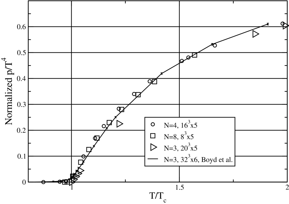
Figure 4.6: Results of lattice calculations by Bringoltz and Teper, (2005) of the pressure of pure SU($N$) Yang-Mills theory normalized to the pressure of a free gas for $N=3$ (triangles), $N=4$ (circles) and $N=8$ (squares). The solid line is the $N=3$ result of Boyd et al., (1996).

To obtain the pressure, the next-to-leading order gap equation was used. But as was argued by Root, (1974) one in principle only needs the leading order gap equation in order to obtain the value of the effective potential at the minimum. Writing the solution to the gap equations as

$$m^{2}=m^{2}_{\mathrm{LO}}+m^{2}_{\mathrm{NLO}}/N\;.$$ (4.64)

and Taylor expanding the effective potential, one obtains (up to $\mathcal{O}(1/N)$ corrections)

$$\mathcal{V}(m^{2})=N\mathcal{V}_{\mathrm{LO}}(m^{2}_{\mathrm{LO}})+\mathcal{V}_{\mathrm{NLO}}(m_{\mathrm{LO}}^{2})+m^{2}_{\mathrm{NLO}}\left.\frac{\partial\mathcal{V}_{\mathrm{LO}}(m^{2})}{\partial m^{2}}\right|_{m^{2}=m^{2}_{\mathrm{LO}}}$$ (4.65)

The last term of Eq. (4.65) vanishes by using the leading-order gap equation. The pressure $\mathcal{P}$ can now be written as

$$\mathcal{P}\equiv N\mathcal{P}_{\mathrm{LO}}+\mathcal{P}_{\mathrm{NLO}}$$ (4.66)

From the discussion above it follows that

$$\mathcal{P}_{\mathrm{LO}}=\mathcal{V}^{T}_{\mathrm{LO}}(m^{2}_{T})-\mathcal{V}^{T=0}_{\mathrm{LO}}(m^{2}_{0})\;,\;\;\;\;\;\;\;\mathcal{P}_{\mathrm{NLO}}=\mathcal{V}^{T}_{\mathrm{NLO}}(m^{2}_{T})-\mathcal{V}^{T=0}_{\mathrm{NLO}}(m^{2}_{0})\;,$$ (4.67)

where $m^{2}_{T}$ is the solution of the leading-order gap equation, at temperature $T$. By using the leading order gap equation it can be shown that at the minimum, part of $D_{2}$ becomes

$$\frac{1}{4\pi}\left[\Lambda^{2}\log\log\left(\frac{\Lambda^{2}}{\bar{m}^{2}}\right)-\bar{m}^{2}\,\mathrm{li}\left(\frac{\Lambda^{2}}{\bar{m}^{2}}\right)\right]=\\ \frac{\Lambda^{2}}{4\pi}\left[\log\left(\frac{4\pi}{g_{b}^{2}}\right)-\exp\left(-\frac{4\pi}{g_{b}^{2}}\right)\mathrm{li}\,\exp\left(\frac{4\pi}{g_{b}^{2}}\right)\right]\;.$$ (4.68)

Since $D_{2}$ contains the logarithmic integral it is dependent on the prescription and has an ambiguity. From Eq. (4.68) it follows that the problematic $T$-dependent divergences become $T$-independent at the minimum of the effective potential, and vanish in the calculation of the pressure due to the subtraction of the zero temperature contribution. As a result the pressure is unambiguous, i.e. independent of the choice of prescription.

4.6 High-temperature approximations

Bochkarev and Kapusta, (1996) consider the nonlinear sigma model in 3+1 dimensions, at next-to-leading order in the $1/N$ expansion. Since their result for the pressure cannot be obtained analytically, they resort to a “high-energy approximation”. In this section the same approximation for the $1+1$-dimensional case will be made to compare it with the exact numerical results obtained in Sec. 4.5.

The essence of the high-energy approximation of Bochkarev and Kapusta, (1996) is that one neglects the zero temperature part of $\Pi(P,m)$ and approximates it by its temperature-dependent part $\Pi_{T}(P,m)$. According to Bochkarev and Kapusta, (1996) one can then approximate $\Pi_{T}(P,m)$ by its high-energy behavior. In the present case of the nonlinear sigma model in $1+1$ dimensions, these approximations amount to

$$\Pi(P,m)\approx\Pi_{T}(P,m)\approx\frac{1}{4\pi}\frac{P^{2}}{(p_{0}^{2}+\omega_{+}^{2})(p_{0}^{2}+\omega_{-}^{2})}J_{1}\;,$$ (4.69)

where $\omega_{\pm}=\sqrt{p^{2}+m^{2}}\pm m$. This expression is identical to the high-momentum approximation to $\Pi_{T}(P,m)$, Eq. (4.48). In the high-energy approximation the effective potential is given by

$$\mathcal{V}_{\mathrm{HEA}}=\frac{Nm^{2}}{2g_{b}^{2}}-\frac{N}{2}\hbox{$\sum$}\!\!\!\!\!\!\int_{P}\log\left(P^{2}+m^{2}\right)-\frac{1}{2}\hbox{$\sum$}\!\!\!\!\!\!\int_{P}\log P^{2}\\ +\frac{1}{2}\hbox{$\sum$}\!\!\!\!\!\!\int_{P}\log\left(p_{0}^{2}+\omega_{+}^{2}\right)+\frac{1}{2}\hbox{$\sum$}\!\!\!\!\!\!\int_{P}\log\left(p_{0}^{2}+\omega_{-}^{2}\right)+\mathcal{O}(1/N)\;.$$ (4.70)

The resulting expression for the gap equation is

$$\frac{N}{g_{b}^{2}}=N\hbox{$\sum$}\!\!\!\!\!\!\int_{P}\frac{1}{P^{2}+m^{2}}-\hbox{$\sum$}\!\!\!\!\!\!\int_{P}\frac{\omega_{+}^{2}}{mE_{p}}\frac{1}{p_{0}^{2}+\omega_{+}^{2}}+\hbox{$\sum$}\!\!\!\!\!\!\int_{P}\frac{\omega_{-}^{2}}{mE_{p}}\frac{1}{p_{0}^{2}+\omega_{-}^{2}}\;.$$ (4.71)

Again, the gap equation requires coupling constant renormalization. In this approximation, it is found that the renormalization constant is

$$Z_{g^{2}}^{-1}=1+\frac{g^{2}}{4\pi}\left(1-\frac{2}{N}\right)\log\left(\frac{\Lambda^{2}}{\mu^{2}}\right)\;,$$ (4.72)

which differs slightly from the exact renormalization constant to next-to-leading order in $1/N$, Eq. (4.33). It is in fact equal to the perturbative one as for instance is discussed in Peskin and Schroeder, (1995). Making the substitution $g_{b}^{2}\rightarrow Z_{g^{2}}g^{2}$, one obtains

$$1=\frac{g^{2}}{4\pi N}\left[NJ_{1}-K_{1}^{+}-K_{1}^{-}+2(N-2)\log\frac{\mu}{m}\right]\;.$$ (4.73)

where the functions $K_{1}^{\pm}$ are defined as

$$K_{1}^{\pm}=\pm 4\int_{0}^{\infty}\frac{\mathrm{d}p\;\omega_{\pm}}{mE_{p}}n(\omega_{\pm})\;.$$ (4.74)

By substituting the gap equation (4.71) into the expression for the effective potential in the high-energy approximation, Eq. (4.70), the pressure becomes

$$\mathcal{P}_{\mathrm{HEA}}=\frac{N}{8\pi}\left[J_{0}T^{2}+(J_{1}-1)m^{2}\right]+\frac{\pi}{6}T^{2}\\ -\frac{1}{8\pi}\left[(K_{0}^{+}+K_{0}^{-})T^{2}+(K_{1}^{+}+K_{1}^{-}-2)m^{2}\right]\;,$$ (4.75)

where the functions $K_{0}^{\pm}$ are given by

$$K_{0}^{\pm}=\frac{8}{T^{2}}\int_{0}^{\infty}\frac{\mathrm{d}p\;p^{2}}{E_{p}}n(\omega_{\pm})\;.$$ (4.76)

Figure 4.7: Exact pressure as a function of temperature at next-to-leading order for $N=8$ compared with the high-energy and high-temperature approximations.

From Fig. 4.7, one can see that the high-energy approximation underestimates the pressure compared to the exact result. The advantage of an approximation like the high-energy approximation is that the analytic calculations are simpler and that it is easier to implement numerically. However, it is not a satisfactory approximation because one cannot really justify that the temperature-independent part of $\Pi(P,m)$ can be left out. It may even be considered surprising that this approximation works. In Chapter 6 it will be shown that the high-energy approximation in the nonlinear sigma model in $3+1$ dimensions actually leads to wrong results.

It is possible to derive a different approximation, which is better than the high-energy approximation. The inverse $\tilde{\alpha}$-propagator $\Pi$ at finite temperature can be obtained by first integrating over the momentum which gives

$$\Pi^{T}(P,m)=\frac{1}{2\beta}\sum_{q_{0}=2n\pi T}\frac{1}{\sqrt{m^{2}+q_{0}^{2}}}\frac{P^{2}+2q_{0}p_{0}}{P^{4}+4q_{0}(q_{0}+p_{0})P^{2}+4m^{2}p^{2}}\;.$$ (4.77)

Since it follows from the leading order gap equation that for high temperatures and for all values of the coupling constant, $m\ll T$ see Fig. 4.3, $\Pi(P,m)$ can at high temperatures (HT) be approximated by keeping only the $q_{0}=0$ mode in the sum Eq. (4.77) as follows

$$\Pi(P,m)\approx\Pi_{\mathrm{HT}}(P,m)=\frac{1}{2}\frac{1}{\beta m}\frac{P^{2}}{P^{4}+4m^{2}p^{2}}\;.$$ (4.78)

By using that $P^{4}+4m^{2}p^{2}$ can be written as $[p_{0}^{2}+(p+im)^{2}+m^{2}][p_{0}^{2}+(p-im)^{2}+m^{2}]$ and shifting $p\rightarrow p\pm im$ after taking the logarithm, it is found that

$$\hbox{$\Delta$}\!\!\!\!\!\!\int_{P}\log(P^{4}+4m^{2}p^{2})=2\hbox{$\Delta$}\!\!\!\!\!\!\int_{P}\log(P^{2}+m^{2})\;.$$ (4.79)

Hence the function $F_{1}$ can be approximated by

$$F_{1}\approx\hbox{$\Delta$}\!\!\!\!\!\!\int_{P}\log\Pi_{\mathrm{HT}}(P,m)=\frac{1}{2\pi}T^{2}J_{0}(\beta m)-\frac{\pi}{3}T^{2}\approx\frac{\pi}{3}T^{2}\;,$$ (4.80)

The function $F_{2}\approx 0$ in the high-temperature approximation because $\int_{P}\log\Pi_{HT}$ does not contain a finite term that depends on temperature. The part proportional to $\log\beta m$ gives rise to a divergence which by definition is not part of $F_{2}$. These high temperature limits agree with the numerical calculations displayed in Figs. 4.1 and 4.2.

The numerical calculation of $F_{1}+F_{2}$ shows that for $m/T\raisebox{-4.0pt}{$\,\stackrel{{\scriptstyle\textstyle<}}{{\sim}}\,$}0.1$ this approximation has an error smaller than $10$ percent. To obtain the pressure in the high-temperature approximation, Eq. (4.63) was applied using the approximations to $F_{1}$ and $F_{2}$. The result for the pressure in the high-temperature approximation is shown for comparison in Fig. 4.7 (again for $g^{2}(\mu=500)=10$). It can be seen that the high-temperature approximation is much better than the high-energy approximation.

One can approximate the pressure even further by expanding the functions $J_{0}$ and $J_{1}$ in the limit $\beta m\rightarrow 0$:

$$J_{0} = \frac{4\pi^{2}}{3}-4\pi\beta m-2\left(\log\frac{\beta m}{4\pi}+\gamma_{E}-\frac{1}{2}\right)(\beta m)^{2}+\mathcal{O}\left((\beta m)^{4}\right)\;,$$ (4.81)

$$J_{1} = \frac{2\pi}{\beta m}+2\left(\log\frac{\beta m}{4\pi}+\gamma_{E}\right)+\mathcal{O}\left((\beta m)^{2}\right)\;.$$ (4.82)

Inserting the approximations given in Eqs. (4.80), (4.81) and (4.82) into the gap equation (4.62), one obtains

$$\beta m\approx\pi\left[\left(\frac{2\pi}{g^{2}(\mu)}-\frac{\log 4}{N}\right)\left(1+\frac{2}{N}\right)-\gamma_{E}-\log\frac{\mu\beta}{4\pi}\right]^{-1}\;,$$ (4.83)

which indicates that $\beta m\sim 1/\log T$ for large $T$. In the limit $m/T\rightarrow 0$, the high-temperature approximation of the pressure is

$$\frac{\mathcal{P}}{NT^{2}}\approx\frac{\pi}{6}\left(1-\frac{1}{N}\right)-\left(1-\frac{2}{N}\right)\frac{m}{4T}\;,$$ (4.84)

where the first term is the pressure of a gas of free massless particles with $N-1$ degrees of freedom.

4.7 Thermal infrared renormalons

An observable $O$ in a quantum field theory like QCD is often only known in terms of an expansion in the coupling constant $\alpha$. Because negative $\alpha$ gives rise to unphysical behavior as was argued by Dyson, (1952) for QED, it is expected that this series expansion has zero radius of convergence. Hence one should view it at best as an asymptotic series. One might wonder whether it is possible by resumming the series expansion to learn about the non-perturbative physics. In specific cases this is possible, but more often one finds so-called renormalons, which give rise to ambiguities in the relation between $O$ and its resummed version. These ambiguities may give an insight in the size of the non-perturbative corrections.

Since one can apply the $1/N$ expansion to the nonlinear sigma model, observables can be calculated exactly in terms of the coupling constant. These exact expressions can be used to study the renormalons in the nonlinear sigma model as was done at zero temperature by David, (1982, 1984, 1986) and Beneke et al., (1998). In this section this analysis is extended to finite temperature.

This section consists of two parts. In the first part a short introduction into renormalons will be given. In the second part the nonlinear sigma model will be used to investigate the temperature dependence of the renormalons and how they affect the possible definitions of the renormalized effective potential, pressure and gap equation. For a more extensive review on renormalons see Altarelli, (1995) and Beneke, (1999).

Renormalons

An observable $O$ can in general be expressed in terms of a perturbation series in $\alpha=g^{2}$ in the following way

$$O(\alpha)\sim\sum_{n=0}^{\infty}a_{n}\alpha^{n}\;.$$ (4.85)

It often happens that this series is an asymptotic series which is not convergent. Such an asymptotic series can sometimes be resummed by the Borel transform method, although in general this resummation is not unique. The Borel transform of $O(\alpha)$ is defined as

$$B(t)=\sum_{n=0}^{\infty}\frac{a_{n}}{n!}t^{n}\;.$$ (4.86)

The observable $O$ can now be expressed in terms of an integral over its Borel transform

$$O(\alpha)=\frac{1}{\alpha}\int_{0}^{\infty}\mathrm{d}t\,e^{-t/\alpha}B(t)\;,$$ (4.87)

which has the series expansion of Eq. (4.85). For example if one takes $a_{n}=(-1)^{n}n!$, the series expansion for $O$ is clearly divergent. The Borel transform however is convergent for $|t|<1$ and equal to $B(t)=1/(1+t)$. To resum $O(\alpha)$ it is assumed that $B(t)=1/(1+t)$ for any value of $t$. The resummed expression for $O$ now yields

$$O(\alpha)=\frac{1}{\alpha}\int_{0}^{\infty}\mathrm{d}t\,e^{-t/\alpha}\frac{1}{1+t}\;.$$ (4.88)

The integral in Eq. (4.88) is convergent and, moreover, well-defined since there are no singularities along the integration contour. So in this example the asymptotic series has been resummed unambiguously. However, sometimes this method gives rise to ambiguities. Take for example $a_{n}=n!$ in which case $B(t)=1/(1-t)$ and

$$O(\alpha)=\frac{1}{\alpha}\int_{0}^{\infty}\mathrm{d}t\,e^{-t/\alpha}\frac{1}{1-t}\;.$$ (4.89)

In this case the integral is not well defined since there is a singularity at $t=1$ on the integration contour. This singularity is called the renormalon pole. One can still give a meaning to this resummed series by introducing a prescription how to integrate around the pole

$$O(\alpha)_{\pm}=\frac{1}{\alpha}\int_{0}^{\infty}\mathrm{d}t\,e^{-t/\alpha}\frac{1}{1-t\pm i\epsilon}\;.$$ (4.90)

This resummation gives rise to ambiguities, since one does not know whether to take the $+$, $-$ or a combination like the principal value prescription. But as long as the differences between the prescriptions are not that big, it does not really matter. The difference is equal to the residue at $t=1$, which is called the renormalon residue. In this case it is equal to

$$O(\alpha)_{+}-O(\alpha)_{-}=\frac{2\pi i}{\alpha}\exp\left(-1/\alpha\right)\;.$$ (4.91)

So in this example the series can be resummed up to ambiguities of order $\exp(-1/\alpha)/\alpha$. These ambiguities are tiny when $\alpha$ is small. However for larger values of $\alpha$ they can become important. These ambiguities indicate that the non-perturbative corrections to Eq. (4.85) could be in this case of order $\exp(-1/\alpha)/\alpha$.

Renormalons in the nonlinear sigma model

Renormalons appear in the vacuum expectation value of the $\alpha$ field. A calculation shows that at zero temperature one can write (David, , 1986)

$$\left<\alpha\right>=m_{\mathrm{LO}}^{2}+\frac{4\pi m_{\mathrm{LO}}^{2}}{N}\int\frac{\mathrm{d}^{2}P}{(2\pi)^{2}}\frac{1}{\Pi}\frac{\partial\Pi}{\partial m_{\mathrm{LO}}^{2}}+\mathcal{O}\left(\frac{1}{N^{2}}\right)\;,$$ (4.92)

where $m_{\mathrm{LO}}^{2}\equiv\Lambda^{2}\exp(-4\pi/g_{b}^{2})$. This equation is in agreement with the gap equation (4.28) if $m^{2}$ is split as follows $m^{2}=m_{\mathrm{LO}}^{2}+m_{\mathrm{NLO}}^{2}/N$. The part of the integral in Eq. (4.92) that has the infrared renormalon pole in the Borel plane is in fact the contribution from the integrand in the limit $P^{2}/m^{2}\to\infty$ (its “perturbative tail”)

$$\int^{\Lambda}\frac{\mathrm{d}^{2}P}{(2\pi)^{2}}\frac{1}{\Pi_{\infty}}\frac{\partial\Pi_{\infty}}{\partial m^{2}}=-\frac{1}{4\pi}{\mathrm{li}}\left(\frac{\Lambda^{2}}{m^{2}}\right)=-\frac{1}{4\pi}\frac{\Lambda^{2}}{m^{2}}e^{-x}{\mathrm{Ei}}(x)\;,$$ (4.93)

where $x=\log(\Lambda^{2}/m^{2})$ and $\mathrm{Ei}(x)$ the exponential integral which is defined below. In the limit $x\to\infty$, the logarithmic integral has the asymptotic expansion

$$e^{-x}{\mathrm{Ei}}(x)=\sum_{n=0}^{\infty}\frac{n!}{x^{n+1}}\mp i\pi e^{-x}=\int_{0}^{\infty}\mathrm{d}b\,\frac{e^{-bx}}{1-b}\mp i\pi e^{-x}\;,$$ (4.94)

where $\arg(b)=\pm\varepsilon$. From Eq. (4.94), it is clear that there is a renormalon pole at $b=1$. This shows that when $\Lambda\to\infty$ the value of $\left<\alpha\right>$ is inherently ambiguous at next-to-leading order, due to the freedom in the choice of prescription. David, (1984) has shown that this ambiguity also arises in dimensional regularization.

The same problem appears in the calculation of the effective potential even at its minimum, but not in the gap equation. The latter can be seen from the last term of Eq. (4.20) which contributes to the gap equation as follows

$$\frac{1}{2}\frac{\partial}{\partial m^{2}}\int\frac{\mathrm{d}^{2}P}{(2\pi)^{2}}\log\Pi=\frac{1}{2}\int\frac{\mathrm{d}^{2}P}{(2\pi)^{2}}\frac{1}{\Pi}\frac{\partial\Pi}{\partial m^{2}}\;.$$ (4.95)

The ambiguity that would arise from this term when removing its perturbative tail (cf. Eq. (4.93)) cancels in the gap equation (4.28) against the one arising in $m^{2}$ (cf. Eq. (4.92)).

The perturbative tail of the effective potential, i.e. the first two terms of $D_{2}$ defined in Eq. (4.54), corresponds to poles in the Borel plane at $b=0$ and $b=1$, respectively. Since $\bar{m}^{2}$ is only temperature independent at the minimum (at LO only, but that is sufficient because one is working at NLO), the subtraction of the perturbative tail will become temperature dependent, except at the minimum. Since subtracting temperature-dependent divergences renders the remaining temperature-dependent terms meaningless, it is impossible to define a finite effective potential at finite temperature. In order to avoid any renormalon ambiguity, it also not possible to obtain a finite effective potential or even an unambiguous minimum at zero temperature. However, as was shown in Sec. 4.5 the quantity $\mathcal{P}^{T}-\mathcal{P}^{T=0}$ is free from renormalon ambiguities and is finite after temperature-independent coupling constant renormalization.

Finally, using Eq. (4.92) one can investigate the finite temperature dependence of renormalon contributions to $\langle\alpha\rangle$ and the effective potential. One can show that Eq. (4.92) at finite temperature has exactly the same renormalon contribution, i.e. neither the pole nor the residue become temperature dependent. Secondly, the perturbative tail of the effective potential which is given by the first two terms of $D_{2}$, corresponds to poles in the Borel plane at $b=0$ and $b=1$. The positions of the renormalon poles are not affected by temperature. Only the residues become temperature dependent, except at the minimum of the potential, as we concluded earlier. The fact that renormalon pole positions are not affected by temperature, but residues are, is also the case for the thermal ultraviolet renormalons in $\phi^{4}$ in $3+1$ dimensions studied by Loewe and Valenzuela, (2000).

4.8 Summary and Conclusions

To summarize, the pressure in the nonlinear sigma model was calculated at finite temperature to next-to-leading order in the $1/N$ expansion. The main result is that one can obtain an unambiguous, finite pressure, by subtracting the zero-temperature value of the pressure and renormalization of the coupling constant in a temperature-independent way. This procedure cannot be carried out away from the minimum of the effective potential and it was argued that defining a finite, effective potential by the subtraction of the so-called perturbative tail, leads to ambiguities associated with infrared renormalons. In general, these become temperature dependent, and this casts doubt on the usefulness of defining a finite effective potential outside the minimum. Since it turns out that, as it should, physical quantities are independent of the choice of prescription, one can apply any prescription for the logarithmic integral without worrying about the possible ambiguities. This is what will be done in the remaining chapters of this thesis.

The expression for the pressure was calculated numerically at finite temperature. This calculation shows that the $1/N$ expansion is a meaningful expansion for all temperatures. The high-energy approximation that was originally applied to the nonlinear sigma model in 3+1 dimensions by Bochkarev and Kapusta, (1996) was also studied. In 1+1 dimensions, where one can compare with exact numerical results, it was found that it underestimates the pressure for all temperatures. An improved approximation was suggested, the so-called high-temperature approximation. This approximation has the advantage that it is quite easy to produce numerical results and agrees better with the exact results. At asymptotically high temperatures the pressure approaches that of a gas of $N-1$ free massless particles. It was found that the pressure divided by the pressure at infinite temperatures has a very weak dependence on $N$. Similarly behavior is found in lattice calculations as a function of $N_{f}$ and $N_{c}$.

Chapter 5 Thermodynamics of the $\boldsymbol{\mathbb{C}P^{N-1}}$ model

Using the $1/N$ expansion, the influence of quantum instantons to the thermodynamics of the $\mathbb{C}P^{N-1}$ model in 1+1 dimensions is studied. The auxiliary field effective potential is calculated to next-to-leading order in $1/N$ and turns out to have temperature-dependent ultraviolet divergences. These divergences can only be renormalized at its minimum just like in the nonlinear sigma model discussed in Chapter 4. By using that the $\mathbb{C}P^{1}$ model is equivalent to the $\mathrm{O}(3)$ nonlinear sigma model it is argued that the pressure for intermediate temperatures is dominated by the effect of quantum instantons. This chapter is based on: The effect of quantum instantons on the thermodynamics of the $\mathbb{C}P^{N-1}$ model, J.O. Andersen, D. Boer and H.J. Warringa, hep-th/0602082.

5.1 Introduction

It was discovered by Belavin et al., (1975) that the classical equations of motion of Euclidean QCD have finite action solutions with nontrivial topology. These solutions are called instantons. They are stationary points of the classical action. In perturbation theory one most often only takes into account the trivial vacuum and small fluctuations around it. However, in the non-perturbative regime the instanton solutions and the fluctuations around it can really contribute to physical quantities as was first observed by ’t Hooft, (1976). He showed that instantons are giving rise to an additional source of $\mathrm{U}(1)_{A}$ symmetry breaking in QCD, which is necessary to explain the relatively large mass of the $\eta$ meson.

In this chapter it is investigated whether instantons can have an influence on the thermodynamical quantities. To answer this question, the $\mathbb{C}P^{N-1}$ model in $1{+}1$ dimensions will be studied since it admits instanton solutions for all $N$. The $\mathbb{C}P^{N-1}$ model was introduced by Eichenherr, (1978). It is possible to investigate its non-perturbative regime using the $1/N$ expansion (D’Adda et al., , 1978). An attractive feature of the $\mathbb{C}P^{N-1}$ model in $1{+}1$ dimensions are its similarities with QCD in $3{+}1$ dimensions. Like QCD it is an asymptotically free theory. Moreover, classically the $\mathbb{C}P^{N-1}$ model is scale-invariant. Due to renormalization of the quantum corrections a mass scale is introduced in the model. Furthermore, a mass gap for the scalar fields is generated dynamically by the interactions. The local $\mathrm{U}(1)$ symmetry of the $\mathbb{C}P^{N-1}$ model generates a long range interaction between the scalar fields. Since the Coulomb potential in ${1+1}$ dimensions is proportional to the distance between the charges, this model has confinement (D’Adda et al., , 1978). Finally as alluded to above, the classical equations of motion of the $\mathbb{C}P^{N-1}$ model admit instanton solutions (Golo and Perelomov, , 1978). Lazarides, (1979) investigated the $\mathbb{C}P^{N-1}$ model at finite temperature for the first time and showed that at non-zero temperature the model is no longer confining. For a review on the $\mathbb{C}P^{N-1}$ model at finite temperature, see Actor, (1985). Instantons in QCD at finite temperature are discussed by Gross et al., (1981) and in the large $N_{c}$ limit by Schäfer, (2004).

As is explained in Chapter 3, thermodynamical quantities like the pressure can be obtained by minimizing the finite temperature effective potential. In this chapter the finite temperature effective potential will be calculated to next-to-leading order in $1/N$. Its zero-temperature counterpart was calculated by Campostrini and Rossi, (1992). It turns out that the effective potential contains temperature-dependent ultraviolet divergences. These divergences become temperature-independent at the minimum. Thermodynamic quantities like the pressure are defined at the minimum of the effective potential and hence can be calculated without such renormalization problems. The same phenomenon is also found in the $\mathrm{O}(N)$ nonlinear sigma model in $1{+}1$ dimensions (Chapter 4) and the $\mathrm{O}(N)$ linear sigma model in $3{+}1$ dimensions (Chapter 6). A general explanation of how these temperature divergences arise is given in Sec. 3.4.

Instantons are characterized by a quantized winding number $Q$, which is a topological invariant. The instantons give a contribution proportional to $\exp(-\pi NQ/g_{b}^{2})$ to the partition function, where the non-analyticity in $g_{b}^{2}$ shows that the contribution is non-perturbative. This contribution also indicates that instantons effects disappear in the limit $N\rightarrow\infty$ as was argued by Witten, (1979). As a result one has to perform calculations to next-to-leading order in $1/N$ to investigate the effects of instantons in the $1/N$ expansion. It was argued by Witten, (1979) using the $1/N$ expansion at zero temperature that quantum corrections let the instanton configurations to disappear. However, Jevicki, (1979) showed that classical instantons still are present in the quantum effective action, not longer as stationary solutions but as poles. However, at finite temperature, Affleck, (1980a, b, c) found that the large-$N$ quantum effective action does contain stationary solutions with quantized topological charge, called quantum instantons. Hence, at finite temperature configurations with non-trivial topology can contribute to physical quantities. In this chapter the same conclusion will be drawn. The pressure is calculated for topological configurations with zero winding number. The contribution from other configurations will be ignored since they are difficult to calculate. It is found that for intermediate temperatures, where the leading order contribution to the pressure divided by $T^{2}$ displays a sharp increase, the next-to-leading $1/N$ contributions gives rise to a negative pressure. This is unphysical because it results in a negative entropy. Therefore, the negative pressure indicates that an important contribution, most probably from the configurations with non-zero winding number, is left out. This conclusion is further strengthened by using a correspondence discovered by Eichenherr, (1978) between the $\mathbb{C}P^{1}$ model and the $\mathrm{O}(3)$ nonlinear sigma model. In the $1/N$ approximation of the $\mathrm{O}(3)$ nonlinear sigma model one implicitly includes all instanton configurations. Hence the difference between the pressure of the $Q=0$ sector of the $\mathbb{C}P^{1}$ model and the pressure of the $\mathrm{O}(3)$ nonlinear sigma model gives the contribution of the topological configurations with $Q\neq 0$ to the pressure of the $\mathbb{C}P^{1}$ model. In this way a strong hint is found that the topological configurations with $Q\neq 0$ give a large contribution to the pressure for intermediate temperatures.

This introduction will be ended by mentioning some related studies of the $\mathbb{C}P^{N-1}$ model. Schwab, (1982), Münster, (1982) and Münster, (1983) have investigated the $\mathbb{C}P^{N-1}$ model on the sphere $S^{2}$. Münster, (1983) remarked that it is naive to expand only around the saddle point $A_{\mu}=0$ because it leads to an improper treatment of zero modes. Furthermore, the $\mathbb{C}P^{N-1}$ model has been studied on the lattice as well, see for example Campostrini et al., (1992a, b) and Vicari, (1993). A way to investigate the relevance of the topological solutions is by adding a term $\vartheta Q$ to the action. Olejnik and Schierholz, (1994) and Schierholz, (1995) calculated for $N=4$ the free energy as a function of $\vartheta$. They found that depending on the size of the coupling constant there is a phase transition from the confined to the deconfined phase for $\vartheta\leq\pi$. Azcoiti et al., (2004) found that for $N=10$ the CP symmetry is spontaneously broken for $\vartheta=\pi$. The $\mathbb{C}P^{N-1}$ model also has applications in condensed matter physics. Pruisken et al., (2003) and Pruisken and Burmistrov, (2005) have applied this model to investigate the quantum Hall effect. Ichinose and Yamamoto, (1990) studied antiferromagnetism using the $\mathbb{C}P^{N-1}$ model at finite temperature.

This chapter is organized as follows. In Sec. 5.2 the $\mathbb{C}P^{N-1}$ model is introduced. The calculation of the effective action and effective potential are performed in Secs. 5.3 and 5.4. In Sec. 5.5 the results of the calculation of the pressure are discussed. Finally a summary and conclusions are given in Sec. 5.6.

5.2 The $\mathbb{C}P^{N-1}$ model

The $\mathbb{C}P^{N-1}$ model is described by the following Lagrangian density

$$\mathcal{L}=\frac{1}{2}\partial_{\mu}\phi_{i}^{*}\partial^{\mu}\phi_{i}+\mathcal{L}_{\mathrm{int}}\;,\;\;\;\;\;\;\;\phi_{i}^{*}\phi_{i}=N/{g_{b}^{2}}\;,\;\;\;\;\;\;\;i=1\ldots N\;,$$ (5.1)

where $\phi(x)$ is a complex scalar field and $g_{b}$ is the bare coupling constant. Under an $\mathrm{U}(1)$ transformation which is parametrized by $\sigma(x)$, $\phi(x)\rightarrow\exp[i\sigma(x)]\phi(x)$. By requiring that the Lagrangian density is invariant under local $\mathrm{U}(1)$ transformations, the interaction term $\mathcal{L}_{\mathrm{int}}$ can be determined from the transformation rule of the Lagrangian density which reads

$$\delta\mathcal{L}=i(\partial_{\mu}\sigma)\left(\partial^{\mu}\phi_{i}^{*}\right)\phi_{i}+\delta\mathcal{L}_{\mathrm{int}}=0\;.$$ (5.2)

Hence the interaction term should contain derivatives. If the interaction Lagrangian density is chosen as follows

$$\mathcal{L}_{\mathrm{int}}=\frac{g_{b}^{2}}{2N}\left(\phi_{i}^{*}\partial_{\mu}\phi_{i}\right)\left(\phi_{j}^{*}\partial^{\mu}\phi_{j}\right)\;,$$ (5.3)

then Eq. (5.2) is satisfied. As a result the model becomes invariant under global $\mathrm{SU}(N)$ transformations as well.

The Lagrangian density can also be written in terms of gauge fields $A_{\mu}$ which transform under a $\mathrm{U}(1)$ gauge transformation as

$$A_{\mu}(x)\rightarrow A^{\prime}_{\mu}(x)=A_{\mu}(x)-\partial_{\mu}\sigma(x)\;.$$ (5.4)

The Lagrangian density expressed in gauge fields is given by

$$\mathcal{L}=\frac{1}{2}\left|\mathcal{D}_{\mu}\phi_{i}\right|^{2}\;,\;\;\;\;\;\;\;\phi_{i}^{*}\phi_{i}=N/{g_{b}^{2}}\;.$$ (5.5)

where the covariant derivative $\mathcal{D}_{\mu}=\partial_{\mu}+iA_{\mu}$. By solving the equations of motions of the $A_{\mu}$ fields one finds

$$A_{\mu}=i\frac{g_{b}^{2}}{N}\phi_{i}^{*}\partial_{\mu}\phi_{i}^{\phantom{*}}\;.$$ (5.6)

If this expression is inserted into Eq. (5.5) the original Lagrangian density Eq. (5.1) and Eq. (5.3) is recovered.

Coset models

The $\mathbb{C}P^{N-1}$ and the $\mathrm{O}(N)$ nonlinear sigma model are examples of coset models. A coset model is a theory of fields $\phi(x)$ which take values in the coset space $G/H$. Here $G$ denotes a compact Lie group and $H$ a closed subgroup of $G$. The coset space $G/H$ is a manifold though only a Lie group if $H$ is an invariant subgroup of $G$. The coset space has dimension $\mathrm{dim}\,G/H=\mathrm{dim}\,G-\mathrm{dim}\,H$. In 2-dimensional Euclidean space, $\phi$ is a map from $\mathbb{R}^{2}\rightarrow G/H$, whereas at finite temperature this map becomes $S\times\mathbb{R}\rightarrow G/H$. In a coset model the fields transform as $\phi(x)\rightarrow g\phi(x)$ where $g\in G$. The Lagrangian density of a coset model is given by

$$\mathcal{L}=\frac{1}{2}\eta^{\mu\nu}g^{ij}(\phi)\partial_{\mu}\phi^{*}_{i}\partial_{\nu}\phi^{\phantom{*}}_{j}\;,$$ (5.7)

where $\eta_{\mu\nu}$ is the space-time metric ($\delta_{\mu\nu}$ in Euclidean space) and $g_{ij}(\phi)$ is a metric on the coset space $G/H$. The metric $g_{ij}$ is to be chosen in such a way that the Lagrangian density is invariant under transformations $G$.

Coset models have an interesting connection to the topology of space-time. If one identifies all points at space-time infinity, the fields $\phi(x)$ become a map from $S^{2}\rightarrow G/H$. These maps can be topologically nontrivial, which implies that there are maps $\phi(x)$ which cannot be deformed continuously into each other. Such maps can be classified according to the second homotopy group of $G/H$, $\pi_{2}(G/H)$. In the case that the second homotopy group is nontrivial, the action of the coset model has more than one stationary solution, which in Euclidean space-time are called instantons. At finite temperature all points at $x_{1}=\pm\infty$ can be identified, as a result space-time becomes $S^{2}$ as well. Hence finite temperature instantons (also called calorons) do exist, but unlike instantons at zero temperature they satisfy the boundary conditions for scalar fields in imaginary time (Lazarides, , 1979; Affleck, , 1980a; Gross et al., , 1981; Bruckmann et al., , 2005).

The $\mathrm{O}(N)$ nonlinear sigma model is an $\mathrm{O}(N)/\mathrm{O}(N-1)\cong S^{N-1}$ coset model with real scalar fields. Since in a coset model, the fields take their value in the coset space, it follows that $\phi_{i}\phi_{i}=N/g_{b}^{2}$, where $i=1\ldots N$ and $N/g_{b}^{2}$ is the radius of $S^{N-1}$. If the metric is chosen to be $g_{ij}=\delta_{ij}$ the Lagrangian density becomes invariant under G. Furthermore the Lagrangian density discussed in Chapter 4, Eq. (4.1), is recovered from Eq. (5.7) in this way. Since $\pi_{2}(S^{N-1})\neq 0$ only for $N=3$, the $\mathrm{O}(N)$ nonlinear sigma model has instanton solutions for $N=3$ only.

The $\mathbb{C}P^{N-1}$ model is an $\mathrm{SU}(N)/\mathrm{U}(N-1)\cong\mathbb{C}P^{N-1}$ coset model. The space $\mathbb{C}P^{N-1}$ is the so-called complex projective space, it is the space of $N$-dimensional complex vectors $z$ satisfying the equivalence relation $z\sim z^{\prime}$ if $z=\lambda z^{\prime}$ where $\lambda\in\mathbb{C}$ and the relation $z^{\dagger}z=c$. Hence the $N$ scalar fields $\phi_{i}(x)$ of the $\mathbb{C}P^{N-1}$ model satisfy $\phi_{i}^{*}(x)\phi_{i}(x)=N/g_{b}^{2}$. The equivalence relation together with the constraint directly translates into the requirement of $\mathrm{U}(1)$ gauge invariance. The corresponding metric on the coset space can be read off from Eq. (5.3), $g_{ij}=\delta_{ij}+g_{b}^{2}\phi^{\phantom{*}}_{i}\phi^{*}_{j}/N$. It turns out that $\pi_{2}(\mathbb{C}P^{N-1})=\mathbb{Z}$, hence the $\mathbb{C}P^{N-1}$ model has instanton solutions for any $N$.

Instantons

Classical instantons are solutions to the classical equations of motion in Euclidean space-time which have finite action. They can be characterized by an integer topological charge $Q$ which is given by

$$Q=\frac{1}{2\pi i}\frac{g_{b}^{2}}{N}\int\mathrm{d}^{2}x\,\epsilon_{\mu\nu}\partial_{\mu}\left(\phi_{i}^{*}\partial_{\nu}\phi_{i}^{\phantom{*}}\right)\;.$$ (5.8)

Using Eq. (5.6) the expression for $Q$ can be written in terms of the gauge field as follows

$$Q=\frac{1}{2\pi}\int\mathrm{d}^{2}x\,\epsilon_{\mu\nu}\partial_{\mu}A_{\nu}\;.$$ (5.9)

To show that $Q$ is an integer, consider a configuration with finite action. In that case the fields $\phi$ should go to a constant times a phase factor (arising from gauge invariance) at infinity, $\lim_{x\rightarrow\infty}\phi(x)\equiv\phi_{\infty}\exp[i\sigma(x)]$. Since $Q$ is the integral over a total divergence, it can be written as a surface integral at infinity. As a result one finds

$$Q=\frac{1}{2\pi}\int_{0}^{2\pi}\mathrm{d}\vartheta\,\frac{\mathrm{d}\sigma({R=\infty},\vartheta)}{\mathrm{d}\vartheta}=\frac{1}{2\pi}\Delta\sigma\;,$$ (5.10)

where $\Delta\sigma$ denotes the change in $\sigma$ by going along a circle at infinity. Since the fields with finite action should be continuous functions, $\sigma$ is a multiple of $2\pi$. Hence $Q$ can only take integer values.

Like any vector, $C_{\mu}^{i}=\mathcal{D}_{\mu}\phi^{i}$ satisfies $|C_{\mu}^{i}\pm i\epsilon_{\mu\nu}C_{\nu}^{i}|^{2}\geq 0$. Working out this equation gives a lower bound on the Lagrangian density of the $\mathbb{C}P^{N-1}$ model

$$\mathcal{L}\geq\pm\tfrac{1}{2}i\epsilon_{\mu\nu}\partial_{\mu}\left(\phi^{*}_{i}\partial_{\nu}\phi_{i}^{\phantom{*}}\right)=\pm\frac{N}{2g_{b}^{2}}\epsilon_{\mu\nu}\partial_{\mu}A_{\nu}\;.$$ (5.11)

Integrating this equation over $x$ results in the classical action $S$ which satisfies the following lower bound

$$S\geq\frac{\pi N}{g_{b}^{2}}\left|Q\right|\;.$$ (5.12)

For instantons this lower bound turns into an equality. The explicit form of the instantons can be found by solving the self-duality equation

$$\mathcal{D}_{\mu}\phi_{i}=\pm i\epsilon_{\mu\nu}\mathcal{D}_{\nu}\phi_{i}\;.$$ (5.13)

The solutions of this equation, the instantons, are of the following form (Golo and Perelomov, , 1978)

$$\phi_{i}(x)=\left({N}/{g_{b}^{2}}\right)^{1/2}e^{i\sigma(x)}\frac{w_{i}(x_{0}\pm ix_{1})}{\left|w(x_{0}\pm ix_{1})\right|}\;,$$ (5.14)

where $w(x_{0}\pm ix_{1})$ is a smooth $N$-dimensional complex vector function. The one instanton (with $Q=1$) for example can be written as (Golo and Perelomov, , 1978; D’Adda et al., , 1978)

$$\phi_{i}(x)=\frac{\lambda u_{i}+\left[(x_{0}-a_{0})-i(x_{1}-a_{1})\right]v_{i}}{\left(\lambda^{2}+(x-a)^{2}\right)^{1/2}}\;,$$ (5.15)

where $a_{\mu}$ is the position of the instanton in space and $\lambda$ the size of the instanton. The constants $u$ and $v$ obey the following relations, $|u|^{2}=N/g_{b}^{2}$, $|v|^{2}=N/g_{b}^{2}$ and $u^{*}\cdot v=0$.

These results can be generalized to finite temperature. If all points at $x_{1}=\pm\infty$ are identified the space changes from $S\times\mathbb{R}$ into $S^{2}$. To obtain a finite action at non-zero temperature, the fields $\phi$ still have to go to a constant, $\lim_{x\rightarrow\infty}\phi(x)\equiv\phi_{\infty}\exp[i\sigma(x)]$. Due to the finite temperature boundary condition $\sigma(x_{0},x_{1})=\sigma(x_{0}+\beta,x_{1})+2\pi N$. The topological charge is still quantized at finite temperature (Affleck, , 1980a). The action has the same bound as at zero temperature. The explicit form of the instanton at finite temperature (also called calorons) follow from solving the self-duality equations using the boundary condition on $x_{0}$, see Affleck, (1980b).

A correspondence between $\boldsymbol{\mathbb{C}P^{1}}$ and $\boldsymbol{\mathrm{O}(3)}$

The $\mathbb{C}P^{1}$ model is equivalent to the $\mathrm{O}(3)$ nonlinear sigma model, which was shown by Eichenherr, (1978), see also Banerjee, (1994). This means that there is a one-to-one correspondence between those two models. Such an equivalence for example implies that one can obtain the pressure of the $\mathbb{C}P^{1}$ model by calculating the pressure of the $\mathrm{O}(3)$ nonlinear sigma model. The correspondence can be made explicit by writing the $\mathrm{O}(3)$ nonlinear sigma fields $\chi(x)$ as follows

$$\chi_{a}(x)=\left(g_{b}^{2}/N\right)^{1/2}\phi^{*}_{i}(x)(\sigma_{a})^{\phantom{**}}_{ij}\phi^{\phantom{*}}_{j}(x)\;,\;\;\;\;\;\;\;\;a=1\ldots 3\;,$$ (5.16)

where $\sigma_{a}$ are the three $2\times 2$ Pauli matrices satisfying $\{\sigma_{a},\sigma_{b}\}=2\delta_{ab}$. Using Eq. (5.16) the $\mathrm{O}(3)$ nonlinear sigma Lagrangian density, Eq. (4.1), with constraint turns into the $\mathbb{C}P^{1}$ Lagrangian density, Eq. (5.1), with the corresponding constraint.

5.3 Effective action

To obtain the effective action, the constraint from Eq. (5.1) can be implemented by introducing an auxiliary Lagrange multiplier field $\alpha$. This gives rise to the following Lagrangian density which is equivalent to the original Lagrangian density Eq. (5.1)

$$\mathcal{L}=\frac{1}{2}\left|\mathcal{D}_{\mu}\phi_{i}\right|^{2}-\frac{i}{2}\alpha\left(\phi_{i}^{*}\phi^{\phantom{*}}_{i}-N/g_{b}^{2}\right)$$ (5.17)

Since the Lagrangian density is now quadratic in the $\phi$ fields, the Gaussian integration over these fields can be performed. This results in the following effective action

$$S_{\mathrm{eff}}=N\mathrm{Tr}\,\log\left(-\mathcal{D}_{\mu}\mathcal{D}^{\mu}-i\alpha\right)+i\frac{N}{2g_{b}^{2}}\int\mathrm{d}^{2}x\,\alpha(x)\;.$$ (5.18)

The covariant derivative $\mathcal{D}_{\mu}$ transforms as $U^{\dagger}\mathcal{D}_{\mu}U$. Hence, as expected this effective action is invariant under local $\mathrm{U}(1)$ transformations. In order to obtain the effective potential, $S_{\mathrm{eff}}$ has to be expanded around the vacuum expectation values of the $\alpha$ field. The vacuum expectation value of the $\alpha$ field is purely imaginary as is proved in Eq. (4.12). Therefore $\alpha$ can be expressed in terms of the sum of its vacuum expectation value $im^{2}$ and a quantum fluctuating field $\tilde{\alpha}$ as follows, $\alpha=im^{2}+\tilde{\alpha}/\sqrt{N}$. For convenience the gauge fields are rescaled by a factor $\sqrt{N}$. This rescaling with factors of $\sqrt{N}$ does not have any effect on the final results since the $\mathrm{\tilde{\alpha}}$ and $A_{\mu}$ fields are integration variables of the path integral. It is just a convenient way to organize the $1/N$ expansion. Working out the square of the covariant derivative and inserting the vacuum expectation value gives the following effective action

$$S_{\mathrm{eff}}=N\mathrm{Tr}\,\log\left(-\partial^{2}+m^{2}-\frac{i}{\sqrt{N}}\left\{\partial_{\mu},A^{\mu}\right\}+\frac{1}{N}A_{\mu}A^{\mu}-i\frac{\tilde{\alpha}}{\sqrt{N}}\right)\\ -\frac{N}{2g_{b}^{2}}\int\mathrm{d}^{2}x\left[m^{2}-\frac{i}{\sqrt{N}}\tilde{\alpha}(x)\right]\;.$$ (5.19)

Now as shown by Affleck, (1980a) $S_{\mathrm{eff}}$ contains stationary solutions $A_{\mu}$ at finite temperature, which vanish at zero temperature according to Witten, (1979). These solutions have a quantized topological charge given by Eq. (5.9). Since these solutions are stationary points of an action in which quantum effects are incorporated, they are called ‘quantum instantons’. In the limit of high temperature, the exact form of these quantum instantons can be found (Affleck, , 1980a). Such instantons need to be considered in a full calculation of the pressure. As a first step to investigate the relevance of the quantum instantons to the pressure, only the fluctuations around the trivial configuration $A_{\mu}=0$ are taken into account in this chapter. The result for the pressure of the $\mathbb{C}P^{1}$ model with $Q=0$ will be compared to the pressure of the $\mathrm{O}(3)$ nonlinear sigma model in which the contribution of all quantum instantons is take into account. Because the $\mathbb{C}P^{1}$ model is equivalent to the $\mathrm{O}(3)$ nonlinear sigma model this comparison should therefore give the contribution to the pressure of the quantum instantons.

To obtain the pressure for the $Q=0$ configuration, $S_{\mathrm{eff}}$ has to be expanded around the vacuum expectation value $im^{2}$ and the trivial configuration $A_{\mu}=0$ (with $Q=0$). Expanding $S_{\mathrm{eff}}$ gives

$$S_{\mathrm{eff}}=N\mathrm{Tr}\,\log\left(-\partial^{2}+m^{2}\right)+N\mathrm{Tr}\,\sum_{k=1}^{\infty}\frac{(-1)^{k+1}}{k}\left(\frac{\frac{1}{N}A_{\mu}A^{\mu}+\frac{1}{\sqrt{N}}\tilde{\alpha}-\frac{i}{\sqrt{N}}\left\{\partial_{\mu},A^{\mu}\right\}}{-\partial^{2}+m^{2}}\right)^{k}\\ -\frac{N}{2g_{b}^{2}}\int\mathrm{d}^{2}x\left[m^{2}-\frac{i}{\sqrt{N}}\tilde{\alpha}(x)\right]\;.$$ (5.20)

With help of the following relations

$$\mathrm{Tr}\,O = \int_{x}\langle x\left|O\right|x\rangle\;,$$ (5.21)

$$\langle x\left|\frac{1}{-\partial^{2}+m^{2}}\right|y\rangle = \int_{P}e^{iP(x-y)}\frac{1}{P^{2}+m^{2}}\;,$$ (5.22)

$$-i\langle x\left|A^{\mu}\partial_{\mu}\right|y\rangle = \int_{P}e^{iP(x-y)}P_{\mu}A^{\mu}(x)\;,$$ (5.23)

$$-i\langle x\left|\partial_{\mu}A^{\mu}\right|y\rangle = \int_{P}e^{iP(x-y)}P_{\mu}A^{\mu}(y)\;,$$ (5.24)

the traces in $S_{\mathrm{eff}}$ can be evaluated. To next-to-leading order in $1/N$ these relations lead to

$$\mathrm{Tr}\,\left(\frac{\tilde{\alpha}}{-\partial^{2}+m^{2}}\right) = \int_{X}\tilde{\alpha}(x)\int_{P}\frac{1}{P^{2}+m^{2}}\;,$$ (5.25)

$$-i\mathrm{Tr}\,\left(\frac{\{\partial_{\mu},A^{\mu}\}}{-\partial^{2}+m^{2}}\right) = 2\int_{X}A^{\mu}(x)\int_{P}\frac{P_{\mu}}{P^{2}+m^{2}}=0\;,$$ (5.26)

$$\mathrm{Tr}\,\left(\frac{A_{\mu}A^{\mu}}{-\partial^{2}+m^{2}}\right) = \int_{X,Y,P}e^{iP(x-y)}A^{\mu}(x)A^{\nu}(y)\frac{\delta_{\mu\nu}}{P^{2}+m^{2}}\;,$$ (5.27)

$$\mathrm{Tr}\,\left(\frac{\tilde{\alpha}}{-\partial^{2}+m^{2}}\frac{\tilde{\alpha}}{-\partial^{2}+m^{2}}\right)\\ =\int_{X,Y,P}e^{iP(x-y)}\tilde{\alpha}(x)\tilde{\alpha}(y)\int_{Q}\frac{1}{(P+Q)^{2}+m^{2}}\frac{1}{Q^{2}+m^{2}}\;,$$ (5.28)

$$i\mathrm{Tr}\,\left(\frac{\tilde{\alpha}}{-\partial^{2}+m^{2}}\frac{\{\partial_{\mu},A^{\mu}\}}{-\partial^{2}+m^{2}}+\frac{\{\partial_{\mu},A^{\mu}\}}{-\partial^{2}+m^{2}}\frac{\tilde{\alpha}}{-\partial^{2}+m^{2}}\right)\\ =2\int_{X,Y,P}e^{iP(x-y)}\tilde{\alpha}(x)A^{\mu}(y)\int_{Q}\frac{P_{\mu}+2Q_{\mu}}{\left[(P+Q)^{2}+m^{2}\right]\left[Q^{2}+m^{2}\right]}=0\;,$$ (5.29)

$$\mathrm{Tr}\,\left(\frac{\{\partial_{\mu},A^{\mu}\}}{-\partial^{2}+m^{2}}\frac{\{\partial_{\nu},A^{\nu}\}}{-\partial^{2}+m^{2}}\right)\\ =-\int_{X,Y,P}e^{iP(x-y)}A^{\mu}(x)A^{\nu}(y)\int_{Q}\frac{(P_{\mu}+2Q_{\mu})(P_{\nu}+2Q_{\nu})}{\left[(P+Q)^{2}+m^{2}\right]\left[Q^{2}+m^{2}\right]}\;.$$ (5.30)

Using the results above one gets the following effective action up to corrections of order $1/\sqrt{N}$ (D’Adda et al., , 1978)

$$S_{\mathrm{eff}}=N\mathrm{Tr}\,\log\left(-\partial^{2}+m^{2}\right)-\frac{Nm^{2}}{2g^{2}}\beta V+i\frac{\sqrt{N}}{2}\int_{X}\tilde{\alpha}(x)\left(\frac{1}{g_{b}^{2}}-\int_{P}\frac{1}{P^{2}+m^{2}}\right)\\ +\frac{1}{2}\int_{X,Y}\tilde{\alpha}(x)\Gamma(x-y)\tilde{\alpha}(y)+\frac{1}{2}\int_{X,Y}A^{\mu}(x)\Delta_{\mu\nu}(x-y)A^{\nu}(y)+\mathcal{O}\left(\frac{1}{\sqrt{N}}\right),$$ (5.31)

where the inverse $\tilde{\alpha}$ and gauge field propagators are given by (D’Adda et al., , 1978)

$$\Gamma(P)=\int_{Q}\frac{1}{(P+Q)^{2}+m^{2}}\frac{1}{Q^{2}+m^{2}}\\ =\frac{1}{2\pi}\frac{1}{\sqrt{P^{2}(P^{2}+4m^{2})}}\log\left(\frac{\sqrt{P^{2}+4m^{2}}+\sqrt{P^{2}}}{\sqrt{P^{2}+4m^{2}}-\sqrt{P^{2}}}\right)\;,$$ (5.32)

$$\Delta_{\mu\nu}(P)=\int_{Q}\frac{2\delta_{\mu\nu}}{Q^{2}+m^{2}}-\int_{Q}\frac{(P_{\mu}+2Q_{\mu})(P_{\nu}+2Q_{\nu})}{\left[(P+Q)^{2}+m^{2}\right]\left[Q^{2}+m^{2}\right]}\\ =\left(\delta_{\mu\nu}-\frac{P_{\mu}P_{\nu}}{P^{2}}\right)\Delta_{\mu}^{\mu}(P)\;,$$ (5.33)

$$\Delta_{\mu}^{\mu}(P)=\int_{Q}\frac{2-2\epsilon}{Q^{2}+m^{2}}-\int_{Q}\frac{2}{(P+Q)^{2}+m^{2}}+(P^{2}+4m^{2})\int_{Q}\frac{1}{(P+Q)^{2}+m^{2}}\frac{1}{Q^{2}+m^{2}}\\ =\frac{1}{2\pi}\left[\sqrt{\frac{P^{2}+4m^{2}}{P^{2}}}\log\left(\frac{\sqrt{P^{2}+4m^{2}}+\sqrt{P^{2}}}{\sqrt{P^{2}+4m^{2}}-\sqrt{P^{2}}}\right)-2\right]\;.$$ (5.34)

The trace of the inverse gauge field propagator was evaluated using dimensional regularization in $d=2-\epsilon$ dimensions, in that case $\delta_{\mu}^{\mu}=2-\epsilon$. Of course using a Pauli-Villars regulator one obtains the same result (D’Adda et al., , 1978), but one has to be careful in applying this regularization technique in this case because it explicitly breaks gauge invariance.

Equation (5.31) shows that although a kinetic term for the gauge fields was absent from the classical action, it follows that such a term is generated by the quantum corrections. The Lorentz structure of the inverse gauge field propagator follows from gauge invariance which requires the inverse propagator to be transverse, that is $P_{\mu}\Delta^{\mu\nu}=0$.

The nonzero temperature results can be obtained by changing the integrals over momenta into sum-integrals. Due to gauge invariance, the inverse gauge field propagator is still transverse at nonzero temperature. Its tensor structure at finite temperature is the same as at zero temperature (this is typical for $1+1$ dimensions, in more dimensions Lorentz symmetry breaking terms can appear at finite temperature). At finite temperature one finds (Lazarides, , 1979)

$$\Gamma(P)=\frac{1}{2\pi}\frac{1}{\sqrt{P^{2}(P^{2}+4m^{2})}}\log\left(\frac{\sqrt{P^{2}+4m^{2}}+\sqrt{P^{2}}}{\sqrt{P^{2}+4m^{2}}-\sqrt{P^{2}}}\right)+\Gamma_{T}(P)\;,$$ (5.35)

$$\Delta_{\mu}^{\mu}(P)=\frac{1}{2\pi}\left[\sqrt{\frac{P^{2}+4m^{2}}{P^{2}}}\log\left(\frac{\sqrt{P^{2}+4m^{2}}+\sqrt{P^{2}}}{\sqrt{P^{2}+4m^{2}}-\sqrt{P^{2}}}\right)-2\right]+(P^{2}+4m^{2})\Gamma_{T}(P)\;,$$ (5.36)

where $\Gamma_{T}(P)$ is up to a factor 2 equal to Eq. (4.44)

$$\Gamma_{T}(P)=\frac{1}{\pi}\int_{-\infty}^{\infty}\frac{\mathrm{d}q}{\omega_{q}}\frac{P^{2}+2pq}{(P^{2}+2pq)^{2}+4p_{0}^{2}\omega_{q}^{2}}n(\omega_{q})\;.$$ (5.37)

In the low-momentum limit at zero temperature the inverse gauge field propagator becomes

$$\Delta_{\mu\nu}\approx\frac{1}{12\pi m^{2}}\left(P^{2}\delta_{\mu\nu}-P_{\mu}P_{\nu}\right)\;.$$ (5.38)

This is expression is up to a constant (which could be absorbed in the gauge fields by a redefinition) equal to the ordinary inverse photon propagator which gives rise to a Coulomb potential between two charges. In $1+1$ dimensions, this potential is proportional to the distance between the charged particles. Therefore the $\mathbb{C}P^{N-1}$ model has confinement at zero temperature (D’Adda et al., , 1978; Samuel, , 1983). However, confinement disappears at non-zero temperature as was shown by Lazarides, (1979), see also Actor, (1985).

5.4 Effective potential

By integrating the effective action $S_{\mathrm{eff}}$ over the quantum fluctuations $\tilde{\alpha}$ and $A_{\mu}$ one obtains the effective potential. The leading term of the effective potential can be read off directly from Eq. (5.31). In order to obtain the next-to-leading order corrections a Gaussian integration has to be performed. For the contribution arising from the $\tilde{\alpha}$ fluctuations this is straightforward. But to calculate the gauge field contribution to the effective potential one has to fix the gauge, because otherwise it is not possible to invert the gauge field inverse propagator. In the generalized Lorenz gauge this boils down to adding the gauge fixing term

$$\frac{1}{2\xi}\int_{x}\left(\partial^{\mu}A_{\mu}\right)^{2}\;,$$ (5.39)

to the effective action. As a consequence the ghost fields give a contribution to the effective potential which is $\hbox{${\scriptstyle\Sigma}$}\int_{P}\log P^{2}$. After subtracting $T$-independent constants it is found that the gauge field and ghost contribution to the effective potential together is given by

$$\mathcal{V}_{\mathrm{gauge}}(m^{2})=\hbox{$\sum$}\!\!\!\!\!\!\int_{P}\log P^{2}-\frac{1}{2}\hbox{$\sum$}\!\!\!\!\!\!\int_{P}\log\mathrm{det}\,\left(\Delta_{\mu\nu}+\frac{1}{\xi}P_{\mu}P_{\nu}\right)\\ =\frac{1}{2}\hbox{$\sum$}\!\!\!\!\!\!\int_{P}\log P^{2}-\frac{1}{2}\hbox{$\sum$}\!\!\!\!\!\!\int_{P}\log\Delta_{\mu}^{\mu}\;.$$ (5.40)

which is independent of $\xi$ as expected. The same result could of course also be obtained in any another gauge, for example the $A_{0}=0$ gauge. In that gauge the ghost fields give a contribution of $\frac{1}{2}\hbox{${\scriptstyle\Sigma}$}\int\log(P_{0}^{2})$, whereas the $A_{1}$ gauge field gives a contribution of $-\frac{1}{2}\hbox{${\scriptstyle\Sigma}$}\int\log[(1-P_{1}^{2}/P^{2})\Delta_{\mu}^{\mu}]$. Together, this leads of course to the same result as in the generalized Lorenz gauge.

From Eq. (5.31) and the results above, one obtains the complete finite temperature effective potential

$$\mathcal{V}(m^{2})=N\mathcal{V}_{\mathrm{LO}}(m^{2})+\mathcal{V}_{\mathrm{NLO}}(m^{2})\;,$$ (5.41)

where the leading order contribution is given by

$$\mathcal{V}_{\mathrm{LO}}(m^{2})=\frac{m^{2}}{2g_{b}^{2}}-\hbox{$\sum$}\!\!\!\!\!\!\int_{P}\log(P^{2}+m^{2})\;,$$ (5.42)

and the next-to-leading order contribution by

$$\mathcal{V}_{\mathrm{NLO}}(m^{2})=-\frac{1}{2}\hbox{$\sum$}\!\!\!\!\!\!\int_{P}\log\Gamma(P)-\frac{1}{2}\hbox{$\sum$}\!\!\!\!\!\!\int_{P}\log\Delta_{\mu}^{\mu}(P)+\frac{1}{2}\hbox{$\sum$}\!\!\!\!\!\!\int_{P}\log P^{2}\;.$$ (5.43)

The effective potential is ultraviolet divergent. To regulate the divergences an ultraviolet momentum cutoff $\Lambda$ is introduced. This yields

$$\mathcal{V}_{\mathrm{LO}}(m^{2})=\frac{m^{2}}{2g_{b}^{2}}-\frac{m^{2}}{4\pi}\left[1+\log\left(\frac{\Lambda^{2}}{m^{2}}\right)\right]+\frac{1}{4\pi}T^{2}J_{0}(\beta m)\;.$$ (5.44)

Here

$$J_{0}(\beta m)=\frac{8}{T^{2}}\int_{0}^{\infty}\frac{\mathrm{d}q\,q^{2}}{\omega_{q}}n(\omega_{q})\;.$$ (5.45)

The minimum of the leading order effective potential obeys the following gap equation

$$\frac{1}{g_{b}^{2}}=\frac{1}{2\pi}\log\left(\frac{\Lambda^{2}}{m^{2}}\right)+\frac{1}{2\pi}J_{1}(\beta m)\;,$$ (5.46)

where

$$J_{1}({\beta m})=4\int_{0}^{\infty}\frac{\mathrm{d}q\,}{\omega_{q}}\,n(\omega_{q})\;.$$ (5.47)

The gap equation can be rendered finite by the substitution $g_{b}^{2}\rightarrow Z_{g}^{2}g^{2}(\mu)$, where

$$\frac{1}{Z_{g}^{2}}=1+\frac{g^{2}}{2\pi}\log\left(\frac{\Lambda^{2}}{\mu^{2}}\right)\;.$$ (5.48)

From this renormalization prescription it follows that the leading order beta-function is given by

$$\beta(g^{2})\equiv\mu\frac{\mathrm{d}g^{2}(\mu)}{\mathrm{d}\mu}=-\frac{g^{4}}{\pi}+\mathcal{O}\left(\frac{1}{N}\right)\;.$$ (5.49)

The negative sign shows that the $\mathbb{C}P^{N-1}$ model is asymptotically free.

In order to calculate the next-to-leading order contribution to the effective potential, $\mathcal{V}_{\mathrm{NLO}}$ is written as a sum of divergent ($D$) and finite parts ($F$) in the following way

$$\mathcal{V}_{\mathrm{NLO}}(m^{2})=-\frac{1}{2}\left(D_{1}+D_{2}+F_{1}+F_{2}+F_{3}+F_{4}\right)-\frac{\pi}{3}T^{2}\;.$$ (5.50)

where the divergent and finite quantities are defined through the following relations

$$\begin{split}D_{1}+F_{1}=\int_{P}\log\tilde{\Gamma}(P)\;,&\;\;\;\;\;\;F_{3}=\hbox{$\Delta$}\!\!\!\!\!\!\int_{P}\log\tilde{\Gamma}(P)\;,\\ D_{2}+F_{2}=\int_{P}\log\tilde{\Delta}_{\mu}^{\mu}(P)\;,&\;\;\;\;\;\;F_{4}=\hbox{$\Delta$}\!\!\!\!\!\!\int_{P}\log\tilde{\Delta}_{\mu}^{\mu}(P)\;.\end{split}$$ (5.51)

Here $\tilde{\Gamma}(P)\equiv 2\pi\sqrt{P^{2}(P^{2}+4m^{2})}\Gamma(P)$ and $\tilde{\Delta}^{\mu}_{\mu}(P)\equiv 2\pi\sqrt{P^{2}/(P^{2}+4m^{2})}\Delta_{\mu}^{\mu}(P)$.

The functions $D_{1}$ and $D_{2}$ are functions which contain all divergences of the next-to-leading order effective potential. In order to obtain these ultraviolet divergences, the high-momentum limits of $\tilde{\Gamma}(P)$ and $\tilde{\Delta}_{\mu}^{\mu}(P)$ are needed. In the high-momentum approximation ($|\vec{p}|\gg T$) one finds using Eq. (4.48)

$$\tilde{\Gamma}(P) \approx \log\left(\frac{P^{2}}{\bar{m}^{2}}\right)+\frac{2m^{2}}{P^{2}}+\frac{2m^{2}J_{1}(\beta m)}{P^{2}}\left(1-\frac{2p_{0}^{2}}{P^{2}}\right)+\mathcal{O}\left(\frac{m^{4}}{P^{4}}\right)\;,$$ (5.52)

$$\tilde{\Delta}_{\mu}^{\mu}(P) \approx \log\left(\frac{P^{2}}{\bar{m}_{e}^{2}}\right)+\frac{6m^{2}}{P^{2}}+\frac{2m^{2}J_{1}(\beta m)}{P^{2}}\left(1-\frac{2p_{0}^{2}}{P^{2}}\right)+\mathcal{O}\left(\frac{m^{4}}{P^{4}}\right)\;,$$ (5.53)

where $\bar{m}^{2}=m^{2}\exp[-J_{1}(\beta m)]$ and $\bar{m}^{2}_{e}=m^{2}\exp[2-J_{1}(\beta m)]$.

The divergences $D_{1}$ and $D_{2}$ can be obtained by integrating Eq. (5.52) and Eq. (5.53) over momenta. It is found that

$$D_{1} = \frac{1}{4\pi}\left[\Lambda^{2}\log\log\left(\frac{\Lambda^{2}}{\bar{m}^{2}}\right)-\bar{m}^{2}\mathrm{li}\,\left(\frac{\Lambda^{2}}{\bar{m}^{2}}\right)+2m^{2}\log\log\left(\frac{\Lambda^{2}}{\bar{m}^{2}}\right)\right]\;,$$ (5.54)

$$D_{2} = \frac{1}{4\pi}\left[\Lambda^{2}\log\log\left(\frac{\Lambda^{2}}{\bar{m}_{e}^{2}}\right)-\bar{m}_{e}^{2}\mathrm{li}\,\left(\frac{\Lambda^{2}}{\bar{m}_{e}^{2}}\right)+6m^{2}\log\log\left(\frac{\Lambda^{2}}{\bar{m}_{e}^{2}}\right)\right]\;.$$ (5.55)

From these two equations it can be seen that (through $\bar{m}^{2}$ and $\bar{m}_{e}^{2}$) the effective potential contains temperature dependent divergences. They cannot be renormalized in a temperature-independent way. However, by using the leading order gap equation (5.46) one can show that $\bar{m}^{2}$ and $\bar{m}_{e}^{2}$ become temperature-independent at the minimum of the effective potential. Therefore the quadratic divergence and the divergence proportional to the li function become temperature-independent at the minimum. As a result these divergences can be renormalized at the minimum, as will be done explicitly in the following section.

The finite functions $F_{1}$ and $F_{2}$ will be obtained numerically. In order to calculate these functions, the divergences will be written partly in terms of an integral as is discussed in Sec. 2.5. This prevents subtracting large quantities which can give rise to big numerical errors. The functions $F_{1}$ and $F_{2}$ are calculated using the following expressions

$$F_{1} = \mathcal{P}\int_{P}\log\left[\frac{\tilde{\Gamma}(P)}{\log\left(P^{2}/\bar{m}^{2}\right)}\right]-2m^{2}\log\log\left(\frac{\Lambda^{2}}{\bar{m}^{2}}\right)$$ (5.56)

$$F_{2} = \mathcal{P}\int_{P}\log\left[\frac{\tilde{\Delta}_{\mu}^{\mu}(P)}{\log\left(P^{2}/\bar{m}_{e}^{2}\right)}\right]-6m^{2}\log\log\left(\frac{\Lambda^{2}}{\bar{m}_{e}^{2}}\right)\;,$$ (5.57)

here $\mathcal{P}$ denotes the principal value integral. At zero temperature it is found that $F_{1}\approx\frac{m^{2}}{2\pi}\gamma_{E}$ and $F_{2}\approx\frac{m^{2}}{2\pi}c_{1}$, where $c_{1}\approx 0.611671457\ldots$. This is in agreement with the zero temperature calculations of Campostrini and Rossi, (1992). For convenience the finite temperature parts of $F_{1}$ and $F_{2}$ are defined as $\tilde{F}_{1}=F_{1}-m^{2}\gamma_{E}/(2\pi)$ and $\tilde{F}_{2}=F_{2}-m^{2}c_{1}/(2\pi)$. These functions divided by $T^{2}$ depend on $\beta m$ only and are displayed in Fig. 5.1. For large $\beta m$ these functions go to zero because that is equivalent to taking the limit of zero temperature. For small $\beta m$ they go to zero as well, for the same reason as discussed in Sec. 4.6 for the function $F_{2}$.

Figure 5.1: The finite functions $\tilde{F}_{1}(\beta m)/T^{2}$ and $\tilde{F}_{2}(\beta m)/T^{2}$. These functions contribute to the next-to-leading order effective potential.

The finite functions $F_{3}/T^{2}$ and $F_{4}/T^{2}$ were calculated using the method explained in Sec. 2.5. They are displayed in Fig. 5.2.

Figure 5.2: The functions $F_{3}(\beta m)/T^{2}$ and $F_{4}(\beta m)/T^{2}$ as a function of $\beta m$. These functions contribute to the next-to-leading order effective potential.

The $\beta m$ large limit of $F_{3}$ and $F_{4}$ can be obtained by noting that for large $\beta m$ the temperature dependent part of the inverse propagator does not contribute to $F_{3}$ and $F_{4}$. Furthermore, the dominant contribution to the difference of a sum-integral and an integral arises from the low momentum modes. So the large $m$ behavior of the zero temperature inverse propagators can be used to obtain a large $\beta m$ approximation for $F_{3}$ and $F_{4}$. It is found that

$$F_{3}\approx\frac{1}{2}\hbox{$\Delta$}\!\!\!\!\!\!\int_{P}\log P^{2}=-\frac{\pi}{6}T^{2}\;,\;\;\;\;\;\;F_{4}\approx\frac{3}{2}\hbox{$\Delta$}\!\!\!\!\!\!\int_{P}\log P^{2}=-\frac{\pi}{2}T^{2}\;.$$ (5.58)

As one can see in Fig. 5.2 this is in agreement with the numerical calculations.

The small $\beta m$ limit of $F_{3}/T^{2}$ and $F_{4}/T^{2}$ can be obtained as well. For that one needs the small $\beta m$ limit of $\Gamma(P)$. That limit can be found by first performing the momentum integration and taking the zero modes as is explained around Eq. (4.78). In this limit

$$\Gamma(P)\approx\frac{1}{\beta m}\frac{P^{2}}{P^{4}+4m^{2}p^{2}}\;.$$ (5.59)

This results in

$$F_{3} \approx \frac{1}{2}\hbox{$\Delta$}\!\!\!\!\!\!\int_{P}\log P^{2}+\frac{1}{2}\hbox{$\Delta$}\!\!\!\!\!\!\int_{P}\log(P^{2}+4m^{2})-\hbox{$\Delta$}\!\!\!\!\!\!\int_{P}\log(P^{2})\approx 0\;,$$ (5.60)

$$F_{4} \approx \frac{1}{2}\hbox{$\Delta$}\!\!\!\!\!\!\int_{P}\log P^{2}-\frac{1}{2}\hbox{$\Delta$}\!\!\!\!\!\!\int_{P}\log(P^{2}+4m^{2})+\hbox{$\Delta$}\!\!\!\!\!\!\int_{P}\log\left(\frac{2\pi}{\beta m}-2\right)\approx 0\;.$$ (5.61)

These limits are also in agreement with the numerical calculations as can be seen from Fig. 5.2.

5.5 Contribution of quantum instantons to the pressure

In the previous section the effective potential was evaluated. It was found that the effective potential contains temperature-dependent ultraviolet divergences. At the minimum these temperature-dependent divergences will disappear as will be discussed now. To calculate the effective potential at the minimum one only needs to solve the leading order gap equation (5.46) as was shown by Root, (1974) and as discussed in Sec. 4.5. As a result the leading and next-to-leading order contributions to the pressure are given by

$$\mathcal{P}_{\mathrm{LO}}=\mathcal{V}^{T}_{\mathrm{LO}}(m^{2}_{T})-\mathcal{V}^{T=0}_{\mathrm{LO}}(m^{2}_{0})\;,\;\;\;\;\;\;\;\mathcal{P}_{\mathrm{NLO}}=\mathcal{V}^{T}_{\mathrm{NLO}}(m^{2}_{T})-\mathcal{V}^{T=0}_{\mathrm{NLO}}(m^{2}_{0})\;,$$ (5.62)

where $m^{2}_{T}$ is the solution of the leading-order gap equation (5.46) at temperature $T$. By using the leading order gap equation (5.46) it can be shown that at the minimum the divergent terms $D_{1}$ and $D_{2}$ become

$$\!\!\!\!D_{1}\!\! = \!\!\frac{\Lambda^{2}}{4\pi}\left[\log\left(\frac{2\pi}{g_{b}^{2}}\right)-\exp\left(-\frac{2\pi}{g_{b}^{2}}\right)\mathrm{li}\exp\left(\frac{2\pi}{g_{b}^{2}}\right)\right]+\frac{2m_{T}^{2}}{4\pi}\log\log\left(\frac{\Lambda^{2}}{\bar{m}_{T}^{2}}\right)\;,$$ (5.63)

$$\!\!\!\!D_{2}\!\! = \!\!\frac{\Lambda^{2}}{4\pi}\left[\log\left(\frac{2\pi}{g_{b}^{2}}{-}2\right)-\exp\left(2{-}\frac{2\pi}{g_{b}^{2}}\right)\mathrm{li}\exp\left(\frac{2\pi}{g_{b}^{2}}{-}2\right)\right]+\frac{6m_{T}^{2}}{4\pi}\log\log\left(\frac{\Lambda^{2}}{\bar{m}_{eT}^{2}}\right)\;.$$ (5.64)

Hence the temperature-dependent quadratic divergence and the divergence proportional to the li function become temperature-independent at the minimum of the effective potential. They cancel in the calculation of the pressure due to the subtraction of the zero temperature contribution. The divergences proportional to the $\log\log$ function can be absorbed into the coupling constant $g_{b}^{2}$. The renormalization factor $Z_{g}^{2}$ to next-to-leading order becomes in this way

$$\frac{1}{Z_{g}^{2}}=1+\frac{g^{2}}{2\pi}\log\left(\frac{\Lambda^{2}}{\mu^{2}}\right)+\frac{2}{N}\frac{g^{2}}{\pi}\log\log\left(\frac{\Lambda^{2}}{\mu^{2}}\right)+\mathcal{O}\left(\frac{1}{N^{2}}\right)\;.$$ (5.65)

From this renormalization prescription it follows that the beta-function to next-to-leading order in $1/N$ is given by

$$\beta(g^{2})\equiv\mu\frac{\mathrm{d}g^{2}(\mu)}{\mathrm{d}\mu}=-\frac{g^{4}}{\pi}+\mathcal{O}\left(\frac{1}{N^{2}}\right)\;.$$ (5.66)

Using the results above it follows that the leading and next-to-leading order contributions to the pressure are given by

$$\mathcal{P}_{\mathrm{LO}} = \frac{m^{2}_{T}}{2g^{2}}-\frac{m^{2}_{T}}{4\pi}\left[1+\log\left(\frac{\mu^{2}}{m_{T}^{2}}\right)\right]+\frac{T^{2}}{4\pi}J_{0}(\beta m_{T})+\frac{m^{2}_{0}}{4\pi}\;,$$ (5.67)

$$\mathcal{P}_{\mathrm{NLO}} = -\frac{1}{2}\left[\tilde{F}_{1}(m_{T})+\tilde{F}_{2}(m_{T})+F_{3}(m_{T})+F_{4}(m_{T})\right]$$ (5.68)

$$+\frac{1}{4\pi}(\gamma_{E}+c_{1})(m_{0}^{2}-m_{T}^{2})-\frac{\pi}{3}T^{2}\;.$$

The results of the calculation of the pressure are displayed in Fig. 5.3 for the arbitrary choice $g^{2}(\mu=500)=10$, for different values of $N$. As one can see, for low temperatures and all finite values of $N$ the pressure first decreases for increasing values of $T$. A decreasing pressure is unphysical because it implies that the entropy which is the derivative of the pressure with respect to temperature becomes negative. But this is in disagreement with the third law of thermodynamics that states that the entropy is minimal at zero temperature. If one believes that the $1/N$ expansion is a good expansion (which is for example shown in the $\mathrm{O}(N)$ nonlinear sigma model discussed in Chapter 3) it is likely that the reason for this negative pressure is that the effective action, Eq. (5.20) was only expanded around the vacuum $A_{\mu}=0$ solution with zero winding number. The contribution of other vacua (quantum instantons) with nonzero winding number was left out of the calculations. As one can see from the figure, the problem of the negative pressure becomes less severe if $N$ becomes larger. This is in agreement with the fact that the instanton contribution vanishes in the $N\rightarrow\infty$ limit (Witten, , 1979) as is discussed in Sec. 5.1. Moreover, that this problem arises at low temperatures is also reasonable because instantons are non-perturbative in $g$. They become less important at small couplings, so they should vanish at high temperatures due to asymptotic freedom.

Figure 5.3: Contribution of the zero winding number configurations to the pressure $\mathcal{P}$ of the $\mathbb{C}P^{N-1}$ model normalized to $NT^{2}$, as a function of temperature, and for different values of $N$.

Using the equivalence between the $\mathrm{O}(3)$ nonlinear sigma model and the $\mathbb{C}P^{1}$ model (see Sec. 5.2) the exact contribution of the quantum instantons with nonzero winding number to the pressure can be found. Since there are no gauge fields in the $\mathrm{O}(3)$ nonlinear sigma model and because the integration over the scalar fields can be done exactly the effects of all quantum instantons are automatically included its effective potential (see Chapter 4). Due to the equivalence, the pressure of the $\mathbb{C}P^{1}$ model should be exactly equal to that of the $\mathrm{O}(3)$ nonlinear sigma model. In Fig. 5.4 the result of the NLO calculation of the pressure of the $\mathrm{O}(N)$ nonlinear sigma model for $N=3$ is compared to the contribution to the pressure of the $\mathbb{C}P^{1}$ model with zero winding number. It can be seen that for very low and high temperatures both pressures coincide. For intermediate temperatures these pressures differ. This difference is displayed in Fig. 5.5. This is a strong indication that quantum instantons give a sizable contribution to the pressure and other thermodynamical quantities at where the pressure (divided by $T^{2}$) increases considerably.

Figure 5.4: Pressure $\mathcal{P}$ of the $\mathrm{O}(N)$ nonlinear sigma model to NLO in $1/N$ for $N=3$ compared to the contribution to the pressure of the configuration with zero winding number $Q$ of the $\mathbb{C}P^{1}$ model. The pressures are normalized to $T^{2}$ and displayed as a function of temperature, for the $g^{2}(\mu=500)=10$.

Figure 5.5: Contribution of the configurations with nonzero winding number $Q$ to the pressure $\mathcal{P}$ of the $\mathbb{C}P^{1}$ model. The pressure is normalized to $T^{2}$ and displayed as a function of temperature.

5.6 Summary and Conclusions

In this chapter the effect of quantum instantons on the thermodynamical quantities was investigated. For that the effective potential of the $\mathbb{C}P^{N-1}$ model expanded around a background with zero winding number was calculated to next-to-leading order in $1/N$. It was shown that the effective potential contains temperature-dependent divergences which only can be renormalized at the minimum of the effective potential. Hence thermodynamical quantities (which are all defined at the minimum of this effective potential) can be rendered finite like in the (non)linear sigma models discussed in Chapters 4 and 6.

It was found that for all values of $N$ the contribution of the vacuum with zero winding number gives rise to a negative pressure, which is large for intermediate temperatures where the leading order pressure divided by $T^{2}$ increases strongly. Since this is unphysical, it indicates that the quantum instantons must give a considerable contribution to the pressure for intermediate temperatures. In agreement with the vanishing of the instantons in the $N\rightarrow\infty$ limit this problem of the negative pressure becomes less severe for large values of $N$.

For $N=2$ the exact contribution of the quantum instantons was found using an equivalence between the $\mathrm{O}(3)$ nonlinear sigma model and the $\mathbb{C}P^{1}$ model. In the $1/N$ approximation to the $\mathrm{O}(3)$ nonlinear sigma model one implicitly integrates over all quantum instantons and one finds a finite pressure in next-to-leading order in $1/N$. Comparing this result to the pressure of the $\mathbb{C}P^{1}$ model with zero winding number gives the exact contribution of the quantum instantons for $N=2$. They give a large contribution for intermediate temperatures where the pressure divided by $T^{2}$ raises quickly.

A possible extension of this work would be to add a term $\vartheta Q$ to the effective action and investigate the dependence of the thermodynamical quantities on $\vartheta$. Moreover one could try to take the fluctuations around the quantum instantons with nonzero winding number into account explicitly and see whether they will reduce the problem of the negative pressure, but this is not attempted in this thesis.

Chapter 6 Thermodynamics of $\boldsymbol{\mathrm{O}(N)}$ sigma models in d=3+1

The $\mathrm{O}(N)$ linear and nonlinear sigma model in $3+1$ dimensions are low-energy effective theories for QCD. The pressure of these two low-energy effective models will be computed up to next-to-leading order in $1/N$ by minimizing the effective potential. It is found that the finite temperature effective potential contains temperature dependent divergences which become temperature-independent at the minimum. The calculated pressure can serve as a prediction for the pressure of QCD at low temperatures and will be compared to approximations discussed previously in the literature. Finally a mass bound on the sigma meson is presented. This chapter is based on: Thermodynamics of O$(N)$ sigma models: $1/N$ corrections, J.O. Andersen, D. Boer and H.J. Warringa, Phys. Rev. D70 116007, (2004).

6.1 Introduction

Although the QCD Lagrangian possesses a chiral symmetry in the limit of zero quark masses, the true QCD ground state does not respect this symmetry. The chiral symmetry is spontaneously broken by quantum effects. To be specific, QCD with $N_{f}$ massless quarks has a global $\mathrm{SU}(N_{f})_{L}\times\mathrm{SU}(N_{f})_{R}$ symmetry, which for the ground state at low temperatures is broken down to an $\mathrm{SU}(N_{f})_{V}$ symmetry. According to Goldstone’s theorem, there is a massless, spinless particle for each generator of a broken global continuous symmetry. In this case this implies the occurrence of $N_{f}^{2}-1$ Goldstone bosons. In phenomenological applications $N_{f}$ is either two or three, and one also has to take into account the explicit symmetry breaking due to the nonzero quark masses. Both the spontaneous and the explicit chiral symmetry breaking are apparent in the low-energy hadronic particle spectrum, where the expected number of relatively light mesons is observed (e.g. the three pions for $N_{f}=2$). At sufficiently high temperatures one expects the chiral symmetry to be restored and lattice simulations of QCD suggest that this happens at a temperature of approximately 170 MeV depending on the number of quarks and their masses.

In the case of two flavors, the situation is the simplest, since one can exploit the fact that the $\mathrm{SU}(2)_{L}\times\mathrm{SU}(2)_{R}$ symmetry is locally isomorphic to $\mathrm{SO}(4)$. If baryons (nucleons in this case) and the $\rho$ and $\omega$ meson are not included the simpler $\mathrm{O}(4)$ linear sigma model can be used as a low-energy effective theory for describing the dynamics of three pion fields and one sigma field. These four fields form a four-dimensional vector $\phi$ in the fundamental representation of $\mathrm{O}(4)$. At low temperature, the $\mathrm{O}(4)$ symmetry is spontaneously broken down to $\mathrm{O}(3)$, where the sigma field acquires a vacuum expectation value and the three pions are interpreted as the Goldstone bosons. At high temperatures the vacuum expectation value of the sigma field vanishes. According to the calculations performed in this chapter, the symmetry is restored via a second-order phase transition in agreement with other calculations in the literature. If the symmetry is restored, the pion and the sigma field have the same mass.

For $N_{f}>2$ there is no connection between the $\mathrm{SU}(N_{f})_{L}\times\mathrm{SU}(N_{f})_{R}$ model and the $\mathrm{O}(N)$ linear sigma model since the symmetries differ. The $\mathrm{O}(N)$ sigma models have besides their relevance to low-energy QCD also other applications. For example the Higgs field in the Standard Model is described by an $\mathrm{O}(4)$ linear sigma model. In that case the scalar fields are also coupled to the electroweak gauge fields and the fermions. The spontaneous symmetry breakdown of the $\mathrm{O}(4)$ symmetry causes the Higgs field to acquire a vacuum expectation value. As a result the weak vector bosons and the fermions (except for the neutrinos) become massive. Another application is in cosmology. It is believed that during early times the universe went through a period of rapid expansion, called inflation. The field which controls the inflation, called the inflaton can be described by a linear sigma model (see for example Kolb and Turner, (1990)). In condensed matter physics the $\mathrm{O}(N)$ sigma models are used to model spin-spin interactions (see for example Itzykson and Drouffe, (1995)) .

In this chapter both the $\mathrm{O}(N)$ linear sigma model and $\mathrm{O}(N)$ nonlinear sigma model in 3+1 dimensions will be studied at finite temperature and to next-to-leading order in the $1/N$ expansion. At zero temperature, the $1/N$ expansion was applied to $\mathrm{O}(N)$ sigma models a long time ago at leading order (LO) by Coleman et al., (1974) and at next-to-leading order (NLO) by Root, (1974). At finite temperature the LO $1/N$ contribution has been studied by Meyers-Ortmanns et al., (1993). In that case, the effective potential is that of an ideal gas and thus straightforward to compute. The NLO $1/N$ corrections are less trivial, since they involve a momentum-dependent self-energy and cannot be evaluated analytically. A high-temperature expansion was performed by Jain, (1993) to obtain purely analytical results for the linear sigma model. Similarly Bochkarev and Kapusta, (1996) resorted to a “high-energy” approximation, which makes the calculations manageable. However, this approximation is uncontrolled and it is difficult to assess how reasonable it is, unless one calculates the full NLO $1/N$ corrections. These corrections will be calculated in this chapter and compared to the “high-energy” approximation.

The $\mathrm{O}(N)$ sigma models have also been studied in detail at finite temperature using various other approaches. A systematic study has been carried out by Chiku and Hatsuda, (1998) using optimized perturbation theory. The method was used to calculate spectral functions, properties of the effective potential, and dilepton emission rates. The 2PI formalism (Cornwall et al., , 1974) (see Sec. 3.1) has also been used to examine various properties of the $\mathrm{O}(N)$ linear sigma models at finite temperature (Baym and Grinstein, , 1977; Amelino-Camelia and Pi, , 1993; Amelino-Camelia, , 1997; Roh and Matsui, , 1998; Petropoulos, , 1999; Lenaghan and Rischke, , 2000; Nemoto et al., , 2000; Aarts and Martinez Resco, , 2004; Arrizabalaga et al., , 2005; Röder, , 2005), see Petropoulos, (2004) for a recent review. For example, in several papers the temperature dependence of the pion and sigma masses, and of the vacuum expectation value of the sigma field, have been investigated. The calculations of the scalar field effective potential as a function of temperature have been carried out in the Hartree approximation and the large-$N$ limit (Amelino-Camelia and Pi, , 1993; Amelino-Camelia, , 1997; Roh and Matsui, , 1998; Petropoulos, , 1999; Lenaghan and Rischke, , 2000; Nemoto et al., , 2000). In these cases, the gap equations for the propagators are easy to solve since the self-energy reduces to a local mass term. In the Hartree approximation (which implies ignoring momentum-dependent self-energies), the result has been shown to be problematic (and a first-order phase transition occurs), which has been remedied by including more diagrams in the truncation (Verschelde and De Pessemier, , 2002; Baacke and Michalski, , 2003), resulting in a second-order phase transition. If one goes beyond the Hartree approximation or includes the full NLO contributions in the $1/N$ expansion, the gap equations become nonlocal and very difficult to solve.

The advantage of using the 1PI formalism over the 2PI formalism is that one does not have to make a Hartree or other approximation to calculate the full $1/N$ corrections to the thermodynamical quantities. However, to describe out of equilibrium phenomena, the 2PI formalism is favored as is explained in Sec. 3.1.

The approach followed in this chapter is similar to the study of the nonlinear sigma model in 1+1 dimensions (see Chapter 4) and to that of the $\mathbb{C}P^{N-1}$ model in 1+1 dimensions (see Chapter 5). Similar conclusions about the renormalization of the effective potential in 3+1 dimensions as in 1+1 dimensions will be drawn. It turns out that at NLO, temperature-independent renormalization is only possible at the minimum of the auxiliary field effective potential. This aspect of the $1/N$ expansion was missed in previous work by Jain, (1993) and Bochkarev and Kapusta, (1996), since the renormalization is considerably simplified or even ignored in the various approximations.

Since explicit chiral symmetry breaking plays a very important role in the actual hadron spectrum at low energy, the case of explicit symmetry breaking will also be considered in this chapter. The results change considerably and moreover, a critical temperature cannot be determined in that case, since the second-order phase transition turns into a smooth cross-over.

The nonlinear sigma model in 3+1 dimensions is non-renormalizable and should be viewed as an effective theory, which is valid up to a certain energy scale where new physics enters. Strictly speaking the linear sigma model is renormalizable, but since it becomes a trivial theory in the limit where the cutoff goes to infinity (see for example Amelino-Camelia, (1997)), it will be treated as a theory with a finite cutoff. Given a finite cutoff, terms are called divergences when they are increasing in magnitude without bound as the cutoff is increased. The low-energy physics should be independent of such terms (decoupling) and they can be subtracted in the renormalization procedure in order to avoid increasing sensitivity to the ultraviolet cutoff as it grows. On general grounds, one expects the temperature dependence to be insensitive to an increasing cutoff due to the exponential suppression provided by the Bose-Einstein distribution function. Therefore one expects the renormalization to be possible in a temperature-independent way.

This chapter is organized as follows. In Sec. 6.2, the effective action of the linear and nonlinear sigma model in the $1/N$ expansion are discussed. In Sec. 6.3, the effective potential and gap equations to next-to-leading order are calculated. In Sec. 6.4, the results for the pressure at next-to-leading order for general $N$ and for the special case of $N=4$ are presented. Also, the so-called high-energy approximation is discussed and compared with exact numerical results. Sec. 6.5, is devoted to the choice of parameters for $N=4$, in order to make contact with low-energy QCD phenomenology. A bound on the scalar sigma meson is derived too in this section. In Sec. 6.6, a summary and conclusions are given.

6.2 Effective actions

The Euclidean Lagrangian density of the $\mathrm{O}(N)$-symmetric linear sigma model with a symmetry breaking term proportional to $H$ is given by

$$\mathcal{L}=\frac{1}{2}\left(\partial_{\mu}\phi_{i}\right)^{2}+\frac{\lambda_{b}}{8N}\left(\phi_{i}\phi_{i}\!-\!Nf_{\pi,b}^{2}\right)^{2}-\sqrt{N}H\phi_{N}\;,$$ (6.1)

where $i=1\ldots N$. Summation over repeated indices is implicitly understood. The subscript $b$ denotes a bare quantity. The coupling constants are rescaled with factors of $N$ in such a way that for large $N$ the action naturally scales as $N$ as is explained in Sec. 3.2.

It is possible to eliminate the quartic interaction term from Eq. (6.1) by introducing an auxiliary field which is denoted by $\alpha$, in order to allow for Gaussian integration. To this end one adds to the Lagrangian density Eq. (6.1) the term

$$\mathcal{L}_{\alpha}=\frac{N}{2\lambda_{b}}\left[\alpha-\frac{i\lambda_{b}}{2N}\left(\phi_{i}\phi_{i}-Nf_{\pi,b}^{2}\right)\right]^{2}\;,$$ (6.2)

such that one has

$$\mathcal{L}=\frac{1}{2}\left(\partial_{\mu}\phi_{i}\right)^{2}-\frac{i}{2}\alpha\left(\phi_{i}\phi_{i}-Nf_{\pi,b}^{2}\right)+\frac{N}{2\lambda_{b}}\alpha^{2}-\sqrt{N}H\phi_{N}\;.$$ (6.3)

If one integrates over the $\alpha$ fields, the original Lagrangian in Eq. (6.1) is recovered. Hence Eq. (6.3) is equivalent to the original Lagrangian density of the linear sigma model. In the limit $\lambda_{b}\rightarrow\infty$ the term quadratic in $\alpha$ vanishes and one obtains the Lagrangian of the nonlinear sigma model Eq. (4.1) with a symmetry breaking term.

If explicit symmetry breaking is absent ($H=0$), the field $\phi$ acquires a vacuum expectation value by spontaneously breaking the symmetry. Because of the residual $\mathrm{O}(N-1)$ symmetry, it is possible to write $\phi=(\pi_{1},\pi_{2},\ldots,\pi_{N-1},\sigma)$, such that only $\phi_{N}=\sigma$ has a nonzero expectation value. For $H>0$ the same argument applies, because the action is minimal when the $\sigma$ field is the only one that acquires an expectation value.

Integrating over the $\pi$’s gives the following effective action

$$\mathrm{S}_{\mathrm{eff}}=\frac{1}{2}(N-1)\mathrm{Tr}\log\left(-\partial^{2}-i\alpha\right)+\int_{0}^{\beta}\!\mathrm{d}\tau\int\!\mathrm{d}^{3}x\left[\frac{1}{2}\left(\partial_{\mu}\sigma\right)^{2}-\frac{i}{2}\alpha\,\sigma^{2}\right.\\ \left.+\frac{i}{2}Nf_{\pi,b}^{2}\alpha+\frac{N}{2\lambda_{b}}\alpha^{2}-\sqrt{N}H\sigma\right]\;.$$ (6.4)

The scalar fields $\sigma$ and $\alpha$ can be written as a sum of space-time independent vacuum expectation values $im^{2}$ and $\bar{\sigma}$, and quantum fluctuating fields $\tilde{\alpha}$ and $\tilde{\sigma}$

$$\alpha=im^{2}+\frac{\tilde{\alpha}}{\sqrt{N}}\;,\;\;\;\;\;\;\;\;\;\;\;\;\sigma=\sqrt{N}\bar{\sigma}+\tilde{\sigma}\;.$$ (6.5)

Equation (6.2) can be used to show that the vacuum expectation value of $\alpha$ is purely imaginary (for a proof, see Sec. 4.4). The vacuum expectation value of $\sigma$ is proportional to $\sqrt{N}$, which follows from Eq. (6.1). Substituting Eqs. (6.5) into Eq. (6.4), the effective action $S_{\mathrm{\!eff}}$ can be written as

$$S_{\!\mathrm{eff}} = \frac{1}{2}(N-1)\mathrm{Tr}\log\left(-\partial^{2}+m^{2}-\frac{i\tilde{\alpha}}{\sqrt{N}}\right)-\beta VNH\bar{\sigma}$$ (6.6)

$$+\int_{0}^{\beta}\mathrm{d}\tau\int\mathrm{d}^{3}x\bigg{[}\frac{1}{2}\left(\partial_{\mu}\tilde{\sigma}\right)^{2}+\frac{1}{2}\left(m^{2}\!-\!\frac{i\tilde{\alpha}}{\sqrt{N}}\right)\left(\sqrt{N}\bar{\sigma}\!+\!\tilde{\sigma}\right)^{2}$$

$$-\frac{N}{2}f_{\pi,b}^{2}\left(m^{2}\!-\!\frac{i\tilde{\alpha}}{\sqrt{N}}\right)-\frac{N}{2\lambda_{b}}\left(m^{2}\!-\!\frac{i\tilde{\alpha}}{\sqrt{N}}\right)^{2}-\sqrt{N}H\tilde{\sigma}\bigg{]}\;.$$

Expanding Eq. (6.6) in powers of $1/\sqrt{N}$ up to corrections of order $1/\sqrt{N}$, one finds

$$\frac{\mathrm{S}_{\!\mathrm{eff}}}{\beta V} = \frac{1}{2}(N-1)\hbox{$\sum$}\!\!\!\!\!\!\int_{P}\log\left(P^{2}+m^{2}\right)-\frac{Nm^{2}}{2}\left(f^{2}_{\pi,b}-\bar{\sigma}^{2}\right)$$ (6.9)

$$-\frac{Nm^{4}}{2\lambda_{b}}-NH\bar{\sigma}+\sqrt{N}\times\mathrm{terms\;linear\;in\;}\tilde{\alpha}\;\mathrm{and}\;\tilde{\sigma}$$

$$+\frac{1}{2}\hbox{$\sum$}\!\!\!\!\!\!\int_{P}\chi^{\mathrm{T}}\left(\begin{array}[]{cc}\tfrac{1}{2}\Pi(P,m)+\frac{1}{\lambda_{b}}&-i\bar{\sigma}\\ -i\bar{\sigma}&P^{2}+m^{2}\end{array}\right)\chi^{*}\;,$$

where $\chi^{T}=(\tilde{\alpha}(P)$,  $\tilde{\sigma}(P))$ is a vector containing the Fourier transforms of $\tilde{\alpha}$ and $\tilde{\sigma}$, and the function $\Pi(P,m)$ is given by

$$\Pi(P,m)=\hbox{$\sum$}\!\!\!\!\!\!\int_{Q}\frac{1}{Q^{2}+m^{2}}\frac{1}{(P+Q)^{2}+m^{2}}\;.$$ (6.10)

6.3 Effective potential and gap equations

One can obtain the effective potential to next-to-leading order in the $1/N$ expansion from Eq. (6.9) by performing the Gaussian integral over the fluctuating fields $\tilde{\alpha}$ and $\tilde{\sigma}$. Up to corrections of order $1/N$, the effective potential can be written as

$${\cal V}(m^{2},\bar{\sigma})=N\mathcal{V}_{\mathrm{LO}}(m^{2},\bar{\sigma})+\mathcal{V}_{\mathrm{NLO}}(m^{2},\bar{\sigma})\;,$$ (6.11)

where

$$\mathcal{V}_{\mathrm{LO}}\left(m^{2},\bar{\sigma}\right) = \frac{m^{2}}{2}\left(f_{\pi,b}^{2}-\bar{\sigma}^{2}\right)+\frac{m^{4}}{2\lambda_{b}}+H\bar{\sigma}-\frac{1}{2}\hbox{$\sum$}\!\!\!\!\!\!\int_{P}\log(P^{2}+m^{2})\;,$$ (6.12)

$$\mathcal{V}_{\mathrm{NLO}}\left(m^{2},\bar{\sigma}\right) = -\frac{1}{2}\hbox{$\sum$}\!\!\!\!\!\!\int_{P}\log I(P,m)\;.$$ (6.13)

Here,

$$I(P,m)=16\pi^{2}\Pi(P,m)+\frac{32\pi^{2}}{\lambda_{b}}+\frac{32\pi^{2}\bar{\sigma}^{2}}{P^{2}+m^{2}}\;.$$ (6.14)

To derive the effective potential, divergent constants which are independent of $\bar{\sigma}$, $m$ and the temperature were subtracted. Equivalently, these terms can be removed by adding a vacuum counterterm to the effective potential. In the following, such terms are simply dropped.

In thermodynamic equilibrium, the system will be in the state that extremizes the effective potential with respect to $m^{2}$ and $\bar{\sigma}$. This extremum can be found by differentiating the effective potential with respect to $m^{2}$ and $\bar{\sigma}$, which gives

$$\hbox{$\sum$}\!\!\!\!\!\!\int_{P}\frac{1}{P^{2}+m^{2}}-\frac{2m^{2}}{\lambda_{b}}+\frac{1}{N}\hbox{$\sum$}\!\!\!\!\!\!\int_{P}\frac{\frac{\mathrm{d}\Pi(P,m)}{\mathrm{d}m^{2}}-\frac{2\bar{\sigma}^{2}}{\left(P^{2}+m^{2}\right)^{2}}}{\Pi(P,m)+\frac{2}{\lambda_{b}}+\frac{2\bar{\sigma}^{2}}{P^{2}+m^{2}}} = \left(f_{\pi,b}^{2}-\bar{\sigma}^{2}\right)\;,$$ (6.15)

$$\left(m^{2}+\frac{2}{N}\hbox{$\sum$}\!\!\!\!\!\!\int_{P}\frac{1}{P^{2}+m^{2}}\frac{1}{\Pi(P,m)+\frac{2}{\lambda_{b}}+\frac{2\bar{\sigma}^{2}}{P^{2}+m^{2}}}\right)\bar{\sigma} = H\;.$$ (6.16)

These equations are often referred to as gap equations. Solving the gap equations gives $m$ and $\bar{\sigma}$ as a function of the parameters $f_{\pi}$, $H$ and $\lambda$, and of the temperature. The solution of the gap equation is needed to calculate thermodynamical quantities like the pressure.

The inverse $\tilde{\alpha}$ and $\tilde{\sigma}$ propagators can also be obtained from Eq. (6.9). For this the $2\times 2$ matrix in Eq. (6.9) has to be inverted. As a result one finds

$$D^{-1}_{\tilde{\alpha}}(P,m) = \frac{1}{2}\Pi(P,m)+\frac{1}{\lambda_{b}}+\frac{\bar{\sigma}^{2}}{P^{2}+m^{2}}\;,$$ (6.17)

$$D^{-1}_{\tilde{\sigma}}(P,m) = P^{2}+m^{2}+\frac{2\bar{\sigma}^{2}}{\Pi(P,m)+2/\lambda_{b}}\;.$$ (6.18)

In these equations the values for $m^{2}$ and $\bar{\sigma}$ are determined by solving the gap equations. The $\pi$ propagator is equal to (see Eq. (4.11))

$$D_{\pi}=\left<\frac{1}{-\partial^{2}-i\alpha}\right>\;.$$ (6.19)

Expanding $\alpha$ around its vacuum expectation value $im^{2}$ in the previous equation, and using the expression for $\tilde{\alpha}$ propagator, Eq. (6.17), it follows that the inverse $\pi$ propagator in momentum space is given by

$$D^{-1}_{\pi}(P,m)=P^{2}+m^{2}+\frac{2}{N}\hbox{$\sum$}\!\!\!\!\!\!\int_{Q}\frac{1}{(P+Q)^{2}+m^{2}}\frac{1}{\Pi(Q,m)+\frac{2}{\lambda_{b}}+\frac{2\bar{\sigma}^{2}}{Q^{2}+m^{2}}}\;.$$ (6.20)

Gap equation (6.16) can be used to show that in the broken phase where $\bar{\sigma}\neq 0$ (for $H=0$) the pion propagator has a pole at $P^{2}=0$. This implies that also to next-to-leading order in $1/N$ the pions are massless, in accordance with Goldstone’s theorem.

From Eq. (6.18) it follows that in the unbroken phase, the $\sigma$ mass becomes equal to the leading order mass of the $\pi$ field, which is $m^{2}$. It may appear therefore that the $\sigma$ and $\pi$ masses are not equal at next-to-leading order in the unbroken phase, but this is not a correct conclusion. This is because the $\sigma$ field only starts to propagate at next-to-leading order, so its $1/N$ mass corrections require a next-to-next-to-leading order calculation. In the calculation of the pressure to next-to-leading order one only needs the leading order masses as will be explicitly shown below in Eq. (6.4).

The leading-order and next-to-leading order contributions to the effective potential in $3+1$ dimensions will be explicitly calculated in the next subsections. The integrals over momentum are regulated using an ultraviolet momentum cutoff $\Lambda$. Furthermore it is assumed that the cutoff is large compared to the other scales in the problem, that is $\Lambda\gg m,2\pi T$.

Leading-order contribution

The leading-order contribution to the effective potential is

$${\cal V}_{\rm LO} = \frac{m^{2}}{2}\left(f^{2}_{\pi,b}-\frac{\Lambda^{2}}{16\pi^{2}}-\bar{\sigma}^{2}\right)+\frac{T^{4}}{64\pi^{2}}J_{0}(\beta m)$$ (6.21)

$$+\frac{m^{4}}{64\pi^{2}}\left[\frac{32\pi^{2}}{\lambda_{b}}+\log\left(\frac{\Lambda^{2}}{m^{2}}\right)+\frac{1}{2}\right]+H\bar{\sigma}\;,$$

where the function $J_{0}(\beta m)$ is

$$J_{0}(\beta m)=\frac{32}{3T^{4}}\int_{0}^{\infty}\mathrm{d}p\;\frac{p^{4}}{\omega_{p}}n(\omega_{p})\;.$$ (6.22)

Here, $n(\omega_{p})=[\exp(\beta\omega_{p})-1]^{-1}$ is the Bose-Einstein distribution function. Since a finite effective momentum cutoff $\Lambda$ was introduced in the theory, one makes an error in the evaluation of $J_{0}$ by summing over all Matsubara modes and integrating up to infinite momenta instead of up to $\Lambda$. However, this error is negligible as long as $\Lambda\gg m,2\pi T$. This remark also applies to the functions $J_{1}$, $K_{0}^{\pm}$ and $K_{1}^{\pm}$ defined below. For an investigation of how one could apply a finite cut-off in the calculation of sum-integrals see Amte and Rosenzweig, (1993).

Equation (6.21) contains ultraviolet divergences in the sense explained in Sec. 6.1. These divergences can be dealt with by defining the renormalized parameters $f_{\pi}^{2}$ and $\lambda$ as

$$f^{2}_{\pi} = f^{2}_{\pi,b}-\Lambda^{2}/16\pi^{2}\;,$$ (6.23)

$$\frac{32\pi^{2}}{\lambda} = \log\left(\frac{\Lambda^{2}}{\mu^{2}}\right)+\frac{32\pi^{2}}{\lambda_{b}}\;,$$ (6.24)

where $\lambda=\lambda(\mu)$. The renormalization group equation for the running coupling $\lambda$ that follows from Eq. (6.24) is

$$\beta(\lambda)=\mu\frac{\mathrm{d}\lambda}{\mathrm{d}\mu}=\frac{\lambda^{2}}{16\pi^{2}}\;.$$ (6.25)

The $\beta$-function is exact to all orders in $\lambda^{2}$ in the large-$N$ limit, but differs from the perturbative one obtained at one loop, see Peskin and Schroeder, (1995). However, at next-to-leading order they agree as will be shown in the next subsection. After this renormalization, the leading-order effective potential becomes

$$\mathcal{V}_{\mathrm{LO}}=\frac{m^{2}}{2}\left(f_{\pi}^{2}-\bar{\sigma}^{2}\right)+\frac{m^{4}}{64\pi^{2}}\left[\frac{32\pi^{2}}{\lambda}+\log\left(\frac{\mu^{2}}{m^{2}}\right)+\frac{1}{2}\right]+\frac{T^{4}}{64\pi^{2}}J_{0}(\beta m)+H\bar{\sigma}\;.$$ (6.26)

Since the potential term in the Lagrangian should always have a minimum in order to have a stable theory, $\lambda_{b}$ must be positive (cf. Amelino-Camelia, (1997) for a detailed discussion). From Eq. (6.24) it immediately follows that there is a maximal value for the cutoff given by

$$\Lambda_{\mathrm{max}}=\mu\exp\left(\frac{16\pi^{2}}{\lambda}\right)\;.$$ (6.27)

Therefore the linear sigma model should be viewed as an effective theory, which is at most valid up to the cutoff given by Eq. (6.27). Taking the cutoff to infinity is equivalent to taking $\lambda$ to zero, which implies that the theory is trivial. One should keep in mind that the renormalized leading-order effective potential does not depend explicitly on $\Lambda$, but is only valid for $m$ and $T$ much smaller than $\Lambda_{\mathrm{max}}$. When $\Lambda=\Lambda_{\mathrm{max}}$ the linear sigma model reduces to the nonlinear sigma model, since in this case $\lambda_{b}=\infty$.

The leading-order renormalized gap equations follow from differentiating Eq. (6.26) with respect to $m^{2}$ and $\bar{\sigma}$ and are given by

$$G = 16\pi^{2}f^{2}_{\pi}\;,$$ (6.28)

$$H = m^{2}\bar{\sigma}\;,$$ (6.29)

where

$$G=T^{2}J_{1}(\beta m)+16\pi^{2}\bar{\sigma}^{2}-m^{2}\log\left(\frac{\mu^{2}}{m^{2}}\right)-\frac{32\pi^{2}m^{2}}{\lambda}\;.$$ (6.30)

Here, the function $J_{1}(\beta m)$ is defined as

$$J_{1}(\beta m)=\frac{8}{T^{2}}\int_{0}^{\infty}\mathrm{d}p\;\frac{p^{2}}{\omega_{p}}n(\omega_{p})\;.$$ (6.31)

Figure 6.1: Leading order sigma condensate for $H=0$ (solid line) and $H\neq 0$ (dashed line). The parameter choice is discussed in Sec. 6.5.

Figure 6.2: Leading order pion mass for $H=0$ (solid line) and $H\neq 0$ (dashed line). The parameter choice is discussed in Sec. 6.5

In Figs. 6.1 and 6.2 the vacuum expectation value of the sigma field and the pion mass are respectively displayed as a function of temperature. The cases with ($H\neq 0$) and without ($H=0$) explicit symmetry breaking are considered. Both figures were calculated using the parameter set discussed in Sec. 6.5.

If $H=0$, one can show by using the gap equation (6.29) that either $m=0$ or $\bar{\sigma}=0$. From the gap equation (6.28) it follows that for $m=0$ the expectation value of $\sigma$ has the temperature dependence

$$\bar{\sigma}=\sqrt{f_{\pi}^{2}-\frac{T^{2}}{12}}\;.$$ (6.32)

The order parameter for symmetry breaking, $\bar{\sigma}$ vanishes continuously. Hence at $T=T_{c}\equiv\sqrt{12}f_{\pi}$ there is a second-order phase transition. Below $T_{c}$ the $\mathrm{O}(N)$ symmetry is broken spontaneously to $\mathrm{O}(N-1)$ since $\bar{\sigma}\neq 0$. Above $T_{c}$ the $\mathrm{O}(N)$ symmetry is restored and one has $\bar{\sigma}=0$ and $m\neq 0$.

Next-to-leading order contribution

In this subsection it will be shown that it is not possible to renormalize the next-to-leading order effective potential in a temperature-independent way. It turns out that one can only renormalize the effective potential at the minimum, since the temperature-dependent divergences become temperature independent by using the leading order gap equations. Hence physical quantities like the pressure, which can be obtained from the minimum of the effective potential can be renormalized consistently. To show this, the divergent parts of the effective potential will be extracted. This can be done analytically. A perhaps more familiar example in which the effective potential is meaningless outside the minimum arises at zero temperature in gauge theories. In this case, the effective potential depends on the gauge-fixing condition except at the minimum (Jackiw, , 1974; Nielsen, , 1975; Kobes et al., , 1991).

In order to isolate all divergences, one in principle needs to evaluate $\Pi(P,m)$ including corrections of order $m^{2}/\Lambda^{2}$, since such terms can also give rise to divergences in the effective potential. However, since the linear sigma model is an effective theory, Eq. (6.1) should be viewed as the part containing only the so-called relevant operators, see Polchinski, (1984). For instance, irrelevant operators of mass-dimension six are not included in the Lagrangian density. Such operators also contribute to $\Pi(P,m)$ at order $1/\Lambda^{2}$. Therefore, for consistency with Eq. (6.1), order $1/\Lambda^{2}$ terms in $\Pi(P,m)$ are not considered. Although it is possible to obtain an exact analytic expression for the zero-temperature part of $\Pi(P,m)$, here it will only be given up to order $1/\Lambda^{2}$ since this expression is much less complicated. As a result one finds

$$\Pi(P,m)=\frac{1}{16\pi^{2}}\left[\log\left(\frac{\Lambda^{2}}{m^{2}}\right)+1+\sqrt{\frac{P^{2}+4m^{2}}{P^{2}}}\log\left(\frac{\sqrt{P^{2}+4m^{2}}-\sqrt{P^{2}}}{\sqrt{P^{2}+4m^{2}}+\sqrt{P^{2}}}\right)\right]\\ +\Pi_{T}(P,m)\;,$$ (6.33)

where the temperature-dependent part of $\Pi(P,m)$ equals (Bochkarev and Kapusta, , 1996)

$$\Pi_{T}(P,m)=\frac{1}{8\pi^{2}p}\int_{0}^{\infty}\mathrm{d}q\;\frac{q}{\omega_{q}}\log\left(\frac{q^{2}+pq+A^{2}}{q^{2}-pq+A^{2}}\right)n(\omega_{q})\;.$$ (6.34)

Here

$$A^{2}=\frac{P^{4}+4m^{2}p_{0}^{2}}{4P^{2}}\;.$$ (6.35)

In the limit $P\gg m,T$, $\Pi_{T}(P,m)$ can be approximated by

$$\Pi_{T}(P,m)\approx\frac{1}{8\pi^{2}}\left[\frac{T^{2}}{P^{2}}J_{1}(\beta m)-\frac{4m^{2}T^{2}p_{0}^{2}}{P^{6}}J_{1}(\beta m)-\frac{\left(3P^{2}-4p^{2}\right)T^{4}}{P^{6}}J_{0}(\beta m)\right]\;.$$ (6.36)

The next-to-leading-order effective potential has only ultraviolet divergences. Using the leading order renormalization of $\lambda_{b}$, it is easily seen that $I(P,m)$ (defined in Eq. (6.14)) becomes finite. Also, the difference

$$\hbox{$\Delta$}\!\!\!\!\!\!\int_{P}\log I(P,m)\;,$$ (6.37)

is finite (cf. Sec. 2.5). Therefore, all possible divergences of $\mathcal{V}_{\mathrm{NLO}}$ can be isolated by calculating

$$-\frac{1}{2}\int_{P}\log I_{\mathrm{HM}}(P,m)\;,$$ (6.38)

where $I_{\mathrm{HM}}(P,m)$ is the high-momentum (HM) approximation to $I(P,m)$. It gives the large-$P$ behavior of $I(P,m)$. After averaging over angles, one finds

$$\log I_{\mathrm{HM}}=\log C_{1}+\frac{1}{P^{2}}\frac{C_{2}}{C_{1}}-\frac{1}{2P^{4}}\left(\frac{C_{2}}{C_{1}}\right)^{2}+\frac{1}{P^{4}}\frac{C_{3}}{C_{1}}\;,$$ (6.39)

where

$$C_{1} = \log\left(\frac{\mu^{2}}{P^{2}}\right)+1+\frac{32\pi^{2}}{\lambda}\;,$$ (6.40)

$$C_{2} = -2m^{2}\left[1+\log\left(\frac{P^{2}}{m^{2}}\right)\right]+32\pi^{2}\bar{\sigma}^{2}+2T^{2}J_{1}(\beta m)\;,$$ (6.41)

$$C_{3} = +m^{4}\left[2\log\left(\frac{P^{2}}{m^{2}}\right)-1\right]-m^{2}\left[32\pi^{2}\bar{\sigma}^{2}+2T^{2}J_{1}(\beta m)\right]\;.$$ (6.42)

By integrating the function $\log I_{\mathrm{HM}}$ over $P$, all the divergences of the NLO effective potential can be found. The logarithmic and power divergences are given by the quantity $D$, which is

$$D = \frac{1}{16\pi^{2}}\biggl{\{}\biggr{.}\Lambda^{2}e^{1+32\pi^{2}/\lambda_{b}}\,\mathrm{li}\left(\frac{1}{e^{1+32\pi^{2}/\lambda_{b}}}\right)G+2m^{4}\log\left(\frac{\Lambda^{2}}{m^{2}}\right)$$ (6.43)

$$\phantom{\frac{1}{16\pi^{2}}\biggl{\{}\biggr{.}}-m^{2}\Lambda^{2}\left[1+2e^{1+32\pi^{2}/\lambda_{b}}\,\mathrm{li}\left(\frac{1}{e^{1+32\pi^{2}/\lambda_{b}}}\right)\right]\biggl{.}\biggr{\}}\;,$$

while the terms that have a small cutoff dependence through their dependence on $\lambda_{b}$, are given by the quantity $E$, which is

$$E=\frac{1}{16\pi^{2}}\Biggl{[}\Biggr{.}3m^{2}\left(-G+\tfrac{3}{2}m^{2}\right)\log\left(1+\frac{32\pi^{2}}{\lambda_{b}}\right)+\left(G-2m^{2}\right)^{2}\frac{1}{1+\frac{32\pi^{2}}{\lambda_{b}}}\Biggl{.}\Biggr{]}\;.$$ (6.44)

Since $G$ depends explicitly on the temperature, it is impossible to renormalize the next-to-leading-order effective potential in a temperature-independent way. However, at the minimum, the leading-order gap equation (6.28) can be used to show that $G=16\pi^{2}f_{\pi}^{2}$. Hence, the divergences become independent of the temperature at the minimum and renormalization can be carried out in a temperature-independent manner. This will be discussed in more detail next.

The divergence proportional to $G$ in Eq. (6.43) is independent of $m$ in the minimum even though it depends on $f_{\pi}$. This divergence can be removed by vacuum renormalization. The divergent terms which are proportional to $m^{2}$ can be removed by defining the renormalized parameter $f_{\pi}$ as

$$f_{\pi}^{2}=f^{2}_{\pi,b}-\left(1+\frac{2}{N}\right)\frac{\Lambda^{2}}{16\pi^{2}}-\frac{1}{N}\frac{\Lambda^{2}}{4\pi^{2}}\bigg{[}e^{1+32\pi^{2}/\lambda_{b}}\,\mathrm{li}\left(\frac{1}{e^{1+32\pi^{2}/\lambda_{b}}}\right)\bigg{]}\;.$$ (6.45)

The remaining divergence is proportional to $m^{4}$ and is removed by renormalizing $\lambda_{b}$ as follows

$$\frac{32\pi^{2}}{\lambda}=\frac{32\pi^{2}}{\lambda_{b}}+\left(1+\frac{8}{N}\right)\log\left(\frac{\Lambda^{2}}{\mu^{2}}\right)\;.$$ (6.46)

From Eq. (6.46), the $\beta$-function governing the running of $\lambda$ can be obtained

$$\beta(\lambda)=\frac{\lambda^{2}}{16\pi^{2}}\left(1+\frac{8}{N}\right)\;,$$ (6.47)

which coincides with the standard one-loop $\beta$-function in perturbation theory, see Peskin and Schroeder, (1995). One could argue from this renormalization that one can only trust the $1/N$ expansion for $N\gg 8$. Although the $1/N$ correction to the $\beta$ function indeed has a large coefficient, this is not the case for the effective potential itself as will be shown below.

As mentioned, the terms in $E$ have a small cutoff dependence through their dependence on $\lambda_{b}$. These terms will not be renormalized, since they do not grow without bound with increasing cutoff and are not strictly speaking divergences. The effective potential does not become increasingly sensitive to them with increasing cutoff. The term in the first line of Eq. (6.44) becomes smaller if $\Lambda$ is increased and the absolute value of the other term from $E$ increases as a function of $\Lambda$, but is bounded by a finite number which is independent of $\lambda_{b}$ and $\Lambda$. Moreover, renormalizing these terms would invalidate the $1/N$ expansion, because of their magnitude. This is similar to ordinary perturbation theory, where one is only allowed to do finite renormalizations that do not invalidate the perturbative expansion. A final reason for not renormalizing these terms is the connection with the nonlinear sigma model ($\lambda_{b}=\infty$). In that case, the terms from $E$ are not divergent and $f_{\pi}$ will be renormalized just as in Eq. (6.45) with $\lambda_{b}=\infty$.

The next-to-leading order correction changes the critical temperature $T_{c}$. Since the next-to-leading order gap equations are complicated, it is not possible to obtain an analytical expression for the critical temperature at next-to-leading order. However, in the limit of small $\lambda_{b}$ and $H=0$ the gap equations simplify to

$$\hbox{$\sum$}\!\!\!\!\!\!\int_{P}\frac{1}{P^{2}+m^{2}}-\frac{2m^{2}}{\lambda_{b}}=\left(f_{\pi,b}^{2}-\bar{\sigma}^{2}\right)\;,\hskip 28.45274pt$$ (6.48)

$$\left(m^{2}+\frac{\lambda_{b}}{N}\hbox{$\sum$}\!\!\!\!\!\!\int_{P}\frac{1}{P^{2}+m^{2}}\right)\bar{\sigma}=0\;.$$ (6.49)

From the gap equations it follows that the critical temperature at NLO is

$$T_{c}=\sqrt{\frac{12}{1+2/N}}f_{\pi}\;.$$ (6.50)

This result is the same as obtained by Jain, (1993) and Bochkarev and Kapusta, (1996). It is probably only correct in the weak-coupling limit and $T_{c}$ may depend on $\lambda$ at NLO in $1/N$. In the next section it can be seen that the transition at NLO remains second order.

6.4 Pressure

Like in Chapters 4 and 5, the pressure ${\cal P}(T)$ is defined as the value of the effective potential at the minimum at temperature $T$ minus its value at the minimum at zero temperature. As was shown in the previous section, it is possible to renormalize the effective potential at the minimum. The pressure is therefore a well-defined quantity. In order to determine the value of the next-to-leading order effective potential in the minimum, only the gap equation to leading order Root, (1974) is needed. Writing the solutions to the gap equations as

$$m^{2} = m^{2}_{\mathrm{LO}}+m^{2}_{\mathrm{NLO}}/N\;,$$ (6.51)

$$\bar{\sigma} = \bar{\sigma}_{\mathrm{LO}}+\bar{\sigma}_{\mathrm{NLO}}/N\;,$$ (6.52)

and Taylor expanding the effective potential (6.11), one obtains (up to ${\cal O}(1/N)$ corrections)

$$\mathcal{V}(m^{2},\bar{\sigma}) = N\mathcal{V}_{\mathrm{LO}}(m^{2}_{\mathrm{LO}},\bar{\sigma}_{\mathrm{LO}})+\mathcal{V}_{\mathrm{NLO}}(m_{\mathrm{LO}}^{2},\bar{\sigma}_{\mathrm{LO}})$$

$$+m^{2}_{\mathrm{NLO}}\left.\frac{\partial\mathcal{V}_{\mathrm{LO}}(m^{2})}{\partial m^{2}}\right|_{m^{2}=m^{2}_{\mathrm{LO}}}+\bar{\sigma}_{\mathrm{NLO}}\left.\frac{\partial\mathcal{V}_{\mathrm{LO}}(\bar{\sigma})}{\partial\bar{\sigma}}\right|_{\bar{\sigma}=\bar{\sigma}_{\mathrm{LO}}}\;.$$

The last two lines of Eq. (6.4) vanish by using the leading-order gap equations. In the following, the pressure ${\cal P}$ will be written as

$$\mathcal{P}\equiv N\mathcal{P}_{\mathrm{LO}}+\mathcal{P}_{\mathrm{NLO}}\;.$$ (6.53)

From the discussion above, it follows that

$$\mathcal{P}_{\mathrm{LO}} = \mathcal{V}^{T}_{\mathrm{LO}}(m^{2}_{T},\bar{\sigma}_{T})-\mathcal{V}^{T=0}_{\mathrm{LO}}(m^{2}_{0},\bar{\sigma}_{0})\;,$$ (6.54)

$$\mathcal{P}_{\mathrm{NLO}} = \mathcal{V}^{T}_{\mathrm{NLO}}(m^{2}_{T},\bar{\sigma}_{T})-\mathcal{V}^{T=0}_{\mathrm{NLO}}(m^{2}_{0},\bar{\sigma}_{0})\;,$$ (6.55)

where $m^{2}_{T}$ and $\bar{\sigma}_{T}$ are the solutions of the leading-order gap equations (6.28) and (6.29), at temperature $T$.

In the following, the results for the numerical evaluation of the leading and the next-to-leading order contributions to the pressure for general $N$ will be presented. Subsequently the $N=4$ case which is of relevance for QCD phenomenology will be discussed.

As will be motivated in Sec. 6.5, the following values for the parameters will be used: $\lambda(\mu=100\;\mathrm{MeV})=30$, $f_{\pi}=47\;\mathrm{MeV}$ (note that $f_{\pi}$ as defined in Eq. (6.1) is $1/2$ times the more conventional definition) and if there is explicit symmetry breaking $H=\left(104\;\mathrm{MeV}\right)^{3}$ in order to reproduce the physical value of the pion mass at $T=0$. A realistic choice of parameters would allow to compare to lattice QCD simulations of the $N_{f}=2$ case for $T\raisebox{-4.0pt}{$\,\stackrel{{\scriptstyle\textstyle<}}{{\sim}}\,$}T_{c}$, although this would require extrapolation of the lattice results down to the actual pion masses.

Leading-order contribution to the pressure

The leading order pressure can be obtained from Eqs. (6.26) and (6.54). In Fig. 6.3, the leading-order pressure normalized by $T^{4}$ is shown. If $H=0$, the pions are massless below $T_{c}$. Then it can be see from the leading-order effective potential (6.26) that the pressure becomes equal to the pressure of an ideal gas of massless particles: ${\cal P}_{\rm LO}=\pi^{2}T^{4}/90$. If $H\neq 0$, the pions are massive. In the limit of zero temperature the $\mathcal{P}_{\mathrm{LO}}/T^{4}$ goes to zero because of the Boltzmann suppressing factor $\exp(-m/T)$.

Figure 6.3: Leading-order pressure ${\cal P}_{\rm LO}$ normalized to $T^{4}$ as a function of temperature without and with explicit symmetry breaking.

Next-to-leading order contribution to the pressure

To calculate the next-to-leading order contribution to the pressure, $\mathcal{P}_{\mathrm{NLO}}$ is decomposed as follows

$$\mathcal{P}_{\mathrm{NLO}}=D(m_{T})-D(m_{0})+F_{1}+F_{2}\;,$$ (6.56)

where $D(m)$ is the term containing logarithmic and power ultraviolet divergences given in Eq. (6.43), and $F_{1}$ and $F_{2}$ are finite terms defined below.

The term $F_{1}$ is defined by

$$F_{1}=-\frac{1}{2}\int_{P}\Bigg{\{}\log\left[\Pi(P,m_{T})+\frac{2}{\lambda_{b}}+\frac{2\bar{\sigma}_{T}^{2}}{P^{2}+m_{T}^{2}}\right]\\ -\log\left[\Pi(P,m_{0})+\frac{2}{\lambda_{b}}+\frac{2\bar{\sigma}_{0}^{2}}{P^{2}+m_{0}^{2}}\right]\Bigg{\}}-D(m_{T})+D(m_{0})\;.$$ (6.57)

Since the term $F_{1}$ contains the finite cutoff-dependent term $E$ (which is defined in Eq. (6.44)) it has a small dependence on the cutoff as well. The function $F_{1}$ was calculated numerically by rewriting the terms involving $D$ as an integral like it was done in Sec. 4.4. Then it is possible to subtract the integrands, instead of the large values of the integral. In this way, it is easier to avoid large numerical errors.

The function $F_{2}$ is defined by

$$F_{2}=-\frac{1}{2}\hbox{$\Delta$}\!\!\!\!\!\!\int_{P}\log\left[\Pi(P,m_{T})+\frac{2}{\lambda_{b}}+\frac{2\bar{\sigma}_{T}^{2}}{P^{2}+m_{T}^{2}}\right]\;.$$ (6.58)

In order to calculate the function $F_{2}$ a modified Abel-Plana formula was used, see Sec. (2.5). It turns out that due the suppression of high momentum modes at finite temperature, low momentum modes gives the main contribution to $F_{2}$. This shows that the “high-energy approximation” of Bochkarev and Kapusta, (1996) (implicitly defined as such a difference and directly related to $F_{2}$) is invalid, since in that approximation the high-momentum modes are assumed to give the main contribution.

After renormalization, it turns out that the next-to-leading order contribution to the pressure is

$$\mathcal{P}_{\mathrm{NLO}}=\frac{m_{T}^{4}}{8\pi^{2}}\log\left(\frac{\mu^{2}}{m_{T}^{2}}\right)-\frac{m_{0}^{4}}{8\pi^{2}}\log\left(\frac{\mu^{2}}{m_{0}^{2}}\right)+F_{1}+F_{2}\;,$$ (6.59)

which is shown in Fig. 6.4.

Figure 6.4: Next-to-leading order contribution to the pressure normalized to $T^{4}$, as function of temperature for $H=0$ and $H=\left(104\;\mathrm{MeV}\right)^{3}$, for different values of the cutoff $\Lambda$.

At $T=0$, $\mathcal{P}_{\mathrm{NLO}}/T^{4}$ can be calculated exactly. This can be used as a check of the numerical calculations. At $T=0$, clearly $F_{1}=0$, and hence $\mathcal{P}_{\mathrm{NLO}}/T^{4}=F_{2}/T^{4}$. At $T=0$, for low $P$, $I(P,m)$ is dominated by $32\pi^{2}\bar{\sigma}^{2}/(P^{2}+m^{2})$. This gives

$$F_{2}\approx\frac{1}{2}\hbox{$\Delta$}\!\!\!\!\!\!\int_{P}\log(P^{2}+m^{2})\;.$$ (6.60)

For $H=0$, the mass $m$ vanishes and so $\mathcal{P}_{\mathrm{NLO}}/T^{4}=-\pi^{2}/90$. For $H=(104\;\mathrm{MeV})^{3}$ it follows that $\mathcal{P}_{\mathrm{NLO}}/T^{4}=0$, since $T$ is in that case much smaller than $m$, such that the pressure is exponentially suppressed.

The pressure for $H=0$ is approaching the $H\neq 0$ pressure at high temperatures, indicating that the effects of the explicit symmetry-breaking terms become smaller at higher temperatures. This is because $H$ is a temperature-independent constant.

Pressure of the $\mathrm{O}(4)$ linear sigma model

In order to make contact with two-flavor low-energy QCD the $\mathrm{O}(4)$ model is studied in this subsection. In Fig. 6.5, the pressure normalized by $T^{4}$ for $N=4$ and $H=0$ to next-to-leading order as function of $T$ is shown.

Figure 6.5: LO and NLO pressure normalized to $T^{4}$, for $N=4$ as a function of temperature, for $H=0$ and $\Lambda=5.0$ GeV.

The LO pressure below $T_{c}$ equals the pressure of a gas of four massless non-interacting scalars. This follows immediately from Eqs. (6.26) and (6.22). At NLO the sigma field becomes massive. For temperatures much lower than $m_{\sigma}$, the contribution to the pressure from the sigma is Boltzmann suppressed and (to good approximation) it holds that ${\cal P}=\pi^{2}T^{4}/30$, which is the pressure of a gas of three massless non-interacting scalars. From the calculations presented here it can be concluded that the transition to next-to-leading order is of second (or higher) order since the derivative of the pressure is not diverging.

In Fig. 6.6, the pressure normalized by $T^{4}$ for $N=4$ and $H=\left(104\;\mathrm{MeV}\right)^{3}$ to next-to-leading order as function of $T$ is shown.

Figure 6.6: LO and NLO pressure for $N=4$ normalized to $T^{4}$, as a function of temperature for $H=\left(104\;\mathrm{MeV}\right)^{3}$ and $\Lambda=5.0$ GeV.

In Figs. 6.5 and 6.6 the cutoff $\Lambda=5.0$ GeV. To make contact with low-energy QCD, a few comments on this choice are in order. For the low-energy chiral Lagrangian, the cutoff is usually taken to be $8\pi f_{\pi}$ (using our definition of $f_{\pi}$), which is around 1.2 GeV. However, for the present purpose this value would be at the limit of applicability, since the critical temperature at which chiral symmetry is (approximately) restored is only about a factor of 8 smaller and the requirement that $2\pi T\ll\Lambda$ should be satisfied. In this way one ensures that one sums over sufficient Matsubara modes. Therefore, the cutoff is taken to be considerably larger to reduce the sensitivity of the results to the cutoff. However, only for temperatures considerably lower than $T_{c}$ one expects that the result is of actual relevance for the QCD pressure.

Pressure of the $\mathrm{O}(4)$ nonlinear sigma model

In the limit $\lambda_{b}=\infty$, the Lagrangian of the nonlinear sigma model is obtained. In the nonlinear sigma model there are no counterterms available for logarithmic divergences. Therefore only $f_{\pi,b}$ will be renormalized as in Eq. (6.45) with $\lambda_{b}=\infty$. This implies that $F_{2}$ has a weak cutoff dependence.

In Fig. 6.7 the pressure of the $\mathrm{O}(4)$ nonlinear sigma model without explicit symmetry breaking ($H=0$), through next-to-leading order in $1/N$ is shown. The pressure has been calculated for different values of the cutoff. The LO result for $\Lambda=20\;\mathrm{GeV}$ is included. For comparison, also the pressure resulting from the “high-energy approximation” employed by Bochkarev and Kapusta, (1996) is shown. A considerable difference between our results and those of the “high-energy approximation” is observed.

Figure 6.7: NLO pressure of the nonlinear sigma model for $N=4$ normalized to $T^{4}$, as a function of temperature for different values of the cutoff $\Lambda$. For comparison the LO pressure and a curve corresponding to the NLO pressure expression from Bochkarev and Kapusta, (1996) (see their Eq. (52)) is included.

In the approximations made by Bochkarev and Kapusta, (1996), the $T=0$ part of sum-integrals are omitted such that every $\hbox{${\scriptstyle\Sigma}$}\int$ is replaced by $\hbox{${\scriptstyle\Delta}$}\int$. Hence $\Pi(P,m)$ is simply replaced by $\Pi_{T}(P,m)$. In the high-energy approximation the latter is furthermore approximated by

$$\Pi_{T}(P,m)\approx\frac{T^{2}J_{1}(\beta m)}{32\pi^{2}A^{2}},$$ (6.61)

where $J_{1}$ and $A^{2}$ are given by Eqs. (6.31) and (6.35), respectively. The term involving $\bar{\sigma}^{2}$ in Eq. (6.14) is omitted because Bochkarev and Kapusta, (1996) incorrectly assumed that this term is $1/N$ suppressed with respect to the other contributions in Eq. (6.14). As a result the pressure in the “high-energy approximation” reduces to

$$\mathcal{P}=\frac{Nm^{2}}{2}\left(f_{\pi}^{2}-\bar{\sigma}^{2}\right)-\frac{N}{2}\hbox{$\Delta$}\!\!\!\!\!\!\int_{P}\log(P^{2}+m^{2})-\frac{1}{2}\hbox{$\Delta$}\!\!\!\!\!\!\int_{P}\log\frac{P^{2}}{P^{4}+4m^{2}p_{0}^{2}}\;.$$ (6.62)

Defining the functions

$$K_{0}^{\pm}(\beta m)=\frac{32}{3T^{4}}\int_{0}^{\infty}\mathrm{d}p\;\frac{p^{4}}{\omega_{p}}\;n(\omega_{\pm})\;,$$ (6.63)

where $\omega_{\pm}=\sqrt{p^{2}+m^{2}}\pm m$, the pressure becomes

$$\mathcal{P}=\frac{Nm^{2}}{2}\left(f_{\pi}^{2}-\bar{\sigma}^{2}\right)+\frac{NT^{4}J_{0}(\beta m)}{64\pi^{2}}+\frac{\pi^{2}T^{4}}{90}-\frac{T^{4}}{64\pi^{2}}\left[K_{0}^{+}(\beta m)+K_{0}^{-}(\beta m)\right]\;.$$ (6.64)

Expanding Eq. (6.64) in powers of $m/T$ and rescaling with factors of $N$, Eq. (52) of Bochkarev and Kapusta, (1996) is obtained.

For completeness, the gap equations in this approximation are given by

$$16\pi^{2}f_{\pi}^{2} = T^{2}J_{1}(\beta m)+16\pi^{2}\bar{\sigma}^{2}-\frac{T^{2}}{N}\left[K_{1}^{+}(\beta m)+K_{1}^{-}(\beta m)\right]\;,$$ (6.65)

$$m^{2}\bar{\sigma} = 0\;,$$ (6.66)

where the functions $K_{1}^{\pm}$ are

$$K_{1}^{\pm}(\beta m)=\pm\frac{8}{T^{2}}\int_{0}^{\infty}\mathrm{d}p\;\frac{p^{2}}{\omega_{p}}\;\frac{\omega_{\pm}}{m}\;n(\omega_{\pm})\;.$$ (6.67)

There are several problems with the approach of Bochkarev and Kapusta, (1996). Firstly, it is incorrect to ignore zero-temperature contributions to the pressure and it also obscures renormalization issues. Then, as was argued below Eq. (6.58), the arguments for applying the high-energy approximation are not valid. Furthermore, one cannot neglect the term proportional to $\bar{\sigma}$ in $I(P,m)$ for $T<T_{c}$. Fourthly, as the solutions to the gap equation (6.65) indicate, $m/T$ becomes significantly larger than one for $T>T_{c}$, hence the $m/T$ expansion breaks down. If one were to use Eq. (6.64) instead, one finds that the pressure even becomes negative above $T\approx 300$ MeV. Another problem is that for $T<T_{c}$ their pressure is equal to that of a massless gas, which is incorrect since the sigma meson is massive and included at NLO. Hence, one expects a deviation from the ideal-gas pressure at $T<T_{c}$. Finally, at high temperatures the next-to-leading order pressure should become approximately equal to the leading order pressure because chiral symmetry will be restored. This is not the case for the pressure calculated by Bochkarev and Kapusta, (1996) as can be seen from Fig. 6.7.

Jain, (1993) has calculated the thermodynamic potential to NLO in the $\mathrm{O}(N)$ linear sigma model using a high-temperature expansion. This approximation breaks down at low temperatures. Therefore it is not useful to compare those results to the results obtained in this chapter since they are strictly speaking only valid at low temperatures (much lower than the cutoff $\Lambda$).

6.5 Choice of parameters

The plots in the preceding sections are made using particular choices of the parameters, namely, $\lambda(\mu=100\;\mathrm{MeV})=30$, $f_{\pi}=47\;\mathrm{MeV}$ (note that this $f_{\pi}$ differs from the more conventional definition by a factor of $1/2$) and if there is explicit symmetry breaking, $H=\left(104\;\mathrm{MeV}\right)^{3}$. In this section these choices are motivated. For simplicity partly leading-order calculations are used for fixing the parameters.

The values for $f_{\pi}$ and $m_{\pi}$ are chosen to be roughly equal to their measured values: $f_{\pi}=47\;\mathrm{MeV}$ and $m_{\pi}=138$ MeV (the average of the measured masses of the $\pi^{0},\pi^{+}$ and $\pi^{-}$). These values are used for determining the parameter $H$ as follows. Given a choice of $\lambda$ at some scale $\mu$ the LO renormalized gap equations (6.28) and (6.29) are solved for $\bar{\sigma}$ and $m^{2}$, such that $m^{2}=m_{\pi}^{2}$ (which is the correct identification at leading order, see Eq. (6.18)). For the choice of $\lambda(\mu=100\;\mathrm{MeV})=30$, this results in $H=\left(104\;\mathrm{MeV}\right)^{3}$.

The choice of $\lambda$ is motivated by considerations on the maximal value of the cutoff and the sigma mass. As explained below, the sigma mass turns out to be maximal if $\lambda(\mu=100\;\mathrm{MeV})=80$. The problem with this choice of $\lambda$ is that in that case the maximal value of the cutoff is 720 MeV. This is very low and allows us only to do calculations up to around $T=50\;\mathrm{MeV}$. Therefore, a lower value is chosen: $\lambda(\mu=100\;\mathrm{MeV})=30$. Using that parameter choice $\Lambda_{\mathrm{max}}=19\;\mathrm{GeV}$ and the sigma mass is equal to 256 MeV and 350 MeV in the case of $H=0$ and $H=(104\;\mathrm{MeV})^{3}$ respectively.

To obtain the mass of the sigma field, one has to find the poles of the propagator in Minkowski space. The physical mass $m_{\mathrm{ph}}$ is often defined by the solution to the equation

$$-m_{\mathrm{ph}}^{2}+m^{2}+\mathrm{Re}{\Sigma(p_{0}=im_{\mathrm{ph}}+\epsilon,\,p=0,\,m)}=0\;,$$ (6.68)

where $\Sigma$ is the self-energy. Using the expression for the inverse $\sigma$ propagator in the $1/N$ expansion, Eq. (6.18), and choosing $\mu=m_{\sigma}$ (because all results are independent of $\mu$, one can choose $\mu$ as one likes, the choice $\mu=m_{\sigma}$ is just convenient), one finds that at $T=0$ and for $H=0$

$$m^{2}_{\sigma}=\frac{32\pi^{2}f_{\pi}^{2}}{1+\frac{32\pi^{2}}{\lambda(m_{\sigma})}+\frac{\pi^{2}}{1+32\pi^{2}/\lambda(m_{\sigma})}}\;.$$ (6.69)

Equation (6.69) can be maximized with respect to $\lambda(m_{\sigma})$. This implies that $m_{\sigma}\leq\sqrt{16\pi}f_{\pi}\approx 333$ MeV, which is lower than the averaged measured value of 400 - 800 MeV. An analogous bound was found using the large-$N$ expansion by Einhorn, (1984) on the mass of the Higgs boson. Patkos et al., (2002) show a figure in which the bound on the sigma mass can be seen indirectly, although they do not comment on this rather interesting fact.

For $H\neq 0$ a similar bound applies. In that case the maximal value of the sigma mass can be found by maximizing

$$m^{2}_{\sigma}=m^{2}_{\pi}+\mathrm{Re}\frac{32\pi^{2}f_{\pi}^{2}+2m_{\pi}^{2}\log\left(\frac{\Lambda^{2}}{m_{\pi}^{2}}\right)+\frac{64\pi^{2}m_{\pi}^{2}}{\lambda_{b}}}{\log\left(\frac{\Lambda^{2}}{m_{\pi}^{2}}\right)+1+\sqrt{\frac{m^{2}_{\sigma}-4m_{\pi}^{2}}{m^{2}_{\sigma}}}\left[\log\left(\frac{m_{\sigma}-\sqrt{m_{\sigma}^{2}-4m_{\pi}^{2}}}{m_{\sigma}+\sqrt{m_{\sigma}^{2}-4m_{\pi}^{2}}}\right)+i\pi\right]+\frac{32\pi^{2}}{\lambda_{b}}}\;,$$ (6.70)

with respect to $\lambda_{b}$. Finding the maximum of the previous equation requires solving the following equation for $m_{\sigma}$

$$m_{\sigma}^{2}=\left[2+\sqrt{1+A^{2}(m_{\sigma}^{2}/m_{\pi}^{2})}\right]m_{\pi}^{2}\;,$$ (6.71)

where

$$A(x)=\left(\frac{16\pi f_{\pi}^{2}}{m_{\pi}^{2}}-\frac{1}{\pi}\right)\frac{1}{\sqrt{1-4/x}}-\frac{1}{\pi}\log\left(\frac{1-\sqrt{1-4/x}}{1+\sqrt{1-4/x}}\right)\;.$$ (6.72)

By solving this equation it turns out that the maximal value of $m_{\sigma}$ is equal to 433 MeV. This is on the low side of the experimental measured values between 400 and 800 MeV. The reason that a rather low bound (which might be unrealistic) on the sigma meson mass is found could be because possible essential three-flavor physics was missed out in the calculation.

The bounds in the previous section were obtained using non-perturbative large-$N$ expansion. So these bounds are valid for any value of $\lambda$. In perturbation theory in small $\lambda$, the mass of the sigma field is $m^{2}_{\sigma}=m^{2}+\lambda_{b}\bar{\sigma}^{2}$. This result can be found by expanding the expression for the inverse $\sigma$ propagator, Eq. (6.18). One might think that this indicates that the sigma mass can grow to any value by increasing $\lambda$. However, by increasing $\lambda$, the sigma field will be coupled stronger to the pions. Since the sigma field is not stable, but can decay into two pions, the decay width is increased when $\lambda$ becomes bigger. As a result this decay shifts the mass of the sigma meson to lower values.

6.6 Summary and Conclusions

In this chapter, the thermodynamics of the $\mathrm{O}(N)$ linear and nonlinear sigma models to next-to-leading order in the $1/N$ expansion was studied.

At next-to-leading order it was shown that one can renormalize the effective potential in a temperature-independent manner only at the minimum of the effective potential. By renormalizing the next-to-leading order effective potential in the minimum the beta function for $\lambda$ to next-to-leading order was found. This beta function is consistent with the perturbative result.

The pressure for the linear and nonlinear sigma model to next-to-leading order as a function of temperature was calculated numerically. The results show that for the calculation of the pressure $1/N$ is a good expansion, even if $N=4$. With a relatively realistic choice of the parameters a prediction for the pressure of QCD for temperatures below $T_{c}$ was made. The results for the pressure disagree significantly with the calculations of those by Bochkarev and Kapusta, (1996). This is due to the fact that in the calculations performed in this chapter the zero-temperature contributions are not neglected and that the next-to-leading order contribution is treated without resorting to a “high-energy approximation”.

It was also found that in the linear sigma model the sigma mass has an upper bound at zero temperature. This bound depends only on the parameters $f_{\pi}$ and $m_{\pi}$. For a realistic choice of these parameters, this implies that the mass of the sigma meson is smaller than 433 MeV. This does not necessarily have consequences for the real sigma meson, since the full three-flavor physics was not taken into account. It would be interesting to investigate the temperature dependence of this bound.

An interesting extension of these calculations would be the the calculation of spectral functions at finite temperature. It would be interesting to see how the bound on the sigma meson mass depends on temperature. The methods developed in this chapter could also be useful for the study of more complicated models incorporating additional features of low-energy QCD.

Chapter 7 The phase diagram of the NJL model

In order to obtain information about the structure of the QCD phase diagram, one can investigate the phase diagram of low-energy effective theories for QCD. In this chapter phase diagrams of such an effective theory, namely the Nambu–Jona-Lasinio (NJL) model, will be presented. These phase diagrams are obtained numerically as a function of temperature and of the up, down and strange quark chemical potentials. Phases with broken chiral symmetry, color superconducting phases and phases in which the pseudoscalar mesons condense can be found in the calculated diagrams. It is shown numerically that color superconducting and pseudoscalar condensed phases are separated by a first order phase transition. This chapter is based on: Color superconductivity versus pseudoscalar condensation in a three-flavor NJL model, H.J. Warringa, D. Boer and J.O. Andersen, Phys. Rev. D72 014015, (2005).

7.1 Introduction

The NJL model (Nambu and Jona-Lasinio, , 1961), the instanton liquid model (Shuryak, , 1982) and random matrix models (see for example Verbaarschot and Wettig, (2000)) are examples of effective models which can be used to study the QCD phase diagram at finite temperature and densities. Despite their shortcomings, it is expected that these models do describe the qualitative features of the QCD phase diagram in regions not accessible to perturbative or lattice QCD. For example, a critical point at finite baryon chemical potential has been predicted using effective models by Halasz et al., (1998). Furthermore, it is expected that due to the existence of an attractive interaction, quarks can form Cooper pairs. This is just as electrons do in ordinary superconductivity due to the attractive phonon interaction between electrons. As a result, at high baryon chemical potentials and low temperatures, quark matter can for instance be in a two-flavor color-superconducting phase (2SC) (Bailin and Love, , 1984; Alford et al., , 1998; Rapp et al., , 1998) in which two flavors pair, or in a color-flavor locked (CFL) phase (Alford et al., , 1999a, b) in which three flavors pair. In these color-superconducting phases gaps in the quasi-particle excitation spectrum on the order of 100 MeV arise. These gaps are large compared to the mass gaps of free quarks (the up and the down current quark masses are about 5 MeV), indicating that the physics in the color superconducting phase is very different from that in the deconfined phase.

Many results on high density phase diagrams presented in the literature have been obtained for equal up, down and strange quark chemical potentials. However, this may not be directly relevant for heavy-ion collisions or compact stars. For example to model compact stars, one has to enforce electric and color neutrality and weak equilibrium. For this reason, different flavor and color chemical potentials have been introduced in the NJL model (Alford and Rajagopal, , 2002; Steiner et al., , 2002). This gives rise to a more complicated phase diagram in which one also finds new 2SC-like (Neumann et al., , 2003) and gapless superconducting phases (Alford et al., , 2000; Shovkovy and Huang, , 2003; Alford et al., , 2004; Rüster et al., , 2004; Abuki et al., , 2004; Rüster et al., , 2005; Blaschke et al., , 2005). It is still an open issue whether these phases are really stable. Similarly, in heavy-ion collisions, a difference between the quark chemical potentials arises if the number densities of the different quark flavors are not the same. This difference can cause interesting observable effects such as two critical endpoints (Klein et al., , 2003; Toublan and Kogut, , 2003). However, instanton induced interactions tend to suppress this effect as was shown by Frank et al., (2003).

In addition to a more complicated structure of the superconducting phases, different chemical potentials can also trigger pseudoscalar condensation (Son and Stephanov, , 2001; Kogut and Toublan, , 2001). This has been confirmed on the lattice at zero baryon chemical potential ($\mu_{B}=\mu_{u}+\mu_{d}+\mu_{s}$) but finite isospin chemical potential ($\mu_{I}=\mu_{u}-\mu_{d}$) by Kogut and Sinclair, (2002). In a pseudoscalar condensed phase, depending on the flavors involved, the charged pion, neutral or charged kaon field acquires a vacuum expectation value. As a result parity is broken spontaneously. Pseudoscalar condensation in the two-flavor NJL model has been studied by Toublan and Kogut, (2003) and Barducci et al., (2004), as a function of the different chemical potentials at zero and finite temperature. An extension to three flavors was carried out by Barducci et al., (2005) as well.

The phase diagram of the three-flavor NJL model as a function of the different chemical potentials including both pseudoscalar condensation in the quark-antiquark channel and color superconductivity had not yet been addressed. This is the subject of this chapter. At zero temperature, pseudoscalar condensation is possible if $|\mu_{u}-\mu_{d}|>m_{\pi}$, as was shown by Son and Stephanov, (2001), or if $|\mu_{u,d}-\mu_{s}|>m_{K}$ (Kogut and Toublan, , 2001). On the other hand, color superconducting phases occur if the chemical potentials are large and approximately equal. Therefore, one can imagine scenarios where for example $\mu_{u}\approx\mu_{d}$ (the Fermi surfaces of the $u$ and $d$ quark should be sufficiently close for Cooper pairing to occur) and $\mu_{u}\approx-\mu_{s}$ (the Fermi surfaces of the $u$ and $\bar{s}$ should be sufficiently close for kaon condensation to occur), with $|\mu_{u,d}-\mu_{s}|>m_{K}$. In such a case a 2SC phase is competing against a phase in which kaons condense. Hence the phase diagrams presented in this chapter are not a superposition of the phase diagrams with only pseudoscalar condensation and with only color superconductivity, which were calculated before in the literature. From the calculations it follows that a coexistence phase of pseudoscalar condensation and color superconductivity does not occur for the parameters chosen and that these phases are separated by a first-order transition. However, it is not excluded that other choices of parameters may lead to such a coexistence phase, just as coexistence of color superconductivity and chiral symmetry breaking may occur in the NJL model for specific ranges of parameters as was found by Blaschke et al., (2003). Here a coexistence phase is to be understood as a phase in which two condensates are nonzero simultaneously to be distinguished from a mixed phase in which phases coexist.

In this chapter pseudoscalar condensation in the quark-antiquark channel is studied. The pseudoscalar diquark interaction was not taken into account. This interaction is suppressed relative to the scalar diquark interaction due to instantons (Rapp et al., , 1998). However, in absence of instanton interactions, if one neutralizes the bulk matter with respect to color and electric charges it is possible to have pseudoscalar diquark condensation with rather large gaps as was shown by Buballa, (2005b). According to Buballa, (2005b) pseudoscalar diquark condensation in the NJL model is similar to pseudoscalar condensation in the CFL phase studied with effective chiral models studied by Casalbuoni and Gatto, (1999), Son and Stephanov, (2000), Casalbuoni et al., (2000), Schäfer, (2000), Bedaque, (2002), Kaplan and Reddy, (2002) and Forbes, (2004).

Overall charge neutrality conditions are not applied in this chapter, this allows us to compare to the previous studies of Toublan and Kogut, (2003), Barducci et al., (2004) and Barducci et al., (2005). Imposing neutrality conditions is necessary to describe situations in nature where the quark matter is realized at high densities such as in the core of neutron stars. Neutrality conditions would qualitatively affect the phase structure, leading for example to the observation that in a macroscopic volume of electric neutral quark matter in equilibrium with the weak interactions the 2SC phase is energetically disfavored (Alford and Rajagopal, , 2002; Steiner et al., , 2002).

To obtain the phase diagrams an auxiliary field effective potential will be minimized with respect to the vacuum expectation values. This effective potential will be calculated in leading order in $1/N_{c}$ where $N_{c}$ is the number of colors. For simplicity next-to-leading order $1/N_{c}$ corrections are not taken into account. However, it is possible to calculate these corrections as was shown by Hüfner et al., (1994). The leading order $1/N_{c}$ expansion amounts to the so-called mean field approximation.

This chapter is organized as follows. In Sec. 2, it will be argued how the NJL model qualitatively arises from the QCD Lagrangian density. The NJL model itself and the choice of parameters will be treated in Sec. 3. In Sec. 4, the calculations and some of its technical aspects are discussed. In Sec. 5, the phase diagrams are presented and a summary and conclusions are given in Sec. 6.

7.2 From QCD to the NJL model

The NJL model can serve as a low-energy effective theory of QCD. In this section it will be discussed qualitatively which approximations one has to make in order to obtain the NJL model from QCD. A related discussion about the connection between QCD and the NJL model can be found in Bijnens et al., (1993) and Bijnens, (1996).

The QCD Lagrangian density in Minkowki space, Eq. (1.1), can be written as $\mathcal{L}_{\mathrm{QCD}}=\mathcal{L}_{\mathrm{f}}+\mathcal{L}_{\mathrm{YM}}+gJ_{\mu}^{a}A^{\mu}_{a}$, where the kinetic term of the fermions is given by

$$\mathcal{L}_{\mathrm{f}}=\bar{\psi}\left(i\gamma^{\mu}\partial_{\mu}-M_{0}+\mu\gamma_{0}\right)\psi\;,$$ (7.1)

and the terms involving the gluon fields by

$$\mathcal{L}_{\mathrm{YM}}=-\frac{1}{4}F^{\mu\nu}_{a}F^{a}_{\mu\nu}\;.$$ (7.2)

The interaction between the gluons and the quarks is written in terms of a fermion color current which is equal to $J_{\mu}^{a}=\bar{\psi}T^{a}\gamma_{\mu}\psi$, where $T^{a}$ is a generator of $\mathrm{SU}(3)$. The partition function of QCD can be factored in the following way

$$Z=\int\mathcal{D}\bar{\psi}\mathcal{D}\psi\mathcal{D}A_{\mu}^{a}\exp\left(iS_{\mathrm{QCD}}\right)=\int\mathcal{D}\bar{\psi}\mathcal{D}\psi\exp\left(iS_{\mathrm{f}}+iS_{\mathrm{int}}[J_{\mu}^{a}]\right)\;,$$ (7.3)

where the quark interaction action $S_{\mathrm{int}}[J]$ is given by

$$S_{\mathrm{int}}[J]=-i\log\int\mathcal{D}A_{\mu}^{a}\exp\left(iS_{\mathrm{YM}}+ig\int_{x}J_{\mu}^{a}A^{\mu}_{a}\right)\;.$$ (7.4)

By adding a gauge fixing term and the corresponding ghost fields one can perform the integration over the gauge fields in such a way that the quark interaction action can be written as

$$S_{\mathrm{int}}[J]=S_{\mathrm{int}}[J=0]+\frac{ig^{2}}{2}\int_{x}\int_{y}J_{\mu}^{a}(x)D^{\mu\nu}_{ab}(x-y)J_{\nu}^{b}(y)+\ldots\;.$$ (7.5)

where for simplicity the 6-point and higher fermion interaction terms will be neglected from now on (if $g$ is small this is certainly allowed). In a more realistic low-energy effective theory the effect of the 6-point and higher fermion interactions should be taken into account. In Eq. (7.5) $D^{\mu\nu}_{ab}(x-y)$ is the exact gluon propagator of pure glue QCD in a specific gauge

$$D^{\mu\nu}_{ab}(x-y)=\left<A^{\mu}_{a}(x)A^{\nu}_{b}(y)\right>\;.$$ (7.6)

In the limit of high momenta the pure gluon propagator becomes (in the Feynman ($\xi=1$) gauge)

$$D^{\mu\nu}_{ab}(p)=\frac{-i\delta_{ab}g^{\mu\nu}}{p^{2}}\;.$$ (7.7)

At low momenta non-perturbative effects will modify this propagator. Since the exact gluon propagator cannot be calculated analytically in the low-momentum regime, one can try to make an ansatz for the exact gluon propagator. Such an ansatz should reduce to Eq. (7.7) in the high-momentum limit. One of the non-perturbative effects is that gluons can form massive bound states called glueballs (see for example Morningstar and Peardon, (1999)). The effect of these glueballs should somehow be reflected in the gluon propagator. As an ansatz one could take

$$D^{\mu\nu}_{ab}(p)=\frac{-i\delta_{ab}g^{\mu\nu}}{p^{2}-M^{2}}\;,$$ (7.8)

where $M^{2}$ mimics the effect of a massive glue-ball. This mass should be on the order of the scale at which non-perturbative physics starts to play a role, which is roughly $1\;\mathrm{GeV}^{2}$. Comparing this ansatz to lattice calculations of the exact propagator for pure gluon QCD in the Landau gauge ($\xi=0$) (Bernard et al., , 1994; Bonnet et al., , 2000; Silva and Oliveira, , 2004) shows it to be fairly realistic.

Since the objective is to obtain a low-energy effective theory for QCD, the ansatz can at low-momenta be crudely approximated by

$$D^{\mu\nu}_{ab}(p)=\left\{\begin{array}[]{ll}\frac{i}{M^{2}}\delta_{ab}g^{\mu\nu}&p^{2}<\Lambda^{2}\;,\\ 0&p^{2}>\Lambda^{2}\;,\end{array}\right.$$ (7.9)

where $\Lambda$ is an ultraviolet momentum cutoff. This ansatz, Eq. (7.9) will eventually lead to the NJL model. The term $1/M^{2}$ acts as a sort of coupling constant and should be in the order of $1\;\mathrm{GeV}^{-2}$. Because one has to fix a gauge to obtain the gluon propagator, one should realize that after a gauge transformation in principle the ansatz for the propagator should transform as well. Since this is usually not done in the NJL model, gauge invariance is lost, but a global $\mathrm{SU}(3)_{c}$ symmetry is retained.

To obtain a more realistic low-energy effective theory for QCD one should use a more general ansatz for the exact gluon propagator. Such a better ansatz could be found by fitting it to lattice calculations of the gluon propagator which were performed by Bernard et al., (1994), Bonnet et al., (2000) and Silva and Oliveira, (2004). However, in most cases this will lead to non-local interactions between the quarks which will be more difficult to solve analytically in the end, see for example Hashimoto et al., (2005). In a first approximation the local interaction could be sufficient.

Now at finite temperatures and densities, the term $S_{\mathrm{int}}[J=0]$ is the contribution of the pure gluon part of QCD to the total pressure of QCD. This term does not depend on chemical potentials but only on temperature. If one investigates phase diagrams as a function of chemical potential at a fixed temperature this term is just a constant added to the effective potential. Hence to first approximation the effects of $S_{\mathrm{int}}[J=0]$ can be neglected. At finite temperature, the exact gluon propagator depends on temperature, this could be taken into account in a more realistic ansatz.

As a result the QCD partition function can be approximated by

$$Z\approx C\int\mathcal{D}\bar{\psi}\mathcal{D}\psi\exp\left(i\int_{x}\mathcal{L}_{\mathrm{NJL}}\right)\;,$$ (7.10)

where the Lagrangian density of the NJL model is given by

$$\mathcal{L}_{\mathrm{NJL}}=\mathcal{L}_{\mathrm{f}}-\tilde{g}J_{\mu}^{a}J^{\mu}_{a}\;,$$ (7.11)

here $\tilde{g}=g^{2}/2M^{2}$ is a coupling constant. The term $C$ contains the gluonic energy density and does not depend on chemical potentials but only on temperature.

The qualitative arguments to obtain the NJL model will not play a role in the following sections. Below the NJL model will be taken as a starting point. One must therefore be careful to extend the conclusions obtained below to QCD without cautionary remarks, especially at chemical potentials and temperatures close to the cutoff. Nevertheless, there are certainly reasons to believe that the qualitative features of the NJL model also extend to QCD. For instance the meson spectrum is well described by the NJL model, see for example Klevansky, (1992). In the following section the NJL model will be discussed in more detail.

7.3 The NJL model

The NJL model (Nambu and Jona-Lasinio, , 1961) was originally intended to describe the interactions between nucleons. Nowadays, however, it is mainly used as an effective model for QCD. In QCD the interaction between the quarks is caused by gluon exchange. In the NJL model this gluon exchange is approximated by a four-point color current-current interaction. This is like the four-Fermi theory of the weak interactions in which the low-energy exchange of a massive vector boson is modeled by a four-point interaction. At energies much lower than the mass of the vector bosons, the weak interactions are almost independent of momentum. Therefore in that case the four-Fermi theory works well. In the previous chapter it was argued that by making an ansatz for the gluon propagator in the non-perturbative regime a fermion four-point interaction arises too.

There are many NJL-like models. In this chapter a three-flavor NJL model with three colors is discussed. The different NJL models are based on a Lagrangian density which contains a kinetic term and a four-point color current-current interaction

$$\mathcal{L}=\bar{\psi}\left(i\gamma^{\mu}\partial_{\mu}-M_{0}+\mu\gamma_{0}\right)\psi-\tilde{g}\left(\bar{\psi}\gamma^{\mu}T_{a}\psi\right)^{2}\;.$$ (7.12)

The color, flavor and Dirac indices of the fermion fields $\psi$ are suppressed in this equation for notational simplicity. The diagonal mass matrix $M_{0}$ contains the bare quark masses $m_{0u}$, $m_{0d}$ and $m_{0s}$. The matrix $\mu$ is also diagonal and contains the quark chemical potentials $\mu_{u}$, $\mu_{d}$ and $\mu_{s}$. The matrices $T_{a}$ are the $8$ generators of $\mathrm{SU}(3)$ and act in color space. They are normalized as $\mathrm{Tr}\,T_{a}T_{b}=2\delta_{ab}$.

By applying several Fierz transformations to the current-current interaction (see for example Buballa, (2005a)) and including only terms which give rise to attractive $qq$ and $\bar{q}q$ channels, one obtains the following Lagrangian density

$$\mathcal{L}=\bar{\psi}\left(i\gamma^{\mu}\partial_{\mu}-M_{0}+\mu\gamma_{0}\right)\psi+\mathcal{L}_{\bar{q}q}+\mathcal{L}^{\mathrm{s}}_{qq}+\mathcal{L}^{\mathrm{ps}}_{qq}\;,$$ (7.13)

where the quark-antiquark, the scalar diquark and the pseudoscalar diquark interaction term are respectively given by

$$\mathcal{L}_{\bar{q}q} = G\left[\left(\bar{\psi}\lambda_{a}\psi\right)^{2}+\left(\bar{\psi}\lambda_{a}i\gamma_{5}\psi\right)^{2}\right]\;,$$ (7.14)

$$\mathcal{L}^{\mathrm{s}}_{qq} = \frac{3}{4}G\left(\bar{\psi}t_{A}\lambda_{B}Ci\gamma_{5}\bar{\psi}^{T}\right)\left(\psi^{T}t_{A}\lambda_{B}Ci\gamma_{5}\psi\right)\;,$$ (7.15)

$$\mathcal{L}^{\mathrm{ps}}_{qq} = \frac{3}{4}G\left(\bar{\psi}t_{A}\lambda_{B}C\bar{\psi}^{T}\right)\left(\psi^{T}t_{A}\lambda_{B}C\psi\right)\;,$$ (7.16)

where $A,B\in\{2,5,7\}$, since only the interaction in the antisymmetric color and flavor triplet channel is attractive. The matrices $\lambda_{a}$ are the $9$ generators of $\mathrm{U}(3)$ and act in flavor space. They are normalized as $\mathrm{Tr}\,\lambda_{a}\lambda_{b}=2\delta_{ab}$. The matrices $t_{a}$ are the generators of $\mathrm{U}(3)$ and act in color space. Their normalization is $\mathrm{Tr}\,t_{a}t_{b}=2\delta_{ab}$. To remind the reader, the antisymmetric flavor matrices $\lambda_{2}$, $\lambda_{5}$ and $\lambda_{7}$ couple up to down, up to strange and down to strange quarks, respectively. The charge conjugate of a field $\psi$ is denoted by $\psi_{c}=C\bar{\psi}^{T}$ where $C=i\gamma_{0}\gamma_{2}$. The coupling strength $3G/4$ of the diquark interaction is fixed by the Fierz transformation (see Buballa, (2005a)) and will be used in this chapter. However, some authors discuss the NJL model with a different diquark coupling constant (see for example Rüster et al., (2005) for a comparison).

The NJL model has a symmetry structure similar to QCD, except for the color symmetry. The NJL model is only invariant under global SU(3) color transformations since it does not contain gauge fields. In absence of quark masses and chemical potentials, the Lagrangian density of the NJL model has a global $\mathrm{SU(3)}_{c}\times\mathrm{U(3)}_{L}\times\mathrm{U(3)}_{R}$ symmetry. Due to the non-vanishing quark masses, the symmetry is like in QCD broken down to $\mathrm{SU(3)}_{c}\times\mathrm{U(3)}_{V}$. Since the masses of the quark and the chemical potentials will be different, the symmetry of the Lagrangian density is further reduced to $\mathrm{SU(3)}_{c}\times\mathrm{U(1)}_{B}\times\mathrm{U(1)}_{I}\times\mathrm{U(1)}_{Y}$, where $B$, $I$, $Y$ stand respectively for baryon, isospin (the $z$-component) and hypercharge number. An additional $\mathrm{U(1)}_{A}$ symmetry breaking term is necessary to explain the large mass of the $\eta$ particle. As was shown by ’t Hooft, (1976) this is due to the non-trivial topological structure of the vacuum, the instantons. The effect of these instantons can be modeled by the following effective six-point interaction

$$\mathcal{L}_{\mathrm{inst}}=K\left[\mathrm{det}\,\bar{\psi}(1-\gamma_{5})\psi+\mathrm{det}\,\bar{\psi}(1+\gamma_{5})\psi\right]\;,$$ (7.17)

where the determinant acts only in flavor space. In the two-flavor case one can argue by applying a Fierz transformation on this interaction, that the scalar diquark interaction is more attractive than the pseudoscalar diquark interaction (Rapp et al., , 1998). Therefore condensation in the scalar diquark channel is favored over pseudoscalar diquark condensation. Likewise this is also expected to hold in the three-flavor case. Therefore from now on the pseudoscalar diquark interaction will be neglected.

Unfortunately the six-point instanton-induced interaction gives a very complicated contribution to the effective potential when allowing for pseudoscalar quark-antiquark condensates in the mean field approximation or beyond (Osipov et al., , 2005). Therefore in this chapter this instanton-induced interaction is left out but it would be interesting to take this term into account in a further study.

The results that will be presented in this chapter are obtained with the following choice of parameters which were also used by Buballa, (2005a)

$$\begin{array}[]{ccc}m_{0u}=5.5\;\mathrm{MeV}\;,&m_{0d}=5.5\;\mathrm{MeV}\;,&m_{0s}=112\;\mathrm{MeV}\;,\\ G=2.319/\Lambda^{2}\;,&K=0\;,&\Lambda=602.3\;\mathrm{MeV}\;.\end{array}$$ (7.18)

These are the precise values used in the calculations, but clearly not all digits are significant implying that a small change of parameters will not have a big influence on the results. This choice of parameters gives rise to constituent quark masses $M_{u}=M_{d}=368$ MeV and $M_{s}=550$ MeV. In that case the pion and kaon have a mass of respectively 138 MeV and 450 MeV.

7.4 Effective potential

To obtain a phase diagram one has to investigate the behavior of order parameters. A good order parameter vanishes in one phase and is non-vanishing in another and related to symmetry breaking and restoration. In massless QCD good order parameters indicating chiral symmetry breaking are the quark-antiquark condensates $\langle\bar{u}u\rangle,\langle\bar{d}d\rangle$ and $\langle\bar{s}s\rangle$. Since quarks in reality have a mass, chiral symmetry is already explicitly broken in the QCD and NJL Lagrangian. Even if one uses massless quarks, different quark chemical potentials also break the chiral symmetry. Therefore the quark-antiquark condensates will be nonzero in every phase. So the quark-antiquark condensates are no good order parameters in a strict sense, but since their values in the broken phase are much larger than in the approximately restored phase, one can use these condensates to distinguish different phases. So the quark-antiquark condensates are “approximate order parameters”. The quark-antiquark condensates are not the only possible order parameters, others follow naturally from the discussion below in which it is explained how to calculate the condensates.

As is discussed in Chapter 3, the quantity from which one can derive thermodynamical quantities is the effective potential. One also can find the values of certain condensates from this effective potential and hence determine the phase diagram. To calculate the effective potential of the NJL model it appears to be useful to introduce 18 auxiliary real scalar fields $\alpha_{a}$ and $\beta_{a}$ and 9 complex scalar fields $\Delta_{AB}$ in the following way

$$\mathcal{L}\rightarrow\mathcal{L}-\frac{\alpha_{a}^{2}+\beta_{a}^{2}}{4G}-\frac{\Delta_{AB}^{*}\Delta_{AB}}{3G}\;.$$ (7.19)

By shifting these auxiliary fields as follows

$$\alpha_{a}\rightarrow\alpha_{a}+2G\bar{\psi}\lambda_{a}\psi\;, \Delta_{AB}\rightarrow\Delta_{AB}-\frac{3}{2}G\psi^{T}t_{A}\lambda_{B}C\gamma_{5}\psi\;,$$ (7.20)

$$\beta_{a}\rightarrow\beta_{a}+2G\bar{\psi}\lambda_{a}i\gamma_{5}\psi\;, \Delta^{*}_{AB}\rightarrow\Delta^{*}_{AB}+\frac{3}{2}G\bar{\psi}t_{A}\lambda_{B}C\gamma_{5}\bar{\psi}^{T}\;,$$ (7.21)

the Lagrangian density Eqs. (7.1), (7.14) and (7.15) becomes quadratic in the fermion fields

$$\begin{split}\mathcal{L}&=\bar{\psi}\left(i\gamma^{\mu}\partial_{\mu}-M_{0}-\alpha_{a}\lambda_{a}-i\gamma_{5}\beta_{a}\lambda_{a}+\mu\gamma_{0}\right)\psi-\frac{\alpha_{a}^{2}+\beta_{a}^{2}}{4G}\\ &\quad-\tfrac{1}{2}\Delta_{AB}\bar{\psi}t_{A}\lambda_{B}C\gamma_{5}\bar{\psi}^{T}+\tfrac{1}{2}\Delta^{*}_{AB}\psi^{T}t_{A}\lambda_{B}C\gamma_{5}\psi-\frac{\Delta_{AB}\Delta_{AB}^{*}}{3G}\;.\end{split}$$ (7.22)

which allows integration over the quark fields. These quark fields $\psi$ have 3 (color) $\times\,3$ (flavor) $\times\,4$ (Dirac) $=36$ components. As is explained in appendix 7.A the integration is most easily done by introducing a two-component Nambu-Gorkov field $\Psi^{T}=\left(\psi^{T}\!,\;\bar{\psi}\right)/\sqrt{2}$ which has 72 components in this case. After integration over the fermion fields one obtains an effective action which depends on the auxiliary fields. To obtain the effective potential to leading order in $1/N_{c}$, these auxiliary fields are replaced by their vacuum expectation values. The leading order $1/N_{c}$ approximation is equivalent to the so-called mean field approximation. From now on $\alpha_{a}$, $\beta_{a}$ and $\Delta_{AB}$ stand for the vacuum expectation values of the auxiliary fields. The quantum fluctuations around the vacuum expectation values of the auxiliary fields are not taken into account in the mean field approximation. The vacuum expectation values of the auxiliary fields are directly related to the quark condensates

$$\begin{split}&\alpha_{a}=-2G\left<\bar{\psi}\lambda_{a}\psi\right>\,,\;\;\;\beta_{a}=-2G\left<\bar{\psi}\lambda_{a}i\gamma_{5}\psi\right>\,,\\ &\Delta_{AB}=\frac{3}{2}G\left<\psi^{T}t_{A}\lambda_{B}C\gamma_{5}\psi\right>\,.\end{split}$$ (7.23)

The condensate $\Delta_{AB}$ is complex. To calculate its vacuum expectation value one should in principle average over all its phases. Because of the $\mathrm{U}(1)_{B}$ symmetry of the action, this averaging will let the vacuum expectation vanish. However, in a real physical situation the system will just pick one direction giving rise to a nonzero vacuum expectation value of $\Delta_{AB}$. The phase will however be undetermined unless a small asymmetry is brought in. This is situation is similar to the magnetization below the phase transition temperature in the Ising model. In that case averaging over all possibilities will also give rise to a zero net magnetization. However the real system should choose to have either a finite positive or negative magnetization. It turns out that $\Delta_{AB}$ is a good order parameter, giving rise to a BCS gap in the quasi-particle excitation spectrum indicating color superconductivity.

In this chapter it is assumed that all condensates are space-time independent. When this restriction is dropped it is possible to find the crystalline Larkin-Ovchinnikov-Fulde-Ferrell (LOFF) phase (Alford et al., , 2001). This is a phase in which quarks with different momentum magnitudes pair. One can find this phase between the phase in which chiral symmetry is broken and the color superconducting phases.

After going to imaginary time, the thermal effective potential $\mathcal{V}$ to leading order in $1/N_{c}$ (which is equivalent to the mean-field approximation) reads

$$\mathcal{V}=\frac{\alpha_{a}^{2}+\beta_{a}^{2}}{4G}+\frac{\left|\Delta_{AB}\right|^{2}}{3G}-\frac{T}{2}\sum_{p_{0}=(2n+1)\pi T}\int\frac{\mathrm{d}^{3}p}{\left(2\pi\right)^{3}}\log\mathrm{det}K\;,$$ (7.24)

where $K$ is a $72\times 72$ matrix

$$K=\left(\begin{array}[]{cc}11_{c}\otimes\mathcal{D}_{1}&\Delta_{AB}\,t_{A}\otimes\lambda_{B}\otimes\gamma_{5}\\ -\Delta^{*}_{AB}\,t_{A}\otimes\lambda_{B}\otimes\gamma_{5}&11_{c}\otimes\mathcal{D}_{2}\end{array}\right)\;,$$ (7.25)

and

$$\!\!\!\!\mathcal{D}_{1}\!\!\!\! = \!\!\!\!11_{f}\otimes(i\gamma_{0}p_{0}\!+\!\gamma_{i}p_{i})-\mu\otimes\gamma_{0}-(M_{0}\!+\!\alpha_{a}\lambda_{a})\otimes 11_{d}-\beta_{a}\lambda_{a}\otimes i\gamma_{5}\,,$$ (7.26)

$$\!\!\!\!\mathcal{D}_{2}\!\!\!\! = \!\!\!\!11_{f}\otimes(i\gamma_{0}p_{0}\!+\!\gamma_{i}p_{i})+\mu\otimes\gamma_{0}-(M_{0}\!+\!\alpha_{a}\lambda_{a}^{T})\otimes 11_{d}-\beta_{a}\lambda_{a}^{T}\otimes i\gamma_{5}\,.$$ (7.27)

The matrix $11$ is the identity matrix in color ($c$), flavor ($f$), or Dirac ($d$) space.

The values of the condensates and the phase diagram are determined by minimizing the effective potential ${\cal V}$ with respect to the condensates. To make the minimization procedure easier, one can take advantage of the fact that certain condensates must vanish. Firstly, application of QCD inequalities derived by Weingarten, (1983) shows that in QCD at zero temperature, global $\mathrm{SU}(3)_{V}$ symmetry breaking cannot be driven by condensates of the type $\left<\bar{u}i\gamma_{5}u\right>$ (Vafa and Witten, , 1984b; Son and Stephanov, , 2001). Therefore, $\beta_{0}$, $\beta_{3}$ and $\beta_{8}$ are zero. Outside the phase in which diquarks condense, it was checked numerically that this is correct at non-zero temperatures and chemical potentials as well. At zero chemical potential and temperatures a theorem by Vafa and Witten, (1984a) states that all parity violating condensates should vanish in QCD, this is also in agreement with the calculations. Moreover, although perturbative one-gluon exchange cannot distinguish between $\beta_{k}$ and $\alpha_{k}$ condensation with $k\in\{1,2,4,5,6,7\}$, pseudoscalar condensation is favored due to the instanton interaction (Son and Stephanov, , 2001). One can therefore set all $\alpha_{k}$’s again with $k\in\{1,2,4,5,6,7\}$ to zero. Numerically it was found that this is correct, even in the absence of instanton interactions.

One can further simplify the minimization procedure by exploiting the symmetries of the NJL model. The free energy (which is the energy in the minimum of the effective potential) is invariant under the same transformations as the Lagrangian density, so applying a $\mathrm{U}(1)$-flavor transformation to all condensates leaves the free energy invariant. The $\beta$ condensates transform under a $\mathrm{U}(1)$-flavor transformation which is parametrized by an angle $\alpha$ as follows

$$\beta_{1,4,6}\rightarrow\cos\alpha_{1,4,6}\,\beta_{1,4,6}+\sin\alpha_{1,4,6}\,\beta_{2,5,7}\;,$$ (7.28)

$$\beta_{2,5,7}\rightarrow-\sin\alpha_{1,4,6}\,\beta_{1,4,6}+\cos\alpha_{1,4,6}\,\beta_{2,5,7}\;.$$ (7.29)

Therefore, using the $\mathrm{U}(1)$-flavor transformations one can choose the pseudoscalars to condense in the $\beta_{2}$, $\beta_{5}$, and $\beta_{7}$ channels, and set $\beta_{1}$, $\beta_{4}$ and $\beta_{6}$ to zero. The phase in which $\beta_{2}$, $\beta_{5}$ and/or $\beta_{7}$ is non-vanishing is called the $\pi^{+}/\pi^{-}$, $K^{0}/\bar{K}^{0}$ and/or $K^{+}/K^{-}$ condensed phase, respectively. The condensates $\beta_{2}$, $\beta_{5}$ and $\beta_{7}$ are good order parameters since they break the $\mathrm{U}(1)_{u}\times\mathrm{U(1)}_{d}\times\mathrm{U}(1)_{s}$ symmetry which is present in the Lagrangian density into $\mathrm{U(1)_{B}}\times\mathrm{U(1)}$ if only one pseudoscalar condensate arises or to $\mathrm{U(1)_{B}}$ if there are more. Moreover, these condensates break parity symmetry. To summarize for all quark-antiquark condensates, only the $\alpha_{0},\alpha_{3},\alpha_{8}$ and $\beta_{2},\beta_{5},\beta_{7}$ condensates will be considered below.

Because of the global $\mathrm{SU}(3)_{c}$ symmetry, one can also rotate away several diquark condensates. Without loss of generality one can minimize with respect to $\Delta_{22}$, $\Delta_{25}$, $\Delta_{55}$, $\Delta_{27}$, $\Delta_{57}$ and $\Delta_{77}$. In principle, all six diquark condensates can have a phase. It is always possible to remove two of them by using the two diagonal $\mathrm{SU}(3)_{c}$ transformations. As long as there is no pseudoscalar condensation, one can use the $\mathrm{U}(1)$-flavor symmetries to rotate away three other phases. As a result either $\Delta_{25},\Delta_{55},\Delta_{27}$, or $\Delta_{57}$ has a phase (Buballa, , 2005a). However, this reduction is not completely possible if pseudoscalar condensation occurs. By choosing the pseudoscalars to condense in the $\beta_{2}$, $\beta_{5}$ and $\beta_{7}$ channels, one breaks the $\mathrm{U}(1)$-flavor symmetry. Hence if pseudoscalar condensation arises in one channel, one can in general rotate away one phase less in the diquark sector. If it occurs in more channels, two phases less can be rotated away. However, numerically it is found that allowing for such a complex phase leads to diquark condensation only in the $\Delta_{22}$, $\Delta_{55}$ and the $\Delta_{77}$ channels. The $\Delta_{25}$, $\Delta_{27}$, and $\Delta_{57}$ diquark condensates do not arise or can be rotated away. Moreover it is found that pseudoscalar condensation in the quark-antiquark channel does not coexist with color superconductivity, such that one can always take the diquark condensates to be real.

The different possible color-superconducting phases are named as follows (Rüster et al., , 2005)

$$\Delta_{22}\neq 0,\,\;\Delta_{55}\neq 0,\,\Delta_{77}\neq 0 \mathrm{CFL}\;,$$

$$\Delta_{77}=0,\;\;\Delta_{22}\neq 0,\,\Delta_{55}\neq 0 \mathrm{uSC}\;,$$

$$\Delta_{55}=0,\;\;\Delta_{22}\neq 0,\,\Delta_{77}\neq 0 \mathrm{dSC}\;,$$

$$\Delta_{22}=0,\;\;\Delta_{55}\neq 0,\,\Delta_{77}\neq 0 \mathrm{sSC}\;,$$

$$\Delta_{22}\neq 0,\;\;\Delta_{55}=0,\,\Delta_{77}=0 \mathrm{2SC}\;,$$

$$\Delta_{55}\neq 0,\;\;\Delta_{22}=0,\,\Delta_{77}=0 \mathrm{2SCus}\;,$$

$$\Delta_{77}\neq 0,\;\;\Delta_{22}=0,\,\Delta_{55}=0 \mathrm{2SCds}\;.$$ (7.30)

The abbreviation CFL stands for color-flavor locked phase. If there is exact $\mathrm{SU}(3)_{\mathrm{V}}$ flavor symmetry, the three diquark condensates in this phase have equal size and the vacuum is invariant under a combined rotation in color and flavor space (Alford et al., , 1999a, b). In the uSC, dSC or sSC phase the up, down or strange quark always takes part in the diquark condensate, respectively. In the 2SC phase an up and a down quark form a diquark condensate, in the 2SCus and the 2SCds phase this condensate is formed by an up and and strange quark and a down and a strange quark, respectively.

To calculate the effective potential one needs to evaluate a determinant of a $72\times 72$ matrix. Only in special cases such as when all masses and chemical potentials are equal and in absence of pseudoscalar condensation one can perform over the sum over Matsubara frequencies analytically and hence simplify the effective potential somewhat further. But in the more general cases which will be discussed in this chapter this either is not possible or gives rise to very complicated equations. One is therefore restricted to do numerical calculations.

To calculate the determinant of the effective potential in an efficient way, one can multiply the matrix $K$ with $\mathrm{diag}(11_{c}\otimes 11_{f}\otimes\gamma_{0},11_{c}\otimes 11_{f}\otimes\gamma_{0})$ which leaves the determinant invariant. In this way, one obtains a new matrix $K^{\prime}$ with $ip_{0}$’s on the diagonal. By determining the eigenvalues $\lambda_{i}$ of the matrix $K^{\prime}$ with $p_{0}=0$, one can reconstruct the determinant of $K$ for all values of $p_{0}$ which is namely $\prod_{i=1}^{72}(\lambda_{i}+ip_{0})$. After summing over Matsubara frequencies, one finds using Eq. (2.55)

$$T\!\!\!\!\!\!\sum_{p_{0}=(2n+1)\pi T}\!\!\!\!\!\!\log\mathrm{det}K=\sum_{i=1}^{72}\left[\frac{\lambda_{i}}{2}+T\log\left(1+e^{-\lambda_{i}/T}\right)\right]\;.$$ (7.31)

All that remains in order to determine the effective potential is to integrate over three-momentum $p$ up to an ultraviolet cutoff $\Lambda$.

The speed of the calculation of the effective potential depends heavily on how fast one can compute the eigenvalues. There are several ways to speed up the calculation. Firstly, the determinant of $K$ does not depend on the direction of $\vec{p}$. Therefore, one can choose $\vec{p}$ to lie in the $z$-direction. Together with the choice of the non-vanishing condensates mentioned above, this implies that $K^{\prime}(p_{0}=0)$ becomes a real symmetric matrix, which simplifies the calculation of the eigenvalues. Secondly, one can interchange rows and columns of $K^{\prime}$ without changing its determinant. By doing so, one can bring $K^{\prime}$ in a block-diagonal form. One can then determine the eigenvalues of the blocks separately which is significantly faster since the time needed to compute eigenvalues numerically scales cubically with the dimension of the matrix. In the most general case with diquark condensation, one can always reduce the problem to two $36\times 36$ matrices. Moreover, if there is no diquark condensation, but only pseudoscalar condensation (Barducci et al., , 2005), the problem can be further reduced to computing the eigenvalues of two $6\times 6$ matrices

The eigenvalues were obtained using LAPACK routines (Anderson et al., , 1999). After numerical integration over three-momentum $p$ up to the cutoff, the condensates were determined by minimizing the effective potential using MINUIT (James and Roos, , 1975). To be certain that the minimization procedure did not end up in a local minimum the continuity of the minimized effective potential as a function of chemical potentials and/or temperature was always checked.

7.5 Phase diagrams

In this section results for the phase diagrams of the NJL model with $u$, $d$, and $s$ quarks are presented. The phase diagrams are plotted as a function of the chemical potentials and temperature. To determine the locations of the phase boundaries, the behavior of the condensates was examined. The different possibilities are displayed in Fig. 7.1. If a condensate jumps discontinuously the transition is first-order (a), and this is indicated by a solid line in all phase diagrams. If its derivative has a discontinuity, the transition is second order (b), and this is indicated by a dotted line. If a condensate changes rapidly in a narrow range without vanishing, in other words no derivative has a discontinuity, there is a smooth cross-over (c), and this is indicated in the phase diagrams by a dashed-dotted line at the point were the condensate varies maximally.

a	b	c

Figure 7.1: Typical behavior of condensates near a transition. Fig. (a) shows a condensate undergoing a first order transition, Fig. (b) a second order transition and Fig. (c) a cross-over.

Figure 7.2: Baryon number density as a function of baryon chemical potential for $T=0$ and $\mu_{u}=\mu_{d}=\mu_{s}$. The vertical pieces indicate the presence of a mixed phase. Using Fig. 7.4 one can conclude that upon increasing $n_{B}$, quark matter is subsequently in a phase with broken chiral symmetry, in a mixed phase of broken chiral symmetry and 2SC, in a 2SC phase, in a mixed phase of 2SC and CFL, and finally in a CFL phase. For comparison, the nuclear matter density is about $0.17\;\mathrm{fm}^{-3}$.

Figure 7.3: The chiral condensates (solid line) and pion condensate (dotted line) as a function of $\mu_{I}=\mu_{u}-\mu_{d}$ with $\mu_{u}=-\mu_{d}$.

To calculate the phase diagrams, the effective potential was minimized on a grid of chemical potentials and or temperatures. The numerical uncertainties in the presented phase diagrams are in the order of the distance between the points in the grid which was about 3 MeV, this coincides with the thickness of the lines in the phase diagrams.

One should keep in mind that the relation between chemical potential and number density is not linear. In Fig. 7.2 the baryon number density as a function of the baryon chemical potential is displayed. In that figure it can be seen that at a first-order phase boundary the number density increases discontinuously. At these particular densities, quark matter for example can be in a mixed state of normal and superconducting matter (see e.g. Bedaque, (2002) and Lawley et al., (2005)).

A typical outcome of the minimization procedure is displayed in Fig. 7.3, in which the chiral and pion condensates are plotted as a function of $\mu_{I}$ for $\mu_{B}=0$. It can be seen from the figure that pion condensation arises via a second order transition for $\mu_{I}>m_{\pi}$. It can also be seen that the chiral condensates $\bar{u}u$ and $\bar{d}d$ are small but non-vanishing in the phase with pion condensation.

Phase diagram with $\mu_{B}$ vs. $T$

In Fig. 7.4 the phase diagram of the NJL model as a function of baryon chemical potential $\mu_{B}=\mu_{u}+\mu_{d}+\mu_{s}$ and temperature is displayed for $\mu_{u}=\mu_{d}=\mu_{s}$. This phase diagram is similar to the qualitative QCD phase diagram displayed in Fig. 1.3. At low temperatures and baryon chemical potential the chiral symmetry is broken in the phases denoted by (a) and (g). By increasing the chemical potential at low temperatures one enters the color superconducting phases, first the 2SC phase (n/q) and thereafter again via a first order transition the CFL phase (t). Three critical endpoints can be seen in this diagram.

Figure 7.4: Phase diagram for $\mu_{u}=\mu_{d}=\mu_{s}$ as a function of $\mu_{B}$ and $T$. First and second-order transitions are indicated by solid and dotted lines, respectively. A cross-over is indicated by a dashed line. The letters denote the different phases, where a: $\bar{u}u$ + $\bar{d}d$ + $\bar{s}s$, g: $\bar{s}s$, n: 2SC, q: 2SC + $\bar{s}s$ and t: CFL.

Figure 7.5: Phase diagram for $\mu_{s}=0$ and $T=0$ as a function of $\mu_{u}$ and $\mu_{d}$. The letters denote the different phases, where a: $\bar{u}u$ + $\bar{d}d$ + $\bar{s}s$, c: $\bar{u}u$ + $\bar{s}s$, d: $\bar{d}d$ + $\bar{s}s$, g: $\bar{s}s$, i: $\pi^{+}/\pi^{-}$ + $\bar{s}s$ and q: 2SC + $\bar{s}s$.

Phase diagram with $\mu_{s}=0$ and $T=0$

In Fig. 7.5 the phase diagram of the NJL model for $\mu_{s}=0$ and $T=0$ as a function of $\mu_{u}$ and $\mu_{d}$ is displayed. Outside the 2SC phase (q), the results agree qualitatively with the two-flavor calculations by Barducci et al., (2004) (see their Fig. 1), where color-superconducting phases were not taken into account. Moreover, Barducci et al., (2004) use different parameters, in addition to a form factor. One can clearly see that the phase diagram is symmetric under reflection in the origin. This is because the free energy is invariant under the transformation $(\mu_{u},\mu_{d},\mu_{s})\rightarrow(-\mu_{u},-\mu_{d},-\mu_{s})$, that stems from the symmetry between particles and antiparticles. Fig. 7.5 is also symmetric under interchange of $u$ and $d$, because of the choice of equal up and down quark masses. This gives rise to the symmetry of the phase boundaries with respect to the diagonals.

In general, horizontal and vertical lines in the phase diagrams arise if the pairing of one type of quark is not changed after a transition. In this case, the location of the phase boundary is determined by the properties of other quarks. Therefore, changing the chemical potential of the unchanged quark species cannot have a big influence on the location of the phase boundary. This results in the horizontal and vertical lines. For $T=0$, one always finds these lines near the values of the constituent quark masses, i.e. $\mu_{u}\approx M_{u}$, $\mu_{d}\approx M_{d}$ and $\mu_{s}\approx M_{s}$ (see for example Buballa, (2005a)). The diagonal lines arise because at $T=0$ pion condensation can occur if $|\mu_{u}-\mu_{d}|>m_{\pi}=138\;\mathrm{MeV}$ (Son and Stephanov, , 2001).

The diagram shows that if the chemical potentials are different, the transition to the 2SC phase (q) remains first order as was concluded by Bedaque, (2002). Moreover, one can see from Fig. 7.5 that if $\mu_{u}\neq\mu_{d}$ it is possible to go through two first-order transitions before entering the 2SC phase (q) (similar to the situation discussed by Toublan and Kogut, (2003) without color superconductivity). To have such a scenario at zero temperature, a minimum difference between $\mu_{u}$ and $\mu_{d}$ is required. In the present case this is about 35 MeV. Pion condensation (i) and the 2SC phase (q) are in this diagram separated by two phase transitions in contrast to the estimated $(\mu_{B},\mu_{I})$ phase diagram of He et al., (2005) which correctness is therefore questionable.

Phase diagram with $\mu_{d}=0$ and $T=0$

In Fig. 7.6 the phase diagram for $\mu_{d}=0$ and $T=0$ as a function of $\mu_{u}$ and $\mu_{s}$ is displayed. Since the up and down quark masses are much smaller than the strange quark mass, this diagram is very different from Fig. 7.5. Besides the possibility of pion condensation in (h) and (i) also phases in which the charged kaon (k) and the neutral kaon condense (l)/(m) arise. The lines separating the charged kaon phase (k) from the chirally broken phase (a) are diagonal because at $T=0$ kaon condensation can occur if $|\mu_{s}-\mu_{u,d}|>m_{K}=450\;\mathrm{MeV}$ (Kogut and Toublan, , 2001) (the chosen parameter set gives rise to a somewhat low kaon mass, but this is not relevant for the qualitative features of the phase diagram). The 2SCus phase appears in (r). This phase is surrounded by phases in which the pions (h)/(i) and the neutral kaons (l) condense. One passes a first-order transition when going from the pion and neutral kaon condensed to the 2SCus phase.

Figure 7.6: Phase diagram for $\mu_{d}=0$ and $T=0$ as a function of $\mu_{u}$ and $\mu_{s}$. First and second-order transitions are indicated by solid and dotted lines, respectively. The letters denote the different phases, where a: $\bar{u}u$ + $\bar{d}d$ + $\bar{s}s$, b: $\bar{u}u$ + $\bar{d}d$, d: $\bar{d}d$ + $\bar{s}s$, h: $\pi^{+}/\pi^{-}$, i: $\pi^{+}/\pi^{-}$ + $\bar{s}s$, k: $K^{+}/K^{-}$ + $\bar{d}d$, l: $K^{0}/\bar{K}^{0}$, m: $K^{0}/\bar{K}^{0}$ + $\bar{u}u$ and r: 2SCus + $\bar{d}d$.

Phase diagrams with $\mu_{u}\approx\mu_{d}$

In Fig. 7.7 the phase diagram for $T=0$ as a function of the up and down quark chemical potential and the strange quark chemical potential is displayed. In this phase diagram $\mu_{u}=\mu_{d}+\epsilon$ where $\epsilon$ is a very small positive number. This $\epsilon$ is necessary because when $\epsilon=0$ one is just at a first-order phase boundary between the phase in which the charged kaons condense (k) and the one in which the neutral kaons condense (m), as can be seen from Fig. 7.6. This nonzero value of $\epsilon$ gives rise to a small asymmetry in the phase diagram. If $\epsilon$ is chosen to be negative, the phases in which the neutral (l)/(m) and the charged (j)/(k) kaon condenses are interchanged.

Figure 7.7: Phase diagram for $T=0$ as a function of $\mu_{u}=\mu_{d}+\epsilon$ and $\mu_{s}$. The letters denote the different phases, where a: $\bar{u}u$ + $\bar{d}d$ + $\bar{s}s$, b: $\bar{u}u$ + $\bar{d}d$, j: $K^{+}/K^{-}$, k: $K^{+}/K^{-}$ + $\bar{d}d$, l: $K^{0}/\bar{K}^{0}$, m: $K^{0}/\bar{K}^{0}$ + $\bar{u}u$, n: 2SC, q: 2SC + $\bar{s}s$ and t: CFL.

Apart from the additional 2SC (n)/(q) and CFL (t) phases, the results presented here agree qualitatively with the three-flavor calculations by Barducci et al., (2005) (see their Fig. 7). Barducci et al., (2005) have used different quark masses and a different coupling constant, and in addition employed a form factor to mimic asymptotic freedom. Therefore, one may conclude that the use of such a form factor does not affect the phase diagram qualitatively. The phase diagram Fig. 7.7 cannot simply be obtained by a superposition of phase diagrams obtained from a calculation with pseudoscalar condensation, but without superconductivity (such as done by Barducci et al., (2005)), and one with superconductivity, but without pseudoscalar condensation (such as done by Gastineau et al., (2002)). Despite the fact that the two types of phases do not coexist, there is nevertheless competition between them. Figure 7.7 shows that the $K^{0}/\bar{K}^{0}$ (l)/(m) and the $K^{+}/K^{-}$ (j)/(k) phase are separated from the 2SC phase (q) by a first-order transition. This remains the case at finite temperature as is illustrated in Fig. 7.8. This figure displays the phase diagram as a function of $\mu_{s}$ and temperature, for fixed $\mu_{u}=\mu_{d}=550\;\mathrm{MeV}$.

Figure 7.8: Phase diagram as a function of $\mu_{s}$ and $T$, for fixed $\mu_{u}=\mu_{d}=550\;\mathrm{MeV}$. Here a cross-overs is indicated by a dashed-dotted line. The letters denote the different phases, where g: $\bar{s}s$, l: $K^{0}/\bar{K}^{0}$, n: 2SC, q: 2SC + $\bar{s}s$ and t: CFL.

Returning to the discussion of Fig. 7.7; the line $\mu_{u}=\mu_{d}=\mu_{s}$ goes through the phase (a) in which chiral symmetry is spontaneously broken. At some point it enters via a first-order transition the 2SC + $\bar{s}s$ phase (q), and finally goes into the CFL phase (t), again via a first-order transition. If there is a difference between $\mu_{u}=\mu_{d}$ and $\mu_{s}$, one can see in Fig. 7.7 that as the densities increase, quark matter can go directly from a phase with chiral symmetry breaking (a) to a CFL phase (t) without passing the 2SC phase (q) first. This can also occur in compact stars as was shown by Alford and Rajagopal, (2002).

It is also interesting to note that the phases (l)/(j) of kaon condensation can also occur outside the region of spontaneous chiral symmetry breaking. Assuming the phase transition towards chiral symmetry restoration coincides with the deconfinement transition (as appears to be the case in lattice studies at small baryon chemical potential and in some models), this would imply that condensation of a state with quantum numbers of the kaon may persist in the deconfined phase. This was first observed by Son and Stephanov, (2001), based on a perturbative calculation at very high isospin chemical potential.

Phase diagrams with $\mu_{u}=\mu_{s}$

Figure 7.9: Phase diagram for $T=0$ as a function of $\mu_{u}=\mu_{s}$ and $\mu_{d}$. The letters denote the different phases, where a: $\bar{u}u$ + $\bar{d}d$ + $\bar{s}s$, c: $\bar{u}u$ + $\bar{s}s$, d: $\bar{d}d$ + $\bar{s}s$, g: $\bar{s}s$, i: $\pi^{+}/\pi^{-}$ + $\bar{s}s$ , l: $K^{0}/\bar{K}^{0}$, o: 2SCus, q: 2SC + $\bar{s}s$, r: 2SCus + $\bar{d}d$ and t: CFL.

In Fig. 7.9 the phase diagram at zero temperature as a function of $\mu_{u}=\mu_{s}$ and $\mu_{d}$ is shown. This diagram is similar to Fig. 7.5 for small strange quark chemical potentials (below the kaon mass). At larger strange quark chemical potentials the diagrams differ, exhibiting kaon condensation (l) and diquark condensation involving strange quarks (r)/(o)/(t).

Figure 7.10: Phase diagram as a function of $\mu_{d}$ and $T$, for fixed $\mu_{u}=\mu_{s}=550\;\mathrm{MeV}$. The letters denote the different phases, where f: $\bar{d}d$, h: $\pi^{+}/\pi^{-}$, l: $K^{0}/\bar{K}^{0}$, o: 2SCus, r: 2SCus + $\bar{d}d$, t: CFL and w: sSC. The upper phase is phase with chiral symmetry in which all condensates vanish. The lower right corner of this figure is enlarged in Fig. 7.11.

Figure 7.11: Same as Fig. 7.10. The phases that occur are f: $\bar{d}d$, n: 2SC, o: 2SCus, p: 2SCds, r: 2SCus + $\bar{d}d$, t: CFL, u: uSC, v: dSC and w: sSC.

In Fig. 7.10 the phase diagram as a function of $\mu_{d}$ and $T$, for fixed $\mu_{u}=\mu_{s}=550\;\mathrm{MeV}$ is displayed. In this figure one can find five critical points. Also, one can see in this figure that the $K^{0}/\bar{K}^{0}$ phase (l) is separated from the 2SCus phase (r) by a first-order transition for all temperatures. Furthermore, it is interesting that at finite temperature there is a first-order transition from the phase in which the neutral kaons condense (l) to the pion condensed phase (h). In Fig. 7.11 the lower-right corner of Fig. 7.10 is enlarged for clarity. In this figure one can find all possible superconducting phases, including the more exotic uSC (u), dSC (v) and sSC (w) phases. For $\mu_{u}=\mu_{d}=\mu_{s}$ one goes from the CFL phase (t) via the 2SC phase (n) to the chirally restored phase when raising the temperature. However, small differences between $\mu_{u}=\mu_{s}$ and $\mu_{d}$ can cause one to go through completely different phases.

7.6 Summary and Conclusions

In this chapter the phase diagram of the three-flavor NJL model including pseudoscalar quark-antiquark condensation and color superconductivity was studied as a function of the different quark chemical potentials and temperature. The NJL model has a rich and interesting phase structure. The pseudoscalar condensed and color superconducting phases are competing and are separated by a first-order phase transition. As was discussed, this need not be the case for other (less conventional) choices of the parameters of the model.

Furthermore, it was concluded that at zero temperature and zero strange quark chemical potential, a minimum asymmetry of about 35 MeV between the up and the down quark chemical potentials is required in order to have two first-order transitions, when going from the phase with spontaneous chiral symmetry breaking to the 2SC phase.

The results provide a qualitative check and extension of several earlier calculations that appeared in the literature. The calculations in this chapter simultaneously allowed for nine different nonzero condensates, $\bar{u}u$, $\bar{d}d$, $\bar{s}s$, $\pi^{+}/\pi^{-}$, $K^{+}/K^{-}$, $K^{0}/\bar{K}^{0}$, $\Delta_{22}$, $\Delta_{55}$ and $\Delta_{77}$. The new aspects of the phase diagrams are often located in regions, where the quark chemical potentials are large and very different in magnitude for the different flavors. Although such situations are not necessarily realized in compact stars or in heavy-ion collisions. The study of such unusual situations is nevertheless interesting for a fundamental understanding of the theory. Moreover a comparison with future lattice data may provide interesting information. This is especially relevant for pseudoscalar condensation in the phase where chiral symmetry is restored and also for the complicated superconductivity phase structure close to the cutoff of the model.

This work can be extended in several ways. For example, one can take into account the instanton-induced interaction (’t Hooft, , 1976), Eq. (7.17) in the mean field approximation or using the method of Osipov et al., (2005). If one has pseudoscalar condensation, this is much more difficult than in the normal case though. Another very useful extension would be the inclusion of the neutrality conditions (Alford and Rajagopal, , 2002; Steiner et al., , 2002), in which case the phase structure changes and for instance gapless phases will occur. It would also be interesting to see how the results depend on the strength of the diquark coupling and on the quark masses. Furthermore, one could add the LOFF phase (Alford et al., , 2001). In this crystalline phase, quarks of different momentum magnitudes can pair. One could also include vector interactions. In this case spin-1 diquark condensation (see for example Pisarski and Rischke, (2000); Buballa et al., (2003)) and an induced Lorentz-symmetry breaking (ISB) phase (Langfeld and Rho, , 1999) are among the possibilities. It would also be worthwhile to take pseudoscalar diquark condensation (Buballa, , 2005b) into account. Finally, one could try to go beyond the mean-field approximation as was done by Hüfner et al., (1994).

Appendix 7.A The Nambu-Gorkov formalism

In case a Lagrangian density contains terms which are proportional to $\psi^{T}\Gamma\psi$, the integration over the quark fields is non-trivial. In that case it useful to apply the Nambu-Gorkov formalism which is discussed for the Lagrangian density used in this chapter, Eq. (7.22).

Taking the fermionic part of the Lagrangian Eq. (7.22) and transposing half of the quark-antiquark term gives

$$\begin{split}\mathcal{L}_{\mathrm{f}}&=\tfrac{1}{2}\bar{\psi}\left(i\gamma^{\mu}\partial_{\mu}-M+\mu\gamma_{0}\right)\psi+\tfrac{1}{2}\psi^{T}\left(iC\gamma^{\mu}C\partial_{\mu}+M^{T}-\mu\gamma_{0}\right)\bar{\psi}^{T}\\ &\quad+\tfrac{1}{2}\Delta^{*}_{AB}\psi^{T}t_{A}\lambda_{B}C\gamma_{5}\psi-\tfrac{1}{2}\Delta_{AB}\bar{\psi}t_{A}\lambda_{B}C\gamma_{5}\bar{\psi}^{T}\;,\end{split}$$ (7.32)

where $M=M_{0}-\alpha_{a}\lambda_{a}-i\gamma_{5}\beta_{a}\lambda_{a}$. By introducing a two-component Nambu–Gorkov field

$$\Psi=\frac{1}{\sqrt{2}}\left(\begin{array}[]{c}\psi\\ \bar{\psi}^{T}\end{array}\right)\;,$$ (7.33)

one can rewrite the Lagrangian in Eq. (7.32) as $\mathcal{L}_{\mathrm{f}}=\Psi^{T}S\Psi$ with

$$S=\left(\begin{array}[]{cc}\Delta^{*}_{AB}t_{A}\lambda_{B}C\gamma_{5}&iC\gamma^{\mu}C\partial_{\mu}+M^{T}-\mu\gamma_{0}\\ i\gamma^{\mu}\partial_{\mu}-M+\mu\gamma_{0}&-\Delta_{AB}t_{A}\lambda_{B}C\gamma_{5}\end{array}\right)\;.$$ (7.34)

In the path integral the measure $\mathcal{D}\bar{\psi}\mathcal{D}\psi$ will be changed into $\mathcal{D}\Psi$. Integration over the Nambu-Gorkov fields yields that $S_{\mathrm{eff}}=\frac{1}{2}\log\mathrm{Det}\,\left[\left(S-S^{T}\right)/2\right]=\frac{1}{2}\log\mathrm{Det}\,S$ since $S$ is antisymmetric in this case. The determinant is invariant under interchange of an even number of rows. Using that one can put the part containing the kinetic term on the diagonal. The effective action is simplified further if one multiplies from the left with $\mathrm{diag}\,(1,C)$ and from the right with $\mathrm{diag}\,(1,C)$ where $C$ is the charge conjugation matrix, resulting in

$$S_{\mathrm{eff}}=\log\mathrm{Det}\,\left(\begin{array}[]{cc}i\gamma^{\mu}\partial_{\mu}-M+\mu\gamma_{0}&\Delta_{AB}t_{A}\lambda_{B}\gamma_{5}\\ -\Delta^{*}_{AB}t_{A}\lambda_{B}\gamma_{5}&i\gamma^{\mu}\partial_{\mu}-M^{T}-\mu\gamma_{0}\end{array}\right)\;.$$ (7.35)

This expression was evaluated further in Eq. (7.24), using a basis for a complete set of functions which satisfy the anti-periodicity conditions for fermions in imaginary time like in Eq. (2.43).

Summary

In this thesis, entitled “Thermodynamics of QCD-inspired theories” the behavior of (quark) matter under extreme high temperatures and densities is investigated. Such extreme conditions can be reached for example in the early universe shortly after the big bang, during a heavy-ion collision and inside the core of a neutron star. They can be so extreme that normal nuclear matter does longer exist, such that matter is in a different phase than usual, like for example the so-called quark-gluon plasma (at high temperatures and/or densities) or the color-superconducting phase (at high densities).

A general introduction to this thesis is given in Chapter 1. Firstly, it will be discussed what could happen to matter under such extreme conditions. Then, the relevant aspects of quantum chromodynamics (QCD) (the theory which describes the interactions between the quarks) will be explained shortly. Thereafter, an overview of the results and problems of previous calculations of the pressure and the phase diagram of quark matter are given. The relevance of these kind of calculations for the understanding of a compact star, heavy ion collisions, and the state of the universe shortly after the big bang, will be examined as well. At the end of the chapter the term “QCD-inspired theories” will be explained.

In Chapter 2 it is discussed how one can perform calculations at finite temperature and densities in a field theory like QCD. For that, results from statistical physics will be applied. Firstly, a short review of classical statistical physics is given, which thereafter will be generalized to a quantum mechanical approach. Using path-integrals it will be discussed how this approach can be used in order to investigate quantum field theories at finite temperature and densities. In calculations at finite temperature and densities one often has to perform summations over an infinite number of terms. A method to perform these sums exactly will be discussed. Also it will be explained in detail how these summations can be computed numerically for more difficult cases.

The third chapter treats the so-called effective potential and the $1/N$ expansion. The effective potential is an important quantity, since the pressure and the phase diagrams can be obtained by minimizing this potential. The $1/N$ expansion is a method which can be used to investigate the non-perturbative (in the coupling constant) behavior of some theories. It will be explained how this expansion can be obtained by the introduction of auxiliary fields. At the end of this chapter an important result of this thesis, which is the occurrence of temperature-dependent divergences in the effective potential, will be discussed. Such divergences cannot be renormalized properly. These divergences become independent of the temperature at the minimum of the effective potential. That is just at the point at which one has to evaluate the effective potential in order to obtain the physical quantities like the pressure and the phase diagram. At the minimum, these divergences are no problem because there they can be renormalized in a systematic way.

The subject of Chapter 4 is the thermodynamics of the nonlinear sigma model in two dimensions. This model has some aspects with QCD in common such as asymptotic freedom. Using the $1/N$ expansion it is possible to investigate this model in the domain where it is non-perturbative in the coupling constant. By studying this model one can learn something about QCD at finite temperature, for example how the behavior of an asymptotically free theory changes when going from low to high temperatures. In this chapter, the effective potential will be calculated to next-to-leading order (NLO) in $1/N$. It turns out that this effective potential contains temperature-dependent divergences which can only be renormalized properly at the minimum. By minimizing the effective potential, the pressure as a function of temperature is obtained. It is found that $1/N$ is a good expansion method. Furthermore it turns out that the pressure divided by the pressure in the limit of infinite temperature is almost independent of $N$. Similar behavior is found in lattice calculations of SU($N$) Yang-Mills theory.

Chapter 5 discusses the thermodynamics of the $\mathbb{C}P^{N-1}$ model in two dimensions. This model is an extension of the nonlinear sigma model in which also electromagnetism is taken into account. This model shares also some features with QCD, it contains for example like QCD so-called topological non-trivial vacua. The influence of these vacua on the pressure is investigated using the same methods as in Chapter 4. It is found that the non-trivial vacua give a large contribution in the region in which the pressure as a function of the temperature raises quickly. This result is a possible indication that topological non-trivial vacua are important for the thermodynamics of QCD in the neighborhood of the phase transition.

In Chapter 6 the thermodynamics of the linear and nonlinear sigma model in four dimensions is investigated. These models are low-energy effective theories of QCD. The pressure of these models is calculated to NLO in $1/N$. The most important result of these calculations is a prediction for the pressure of two-flavor QCD at low temperatures. The NLO correction is compared to predictions of this correction in the literature. These predictions turn out to be wrong. Finally a relatively low upper bound on the mass of the sigma meson is found. The mass of the sigma meson has not yet been determined very accurately experimentally. If this upper bound is a result of the approximations or occurs really in QCD should be investigated further.

The phase diagram of the NJL model is examined in Chapter 7. The NJL model is a low-energy effective theory of QCD as well. The phase diagrams are calculated by minimizing the effective potential. The calculations have been carried out for situations in which the densities of the up, down and the strange quark are different, such as in a compact star or in a heavy-ion collision. Next to the phase in which one can find ordinary matter, different color-superconducting phases and phases in which the pseudoscalar mesons condense are found. The results of this chapter are an extension of earlier calculations in which either only the color-superconducting phases or the phases in which the pseudoscalar mesons condense were taken into account. The main result is that these previous calculations are extended, such that one gets a more complete picture of the phase diagram. Furthermore the competition between the color-superconducting phase and the phase in which pseudoscalar mesons condense is studied. It is found that they are separated by a first-order phase transition. A possible extension of this work would be the inclusion of color and electric neutrality constraints, such that obtain the phase diagram of a compact star.

Samenvatting

Het standaardmodel is de natuurkundige theorie die de deeltjes waaruit materie is opgebouwd en hun onderlinge wisselwerkingen (met uitzondering van de zwaartekracht) beschrijft. Dit model heeft tot nu toe, op het aantonen dat neutrino’s een hele kleine massa hebben na, alle experimentele testen glansrijk doorstaan. Hoewel de wisselwerkingen tussen de deeltjes onderling dus goed begrepen zijn, is het gedrag in situaties waarbij een heleboel deeltjes met elkaar wisselwerken vaak beperkt bekend. Een voorbeeld van zo’n situatie is materie onder extreem hoge temperaturen en dichtheden, zoals tijdens de oerknal en in hele compacte sterren. In dit proefschrift zijn enkele berekeningen uitgevoerd die tot een beter begrip van materie onder zulke extreme omstandigheden kunnen leiden.

Van atomen naar quarks

De materie om ons heen is opgebouwd uit atomen. Een atoom bestaat uit een positief geladen kern waar elektronen, die negatief geladen zijn, zich omheen bevinden. De elektronen blijven in de buurt van de kern omdat positief en negatief geladen deeltjes elkaar via de elektromagnetische wisselwerking aantrekken. De elektromagnetische kracht tussen twee ladingen wordt veroorzaakt door de uitwisseling van fotonen (hetzelfde soort deeltjes waaruit licht bestaat). Deze kracht wordt beschreven door quantumelektrodynamica (QED), de quantumtheorie van het elektromagnetisme. QED is het best geteste onderdeel van het standaardmodel.

De kern bevat bijna alle massa van het atoom en is ook weer opgebouwd uit deeltjes: positief geladen protonen en neutrale neutronen. De kern van het waterstofatoom bestaat uit één proton, terwijl bijvoorbeeld het stabiele goudatoom 79 protonen en 118 neutronen bevat.

Omdat protonen elektrisch geladen zijn, zorgt de elektromagnetische wisselwerking voor een afstotende kracht tussen de protonen. Desondanks zijn er veel stabiele atoomkernen waarin de protonen en neutronen toch bij elkaar blijven. Daarom moet er nog een aantrekkende kracht tussen de protonen en de neutronen bestaan. Deze kracht wordt de sterke wisselwerking genoemd. Het blijkt dat de aantrekkende kracht tussen protonen en neutronen een gevolg is van de wisselwerkingen tussen de quarks, dat zijn de deeltjes waaruit protonen en neutronen zijn opgebouwd.

Een proton is opgebouwd uit drie quarks, twee zogenaamde up quarks en een down quark. Een neutron bestaat uit een up quark en twee down quarks. Naast de elektrische lading hebben de quarks nog een zogenaamde kleurlading. Quarks oefenen een kracht op elkaar uit door uitwisseling van gluonen. Deze kracht is op hele kleine afstand veel sterker dan de elektromagnetische kracht, waardoor een proton en ook sommige atoomkernen stabiel zijn.

Naast het up en het down quark zijn er nog vier andere zwaardere soorten quarks bekend, te weten het strange, charm, bottom en top quark. Met al deze quarks kunnen allerlei (instabiele) deeltjes gevormd worden. Maar vanwege de onderlinge interacties kunnen lang niet alle combinaties van quarks voorkomen. Bijvoorbeeld, een quark als vrij deeltje is onmogelijk. Onder normale omstandigheden vormen quarks altijd met z’n drieën een deeltje (bijvoorbeeld een proton of een neutron) of met z’n tweeën. In het laatste geval vormt het quark tezamen met een antiquark een deeltje, een zogenaamd meson. Een voorbeeld hiervan is het positief geladen pion, dat een gebonden toestand van een up quark en een anti-down quark is.

De wisselwerkingen tussen de quarks worden beschreven door quantumchromodynamica (QCD) (zie formule 1.1). QCD is net als QED een onderdeel van het standaardmodel. Met behulp van deze theorie kunnen bepaalde uitkomsten van botsingsexperimenten tussen bijvoorbeeld twee protonen worden voorspeld. De resultaten van deze experimenten stemmen overeen met de voorspellingen, wat dus betekent dat de fundamentele wisselwerkingen tussen de quarks in principe goed begrepen zijn.

Materie onder extreme omstandigheden

In dit proefschrift is theoretisch onderzocht wat met materie opgebouwd uit quarks gebeurt onder extreem hoge temperaturen, zoals tijdens de oerknal en bij hele grote dichtheden, zoals in een compacte ster. In beide gevallen hebben we natuurlijk te maken met een heleboel quarks, veel meer dan in een botsingsexperiment tussen twee protonen. Net zoals het ondoenlijk is om te voorspellen hoe een individueel watermolekuul zich door water beweegt, kunnen we in dat geval geen uitspraken doen over het gedrag van ieder individueel quark. Maar het is wel mogelijk om uitspraken te doen over het gedrag van alle quarks tezamen, net zoals water te karakteriseren is door collectieve grootheden, als de temperatuur, de dichtheid en de druk. De relaties tussen deze grootheden kunnen met behulp van thermodynamica (warmteleer) worden uitgerekend en zijn ondere andere van belang voor het begrijpen van het gedrag van compacte sterren en het ontstaan van het heelal.

Water kan in verschillende toestanden (ook wel fasen genoemd) voorkomen, te weten ijs, vloeibaar en damp. Al deze fasen zijn natuurlijk opgebouwd uit dezelfde watermolekulen, alleen gedraagt de verzameling watermolekulen zich in iedere fase compleet anders. In ijs zijn de watermolekulen relatief sterk aan elkaar gebonden. Als de temperatuur verhoogd wordt, gaan de watermolekulen sneller trillen, op een gegeven moment trillen ze zo hard dat ze niet meer in een soort roostervorm bij elkaar kunnen worden gehouden, water gaat dan over naar de vloeibare fase. Bij de overgang naar waterdamp gebeurt ongeveer hetzelfde.

Algemeen wordt aangenomen dat iets dergelijks ook met quarks moet gebeuren. Zoals eerder is aangegeven, vormen quarks met z’n tweeën of met z’n drieën een deeltje zoals het neutron. Neem nu eens in gedachten een groot aantal neutronen in een doos. Als de temperatuur laag is dan blijven de quarks bij elkaar, maar als de temperatuur verhoogd wordt kan het gebeuren dat de quarks zo hard gaan trillen, dat ze niet meer bij elkaar kunnen worden gehouden in een neutron. De materie komt dan in een nieuwe fase die het quark-gluonplasma wordt genoemd. In deze fase hoeven de quarks niet langer met z’n tweeën of drieën bij elkaar te blijven. De temperatuur waarbij de faseovergang optreedt is ongeveer twee biljoen graden Celsius, dat is maar liefst honderdduizend keer de temperatuur in het binnenste van de zon. Vlak na de oerknal was het heelal waarschijnlijk eventjes een quark-gluonplasma. Er zijn sterke aanwijzingen dat het quark-gluonplasma onlangs voor een hele korte tijd in het laboratorium is gemaakt tijdens een experiment in het Brookhaven National Laboratory, New York, waar goudkernen met enorme snelheden tegen elkaar werden geschoten.

De neutronen in de doos kunnen natuurlijk ook op elkaar gedrukt worden. Op een gegeven moment wordt de dichtheid zo groot dat alle neutronen tegen elkaar aanzitten. Als er dan nog harder gedrukt wordt, dan gaan de neutronen overlappen, zodat ze hun identiteit als individuele deeltjes verliezen. In dit geval kan er kan een faseovergang optreden naar een zogenaamde kleur-supergeleidende fase. Dit gebeurt bij enorm grote dichtheden van ongeveer honderd biljoen kilogram per liter. In theorie zou die faseovergang bereikt kunnen worden in het binnenste van een neutronenster. Een neutronenster is een uitgebrande ster met een enorm hoge dichtheid. Tot nu zijn er echter nog geen neutronensterren gevonden die zo’n hoge dichtheid hebben dat ze zich met zekerheid in de kleur-supergeleidende fase bevinden.

De bovenstaande beweringen over het gedrag van deeltjes onder extreme omstandigheden kunnen in principe wat preciezer gedaan worden door berekeningen met QCD uit te voeren. Het blijkt dat de krachten tussen de quarks minder sterk worden naarmate de energie van de quarks groter wordt. Dit fenomeen heet asymptotische vrijheid. Als gevolg daarvan is het mogelijk analytische berekeningen (berekeningen met pen en papier) met QCD bij hele hoge energieën uit te voeren. Maar deze energieën zijn nog veel hoger dan de energieën die de quarks hebben rond de faseovergangen. Een manier om QCD bij lagere energieën te bekijken is met behulp van computersimulaties (lattice QCD). Het probleem van deze computersimulaties is dat ze niet goed werken bij grote dichtheden. Om toch iets te voorspellen en te begrijpen over het gedrag van QCD bij temperaturen en dichtheden rond de faseovergangen kun je eenvoudiger theorieën bekijken die QCD tot op zekere hoogte benaderen (zoals in hoofdstuk 6 en 7 van dit proefschrift) of die bepaalde aspecten met QCD gemeen hebben (zoals in hoofdstuk 4 en 5) (vandaar de uitdrukking QCD-inspired theories in de titel).

Een belangrijke uit te rekenen grootheid is de druk (aangeduid met het symbool $\mathcal{P}$) van materie die uit quarks is opgebouwd, als functie van de temperatuur ($T$). Het resultaat van de exacte berekeningen is afgebeeld in figuur 1.1. De grijze banden geven de foutmarges aan. Duidelijk is te zien dat voor lagere temperaturen (in het bijzonder rond de faseovergang) de resultaten van de berekeningen onbetrouwbaar zijn (omdat de krachten tussen de quarks dan te groot worden). Het resultaat van de computerberekeningen is voor een verschillend aantal quarks afgebeeld in figuur 1.2. De resultaten van deze computerberekeningen zijn betrouwbaar voor temperaturen in de buurt van de faseovergang (ongeveer 170 MeV, dat correspondeert met 2 biljoen graden Celsius) en hoger. Om de druk bij lagere temperaturen te voorspellen kunnen QCD-achtige theorieën gebruikt worden, zoals in hoofdstuk 6 van dit proefschrift is gedaan. In figuur 6.6 is het resultaat van de berekening van de druk afgebeeld. De onderbroken lijn in deze figuur is een voorspelling is van de druk van QCD bij lage temperatuur.

Een ander interessant voorbeeld is het fasediagram van QCD. Het fasediagram geeft, afhankelijk van bijvoorbeeld de dichtheid en de temperatuur, aan in welke fase materie zich bevindt. In figuur 1.3 is het fasediagram van QCD geschetst. Op de horizontale as van dit diagram staat $\mu_{B}$ afgebeeld, een grootheid die een directe relatie heeft met de dichtheid (hoe groter $\mu_{B}$, hoe groter de dichtheid). Op de verticale as staat de temperatuur. Het quark-gluonplasma en de kleur-supergeleidende fase zijn in dit diagram terug te vinden. Het is belangrijk te weten dat dit diagram een schets is, het is namelijk niet precies bekend waar de lijnen die de verschillende fasen van elkaar scheiden in het diagram liggen. Dat komt doordat dit diagram gebaseerd is op berekeningen aan theorieën die QCD benaderen in een bepaald gebied. In het fasediagram afgebeeld in figuur 1.3 zijn de dichtheden van de verschillende soorten quarks allemaal gelijk. In hoofdstuk 7 van dit proefschrift zijn, met behulp van een QCD-achtige theorie, fasediagrammen uitgerekend waarbij de dichtheden van de quarks allemaal verschillend zijn gekozen.

Overzicht en resultaten van dit proefschrift

Dit proefschrift getiteld, “Thermodynamics of QCD-inspired theories” (Thermodynamica van QCD-achtige theorieën), gaat dus over het gedrag van materie onder extreme omstandigheden.

In hoofdstuk 1 wordt een algemene inleiding gegeven. Eerst wordt ingegaan op de vraag wat er zou kunnen gebeuren met materie onder extreme omstandigheden. Daarna worden in het kort de relevante aspecten van quantumchromodynamica (QCD) uitgelegd. Vervolgens worden eerdere berekeningen van de druk en het fasediagram en de problemen die daar bij komen kijken behandeld. Ook wordt in hoofdstuk 1 aandacht besteed aan situaties waarbij zulke extreme omstandigheden kunnen voorkomen, te weten in het heelal vlak na de oerknal, tijdens zware-ionenbotsingen en in neutronensterren. Tot slot wordt uitgelegd wat er bedoeld wordt met QCD-achtige theorieën.

Hoofdstuk 2 gaat over hoe met een zogenaamde quantumveldentheorie als QCD berekeningen kunnen worden uitgevoerd bij eindige temperatuur en dichtheid. Daarvoor wordt een statistische analyse gebruikt. Eerst wordt er ingegaan op hoe dat in zijn werk gaat voor een klassieke theorie, daarna worden de resultaten veralgemeniseerd voor een quantummechanische aanpak. Met behulp van het zogenaamde pad-integraal formalisme wordt uitgelegd hoe dit kan worden gebruikt voor een quantumveldentheorie. In berekeningen bij eindige temperatuur moeten vaak sommaties over een oneindig aantal termen worden uitgerekend. Een methode om dat exact te doen wordt uitgelegd, en er wordt ingegaan op hoe er met oneindigheden, die in deze berekeningen kunnen optreden, moet worden omgegaan. Ook wordt ruim aandacht besteed aan hoe deze sommen voor ingewikkelder gevallen met de computer kunnen worden berekend.

Het derde hoofdstuk behandelt de zogenaamde effectieve potentiaal en de $1/N$ benadering. De effectieve potentiaal is een belangrijke grootheid, aangezien door het minimaliseren van die potentiaal de druk en de fasediagrammen kunnen worden verkregen. De $1/N$ benadering is een methode waarbij inzicht kan worden verkregen in het lage energie gedrag van de theorieën die in dit proefschrift worden behandeld. Er wordt uitgelegd hoe deze benadering kan worden afgeleid door het introduceren van extra velden. Tot slot wordt ingegaan op het feit dat in berekeningen van de effectieve potentiaal er oneindigheden kunnen ontstaan die van de temperatuur afhangen. Zulke oneindigheden vormen een grote bedreiging voor de betekenis en bruikbaarheid van de antwoorden. Een belangrijk resultaat uit dit proefschrift is dat deze oneindigheden temperatuursonafhankelijk worden op het minimum van de effectieve potentiaal. Dat is juist het punt waar de druk en het fasediagram worden bepaald. In het minimum zijn deze oneindigheden geen probleem omdat ze dan door subtracties en herdefinities van bepaalde constanten op een systematische manier kunnen worden verwijderd zonder de betekenis van de antwoorden te beïnvloeden. Deze procedure wordt ook wel renormalisatie genoemd.

Het onderwerp van hoofdstuk 4 is de thermodynamica van het niet-lineaire sigma model in twee dimensies (een ruimte- en een tijddimensie). Dit model heeft bepaalde aspecten met QCD gemeen, zoals asymptotische vrijheid. Maar met behulp van de $1/N$ benadering kan hier het lage energie gedrag wel analytisch worden berekend. Door dit model te bestuderen kunnen we iets leren van het gedrag van QCD bij eindige temperatuur, bijvoorbeeld hoe een asymptotische vrije theorie zich gedraagt als er van lage naar hoge energie wordt gegaan. In dit hoofdstuk is de effectieve potentiaal uitgerekend met behulp van de $1/N$ benadering tot en met de eerste niet-triviale correctie (ook wel next-to-leading order (NLO) genoemd). Er worden temperatuursafhankelijke oneindigheden gevonden, die blijken te kunnen worden gerenormaliseerd op het minimum. Vervolgens wordt de druk als functie van de temperatuur uitgerekend. Met dit resultaat kunnen we ondere andere concluderen dat de $1/N$ benadering een goede rekenmethode is. Verder lijkt het gedrag van de druk gedeeld door de druk in the limiet van oneindige temperatuur, onafhankelijk van $N$. Een soortgelijk resultaat is gevonden in computerberekeningen aan QCD.

Hoofdstuk 5 gaat over de thermodynamica van het $\mathbb{C}P^{N-1}$ model in twee dimensies. Dit model is een uitbreiding van het niet-lineaire sigma model waarbij ook elektromagnetisme wordt meegenomen. Ook dit model heeft weer een aantal aspecten met QCD gemeen, het bevat bijvoorbeeld net als QCD zogenaamde topologisch niet-triviale vacua. Het effect van deze vacua op de druk is onderzocht. Daarbij wordt gebruik gemaakt van dezelfde methoden als in hoofdstuk 4. Uit de berekeningen volgt dat de topologisch niet-triviale vacua voor temperaturen waarbij de druk relatief snel stijgt een grote bijdrage leveren. Dit resultaat is een mogelijke aanwijzing dat deze niet-triviale vacua rond de faseovergangen in QCD belangrijk zouden kunnen zijn.

In hoofdstuk 6 wordt de thermodynamica van het lineaire en het niet-lineaire sigma model in een tijd- en drie ruimtedimensies onderzocht. Algemene wordt aangenomen dat deze modellen een goede benadering van QCD bij lage energie zijn. Opnieuw is met behulp van de $1/N$ benadering de druk uitgerekend tot en met de eerste niet-triviale correctie. Het belangrijkste resultaat van deze berekening is een voorspelling van de druk van QCD met twee soorten quarks bij lage temperaturen. Dit resultaat is vergeleken met eerdere schattingen uit de literatuur, waarvan geconcludeerd wordt dat ze foutief zijn. Tot slot wordt er een vrij lage bovengrens gevonden op de massa van het zogenaamde sigma meson. Deze massa is experimenteel nog niet goed vastgesteld. Of deze bovengrens een gevolg is van de benaderingsmethode of ook echt in QCD voorkomt zou verder moeten worden onderzocht.

Hoofdstuk 7 gaat tenslotte over de fasediagrammen van het NJL model. Dit model geldt ook als een theorie die QCD kan beschrijven bij lage energieën. Door het minimaliseren van de effectieve potentiaal worden de fasediagrammen uitgerekend. De berekeningen zijn uitgevoerd voor situaties waarbij de dichtheden van de up, down en strange quark verschillend kunnen zijn, zoals bijvoorbeeld in een ster of in een zware-ionenbotsing. Naast de fase waarin materie zich bij normale omstandigheden bevindt, zijn verschillende kleur-supergeleidende fasen en fasen waarin pseudoscalaire mesonen condenseren gevonden. De resultaten uit dit hoofdstuk zijn een uitbreiding op eerdere berekeningen uit de literatuur waarin of alleen rekening met de kleur-supergeleidende fase of met de fase waarin pseudoscalaire mesonen condenseren wordt gehouden. In dit hoofdstuk worden beide mogelijkheden meegenomen. Het belangrijkste resultaat is dat de eerdere berekeningen van fasediagrammen zijn uitgebreid. Verder is de competitie tussen de twee typen fasen onderzocht, een belangrijk resultaat is dat ze gescheiden zijn door een zogenaamde eerste-orde faseovergang.
Dit onderzoek heeft er toe geleid dat het begrip van het gedrag van materie onder extreme omstandigheden iets is toegenomen. Toch blijven er nog een heleboel zaken onbegrepen, zoals bijvoorbeeld de precieze vorm van het QCD fasediagram. Hopelijk zullen verbeterde (computer)berekeningen en nieuwe experimenten (bijvoorbeeld bij CERN in Genève) ons in de toekomst meer leren.

References

- Aarts and Martinez Resco, (2004) Aarts, G. and Martinez Resco, J.M. 2004. Shear viscosity in the O(N) model. JHEP 02 061. hep-ph/0402192.
- Abuki et al., (2004) Abuki, H., Kitazawa, M. and Kunihiro, T. 2004. How does the dynamical chiral condensation affect the three-flavor neutral quark matter? hep-ph/0412382.
- Actor, (1985) Actor, A. 1985. Temperature dependence of the model and the analogy with quantum chromodynamics. Fortsch. Phys. 33 333.
- Affleck, (1980a) Affleck, I. 1980a. The role of instantons in scale invariant gauge theories. Nucl. Phys. B162 461.
- Affleck, (1980b) Affleck, I. 1980b. The role of instantons in scale invariant gauge theories. 2. The short distance limit. Nucl. Phys. B171 420.
- Affleck, (1980c) Affleck, I. 1980c. Testing the instanton method. Phys. Lett. B92 149.
- Alford and Rajagopal, (2002) Alford, M. and Rajagopal, K. 2002. Absence of two-flavor color superconductivity in compact stars. JHEP 06 031. hep-ph/0204001.
- Alford et al., (2004) Alford, M., Kouvaris, C. and Rajagopal, K. 2004. Gapless color-flavor-locked quark matter. Phys. Rev. Lett. 92 222001. hep-ph/0311286.
- Alford et al., (1998) Alford, M.G., Rajagopal, K. and Wilczek, F. 1998. QCD at finite baryon density: Nucleon droplets and color superconductivity. Phys. Lett. B422 247. hep-ph/9711395.
- Alford et al., (1999a) Alford, M.G., Rajagopal, K. and Wilczek, F. 1999a. Color-flavor locking and chiral symmetry breaking in high density QCD. Nucl. Phys. B537 443. hep-ph/9804403.
- Alford et al., (1999b) Alford, M.G., Berges, J. and Rajagopal, K. 1999b. Unlocking color and flavor in superconducting strange quark matter. Nucl. Phys. B558 219. hep-ph/9903502.
- Alford et al., (2000) Alford, M.G., Berges, J. and Rajagopal, K. 2000. Gapless color superconductivity. Phys. Rev. Lett. 84 598. hep-ph/9908235.
- Alford et al., (2001) Alford, M.G., Bowers, J.A. and Rajagopal, K. 2001. Crystalline color superconductivity. Phys. Rev. D63 074016. hep-ph/0008208.
- Allton et al., (2002) Allton, C.R., et al. 2002. The QCD thermal phase transition in the presence of a small chemical potential. Phys. Rev. D66 074507. hep-lat/0204010.
- Altarelli, (1995) Altarelli, G. 1995. Introduction to renormalons. CERN-TH-95-309.
- Amelino-Camelia, (1997) Amelino-Camelia, G. 1997. Thermal effective potential of the O() linear sigma model. Phys. Lett. B407 268. hep-ph/9702403.
- Amelino-Camelia and Pi, (1993) Amelino-Camelia, G. and Pi, S.Y. 1993. Selfconsistent improvement of the finite temperature effective potential. Phys. Rev. D47 2356. hep-ph/9211211.
- Amte and Rosenzweig, (1993) Amte, P. and Rosenzweig, C. 1993. Finite temperature field theory with a cutoff. Phys. Rev. D47 1219.
- Andersen and Strickland, (2002) Andersen, J.O. and Strickland, M. 2002. The equation of state for dense QCD and quark stars. Phys. Rev. D66 105001. hep-ph/0206196.
- Andersen et al., (1999) Andersen, J.O., Braaten, E. and Strickland, M. 1999. Hard-thermal-loop resummation of the free energy of a hot gluon plasma. Phys. Rev. Lett. 83 2139. hep-ph/9902327.
- Andersen et al., (2002) Andersen, J.O., Braaten, E., Petitgirard, E. and Strickland, M. 2002. HTL perturbation theory to two loops. Phys. Rev. D66 085016. hep-ph/0205085.
- Andersen et al., (2004a) Andersen, J.O., Boer, D. and Warringa, H.J. 2004a. Thermodynamics of O(N) sigma models: 1/N corrections. Phys. Rev. D70 116007. hep-ph/0408033.
- Andersen et al., (2004b) Andersen, J.O., Boer, D. and Warringa, H.J. 2004b. Thermodynamics of the O(N) nonlinear sigma model in 1+1 dimensions. Phys. Rev. D69 076006. hep-ph/0309091.
- Andersen et al., (2006) Andersen, J.O., Boer, D. and Warringa, H.J. 2006. The effects of quantum instantons on the thermodynamics of the CPN-1 model. hep-th/0602082.
- Anderson et al., (1999) Anderson, E., et al. 1999. LAPACK User’s Guide. Third edn. SIAM Philadelphia.
- Arnold and Zhai, (1995) Arnold, P. and Zhai, C. 1995. The three loop free energy for high temperature QED and QCD with fermions. Phys. Rev. D51 1906. hep-ph/9410360.
- Arrizabalaga, (2004) Arrizabalaga, A. 2004. Quantum field dynamics and the 2PI effective action. Ph.D. thesis University of Amsterdam.
- Arrizabalaga et al., (2005) Arrizabalaga, A., Smit, J. and Tranberg, A. 2005. Equilibration in theory in 3+1 dimensions. Phys. Rev. D72 025014. hep-ph/0503287.
- Azcoiti et al., (2004) Azcoiti, V., Di Carlo, G., Galante, A. and Laliena, V. 2004. Theta dependence of the model. Phys. Rev. D69 056006. hep-lat/0305022.
- Baacke and Michalski, (2003) Baacke, J. and Michalski, S. 2003. The O() linear sigma model at finite temperature beyond the Hartree approximation. Phys. Rev. D67 085006. hep-ph/0210060.
- Bailin and Love, (1984) Bailin, D. and Love, A. 1984. Superfluidity and superconductivity in relativistic fermion systems. Phys. Rept. 107 325.
- Banerjee, (1994) Banerjee, R. 1994. Quantum equivalence of O(3) nonlinear sigma model and the model: A Gauge independent Hamiltonian approach. Phys. Rev. D49 2133.
- Barducci et al., (2004) Barducci, A., Casalbuoni, R., Pettini, Giulio and Ravagli, L. 2004. A calculation of the QCD phase diagram at finite temperature, and baryon and isospin chemical potentials. Phys. Rev. D69 096004. hep-ph/0402104.
- Barducci et al., (2005) Barducci, A., Casalbuoni, R., Pettini, G. and Ravagli, L. 2005. Pion and kaon condensation in a 3-flavor NJL model. Phys. Rev. D71 016011. hep-ph/0410250.
- Barton, (1981) Barton, G. 1981. On the difference between divergent sum and integral. J. Phys. A14 1009.
- Baym and Grinstein, (1977) Baym, G. and Grinstein, G. 1977. Phase transition in the sigma model at finite temperature. Phys. Rev. D15 2897.
- Bedaque, (2002) Bedaque, P.F. 2002. Color superconductivity in asymmetric matter. Nucl. Phys. A697 569. hep-ph/9910247.
- Belavin et al., (1975) Belavin, A. A., Polyakov, A.M., Shvarts, A. S. and Tyupkin, Y.S. 1975. Pseudoparticle solutions of the Yang-Mills equations. Phys. Lett. B59 85.
- Beneke, (1999) Beneke, M. 1999. Renormalons. Phys. Rept. 317 1. hep-ph/9807443.
- Beneke et al., (1998) Beneke, M., Braun, V.M. and Kivel, N. 1998. The operator product expansion, non-perturbative couplings and the Landau pole: Lessons from the O() sigma-model. Phys. Lett. B443 308. hep-ph/9809287.
- Berges, (2005) Berges, J. 2005. Introduction to nonequilibrium quantum field theory. AIP Conf. Proc. 739 3–62. hep-ph/0409233.
- Bernard et al., (1994) Bernard, C.W., Parrinello, C. and Soni, A. 1994. A Lattice study of the gluon propagator in momentum space. Phys. Rev. D49 1585. hep-lat/9307001.
- Bijnens, (1996) Bijnens, J. 1996. Chiral Lagrangians and Nambu-Jona-Lasinio - like models. Phys. Rept. 265 369. hep-ph/9502335.
- Bijnens et al., (1993) Bijnens, J., Bruno, C. and de Rafael, E. 1993. Nambu-Jona-Lasinio like models and the low-energy effective action of QCD. Nucl. Phys. B390 501. hep-ph/9206236.
- Biscari et al., (1990) Biscari, P., Campostrini, M. and Rossi, P. 1990. Quantitative picture of the scaling behavior of lattice nonlinear sigma models from the expansion. Phys. Lett. B242 225.
- Blaizot et al., (1999) Blaizot, J. P., Iancu, E. and Rebhan, A. 1999. Self-consistent hard-thermal-loop thermodynamics for the quark-gluon plasma. Phys. Lett. B470 181. hep-ph/9910309.
- Blaizot et al., (2003) Blaizot, J.P. Mendez-Galain, R. and Wschebor, N. 2003. The Gross-Neveu model at finite temperature at next to leading order in the expansion. Ann. Phys. 307 209. hep-ph/0212084.
- Blaschke et al., (2003) Blaschke, D., Volkov, M.K. and Yudichev, V.L. 2003. Coexistence of color superconductivity and chiral symmetry breaking within the NJL model. Eur. Phys. J. A17 103. hep-ph/0301065.
- Blaschke et al., (2005) Blaschke, D., Fredriksson, S., Grigorian, H., Oztas, A.M. and Sandin, F. 2005. The phase diagram of three-flavor quark matter under compact star constraints. hep-ph/0503194.