Exotic Tetraquark ud bar[s] bar[s] of JP=0+ in the QCD Sum Rule

Abstract

We study a QCD sum rule analysis for an exotic tetraquark ud bar[s] bar[s] of JP=0+ and I = 1. We construct q q bar[q] bar[q] currents in a local product form and find that there are five independent currents for this channel. Due to high dimensional nature of the current, it is not easy to form a good sum rule when using a single current. This means that we do not find any sum rule window to extract reliable results, due to the insufficient convergence of the OPE and to the exceptional important role of QCD continuum. Then we examine sum rules by using currents of linear combinations of two currents among the independent ones. We find two reasonable cases that predict a mass of the tetraquark around 1.5 GeV.

I Introduction

The history of exotic hadrons is rather long. But the recent experimental observations have triggered tremendous amount of research activities Zhu:2004xa ; Hicks:2004ge ; Dzierba:2004db . Among them the report on the pentaquark $\Theta^{+}$ from the LEPS group in 2002 was the most influential one Nakano:2003qx , partly because $\Theta^{+}$ is a genuine exotic state of the quark content $uudd\bar{s}$. It also has unusual properties such as a light mass and a very narrow width. Its existence is, however, now questioned, which should be confirmed in the future experiments Schumacher:2005wu .

Turning to mesons, though not genuine exotic states, $X(3872)$ and $D_{s}(2317)$ are found to have properties that seem difficult to be explained by a conventional picture of $\bar{q}q$ Abe:2003hq ; Choi:2003ue ; Acosta:2003zx ; Aubert:2003fg ; Besson:2003cp ; Krokovny:2003zq ; Abe:2003jk . Rather, they could be considered to have a significant amount of multi-quark components. Historically, tetraquark mesons were investigated long ago as an attempt to explain relatively light masses and excess of states in scalar channels Jaffe:1976ig ; Jaffe:1976ih ; Jaffe:1976yi ; Weinstein:1982gc ; Chao:1980dv . Just as in the exotic baryons, it is interesting to consider genuine exotic states in the meson sector whose minimal component is $qq\bar{q}\bar{q}$. Tetraquark states of $ud\bar{s}\bar{s}$ component have been studied as candidates of such exotic states. Since they may be obtained by replacing one of $ud$ diquarks in $\Theta^{+}$ by an $\bar{s}$ antiquark, similarities between $\Theta^{+}$ and $ud\bar{s}\bar{s}$ have been discussed, though precise analogy is a dynamical question Zhu:2004za ; Karliner:2004sy ; Lichtenberg:2004tb .

In the former studies, the tetraquark $ud\bar{s}\bar{s}$ of $J^{P}=1^{+}$ was investigated in detail, where it was shown that the state has a relatively low mass and a narrow width decaying into $K^{*}K$ in the flux tube model Kanada-En'yo:2005zg . The narrow decay width is associated with the fact that $KK$ channel is forbidden due to the conservation of parity and angular momentum, which partly motivated the study of the $1^{+}$ channel.

In principle, it is also possible to study other channels of the $ud\bar{s}\bar{s}$ tetraquarks Burns:2004wy ; Kanada-En'yo:2005zg ; Cui:2005az . From a naive point of view of mass, it is natural to investigate $0^{+}$ scalar states. In contrast to $\bar{q}q$ mesons, the tetraquark does not need orbital excitation to form the quantum number $0^{+}$, but all quarks may occupy the lowest state. In this case, it is shown that the tetraquark should have isospin one $I=1$. This is the object that we would like to study in this paper.

We perform QCD sum rule analyses for the scalar ($J^{P}=0^{+}$) and isovector ($I=1$) exotic tetraquark $ud\bar{s}\bar{s}$. We attempt a rather comprehensive analysis in which we will pay special attention to the structure of the interpolating fields (currents). First, we find that there are five independent interpolating fields for the tetraquark. We show this by constructing the tetraquark currents in terms of diquark fields ($(qq)(\bar{q}\bar{q})$) and mesonic fields ($(\bar{q}q)(\bar{q}q)$), where $\bar{q}q$ can be both color singlet and octet. We then consider two-point correlation functions first by using a single current of various types. It turns out that many of them do not achieve a good sum rule. Therefore, we attempt linear combinations of two independent currents. This method was first proposed in Ref. Wei:2004tc . We then find that there are several cases with good Borel stability, indicating the mass of the tetraquark around $1.5$ GeV. We also investigate the reliability of the sum rule not only from the Borel stability but also from the dependence on the threshold value and the amount of the pole contribution in the total sum rule. We also mention the convergence of OPE.

The difficulties to make a good sum rule for exotic particles of high dimensional operators were nicely discussed in a recent work by Kojo et al. Kojo:2006bh . They proposed a sum rule using a linear combination of two-point functions rather than currents in order, for instance, to suppress large contributions from low dimensional terms that are irrelevant to non-perturbative properties of hadrons. They have successfully achieved a good sum rule that satisfy the necessary requirements. In our present study, our strategy is different from theirs, but the consideration along their idea is certainly important in the discussion of the tetraquark also.

This paper is organized as follows. In section 2, we establish five independent currents in diquark-antidiquark and meson-meson (actually meson-like) constructions. Some relations among various currents will be discussed. Section 3 is the main part of this paper, where we perform sum rule analyses using various tetraquark currents constructed in section 2. We study the sum rule of a single current and then consider linear combinations of currents. Section 4 is devoted to summary. In Appendix, we discuss the equivalence and relations between the currents of diquark-antidiquark and meson-meson constructions.

II Independent Currents

Let us consider currents for the tetraquark $ud\bar{s}\bar{s}$ having $J^{P}=0^{+}$. Here we consider only local currents. To write a current, Lorentz and color indices are contracted with suitable coefficients ($L^{abcd}_{\mu\nu\rho\sigma}$) to provide necessary quantum numbers,

$$\eta=L^{abcd}_{\mu\nu\rho\sigma}\bar{s}_{a}^{\mu}\bar{s}_{b}^{\nu}u_{c}^{\rho}d_{d}^{\sigma}\,,$$ (1)

where the sum over repeated indices ($\mu$, $\nu,\cdots$ for Dirac spinor indices, and $a,b,\cdots$ for color indices) is taken.

For the Dirac spinor space, using possible diquark and antidiquark bilinears Jaffe:2003ci ; Toki:2005vr ; Karliner:2006hf ; Selem:2006nd , there are five independent terms

$$S_{abcd}=(\bar{s}_{a}\gamma_{5}C\bar{s}_{b}^{T})(u_{c}^{T}C\gamma_{5}d_{d})\,,$$

$$V_{abcd}=(\bar{s}_{a}\gamma_{\mu}\gamma_{5}C\bar{s}_{b}^{T})(u_{c}^{T}C\gamma^{\mu}\gamma_{5}d_{d})\,,$$

$$T_{abcd}=(\bar{s}_{a}\sigma_{\mu\nu}C\bar{s}_{b}^{T})(u_{c}^{T}C\sigma^{\mu\nu}d_{d})\,,$$ (2)

$$A_{abcd}=(\bar{s}_{a}\gamma_{\mu}C\bar{s}_{b}^{T})(u_{c}^{T}C\gamma^{\mu}d_{d})\,,$$

$$P_{abcd}=(\bar{s}_{a}C\bar{s}_{b}^{T})(u_{c}^{T}Cd_{d})\,.$$

Here, color indices are not yet specified. For the diquark and antidiquark pair, color structures providing a color-singlet tetraquark are $\mathbf{3}\otimes\mathbf{\bar{3}}$ and $\mathbf{\bar{6}}\otimes\mathbf{6}$, which we will denote by labels $\mathbf{3}$ and $\mathbf{6}$ for short.

Therefore, we have altogether ten terms of products

$$\{S\oplus V\oplus T\oplus A\oplus P\}_{Lorentz}\otimes\{\mathbf{3}\oplus\mathbf{6}\}_{Color}\,.$$ (3)

However, half of them drop due to the Pauli principle. For instance

$$P_{3} \equiv P_{Lorentz}\otimes\mathbf{3}_{Color}$$

$$= \epsilon_{abc}(\bar{s}_{b}C\bar{s}^{T}_{c})\epsilon_{ab^{\prime}c^{\prime}}(u^{T}_{b^{\prime}}Cd_{c^{\prime}})=0\,.$$

Eventually, we end up with five independent currents

$$S_{6}=(\bar{s}_{a}\gamma_{5}C\bar{s}_{b}^{T})(u_{a}^{T}C\gamma_{5}d_{b})\,,$$

$$V_{6}=(\bar{s}_{a}\gamma_{\mu}\gamma_{5}C\bar{s}_{b}^{T})(u_{a}^{T}C\gamma^{\mu}\gamma_{5}d_{b})\,,$$

$$T_{3}=(\bar{s}_{a}\sigma_{\mu\nu}C\bar{s}_{b}^{T})(u_{a}^{T}C\sigma^{\mu\nu}d_{b})\,,$$ (5)

$$A_{3}=(\bar{s}_{a}\gamma_{\mu}C\bar{s}_{b}^{T})(u_{a}^{T}C\gamma^{\mu}d_{b})\,,$$

$$P_{6}=(\bar{s}_{a}C\bar{s}_{b}^{T})(u_{a}^{T}Cd_{b})\,.$$

In the non-relativistic language, these five terms correspond to combinations of diquarks and antidiquarks

$$[(^{1}S_{0})(^{1}S_{0})]_{0^{+}}\,,~{}~{}~{}[(^{3}S_{1})(^{3}S_{1})]_{0^{+}}\,,~{}~{}~{}[(^{1}P_{1})(^{1}P_{1})]_{0^{+}}\,,~{}~{}~{}[(^{3}P_{0})(^{3}P_{0})]_{0^{+}}\,,~{}~{}~{}[(^{3}P_{1})(^{3}P_{1})]_{0^{+}}\,.$$ (6)

Another possible piece of ${}^{3}P_{2}$ is irrelevant, since the five bi-linear forms $q^{T}\Gamma q$ ($\Gamma=S,V,T,A,P$) can only have spin $j\leq 1$, while the ${}^{3}P_{2}$ diquark has $j=2$.

Finally we consider the flavor structure. The $\bar{s}\bar{s}$ antidiquark is symmetric in flavor, and hence belongs to the symmetric representation $\mathbf{\bar{6}}_{f}$. If the other $ud$ diquark belongs to $\mathbf{\bar{3}}_{f}$, and so isospin $I=0$, the diquark and antidiquark will have different flavor symmetry. But they should have the same color and spin symmetries for composing a color-singlet scalar tetraquark. Considering the Pauli principle, they must have different parity, and hence their combination is a negative-parity scalar tetraquark. Accordingly, the other $ud$ diquark also belongs to $\mathbf{6}_{f}$, and so isospin $I=1$. Among the irreducible representations of the tetraquark

$$\mathbf{\bar{6}}\otimes\mathbf{6}=\mathbf{1}\oplus\mathbf{8}\oplus\mathbf{27}\,,$$

$S=+2$ and $I=1$ states are in the $\mathbf{27}$ representation of $SU(3)_{f}$, which is the flavor structure of the present tetraquark. As shown in Fig. 1, three isovector states of the $\mathbf{27}_{f}$ are $uu\bar{s}\bar{s}$, $1/\sqrt{2}(ud+du)\bar{s}\bar{s}$ and $dd\bar{s}\bar{s}$.

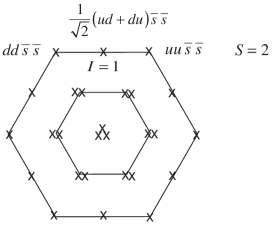
Figure 1: $SU(3)$ weight diagram for $\mathbf{27}$, where the locations of three tetraquark components of $S=2$ and $I=1$ are shown.

We have constructed five independent currents using diquark and antidiquark combination. We refer to this as the diquark construction. Similarly, we can also construct the tetraquark currents using $\bar{q}q$ combination (mesonic construction). Obviously, there are ten combinations of the Dirac ($S$, $V$, $T$, $A$ and $P$) and color ($\mathbf{1}$ and $\mathbf{8}$) spaces:

$$S_{1}=(\bar{s}_{a}u_{a})(\bar{s}_{b}d_{b})\,,~{}~{}~{}~{}~{}~{}~{}~{}~{}~{}~{}~{}~{}~{}~{}~{}~{}~{}~{}~{}~{}~{}~{}~{}~{}~{}~{}~{}S_{8}=(\bar{s}_{a}{\lambda^{n}_{ab}}u_{b})(\bar{s}_{c}{\lambda^{n}_{cd}}d_{d})\,,$$

$$V_{1}=(\bar{s}_{a}\gamma_{\mu}u_{a})(\bar{s}_{b}\gamma^{\mu}d_{b})\,,~{}~{}~{}~{}~{}~{}~{}~{}~{}~{}~{}~{}~{}~{}~{}~{}~{}~{}~{}~{}~{}~{}V_{8}=(\bar{s}_{a}\gamma_{\mu}{\lambda^{n}_{ab}}u_{b})(\bar{s}_{c}\gamma^{\mu}{\lambda^{n}_{cd}}d_{d})\,,$$

$$T_{1}=(\bar{s}_{a}\sigma_{\mu\nu}u_{a})(\bar{s}_{b}\sigma^{\mu\nu}d_{b})\,,~{}~{}~{}~{}~{}~{}~{}~{}~{}~{}~{}~{}~{}~{}~{}~{}~{}~{}~{}T_{8}=(\bar{s}_{a}\sigma_{\mu\nu}{\lambda^{n}_{ab}}u_{b})(\bar{s}_{c}\sigma^{\mu\nu}{\lambda^{n}_{cd}}d_{d})\,,$$ (7)

$$A_{1}=(\bar{s}_{a}\gamma_{\mu}\gamma_{5}u_{a})(\bar{s}_{b}\gamma^{\mu}\gamma_{5}d_{b})\,,~{}~{}~{}~{}~{}~{}~{}~{}~{}~{}~{}~{}~{}~{}~{}A_{8}=(\bar{s}_{a}\gamma_{\mu}\gamma_{5}{\lambda^{n}_{ab}}u_{b})(\bar{s}_{c}\gamma^{\mu}\gamma_{5}{\lambda^{n}_{cd}}d_{d})\,,$$

$$P_{1}=(\bar{s}_{a}\gamma_{5}u_{a})(\bar{s}_{b}\gamma_{5}d_{b})\,,~{}~{}~{}~{}~{}~{}~{}~{}~{}~{}~{}~{}~{}~{}~{}~{}~{}~{}~{}~{}~{}~{}P_{8}=(\bar{s}_{a}\gamma_{5}{\lambda^{n}_{ab}}u_{b})(\bar{s}_{c}\gamma_{5}{\lambda^{n}_{cd}}d_{d})\,,$$

where subscripts $\mathbf{1}$ and $\mathbf{8}$ denote color singlet and octet representations, respectively. Unlike the diquark construction, all the ten currents in Eq. (LABEL:define_meson_currents) remain finite. However, it is possible to show only five of them (in fact any five of them) are independent. The proof of this and various relations among different currents are discussed in Appendix. A.

III QCD Sum Rules Analysis

III.1 Formulae of QCD Sum Rule

For the past decades QCD sum rule has proven to be a very powerful and successful non-perturbative method Shifman:1978bx ; Reinders:1984sr . In sum rule analyses, we consider two-point correlation functions:

$$\Pi(q^{2})\,\equiv\,i\int d^{4}xe^{iqx}\langle 0|T\eta(x){\eta^{\dagger}}(0)|0\rangle\,,$$ (8)

where $\eta$ is an interpolating current for the tetraquark. We compute $\Pi(q^{2})$ in the operator product expansion (OPE) of QCD up to certain order in the expansion, which is then matched with a hadronic parametrization to extract information of hadron properties. At the hadron level, we express the correlation function in the form of the dispersion relation with a spectral function:

$$\Pi(p)=\int^{\infty}_{0}\frac{\rho(s)}{s-p^{2}-i\varepsilon}ds\,,$$ (9)

where

$$\rho(s) \equiv \sum_{n}\delta(s-M^{2}_{n})\langle 0|\eta|n\rangle\langle n|{\eta^{\dagger}}|0\rangle\$$ (10)

$$= f^{2}_{X}\delta(s-M^{2}_{X})+\rm{higher\,\,states}\,.$$

For the second equation, as usual, we adopt a parametrization of one pole dominance for the ground state $X$ and a continuum contribution. The sum rule analysis is then performed after the Borel transformation of the two expressions of the correlation function, (8) and (9)

$$\Pi^{(all)}(M_{B}^{2})\equiv\mathcal{B}_{M_{B}^{2}}\Pi(p^{2})=\int^{\infty}_{0}e^{-s/M_{B}^{2}}\rho(s)ds\,.$$ (11)

Assuming the contribution from the continuum states can be approximated well by the spectral density of OPE above a threshold value $s_{0}$ (duality), we arrive at the sum rule equation

$$\Pi(M_{B}^{2})\equiv f^{2}_{X}e^{-M_{X}^{2}/M_{B}^{2}}=\int^{s_{0}}_{0}e^{-s/M_{B}^{2}}\rho(s)ds\,.$$ (12)

Differentiating Eq. (12) with respect to $\frac{1}{M_{B}^{2}}$ and dividing it by Eq. (12), finally we obtain

$$M^{2}_{X}=\frac{\int^{s_{0}}_{0}e^{-s/M_{B}^{2}}s\rho(s)ds}{\int^{s_{0}}_{0}e^{-s/M_{B}^{2}}\rho(s)ds}\,.$$ (13)

In the following, we study both Eqs. (12) and (13) as functions of the parameters such as the Borel mass $M_{B}$ and the threshold value $s_{0}$ for various combinations of the tetraquark currents.

III.2 Analysis of Single Diquark Currents

In this subsection, we perform a QCD sum rule analysis using the five diquark currents, $S_{6}$, $V_{6}$, $T_{3}$, $A_{3}$ and $P_{6}$, separately. Let us first outline briefly how we performed the OPE calculation. For illustration, let us take $P_{6}$. Then

$$\Pi(q^{2})\, \equiv \,i\int d^{4}xe^{iqx}\langle 0|TP_{6}(x){P_{6}^{\dagger}}(0)|0\rangle$$

$$= Tr[C(S_{u}^{aa^{\prime}}(x))^{T}CS_{d}^{bb^{\prime}}(x)]Tr[S_{s}^{a^{\prime}a}(-x)C(S_{s}^{b^{\prime}b}(-x))^{T}C]$$

$$+Tr[C(S_{u}^{aa^{\prime}}(x))^{T}CS_{d}^{bb^{\prime}}(x)]Tr[S_{s}^{b^{\prime}a}(-x)C(S_{s}^{a^{\prime}b}(-x))^{T}C]\,.$$

For the quark propagator, we use

$$i\mbox{S}^{ab}_{q}(x) \equiv \langle 0|\mbox{T}[q^{a}(x)\bar{q}^{b}(0)]|0\rangle$$

$$= \frac{i\delta^{ab}}{2\pi^{2}x^{4}}\hat{x}+\frac{i}{32\pi^{2}}\frac{\lambda^{n}_{ab}}{2}\mbox{g}_{c}\mbox{G}^{n}_{\mu\nu}\frac{1}{x^{2}}(\sigma^{\mu\nu}\hat{x}+\hat{x}\sigma^{\mu\nu})-\frac{\delta^{ab}}{12}\langle\bar{q}q\rangle+\frac{\delta^{ab}x^{2}}{192}\langle g_{c}\bar{q}\sigma Gq\rangle$$

$$-\frac{\delta^{ab}m_{q}}{4\pi^{2}x^{2}}+\frac{i\delta^{ab}m_{q}}{48}\langle\bar{q}q\rangle\hat{x}+\frac{i\delta^{ab}m_{q}^{2}}{8\pi^{2}x^{2}}\hat{x}\,.$$

The two-point function is then divided into three parts:

1. Terms proportional to $\delta^{ab}$ ($a,b$ being color indices), where no soft gluon is emitted. The lowest term of this kind is the continuum term.

2. Terms containing one $\lambda_{ab}$ (color matrix), where one soft gluon is emitted. The lowest terms of this type contain condensates such as $\langle g\bar{q}\sigma Gq\rangle$ ($q=u$ and $d$) and $\langle g\bar{s}\sigma Gs\rangle$.

3. Terms containing two $\lambda_{ab}$’s, where two soft gluons are emitted. The lowest terms of this type contain the condensate $\langle g^{2}G^{2}\rangle$.

We have performed the OPE calculation for the spectral function up to dimension eight, which is up to the constant ($s^{0}$) term of $\rho(s)$. Actual computation is very complicated. We have performed this calculation using $Mathematica$ with $FeynCalc$ feyncalc . $Mathematica$ programs are available from the authors. The results are

$$\rho_{S6}(s) = \frac{s^{4}}{61440\pi^{6}}-\frac{{m_{s}}^{2}s^{3}}{3072\pi^{6}}+\Big{(}\frac{{m_{s}}^{4}}{256\pi^{6}}-\frac{{m_{s}}\langle\bar{s}s\rangle}{192\pi^{4}}-\frac{\langle g^{2}GG\rangle}{12288\pi^{6}}\Big{)}s^{2}$$

$$+\Big{(}-\frac{m_{s}^{3}\langle\bar{s}s\rangle}{32\pi^{4}}+\frac{m_{s}^{2}\langle g^{2}GG\rangle}{4096\pi^{6}}-\frac{m_{s}\langle g\bar{s}\sigma Gs\rangle}{64\pi^{4}}+\frac{\langle\bar{q}q\rangle^{2}}{24\pi^{2}}+\frac{\langle\bar{s}s\rangle^{2}}{24\pi^{2}}\Big{)}s$$

$$-\frac{m_{s}^{2}\langle\bar{q}q\rangle^{2}}{12\pi^{2}}+\frac{m_{s}^{2}\langle\bar{s}s\rangle^{2}}{48\pi^{2}}+\frac{\langle\bar{q}q\rangle\langle g\bar{q}\sigma Gq\rangle}{24\pi^{2}}+\frac{m_{s}\langle g^{2}GG\rangle\langle\bar{s}s\rangle}{1536\pi^{4}}+\frac{\langle\bar{s}s\rangle\langle g\bar{s}\sigma Gs\rangle}{24\pi^{2}}-\frac{m_{s}^{4}\langle g^{2}GG\rangle}{2048\pi^{6}}\,,$$

$$\rho_{V6}(s) = \frac{s^{4}}{15360\pi^{6}}-\frac{5{m_{s}}^{2}s^{3}}{1536\pi^{6}}+\Big{(}\frac{{m_{s}}^{4}}{64\pi^{6}}+\frac{{m_{s}}\langle\bar{s}s\rangle}{24\pi^{4}}+\frac{5\langle g^{2}GG\rangle}{6144\pi^{6}}\Big{)}s^{2}$$

$$+\Big{(}-\frac{m_{s}^{3}\langle\bar{s}s\rangle}{8\pi^{4}}-\frac{11m_{s}^{2}\langle g^{2}GG\rangle}{2048\pi^{6}}+\frac{m_{s}\langle g\bar{s}\sigma Gs\rangle}{32\pi^{4}}-\frac{\langle\bar{q}q\rangle^{2}}{12\pi^{2}}-\frac{\langle\bar{s}s\rangle^{2}}{12\pi^{2}}\Big{)}s$$

$$+\frac{2m_{s}^{2}\langle\bar{q}q\rangle^{2}}{3\pi^{2}}+\frac{m_{s}^{2}\langle\bar{s}s\rangle^{2}}{12\pi^{2}}-\frac{\langle\bar{q}q\rangle\langle g\bar{q}\sigma Gq\rangle}{12\pi^{2}}+\frac{7m_{s}\langle g^{2}GG\rangle\langle\bar{s}s\rangle}{768\pi^{4}}-\frac{\langle\bar{s}s\rangle\langle g\bar{s}\sigma Gs\rangle}{12\pi^{2}}\,,$$

$$\rho_{T3}(s) = \frac{s^{4}}{5120\pi^{6}}-\frac{{m_{s}}^{2}s^{3}}{128\pi^{6}}+\Big{(}\frac{3{m_{s}}^{4}}{64\pi^{6}}+\frac{{m_{s}}\langle\bar{s}s\rangle}{16\pi^{4}}+\frac{\langle g^{2}GG\rangle}{1536\pi^{6}}\Big{)}s^{2}+\Big{(}-\frac{3m_{s}^{3}\langle\bar{s}s\rangle}{8\pi^{4}}-\frac{m_{s}^{2}\langle g^{2}GG\rangle}{256\pi^{6}}\Big{)}s$$ (18)

$$+\frac{m_{s}^{2}\langle\bar{q}q\rangle^{2}}{\pi^{2}}+\frac{m_{s}^{2}\langle\bar{s}s\rangle^{2}}{4\pi^{2}}+\frac{m_{s}\langle g^{2}GG\rangle\langle\bar{s}s\rangle}{192\pi^{4}}-\frac{m_{s}^{4}\langle g^{2}GG\rangle}{256\pi^{6}}\,,$$

$$\rho_{A3}(s) = \frac{s^{4}}{30720\pi^{6}}-\frac{{m_{s}}^{2}s^{3}}{1024\pi^{6}}+\Big{(}\frac{{m_{s}}^{4}}{128\pi^{6}}+\frac{\langle g^{2}GG\rangle}{6144\pi^{6}}\Big{)}s^{2}$$

$$+\Big{(}-\frac{m_{s}^{3}\langle\bar{s}s\rangle}{16\pi^{4}}-\frac{3m_{s}^{2}\langle g^{2}GG\rangle}{2048\pi^{6}}-\frac{m_{s}\langle g\bar{s}\sigma Gs\rangle}{64\pi^{4}}+\frac{\langle\bar{q}q\rangle^{2}}{24\pi^{2}}+\frac{\langle\bar{s}s\rangle^{2}}{24\pi^{2}}\Big{)}s$$

$$+\frac{m_{s}^{2}\langle\bar{s}s\rangle^{2}}{24\pi^{2}}+\frac{\langle\bar{q}q\rangle\langle g\bar{q}\sigma Gq\rangle}{24\pi^{2}}+\frac{m_{s}\langle g^{2}GG\rangle\langle\bar{s}s\rangle}{256\pi^{4}}+\frac{\langle\bar{s}s\rangle\langle g\bar{s}\sigma Gs\rangle}{24\pi^{2}}\,,$$

$$\rho_{P6}(s) = \frac{s^{4}}{61440\pi^{6}}-\frac{{m_{s}}^{2}s^{3}}{1024\pi^{6}}+\Big{(}\frac{{m_{s}}^{4}}{256\pi^{6}}-\frac{{m_{s}}\langle\bar{s}s\rangle}{64\pi^{4}}-\frac{\langle g^{2}GG\rangle}{12288\pi^{6}}\Big{)}s^{2}$$

$$+\Big{(}-\frac{m_{s}^{3}\langle\bar{s}s\rangle}{32\pi^{4}}+\frac{3m_{s}^{2}\langle g^{2}GG\rangle}{4096\pi^{6}}+\frac{m_{s}\langle g\bar{s}\sigma Gs\rangle}{64\pi^{4}}-\frac{\langle\bar{q}q\rangle^{2}}{24\pi^{2}}-\frac{\langle\bar{s}s\rangle^{2}}{24\pi^{2}}\Big{)}s$$

$$+\frac{m_{s}^{2}\langle\bar{q}q\rangle^{2}}{4\pi^{2}}+\frac{m_{s}^{2}\langle\bar{s}s\rangle^{2}}{48\pi^{2}}-\frac{\langle\bar{q}q\rangle\langle g\bar{q}\sigma Gq\rangle}{24\pi^{2}}-\frac{m_{s}\langle g^{2}GG\rangle\langle\bar{s}s\rangle}{512\pi^{4}}-\frac{\langle\bar{s}s\rangle\langle g\bar{s}\sigma Gs\rangle}{24\pi^{2}}-\frac{m_{s}^{4}\langle g^{2}GG\rangle}{2048\pi^{6}}\,.$$

In these equations, $q$ represents a $u$ or $d$ quark, and $s$ represents an $s$ quark. $\langle\bar{q}q\rangle$ and $\langle\bar{s}s\rangle$ are dimension $D=3$ quark condensates; $\langle g^{2}GG\rangle$ is a $D=4$ gluon condensate; $\langle g\bar{q}\sigma Gq\rangle$ and $\langle g\bar{s}\sigma Gs\rangle$ are $D=5$ mixed condensates. From these expressions, we observe the followings:

• The coefficients of the lowest dimension, or of the leading term in powers of $s$, have the relations $c_{S6}^{(4)}=c_{P3}^{(4)}$ and $c_{A3}^{(4)}=1/2c_{V6}^{(4)}$. These are the consequences of chiral symmetry at the perturbative level Hosaka:2001ux .

• As empirically known, the terms of quark condensates have important contributions to the sum rule.

For numerical calculations, we use the following values of condensatesYang:1993bp ; Narison:2002pw ; Gimenez:2005nt ; Jamin:2002ev ; Ioffe:2002be ; Ovchinnikov:1988gk ; Eidelman:2004wy :

$$\langle\bar{q}q\rangle=-(0.240\mbox{ GeV})^{3}\,,$$

$$\langle\bar{s}s\rangle=-(0.8\pm 0.1)\times(0.240\mbox{ GeV})^{3}\,,$$

$$\langle g_{s}^{2}GG\rangle=(0.48\pm 0.14)\mbox{ GeV}^{4}\,,$$

$$m_{s}(2\mbox{ GeV})=0.11\mbox{ GeV}\,,$$ (21)

$$\langle g_{s}\bar{q}\sigma Gq\rangle=-M_{0}^{2}\times\langle\bar{q}q\rangle\,,$$

$$M_{0}^{2}=(0.8\pm 0.2)\mbox{ GeV}^{2}\,.$$

As usual we assume the vacuum saturation for higher dimensional operators such as $\langle 0|\bar{q}q\bar{q}q|0\rangle\sim\langle 0|\bar{q}q|0\rangle\langle 0|\bar{q}q|0\rangle$. There is a minus sign in the definition of the mixed condensate $\langle g_{s}\bar{q}\sigma Gq\rangle$, which is different with some other QCD sum rule calculation. This is just because the definition of coupling constant $g_{s}$ is different Yang:1993bp ; Hwang:1994vp .

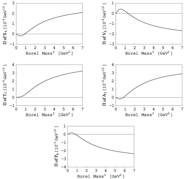
Figure 2: Borel transformed correlation functions $\Pi_{S6}$, $\Pi_{V6}$, $\Pi_{T3}$, $\Pi_{A3}$ and $\Pi_{P6}$ as functions of Borel mass square, in units of $\mbox{GeV}^{10}$, for threshold value $s_{0}=3$ GeV².

In Fig. 2, we show all five Borel transformed correlation functions $\Pi(M_{B}^{2})$ (the LHS of the Eq. (12)) as functions of Borel mass square for threshold value $s_{0}=3$ GeV². From the definition of (10), the LHS should be positive definite quantities. In practical calculations, however, the positivity may not be necessarily realized, if the OPE up to finite terms does not work due to insufficient convergence of the OPE. In the present analysis, we find that among the five cases, two functions of $V_{6}$ and $P_{6}$ currents show such a bad behavior. Therefore, the QCD sum rules for these two currents are not physically acceptable. The correlation functions of $A_{3}$ and $S_{6}$ change the sign from negative to positive values. But the sum rule values take positive values for $M_{B}^{2}\sim$ several GeV².

The tetraquark currents $S_{6}$ and $A_{3}$ are constructed by diquark fields which correspond to ${}^{1}S_{0}$ and ${}^{3}S_{1}$ in the non-relativistic language, where the two quarks can be in the ground state $s$-orbit. In contrast, the currents $V_{6}$ and $P_{6}$ correspond to linear combinations of ${}^{3}P_{1}$, and ${}^{3}P_{0}$, respectively, where one of the two quarks is in an excited $p$-orbit. The $T_{3}$ current is a linear combination of ${}^{3}S_{1}$ and ${}^{1}P_{1}$. Therefore, we verify an empirical fact that the sum rule constructed by currents having the $s$-wave components in the non-relativistic limit works better than those dominated by $p$-wave components. For completeness, we show the LHS with numerical coefficients for the three better cases: $A_{3}$, $T_{3}$ and $S_{6}$

$$\Pi_{A3}^{(all)} = 8.2\times 10^{-7}M_{B}^{10}-7.4\times 10^{-8}M_{B}^{8}+1.6\times 10^{-7}M_{B}^{6}+1.8\times 10^{-6}M_{B}^{4}-1.1\times 10^{-6}M_{B}^{2}\,,$$

$$\Pi_{T3}^{(all)} = 4.8\times 10^{-6}M_{B}^{10}-5.9\times 10^{-7}M_{B}^{8}-9.1\times 10^{-7}M_{B}^{6}+3.4\times 10^{-8}M_{B}^{4}+2.4\times 10^{-7}M_{B}^{2}\,,$$

$$\Pi_{S6}^{(all)} = 4.1\times 10^{-7}M_{B}^{10}-2.5\times 10^{-8}M_{B}^{8}+5.1\times 10^{-8}M_{B}^{6}+1.8\times 10^{-6}M_{B}^{4}-1.1\times 10^{-6}M_{B}^{2}\,.$$

From these expressions, we observe that the convergence of the current $T_{3}$ seems better, while the convergence of the currents $A_{3}$ and $S_{6}$ is not very good in the region $1<M_{B}^{2}<2$ GeV². They can only converge at $M_{B}^{2}\sim 3$ GeV².

To determine the mass, we need to fix the two parameters: the threshold value $s_{0}$ and the Borel mass square $M_{B}^{2}$. For a good sum rule, the predicted masses should not depend on these two parameters strongly with sizable pole contribution (Borel window). In Fig. 3, we show the masses of the tetraquark as functions of the Borel mass for several threshold values $s_{0}$ (Borel curves). We observe that the Borel mass dependence is somewhat strong for the currents $S_{6}$ and $A_{3}$ in the region $1<M_{B}^{2}<2$ GeV², which is expected to be a reasonable choice of the Borel mass. For these currents $S_{6}$ and $A_{3}$, however, we see that the minimum occurs at around 3 GeV² when $s_{0}$ is varied in the region $M_{B}^{2}\ \raise 1.29167pt\hbox{$>$\kern-7.5pt\lower 4.30554pt\hbox{$\sim$}}\ 1.5$ GeV². (For the current $S_{6}$, the mass of $s_{0}=2$ GeV² is far above the region shown in the figure.) For this reason, we consider that $s_{0}=3$ GeV² is a reasonable choice which we will mainly use for the estimation of the mass of the tetraquark in the following sum rule analyses. At this $s_{0}$ value, the mass of the tetraquark turns out to be about 1.6 GeV. For the $T_{3}$ current, the Borel stability seems better. The result, however, depends on the threshold value $s_{0}$ to some extent. However, it is interesting to see that the mass of the tetraquark is about 1.6 GeV when $s_{0}\sim 3$ GeV².

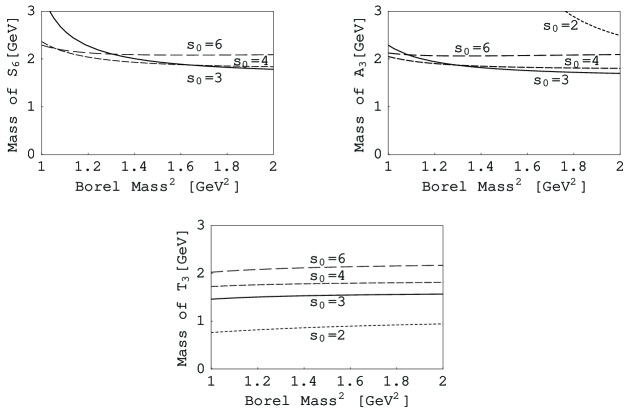
Figure 3: Mass of the tetraquark calculated by the three currents $S_{6}$, $A_{3}$ and $T_{3}$, as functions of the Borel mass square $M_{B}^{2}$, for several threshold values $s_{0}=2,3,4$ and 6 GeV².

To see the amount of the pole contribution, we define the quantity

$$\mbox{Pole contribution}\equiv\frac{\int_{4m_{s}^{2}}^{s_{0}}e^{-s/M_{B}^{2}}\rho(s)ds}{\int_{4m_{s}^{2}}^{\infty}e^{-s/M_{B}^{2}}\rho(s)ds}\,.$$ (23)

As shown in Table 1, the pole contribution of the diquark currents $A_{3}$, $T_{3}$ and $S_{6}$ are not very large; at $M_{B}^{2}\sim 1$ GeV² they are of order 10 %. This is a general problem of the QCD sum rule when multi-quark currents are used. Therefore the results so far might be doubtful.

Table 1: Pole contributions of various currents. The threshold value $s_{0}=3$ GeV² is used.

	Diquark Current			Mesonic Current		Mixed Current
$M_{B}^{2}$	$A_{3}$	$T_{3}$	$S_{6}$	$V_{8}$	$T_{8}$	$\eta_{1}$	$\eta_{2}$
0.7 GeV2	—	—	—	—	—	0.60	0.49
1 GeV2	0.17	0.11	0.10	0.54	0.23	0.30	0.22
2 GeV2	0.04	0.01	0.05	0.09	0.02	0.03	0.02

From the analysis of the single current of the diquark construction, we expect that the mass of the tetraquark is about 1.6 GeV, although the stability against the variation of both the Borel mass and the threshold parameter is not simultaneously achieved. Furthermore, the pole contribution is rather small. As we will see, however, a suitable linear combination will improve them.

III.3 Analysis of Single Mesonic Currents

In this subsection, we perform QCD sum rule analysis using the ten mesonic currents, $S_{1,8}$, $V_{1,8}$, $T_{1,8}$, $A_{1,8}$ and $P_{1,8}$, separately. Here we only show two important spectral densities:

$$\rho_{V8}(s) = \frac{s^{4}}{110592\pi^{6}}-\frac{19{m_{s}}^{2}s^{3}}{55296\pi^{6}}+\Big{(}\frac{5{m_{s}}^{4}}{2304\pi^{6}}-\frac{{m_{s}}\langle\bar{q}q\rangle}{432\pi^{4}}+\frac{{m_{s}}\langle\bar{s}s\rangle}{432\pi^{4}}+\frac{17\langle g^{2}GG\rangle}{221184\pi^{6}}\Big{)}s^{2}$$

$$+\Big{(}\frac{m_{s}^{3}\langle\bar{q}q\rangle}{72\pi^{4}}-\frac{5m_{s}^{3}\langle\bar{s}s\rangle}{288\pi^{4}}-\frac{13m_{s}^{2}\langle g^{2}GG\rangle}{24576\pi^{6}}+\frac{m_{s}\langle g\bar{q}Gq\rangle}{2304\pi^{4}}-\frac{5m_{s}\langle g\bar{s}Gs\rangle}{4608\pi^{4}}$$

$$+\frac{\langle\bar{q}q\rangle^{2}}{432\pi^{2}}+\frac{\langle\bar{s}s\rangle^{2}}{432\pi^{2}}+\frac{\langle\bar{q}q\rangle\langle\bar{s}s\rangle}{54\pi^{2}}\Big{)}s+\frac{m_{s}^{2}\langle\bar{q}q\rangle^{2}}{27\pi^{2}}+\frac{5m_{s}^{2}\langle\bar{s}s\rangle^{2}}{432\pi^{2}}$$

$$-\frac{m_{s}\langle\bar{q}q\rangle\langle g^{2}GG\rangle}{6912\pi^{4}}+\frac{5\langle\bar{q}q\rangle\langle g\bar{q}Gq\rangle}{1728\pi^{2}}+\frac{m_{s}^{3}\langle g\bar{q}Gq\rangle}{144\pi^{4}}-\frac{m_{s}^{2}\langle\bar{q}q\rangle\langle\bar{s}s\rangle}{18\pi^{2}}-\frac{\langle g\bar{q}Gq\rangle\langle\bar{s}s\rangle}{864\pi^{2}}$$

$$+\frac{m_{s}\langle g^{2}GG\rangle\langle\bar{s}s\rangle}{1024\pi^{4}}-\frac{\langle\bar{q}q\rangle\langle g\bar{s}Gs\rangle}{864\pi^{2}}+\frac{5\langle\bar{s}s\rangle\langle g\bar{s}Gs\rangle}{1728\pi^{2}}-\frac{m_{s}^{4}\langle g^{2}GG\rangle}{9216\pi^{6}}\,,$$

$$\rho_{T8}(s) = \frac{s^{4}}{18432\pi^{6}}-\frac{5{m_{s}}^{2}s^{3}}{2304\pi^{6}}+\Big{(}\frac{5{m_{s}}^{4}}{384\pi^{6}}+\frac{5{m_{s}}\langle\bar{s}s\rangle}{288\pi^{4}}+\frac{31\langle g^{2}GG\rangle}{55296\pi^{6}}\Big{)}s^{2}$$

$$+\Big{(}-\frac{5m_{s}^{3}\langle\bar{s}s\rangle}{48\pi^{4}}-\frac{31m_{s}^{2}\langle g^{2}GG\rangle}{9216\pi^{6}}\Big{)}s+\frac{5m_{s}^{2}\langle\bar{q}q\rangle^{2}}{18\pi^{2}}+\frac{5m_{s}^{2}\langle\bar{s}s\rangle^{2}}{72\pi^{2}}$$

$$+\frac{31m_{s}\langle g^{2}GG\rangle\langle\bar{s}s\rangle}{6912\pi^{4}}-\frac{13m_{s}^{4}\langle g^{2}GG\rangle}{9216\pi^{6}}\,.$$

As shown in Fig. 4, we find that among the ten correlation functions, only two correlation functions for the currents $V_{8}$ and $T_{8}$ show good behavior with having positive values.

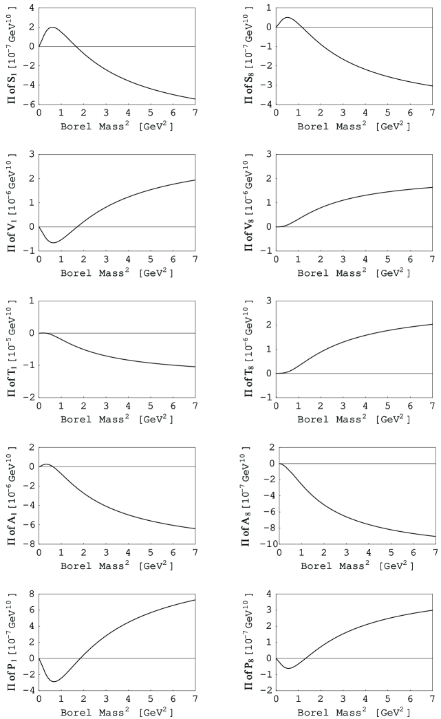
Figure 4: Borel transformed correlation functions $\Pi_{S1}$, $\Pi_{S8}$, $\Pi_{V1}$, $\Pi_{V8}$, $\Pi_{T1}$, $\Pi_{T8}$, $\Pi_{A1}$, $\Pi_{A8}$, $\Pi_{P1}$ and $\Pi_{P8}$ as functions of Borel mass square, in units of $\mbox{GeV}^{10}$, for threshold value $s_{0}=3$ GeV².

The currents $V_{1}$, $V_{8}$, $P_{1}$ and $P_{8}$ are constructed by mesonic fields (either color singlet or color octet) which correspond to ${}^{3}S_{1}$ and ${}^{1}S_{0}$ in the non-relativistic language, where two quark-antiquark pairs can be in the ground state $s$-orbit. Their spectral densities then show similar behavior to $S_{6}$ and $A_{3}$ in the previous subsection. In contrast, $S_{1}$, $S_{8}$, $A_{1}$ and $A_{8}$ correspond to linear combinations of ${}^{3}P_{0}$ and ${}^{3}P_{1}$, respectively; $T_{1}$ and $T_{8}$ currents are the combinations of ${}^{3}S_{1}$ and ${}^{1}P_{1}$.

From the above argument, we might expect that six currents, $V_{1}$, $V_{8}$, $P_{1}$, $P_{8}$, $T_{1}$ and $T_{8}$ would work. However, we found that the Borel transformed correlation functions calculated by the currents $V_{1}$, $P_{1}$, $P_{8}$ and $T_{1}$ take negative values and therefore, they must be abandoned. Now there remain only two better currents $V_{8}$ and $T_{8}$ in the mesonic construction. This is the reason why we have shown their spectral densities in (III.3) and (III.3). Using the numerical values of various condensates (21), we find the Borel transformed correlation functions

$$\Pi_{V8}^{(all)} = 2.3\times 10^{-7}M_{B}^{10}-2.6\times 10^{-8}M_{B}^{8}+9.1\times 10^{-8}M_{B}^{6}+3.5\times 10^{-7}M_{B}^{4}-4.9\times 10^{-8}M_{B}^{2}\,,$$

$$\Pi_{T8}^{(all)} = 1.4\times 10^{-6}M_{B}^{10}-1.7\times 10^{-7}M_{B}^{8}+1.2\times 10^{-7}M_{B}^{6}-4.3\times 10^{-9}M_{B}^{4}+4.9\times 10^{-8}M_{B}^{2}\,.$$

From these equations, we find that better convergence is achieved for $T_{8}$ than for $V_{8}$ in the region $1\lesssim M_{B}^{2}\lesssim 2$ GeV². The pole contributions are significantly improved as shown in Table 1.

In Fig. 5, we show the masses of the tetraquark currents $V_{8}$ and $T_{8}$ as functions of the Borel mass for several threshold values $s_{0}$ (Borel curves). As in the case of $T_{3}$ current, the Borel stability seems good but the result depends on the threshold value $s_{0}$. However, once again, if we take the threshold value at $s_{0}\sim 3$ GeV², the mass of the tetraquark turns out to be reasonable, though the precise values are slightly smaller: the mass of $T_{8}\sim 1.5$ GeV and the mass of $V_{8}\sim 1.4$ GeV.

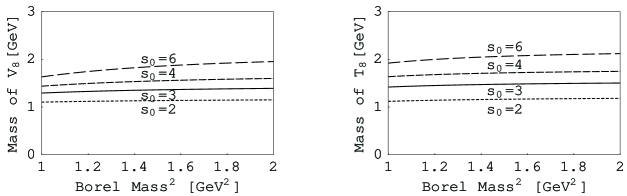
Figure 5: Mass of the tetraquark calculated by the currents $V_{8}$(Left) and $T_{8}$(Right), as functions of the Borel mass square $M_{B}^{2}$, for several threshold values $s_{0}=2,3,4$ and 6 GeV².

III.4 Analysis of Mixed Currents

In order to improve the sum rule, we attempt to make linear combinations of independent currents for both diquark and mesonic currents. Since linear combinations of five currents contain ten mixing angles, the full consideration with these ten parameters is rather cumbersome. Instead, we make a linear combination of two currents $J_{1}$ and $J_{2}$ (any two from the independent currents), $\eta=\cos\theta J_{1}+\sin\theta J_{2}$, where $\theta$ is a mixing angle. Then the correlation functions are written as

$$\langle\eta\eta^{\dagger}\rangle=\cos^{2}\theta\langle J_{1}J_{1}^{\dagger}\rangle+\sin^{2}\theta\langle J_{2}J_{2}^{\dagger}\rangle+\cos\theta\sin\theta\langle J_{1}J_{2}^{\dagger}\rangle+\cos\theta\sin\theta\langle J_{2}J_{1}^{\dagger}\rangle\,.$$ (27)

The mixing is chosen with the following requirements:

1. The OPE has a good convergence as going to terms of higher dimensional operators.

2. The spectral density becomes positive for all (or almost all) $s$ values, and then $\Pi(M_{B}^{2})$ becomes positive for all Borel mass and threshold values.

3. Pole contribution is sufficiently large.

We have tried various combinations of two currents to realize good sum rules. While doing so, we have realized that the diquark currents are more independent than the mesonic currents. This means that the cross terms of (27) have only a minor contribution for diquark currents, while they have a large contribution for mesonic currents.

According to the requirement (1), we would like to make a linear combination such that the highest dimensional (eight) term is suppressed. For diquark currents, we find it convenient to take two combinations:

$$\eta = \cos\theta A_{3}+\sin\theta V_{6}\,,$$ (28)

$$\xi = \cos\theta P_{6}+\sin\theta S_{6}\,.$$ (29)

By choosing $\cot\theta\sim\sqrt{2}$, we find that the term of dimension eight of (28) is suppressed, while for $\cot\theta\sim 1$, the term of dimension eight of (29) is suppressed. The Borel transformed correlation function of (29) $\Pi_{\xi}(M_{B}^{2})$, however, takes negative values. Therefore, this current should be rejected for the sum rule analysis. In this way we are led to the current $\eta$ of (28). From now on, we will denote $\eta\to\eta_{1}$.

For the mesonic case, it turns out that the cross term contributions are large. Accordingly, we attempt a complex angle to improve the sum rule analysis. By choosing $t_{1}=0.91,~{}t_{2}=-0.41$, we construct a current:

$$\eta_{2} = S_{1}+(t_{1}+\mathbf{i}t_{2})P_{1}\,.$$ (30)

The numerical Borel transformed correlation functions are

$$\Pi_{1}^{(all)} = 1.1\times 10^{-6}M_{B}^{10}-1.3\times 10^{-7}M_{B}^{8}+4.8\times 10^{-7}M_{B}^{6}-2.0\times 10^{-8}M_{B}^{4}+5.2\times 10^{-9}M_{B}^{2}\,,$$

$$\Pi_{2}^{(all)} = 5.0\times 10^{-7}M_{B}^{10}-6.0\times 10^{-8}M_{B}^{8}+8.4\times 10^{-8}M_{B}^{6}-2.2\times 10^{-8}M_{B}^{4}+8.3\times 10^{-9}M_{B}^{2}\,,$$

which may be compared with the previous results of (III.2) and (III.3). It looks that the convergence of the series is improved significantly. Therefore, we can choose a smaller Borel mass square down to $M_{B}^{2}\gtrsim 0.7$ GeV², where the pole contribution will be further increased up to around 50 %, and the convergence is still maintained.

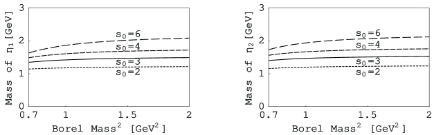
Figure 6: Mass of the tetraquark calculated by the mixed currents $\eta_{1}$(Left) and $\eta_{2}$(Right), as functions of the Borel mass square $M_{B}^{2}$ for several threshold values $s_{0}=2,3,4$ and 6 GeV².

In Fig. 6, we show the mass calculated from $\eta_{1}$ and $\eta_{2}$ as functions of the Borel mass square for several threshold values $s_{0}$. The Borel stability is improved from the cases of the single currents. From these figures, we might think that there is still a substantial $s_{0}$ dependence. However, this dependence will be largely reduced if we choose a small Borel mass, where the pole contribution is sufficiently large. In Fig. 7, we show the mass calculated from $\eta_{1}$ and $\eta_{2}$ as functions of the threshold value for several Borel masses. When $M_{B}^{2}=0.7$ GeV², the curve is very stable. Moreover, the pole contribution is around 50 %, and the convergence is still maintained. Therefore, we obtain a very good sum rule, where we find the mass calculated from the two currents $\eta_{1}$ and $\eta_{2}$ is about 1.5 GeV. As the Borel mass increases, the pole contribution decreases, and accordingly, the threshold dependence becomes bigger.

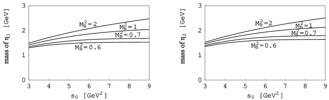
Figure 7: Mass of the tetraquark calculated by the mixed currents $\eta_{1}$(Left) and $\eta_{2}$(Right), as functions of the threshold value $s_{0}$ for several Borel mass square $M_{B}^{2}=0.6,0.7,1$ and 2 GeV².

Finally, in order to summarize our analysis, we show in Fig. 8 masses of the tetraquark calculated by several reasonable currents used in the present study as functions of the Borel mass square at $s_{0}=3$ GeV². They are $S_{6}$, $A_{3}$ and $T_{3}$ for the diquark construction, $T_{8}$ and $V_{8}$ for the mesonic construction, and $\eta_{1}$ and $\eta_{2}$ for the mixed currents. The plots are extended to a wider region of $M_{B}^{2}$ up to 4 GeV², where the masses predicted by different currents tend to a same value. We verify once again a good Borel mass stability for the mixed currents, while some of the single currents show good stability also ($T_{3},T_{8}$ and $V_{8}$). The mass values varies slightly, while we expect the mass of the tetraquark around 1.5 GeV.

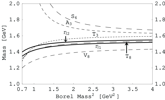
Figure 8: Mass of the tetraquark calculated by the currents $\eta_{1}$, $\eta_{2}$, $A_{3}$, $S_{6}$, $T_{3}$, $V_{8}$ and $T_{8}$, as functions of the Borel mass square $M_{B}^{2}$ in the region $0.7<M_{B}^{2}<4$ GeV², for threshold value $s_{0}=3$ GeV².

IV Summary

We have presented a QCD sum rule study of the $ud\bar{s}\bar{s}$ tetraquark of $J^{P}=0^{+}$ and $I=1$, both in the diquark ($(\bar{q}\bar{q})(qq)$) and mesonic ($(\bar{q}q)(\bar{q}q)$) constructions. We have found that in this channel of tetraquark, there are five independent currents, which is shown both in the diquark and mesonic constructions. For each single current, we have tested the sum rule analysis, but it is found that not all of them provide a good stability.

As an attempt to improve the stability of the sum rule, we have considered linear combinations of independent currents. In order to simplify the analysis, we took a superposition of various combinations of two currents. Among them, we have found two cases that lead to good sum rules, where we investigated $s_{0}$ (threshold value) and $M_{B}$ (Borel mass) dependence, and convergence of OPE. A good Borel stability is achieved in the region $0.7\ \raise 1.29167pt\hbox{$<$\kern-7.5pt\lower 4.30554pt\hbox{$\sim$}}\ M_{B}^{2}\ \raise 1.29167pt\hbox{$<$\kern-7.5pt\lower 4.30554pt\hbox{$\sim$}}\ 4$ GeV². In order to obtain a large enough pole contribution (50 %) and reduce the threshold value dependence, we have to reduce the Borel mass. However, to maintain the convergence of OPE, we can not reduce it too largely. When Borel mass square $M_{B}^{2}$ is around 0.7 GeV², we get a very good QCD sum rule, where the mass of the tetraquark turns out to be around 1.5 GeV.

Despite the seemingly good Borel mass stability, we think that we should investigate the following points more carefully. For instance, estimation of higher dimensional terms of ${\cal O}(1/s)$ could be important. Although we are able to construct the two mixed currents such that the higher order contributions (in the present calculation of OPE) of dimension six and eight terms are suppressed, the question still remains concerning even higher order contributions. Another question is the contribution of $KK$ scattering states, since the mass of the tetraquark is around $1.5$ GeV, and it can fall apart into the $KK$ states. Such a contribution can be estimated by using the method proposed in Refs. Lee:2004xk ; Kwon:2005fe . These will be further investigated in the future work.

Appendix A Five Independent Currents in $(\bar{q}q)(\bar{q}q)$ Basis

We attempt to write a diquark current of (LABEL:define_diquark_current) as a sum of $(\bar{q}q)$ mesonic pairs ($q=u,d,s)$,

$$L_{\mu\nu\rho\sigma}\times\bar{s}_{a}^{\mu}\bar{s}_{b}^{\nu}u_{c}^{\rho}d_{d}^{\sigma}=\sum_{n,i,j}C_{i}^{1}C_{j}^{2}(\bar{s}_{b}\lambda^{n}\Gamma_{i}d_{d})(\bar{s}_{a}\lambda^{n}\Gamma_{j}u_{c})\,,$$ (32)

where $\Gamma_{i}$ are the five Dirac matrices and $\lambda^{n}(n=1,\cdots,8)$ are color matrices forming color singlet and octet states out of $\mathbf{3}\times\mathbf{\bar{3}}$. Therefore, in (32), the sum runs over ten terms of five $\Gamma_{i}$ matrices and two $\lambda^{n}$ combinations. They are

$$S_{1}=(\bar{s}_{a}u_{a})(\bar{s}_{b}d_{b})\,,~{}~{}~{}~{}~{}~{}~{}~{}~{}~{}~{}~{}~{}~{}~{}~{}~{}~{}~{}~{}~{}~{}~{}~{}~{}~{}~{}~{}S_{8}=(\bar{s}_{a}{\lambda^{n}_{ab}}u_{b})(\bar{s}_{c}{\lambda^{n}_{cd}}d_{d})\,,$$

$$V_{1}=(\bar{s}_{a}\gamma_{\mu}u_{a})(\bar{s}_{b}\gamma^{\mu}d_{b})\,,~{}~{}~{}~{}~{}~{}~{}~{}~{}~{}~{}~{}~{}~{}~{}~{}~{}~{}~{}~{}~{}~{}V_{8}=(\bar{s}_{a}\gamma_{\mu}{\lambda^{n}_{ab}}u_{b})(\bar{s}_{c}\gamma^{\mu}{\lambda^{n}_{cd}}d_{d})\,,$$

$$T_{1}=(\bar{s}_{a}\sigma_{\mu\nu}u_{a})(\bar{s}_{b}\sigma^{\mu\nu}d_{b})\,,~{}~{}~{}~{}~{}~{}~{}~{}~{}~{}~{}~{}~{}~{}~{}~{}~{}~{}~{}T_{8}=(\bar{s}_{a}\sigma_{\mu\nu}{\lambda^{n}_{ab}}u_{b})(\bar{s}_{c}\sigma^{\mu\nu}{\lambda^{n}_{cd}}d_{d})\,,$$ (33)

$$A_{1}=(\bar{s}_{a}\gamma_{\mu}\gamma_{5}u_{a})(\bar{s}_{b}\gamma^{\mu}\gamma_{5}d_{b})\,,~{}~{}~{}~{}~{}~{}~{}~{}~{}~{}~{}~{}~{}~{}~{}A_{8}=(\bar{s}_{a}\gamma_{\mu}\gamma_{5}{\lambda^{n}_{ab}}u_{b})(\bar{s}_{c}\gamma^{\mu}\gamma_{5}{\lambda^{n}_{cd}}d_{d})\,,$$

$$P_{1}=(\bar{s}_{a}\gamma_{5}u_{a})(\bar{s}_{b}\gamma_{5}d_{b})\,,~{}~{}~{}~{}~{}~{}~{}~{}~{}~{}~{}~{}~{}~{}~{}~{}~{}~{}~{}~{}~{}~{}P_{8}=(\bar{s}_{a}\gamma_{5}{\lambda^{n}_{ab}}u_{b})(\bar{s}_{c}\gamma_{5}{\lambda^{n}_{cd}}d_{d})\,,$$

where in the octet representation inner product of $\lambda^{n}$ ($n=1,\cdots,8$) is taken. The quark-antiquark pairs in different currents have different properties:

$$S_{1}:(J^{P}=0^{+},8_{f},1_{c}),~{}~{}~{}~{}~{}~{}~{}~{}~{}~{}~{}~{}~{}~{}~{}~{}~{}S_{8}:(J^{P}=0^{+},8_{f},8_{c}),$$

$$V_{1}:(J^{P}=1^{-},8_{f},1_{c}),~{}~{}~{}~{}~{}~{}~{}~{}~{}~{}~{}~{}~{}~{}~{}~{}~{}V_{8}:(J^{P}=1^{-},8_{f},8_{c}),$$

$$T_{1}:(J^{P}=1^{+}\&1^{-},8_{f},1_{c}),~{}~{}~{}~{}~{}~{}~{}~{}~{}~{}~{}T_{8}:(J^{P}=1^{+}\&1^{-},8_{f},8_{c}),$$

$$A_{1}:(J^{P}=1^{+},8_{f},1_{c}),~{}~{}~{}~{}~{}~{}~{}~{}~{}~{}~{}~{}~{}~{}~{}~{}A_{8}:(J^{P}=1^{+},8_{f},8_{c}),$$

$$P_{1}:(J^{P}=0^{-},8_{f},1_{c}),~{}~{}~{}~{}~{}~{}~{}~{}~{}~{}~{}~{}~{}~{}~{}~{}~{}P_{8}:(J^{P}=0^{-},8_{f},8_{c}).$$

In order to establish the five independent currents, first we change their color structures

$$(\bar{s}_{a}u_{b})(\bar{s}_{b}d_{a})=\frac{1}{3}(\bar{s}_{a}u_{a})(\bar{s}_{b}d_{b})+\frac{1}{2}(\bar{s}_{a}u_{b})(\bar{s}_{c}d_{d}){\lambda_{ab}}{\lambda_{cd}}\,,$$

$$(\bar{s}_{a}u_{d})(\bar{s}_{c}d_{b}){\lambda_{ab}}{\lambda_{cd}}=\frac{16}{9}(\bar{s}_{a}u_{a})(\bar{s}_{b}d_{b})-\frac{1}{3}(\bar{s}_{a}u_{b})(\bar{s}_{c}d_{d}){\lambda_{ab}}{\lambda_{cd}}\,.$$ (34)

Then we use the Fierz transformation Maruhn:2000af

$$\frac{1}{3}(\bar{s}_{a}u_{a})(\bar{s}_{b}d_{b})+\frac{1}{2}(\bar{s}_{a}u_{b})(\bar{s}_{c}d_{d}){\lambda_{ab}}{\lambda_{cd}}$$

$$= (\bar{s}_{a}u_{b})(\bar{s}_{b}d_{a})$$ (35)

$$= -\frac{1}{4}\{(\bar{s}_{a}u_{a})(\bar{s}_{b}d_{b})+(\bar{s}_{a}\gamma_{\mu}u_{a})(\bar{s}_{b}\gamma^{\mu}d_{b})+\frac{1}{2}(\bar{s}_{a}\sigma_{\mu\nu}u_{a})(\bar{s}_{b}\sigma^{\mu\nu}d_{b})$$

$$-(\bar{s}_{a}\gamma_{\mu}{}\gamma_{5}u_{a})(\bar{s}_{b}\gamma^{\mu}{}\gamma_{5}d_{b})+(\bar{s}_{a}\gamma_{5}u_{a})(\bar{s}_{b}\gamma_{5}d_{b})\}\,.$$

We obtain 10 equations in all

$$\frac{1}{3}S_{1}+\frac{1}{2}S_{8}=-\frac{1}{4}\{S_{1}+V_{1}+\frac{1}{2}T_{1}-A_{1}+P_{1}\}\,,$$

$$\frac{16}{9}S_{1}-\frac{1}{3}S_{8}=-\frac{1}{4}\{S_{8}+V_{8}+\frac{1}{2}T_{8}-A_{8}+P_{8}\}\,,$$

$$\frac{1}{3}V_{1}+\frac{1}{2}V_{8}=-\frac{1}{4}\{4S_{1}-2V_{1}-2A_{1}-4P_{1}\}\,,$$

$$\frac{16}{9}V_{1}-\frac{1}{3}V_{8}=-\frac{1}{4}\{4S_{8}-2V_{8}-2A_{8}-4P_{8}\}\,,$$

$$\frac{1}{3}T_{1}+\frac{1}{2}T_{8}=-\frac{1}{4}\{12S_{1}-2T_{1}+12P_{1}\}\,,$$ (36)

$$\frac{16}{9}T_{1}-\frac{1}{3}T_{8}=-\frac{1}{4}\{12S_{8}-2T_{8}+12P_{8}\}\,,$$

$$\frac{1}{3}A_{1}+\frac{1}{2}A_{8}=-\frac{1}{4}\{-4S_{1}-2V_{1}-2A_{1}+4P_{1}\}\,,$$

$$\frac{16}{9}A_{1}-\frac{1}{3}A_{8}=-\frac{1}{4}\{-4S_{8}-2V_{8}-2A_{8}+4P_{8}\}\,,$$

$$\frac{1}{3}P_{1}+\frac{1}{2}P_{8}=-\frac{1}{4}\{S_{1}-V_{1}+\frac{1}{2}T_{1}+A_{1}+P_{1}\}\,,$$

$$\frac{16}{9}P_{1}-\frac{1}{3}P_{8}=-\frac{1}{4}\{S_{8}-V_{8}+\frac{1}{2}T_{8}+A_{8}+P_{8}\}\,.$$

Solving these linear equations, we find that there are five independent currents. In other words, the rank of the $10\times 10$ coefficient matrix is five. Any five currents among (32) are independent and can be expressed by the other five currents. For instance, we have the relations as

$$S_{8}=-\frac{7}{6}S_{1}-\frac{1}{2}V_{1}-\frac{1}{4}T_{1}+\frac{1}{2}A_{1}-\frac{1}{2}P_{1}\,,$$

$$V_{8}=-2S_{1}+\frac{1}{3}V_{1}+A_{1}+2P_{1}\,,$$

$$T_{8}=-6S_{1}+\frac{1}{3}T_{1}-6P_{1}\,,$$ (37)

$$A_{8}=2S_{1}+V_{1}+\frac{1}{3}A_{1}-2P_{1}\,,$$

$$P_{8}=-\frac{1}{2}S_{1}+\frac{1}{2}V_{1}-\frac{1}{4}T_{1}-\frac{1}{2}A_{1}-\frac{7}{6}P_{1}\,.$$

Finally, we establish the relations between the diquark currents and the mesonic currents. For instance, we can verify the relations

$$S_{6}=-\frac{1}{4}S_{1}-\frac{1}{4}V_{1}+\frac{1}{8}T_{1}-\frac{1}{4}A_{1}-\frac{1}{4}P_{1}\,,$$

$$V_{6}=S_{1}-\frac{1}{2}V_{1}+\frac{1}{2}A_{1}-P_{1}\,,$$

$$T_{3}=3S_{1}+\frac{1}{2}T_{1}+3P_{1}\,,$$ (38)

$$A_{3}=S_{1}+\frac{1}{2}V_{1}-\frac{1}{2}A_{1}-P_{1}\,,$$

$$P_{6}=-\frac{1}{4}S_{1}+\frac{1}{4}V_{1}+\frac{1}{8}T_{1}+\frac{1}{4}A_{1}-\frac{1}{4}P_{1}\,.$$

References

• (1) S. L. Zhu, Int. J. Mod. Phys. A 19, 3439 (2004) [arXiv:hep-ph/0406204].
• (2) K. Hicks, J. Phys. Conf. Ser.  9, 183 (2005) [arXiv:hep-ex/0412048].
• (3) A. R. Dzierba, C. A. Meyer and A. P. Szczepaniak, J. Phys. Conf. Ser.  9, 192 (2005) [arXiv:hep-ex/0412077].
• (4) T. Nakano et al. [LEPS Collaboration], Phys. Rev. Lett.  91, 012002 (2003) [arXiv:hep-ex/0301020].
• (5) R. A. Schumacher, arXiv:nucl-ex/0512042.
• (6) K. Abe et al. [Belle Collaboration], arXiv:hep-ex/0308029.
• (7) S. K. Choi et al. [Belle Collaboration], Phys. Rev. Lett.  91, 262001 (2003) [arXiv:hep-ex/0309032].
• (8) D. Acosta et al. [CDF II Collaboration], Phys. Rev. Lett.  93, 072001 (2004) [arXiv:hep-ex/0312021].
• (9) B. Aubert et al. [BABAR Collaboration], Phys. Rev. Lett.  90, 242001 (2003) [arXiv:hep-ex/0304021].
• (10) D. Besson et al. [CLEO Collaboration], Phys. Rev. D 68, 032002 (2003) [arXiv:hep-ex/0305100].
• (11) P. Krokovny et al. [Belle Collaboration], Phys. Rev. Lett.  91, 262002 (2003) [arXiv:hep-ex/0308019].
• (12) K. Abe et al., Phys. Rev. Lett.  92, 012002 (2004) [arXiv:hep-ex/0307052].
• (13) R. L. Jaffe, Phys. Rev. D 15, 267 (1977).
• (14) R. L. Jaffe, Phys. Rev. D 15, 281 (1977).
• (15) R. L. Jaffe, Phys. Rev. Lett.  38, 195 (1977) [Erratum-ibid.  38, 617 (1977)].
• (16) J. Weinstein and N. Isgur, Phys. Rev. Lett.  48, 659 (1982).
• (17) K. T. Chao, Z. Phys. C 7, 317 (1981).
• (18) S. L. Zhu, Phys. Rev. C 70, 045201 (2004) [arXiv:hep-ph/0405149].
• (19) M. Karliner and H. J. Lipkin, Phys. Lett. B 612, 197 (2005) [arXiv:hep-ph/0411136].
• (20) D. B. Lichtenberg, arXiv:hep-ph/0406198.
• (21) T. J. Burns, F. E. Close and J. J. Dudek, Phys. Rev. D 71, 014017 (2005) [arXiv:hep-ph/0411160].
• (22) Y. Kanada-En’yo, O. Morimatsu and T. Nishikawa, Phys. Rev. D 71, 094005 (2005) [arXiv:hep-ph/0502042].
• (23) Y. Cui, X. L. Chen, W. Z. Deng and S. L. Zhu, Phys. Rev. D 73, 014018 (2006) [arXiv:hep-ph/0511150].
• (24) W. Wei, L. Zhang and S. L. Zhu, arXiv:hep-ph/0411140.
• (25) T. Kojo, A. Hayashigaki and D. Jido, arXiv:hep-ph/0602004.
• (26) R. Jaffe and F. Wilczek, Phys. Rev. D 69, 114017 (2004) [arXiv:hep-ph/0312369].
• (27) H. Toki, E. Hiyama, M. Kamimura and A. Hosaka, AIP Conf. Proc.  756, 312 (2005).
• (28) M. Karliner and H. J. Lipkin, arXiv:hep-ph/0601193.
• (29) A. Selem and F. Wilczek, arXiv:hep-ph/0602128.
• (30) M. A. Shifman, A. I. Vainshtein and V. I. Zakharov, Nucl. Phys. B 147, 385 (1979).
• (31) L. J. Reinders, H. Rubinstein and S. Yazaki, Phys. Rept.  127, 1 (1985).
• (32) http://www.feyncalc.org/.
• (33) A. Hosaka and H. Toki, Quarks, baryons and chiral symmetry (World Scientific, Singapore, Singapore, 2001).
• (34) W. Y. P. Hwang and K. C. Yang, Phys. Rev. D 49, 460 (1994).
• (35) K. C. Yang, W. Y. P. Hwang, E. M. Henley and L. S. Kisslinger, Phys. Rev. D 47, 3001 (1993).
• (36) S. Narison, Camb. Monogr. Part. Phys. Nucl. Phys. Cosmol.  17, 1 (2002) [arXiv:hep-ph/0205006].
• (37) V. Gimenez, V. Lubicz, F. Mescia, V. Porretti and J. Reyes, Eur. Phys. J. C 41, 535 (2005) [arXiv:hep-lat/0503001].
• (38) M. Jamin, Phys. Lett. B 538, 71 (2002) [arXiv:hep-ph/0201174].
• (39) B. L. Ioffe and K. N. Zyablyuk, Eur. Phys. J. C 27, 229 (2003) [arXiv:hep-ph/0207183].
• (40) A. A. Ovchinnikov and A. A. Pivovarov, Sov. J. Nucl. Phys.  48, 721 (1988) [Yad. Fiz.  48, 1135 (1988)].
• (41) S. Eidelman et al. [Particle Data Group], Phys. Lett. B 592, 1 (2004).
• (42) S. H. Lee, H. Kim and Y. Kwon, Phys. Lett. B 609, 252 (2005) [arXiv:hep-ph/0411104].
• (43) Y. Kwon, A. Hosaka and S. H. Lee, arXiv:hep-ph/0505040.
• (44) J. A. Maruhn, T. Buervenich and D. G. Madland, arXiv:nucl-th/0007010.