Determination of New Electroweak Parameters
at the ILC — Sensitivity to New Physics

ABSTRACT

We present a study of the sensitivity of an International Linear Collider (ILC) to electroweak parameters in the absence of a light Higgs boson. In particular, we consider those parameters that have been inaccessible at previous colliders, quartic gauge couplings. Within a generic effective-field theory context we analyze all processes that contain quasi-elastic weak-boson scattering, using complete six-fermion matrix elements in unweighted event samples, fast simulation of the ILC detector, and a multidimensional parameter fit of the set of anomalous couplings. The analysis does not rely on simplifying assumptions such as custodial symmetry or approximations such as the equivalence theorem. We supplement this by a similar new study of triple weak-boson production, which is sensitive to the same set of anomalous couplings. Including the known results on triple gauge couplings and oblique corrections, we thus quantitatively determine the indirect sensitivity of the ILC to new physics in the electroweak symmetry-breaking sector, conveniently parameterized by real or fictitious resonances in each accessible spin/isospin channel.

1 Introduction

Uncovering the mechanism of electroweak symmetry breaking (EWSB) is a central issue for the next generation of particle colliders, the LHC and the ILC. The previous generation of precision experiments, in particular data from LEP and SLC, have established the description of electroweak interactions as a spontaneously broken gauge theory, but the underlying physics that triggers the formation of a scalar (Higgs) condensate and thus breaks the electroweak $SU(2)_{L}\times U(1)_{Y}$ symmetry is still unknown. All possible scenarios necessarily involve yet unseen degrees of freedom and their interactions. They range from purely weakly interacting models, such as the minimal Standard Model (SM) with a light Higgs boson and its supersymmetric generalizations (e.g., the MSSM), to strongly-interacting settings that could indicate the opening-up of further gauge sectors or extra dimensions [1, 2].

In any case, the Higgs condensate induces masses and longitudinal polarization components for the weak gauge bosons $W^{+},W^{-}$, and $Z$. Therefore, a precise study of weak-boson interactions is a nontrivial measurement of parameters that are related to the unknown symmetry-breaking sector.

It may happen that this new physics involves resonances in the elastic scattering of vector bosons and, in analogy with the form factors of QCD, in the form factors of vector-boson production. As a special case, the SM Higgs boson is a scalar resonance in the $VV\to VV$ ($V=W,Z$) elastic scattering amplitude (below the physical region if the Higgs is light). Other possible resonances include vector or tensor states. Alternatively, the weak-boson scattering amplitudes and form factors might be featureless while saturating the unitarity limit at high energies.

Narrow resonances such as the MSSM Higgs may be understood as elementary particles. The renormalizability of some weakly-interacting models supports this view and allows us to extrapolate the theory up to very high scales and small distances such as the Planck scale, before any four-dimensional field-theoretic understanding breaks down. On the other hand, if resonances are broad, and if in the absence of light Higgs states renormalizability is lost, the distinction between elementary and composite states is meaningless. For instance, the underlying theory may be a QCD-like confining gauge theory like technicolor [3, 4], extended and walking technicolor [5, 6, 7], topcolor [8, 9], a Little-Higgs model [10], deconstructed dimensions [11] or an extra-dimensional Higgs-less theory with Kaluza-Klein towers of vector resonances [12]. A phenomenological analysis of electroweak symmetry breaking should therefore account for all of these possibilities.

This can be done in a model-dependent way by predicting observables within some definite framework and comparing with data. In weakly-interacting models where precision calculations are possible, this is straightforward. Unfortunately, if the EWSB mechanism involves strong interactions, our current knowledge is far too limited to do this. In minimal technicolor as the classic strong-interaction theory, the QCD analogy has been exploited to predict some vector-boson interactions, only to rule out the simplest class of models by the detailed comparison with LEP data. While there are many ways to overcome these constraints, the possibility to accomodate data in qualitatively different models is usually paid for by a loss of predictivity. Since we cannot discard the scenario of strong electroweak symmetry breaking altogether, the accumulation of more data in a new energy range is the only path to a significant improvement in our understanding.

Nevertheless, a phenomenological approach should be able, at least, to give quantitative information on the sensitivity of new collider experiments, even if nothing is known or assumed about the underlying theory. This is possible, and results are often expressed in terms of limits on ’new-physics’ scales $\Lambda$. Unfortunately, the meaning of such a scale is rather unclear, since it usually depends on arbitrary normalization factors in effective operators. Furthermore, our experimental understanding of the signatures and analysis possibilities at the next generation of colliders, LHC and ILC (for a recent overview see [13]), so far did not allow us to accomplish this task in full generality.

In the present paper we present a new analysis of electroweak observables at the ILC that, together with previous results from LEP/SLC, should complete the picture. (We expect that similar results will become available soon for the LHC environment [2, 14] and thus enable us to exploit the LHC/ILC complementarity [15].) We express the results on weak-boson interactions in a generic effective-theory language and transform this into transparent sensitivity estimates by rephrasing results in terms of would-be resonance mass parameters [16, 17]. This allows for a unique and precise definition of the accessible scale $\Lambda$ in each distinct interaction channel, that does not depend on arbitrary operator normalizations.

1.1 Weak-Boson Interactions at Colliders

At high-energy colliders there are several processes that probe the electroweak symmetry-breaking sector. Vector-boson form factors are accessible in single and double production of electroweak gauge bosons. In a more direct way, we can address the mechanism of symmetry breaking by measuring the quasi-elastic scattering of vector bosons that are radiated from incoming fermions. This is supplemented by data on triple vector-boson production in fermion annihilation [18, 19]. Furthermore, new degrees of freedom in the symmetry-breaking sector can directly interact with fermions or manifest themselves in four-fermion interactions via “oblique” corrections to gauge-boson propagators.

New effects in fermion pair production, i.e., contact interactions and oblique corrections, are already constrained by the combination of low-energy data with the $Z$-peak results of LEP I and SLC. The current status of these measurements is summarized in [20]. Since the LEP II collider did produce on-shell $W^{+}W^{-}$ pairs, we also have experimental constraints on the low-energy tail of $W$ form factors, encoded in the set of triple-gauge couplings (TGC).

The quality of all these data will greatly improve at future colliders. The higher energy that is probed in the current Tevatron run and later at the LHC gives a much better lever arm on four-fermion data, and we also expect a more precise TGC determination [21]. Further significant improvements in accuracy are foreseen for the ILC [22]. If this machine is run on the $Z$ peak again (GigaZ option), it will replace the existing data on oblique corrections. We give a brief account of this in Sec. 4.

A measurement of quasi-elastic vector boson scattering is clearly the most direct probe of the Higgs mechanism. Without the Higgs boson the amplitude matrix of this class of processes saturates the tree-unitarity bound at $1.2\;{\rm TeV}$ [23]. With a Higgs boson, unitarity is restored (for heavy Higgs bosons see [24]). Actually measuring this has been considered since the planning of the SSC.

For a phenomenological description, we have to distinguish two complementary approaches. In the high-energy range much beyond $1\;{\rm TeV}$ that would have been covered by the SSC if it had been built, unitarity saturation invalidates any low-energy expansions, so the processes are described by arbitrary amplitude functions. There is no way to find a finite set of parameters that accounts for all possibilities. To simplify the discussion, previous studies therefore concentrated on a small set of reference models, e.g., a single scalar or vector resonance, and estimated the perspective of observing them in data.

With less energy being available at the LHC, the prospects for discovering, e.g., resonances in the high-energy range is clearly worse [25, 26]. However, low-energy expansions become more appropriate, and thus we have a well-defined framework of interpreting future data in terms of few parameters. This is even more true for the current ILC proposal. There, the high $e^{+}e^{-}$ luminosity and the clean environment allow for precision analyses, but the c.m. energy is limited to $500$–$1000\;{\rm GeV}$. This does not reach into the energy range where perturbative unitarity becomes an issue. However, measurements are foreseen to be rather precise and lead us to the unambiguous parameter determinations that we describe in the current paper.

1.2 The Layout of the Paper

In this paper we present a new, improved estimate of the ILC sensitivity to the amplitudes of quasi-elastic vector-boson scattering, using both triple vector-boson production and vector-boson scattering as complementary processes. We describe the analyses and results in Sec. 5 (triple weak-boson production) and 6 (weak-boson scattering). Other experimental constraints are briefly reviewed in Sec. 4. As one should expect, the results are expressed in terms of sensitivity ranges for a set of low-energy parameters, the anomalous couplings $\alpha_{4,5,6,7,10}$. The necessary definitions are collected in Sec. 2. In the simulation and numerical analysis of scattering processes, we put particular emphasis on model independence, so we do not assume custodial symmetry, and we refrain from calculational simplifications such as the effective $W$ approximation or the Goldstone Equivalence Theorem that have proven numerically unreliable.

In Sec. 3, we discuss resonances and their relation to the measurable low-energy parameters. As mentioned above, this is not because resonances have to be present in weak-boson scattering, but the idea is to give an unambiguous meaning to the notion of a sensitivity reach in terms of a scale $\Lambda$. This language is then used for the interpretation of our numerical results, as given in Sec. 7. If resonances turn out to be actually present, and accessible at LHC, this way of interpreting data furthermore allows for a straightforward relation of high-energy and low-energy measurements, as they can be provided by the combination of LHC and ILC.

2 Anomalous Couplings and the Chiral Lagrangian

Below the energy range where new degrees of freedom become visible or non-perturbative models have to be used, electroweak interactions are described in terms of an effective field theory: the chiral Lagrangian [27]. The particular formulation of this Lagrangian in terms of elementary fields is not unique, but any two different formulations are related by reparameterizations that do not affect the $S$ matrix. The physical results depend just on the symmetries and on the content of asymptotic fields, i.e., the known particles [28].

The amplitudes derived from this Lagrangian are organized in a perturbative expansion in powers of $1/(4\pi v)$, where $v$ is the electroweak scale, set by the Fermi constant as $v=(\sqrt{2}G_{F})^{-1/2}=246\;{\rm GeV}$. To be precise, the perturbative series involves the parameters $g$ and $g^{\prime}$ (the electroweak couplings) and $E/(4\pi v)$, where $E$ is some combination of the typical process energies and external-particle masses [29].

The lowest order in this expansion gives rise to an exact low-energy theorem [30] for the amplitudes of weak-boson scattering, that depends only on the known value of the electroweak scale $v$. The next-to-leading order (NLO) introduces transversally polarized gauge bosons, one-loop corrections, and a set of new parameters that govern the second order in the energy expansion, known as anomalous couplings. These encode information on the unknown physics that we are interested in. While higher orders (two-loop corrections, one-loop effects of anomalous couplings, and further new free parameters) are interesting as well, the limited precision of actual experiments lets us truncate the series at NLO. In some cases, higher-order effects may be important, however.

As mentioned before, any such an effective-field theory description is limited in scope. It fails at the threshold of the first resonance, e.g., a Higgs boson or a (“techni-$\rho$”) vector resonance. However, this can always be remedied by coupling such resonances in a generic way, introducing their coupling constants as free parameters. The framework thus retains its generality beyond the threshold. A more important limitation comes from the fact that, in the absence of a SM-like Higgs boson, scattering amplitudes of vector bosons saturate the unitarity bound at high energy, such that a perturbative expansion is no longer possible. Naively, we would expect this bound to be at $E=4\pi v=3\;{\rm TeV}$, but a more precise estimate [23] sets this scale at $E=1.2\;{\rm TeV}$ if all anomalous couplings vanish.

The formal setup of the electroweak chiral Lagrangian is well-known and has been described in several papers and textbooks. In order to introduce the framework and notation for the later sections, we list the relevant definitions and relations here.

In a generic gauge, the degrees of freedom consist of the usual fermions, the gauge bosons $W^{1},W^{2},W^{3},B$ (in the gauge basis) or $W^{+},W^{-},Z,A$ (in the physical basis), and the scalar Goldstone bosons $w^{+},w^{-},z$ that, after symmetry breaking, provide the longitudinal polarization states of the massive gauge bosons. Without oblique corrections, the relation of the gauge and physical bases is given by

$$W^{1} =\tfrac{1}{\sqrt{2}}(W^{+}+W^{-}), W^{3} =c_{w}Z+s_{w}A,$$ (1a)

$$W^{2} =\tfrac{\mathrm{i}}{\sqrt{2}}(W^{+}-W^{-}), B =-s_{w}Z+c_{w}A,$$ (1b)

where $s_{w}$ and $c_{w}$ are the sine and cosine of the weak mixing angle, respectively. Contracting the $W$ field with Pauli matrices, $\mathbf{W}=W^{k}\tfrac{\tau^{k}}{2}$, we introduce the field strength tensors

$$\mathbf{W}_{\mu\nu} =\partial_{\mu}\mathbf{W}_{\nu}-\partial_{\nu}\mathbf{W}_{\mu}+ig[\mathbf{W}_{\mu},\mathbf{W}_{\nu}],$$ (2)

$$\mathbf{B}_{\mu\nu} =\Sigma\left(\partial_{\mu}B_{\nu}-\partial_{\nu}B_{\mu}\right)\frac{\tau^{3}}{2}\Sigma^{\dagger}.$$ (3)

The Goldstone bosons $\mathbf{w}\equiv w^{k}\tau^{k}$ are labeled analogously,

$$w^{1} =\tfrac{1}{\sqrt{2}}(w^{+}+w^{-}), w^{2} =\tfrac{\mathrm{i}}{\sqrt{2}}(w^{+}-w^{-}), w^{3} =z,$$ (4)

and enter only via the Goldstone (or Higgs) field matrix,

$$\Sigma=\exp\left(-\frac{\mathrm{i}}{v}\mathbf{w}\right).$$ (5)

The covariant derivative of the Higgs field is

$$\mathbf{D}\Sigma=\partial\Sigma+\mathrm{i}g\mathbf{W}\Sigma-\mathrm{i}g^{\prime}\Sigma\left(B\frac{\tau^{3}}{2}\right),$$ (6)

where the gauge couplings, again in the absence of anomalous couplings, are given by their usual definitions $g=e/s_{w}$ and $g^{\prime}=e/c_{w}$.

It is customary to introduce further, related fields, that allow us to write all terms in the Lagrangian in a manifestly $SU(2)_{L}$ gauge-invariant way. These are

$$\mathbf{V} =\Sigma(\mathbf{D}\Sigma)^{\dagger}=-(\mathbf{D}\Sigma)\Sigma^{\dagger}, \mathbf{T} =\Sigma\tau^{3}\Sigma^{\dagger}.$$ (7)

All expressions may be much simplified by adopting the unitarity gauge where $\mathbf{w}\equiv 0$. In this gauge, the latter two fields reduce to

$$\mathbf{V} \Rightarrow-\frac{\mathrm{i}g}{2}\left[\sqrt{2}(W^{+}\tau^{+}+W^{-}\tau^{-})+\frac{1}{c_{w}}Z\tau^{3}\right], \mathbf{T} \Rightarrow\tau^{3}$$ (8)

i.e., the vector field $\mathbf{V}$ is composed of those components of the gauge fields that acquire masses. $\mathbf{T}$ projects onto the electrically neutral component; in particular, in unitarity gauge we have $\mathop{\rm tr}\left\{\mathbf{T}\mathbf{V}\right\}=-\frac{\mathrm{i}g}{c_{w}}Z$.

However, there are good reasons to retain the gauge-invariant form of the Lagrangian. In particular, at high energies the leading behavior of vector boson scattering amplitudes is related to Goldstone scattering amplitudes [31], so we may consider the opposite limit and omit the gauge fields while keeping only the Goldstone bosons in the Lagrangian. In this case, we obtain

$$\mathbf{V} =\frac{\mathrm{i}}{v}\left(\partial w^{k}+\frac{1}{v}\epsilon^{ijk}w^{i}\partial w^{j}\right)\tau^{k}+O(v^{-3}),$$ (9)

$$\mathbf{T} =\tau^{3}+2\sqrt{2}\frac{\mathrm{i}}{v}\left(w^{+}\tau^{+}-w^{-}\tau^{-}\right)+O(v^{-2}).$$ (10)

The bosonic part of the lowest-order chiral Lagrangian reads

$$\mathcal{L}_{0}=-\frac{1}{2}\mathop{\rm tr}\left\{\mathbf{W}_{\mu\nu}\mathbf{W}^{\mu\nu}\right\}-\frac{1}{2}\mathop{\rm tr}\left\{\mathbf{B}_{\mu\nu}\mathbf{B}^{\mu\nu}\right\}-\frac{v^{2}}{4}\mathop{\rm tr}\left\{\mathbf{V}_{\mu}\mathbf{V}^{\mu}\right\}+\beta_{1}\mathcal{L}_{0}^{\prime}+\sum_{i}\alpha_{i}\mathcal{L}_{i}$$ (11)

At NLO, we have to include anomalous couplings. The purely bosonic, C and CP invariant interactions that appear are [27]

$$\mathcal{L}_{0}^{\prime} =\tfrac{v^{2}}{4}\mathop{\rm tr}\left\{\mathbf{T}\mathbf{V}_{\mu}\right\}\mathop{\rm tr}\left\{\mathbf{T}\mathbf{V}^{\mu}\right\}$$ (12a)

$$\mathcal{L}_{1} =gg^{\prime}\mathop{\rm tr}\left\{\mathbf{B}_{\mu\nu}\mathbf{W}^{\mu\nu}\right\}$$ (12b)

$$\mathcal{L}_{2} =\mathrm{i}g^{\prime}\mathop{\rm tr}\left\{\mathbf{B}_{\mu\nu}[\mathbf{V}^{\mu},\mathbf{V}^{\nu}]\right\}$$ (12c)

$$\mathcal{L}_{3} =\mathrm{i}g\mathop{\rm tr}\left\{\mathbf{W}_{\mu\nu}[\mathbf{V}^{\mu},\mathbf{V}^{\nu}]\right\}$$ (12d)

$$\mathcal{L}_{4} =\left(\mathop{\rm tr}\left\{\mathbf{V}_{\mu}\mathbf{V}_{\nu}\right\}\right)^{2}$$ (12e)

$$\mathcal{L}_{5} =\left(\mathop{\rm tr}\left\{\mathbf{V}_{\mu}\mathbf{V}^{\mu}\right\}\right)^{2}$$ (12f)

$$\mathcal{L}_{6} =\mathop{\rm tr}\left\{\mathbf{V}_{\mu}\mathbf{V}_{\nu}\right\}\mathop{\rm tr}\left\{\mathbf{T}\mathbf{V}^{\mu}\right\}\mathop{\rm tr}\left\{\mathbf{T}\mathbf{V}^{\nu}\right\}$$ (12g)

$$\mathcal{L}_{7} =\mathop{\rm tr}\left\{\mathbf{V}_{\mu}\mathbf{V}^{\mu}\right\}\left(\mathop{\rm tr}\left\{\mathbf{T}\mathbf{V}_{\nu}\right\}\right)^{2}$$ (12h)

$$\mathcal{L}_{8} =\tfrac{1}{4}g^{2}\left(\mathop{\rm tr}\left\{\mathbf{T}\mathbf{W}_{\mu\nu}\right\}\right)^{2}$$ (12i)

$$\mathcal{L}_{9} =\tfrac{1}{2}\mathrm{i}g\mathop{\rm tr}\left\{\mathbf{T}\mathbf{W}_{\mu\nu}\right\}\mathop{\rm tr}\left\{\mathbf{T}[\mathbf{V}^{\mu},\mathbf{V}^{\nu}]\right\}$$ (12j)

$$\mathcal{L}_{10} =\tfrac{1}{2}\left(\mathop{\rm tr}\left\{\mathbf{T}\mathbf{V}_{\mu}\right\}\right)^{2}\left(\mathop{\rm tr}\left\{\mathbf{T}\mathbf{V}_{\nu}\right\}\right)^{2}$$ (12k)

In this list, there are three operators ($\mathcal{L}_{0}^{\prime},\mathcal{L}_{1},\mathcal{L}_{8}$) that affect gauge-boson propagators directly (oblique corrections). Three additional operators ($\mathcal{L}_{2},\mathcal{L}_{3},\mathcal{L}_{9}$) contribute to anomalous TGCs. The remaining five operators ($\mathcal{L}_{4}$–$\mathcal{L}_{7}$ and $\mathcal{L}_{10}$) induce anomalous quartic couplings only.

The parameter $\beta_{1}$ plays a special role since it multiplies a dimension-2 operator. It is a well-established experimental fact that this quantity, related to the $\Delta\rho$ parameter, is small, so the leading-order effective Lagrangian exhibits an “isospin” symmetry. By definition, this symmetry forbids operators that contain $\mathbf{T}$ factors and thus treat $W$ and $Z$ in an asymmetric way. At NLO, the symmetry is broken by $g\sin\theta_{w}\neq 0$ and by the up-down differences in fermion masses and couplings, so it can at best be an approximate symmetry. We could simplify the anomalous couplings by assuming isospin conservation to all orders and thus eliminate the operators $\mathcal{L}_{6}$–$\mathcal{L}_{10}$ altogether, but apart from the single observation that $\Delta\rho\approx 0$ there is no compelling reason for this. Therefore, we will not make this assumption.

In addition to these standard dimension-2 and dimension-4 operators, we introduce a restricted set of dimension-6 operators

$$\mathcal{L}^{\lambda}_{1} =\mathrm{i}\frac{g^{3}}{3M_{W}^{2}}\mathop{\rm tr}\left\{\mathbf{W}^{\mu\nu}\mathbf{W}_{\nu}{}^{\rho}\mathbf{W}_{\rho\mu}\right\}$$ (13a)

$$\mathcal{L}^{\lambda}_{2} =\mathrm{i}\frac{g^{2}g^{\prime}}{M_{W}^{2}}\mathop{\rm tr}\left\{\mathbf{B}^{\mu\nu}\mathbf{W}_{\nu}{}^{\rho}\mathbf{W}_{\rho\mu}\right\}$$ (13b)

$$\mathcal{L}^{\lambda}_{3} =\frac{g^{2}}{M_{W}^{2}}\mathop{\rm tr}\left\{[\mathbf{V}^{\mu},\mathbf{V}^{\nu}]\mathbf{W}_{\nu}{}^{\rho}\mathbf{W}_{\rho\mu}\right\}$$ (13c)

$$\mathcal{L}^{\lambda}_{4} =\frac{g^{2}}{M_{W}^{2}}\mathop{\rm tr}\left\{[\mathbf{V}^{\mu},\mathbf{V}^{\nu}]\mathbf{B}_{\nu}{}^{\rho}\mathbf{W}_{\rho\mu}\right\}$$ (13d)

$$\mathcal{L}^{\lambda}_{5} =\frac{gg^{\prime}}{2M_{W}^{2}}\mathop{\rm tr}\left\{\mathbf{T}[\mathbf{V}^{\mu},\mathbf{V}^{\nu}]\right\}\mathop{\rm tr}\left\{\mathbf{T}\mathbf{W}_{\nu}{}^{\rho}\mathbf{W}_{\rho\mu}\right\}$$ (13e)

with dimensionless coefficients $\alpha^{\lambda}_{1}$–$\alpha^{\lambda}_{5}$. The first two operators induce further anomalous TGCs, while all five contribute anomalous quartic couplings. Although these operators are formally of higher dimension, we will see below that they occur at the same order in the expansion as the previous operators.

3 Resonances in the ${\rm TeV}$ Range

We are interested in mapping the interactions of weak bosons in the energy range where EWSB physics becomes important, roughly $E\gtrsim 1\;{\rm TeV}$ up to several ${\rm TeV}$. This would be straightforward for a multi-TeV collider with sufficient luminosity. Unfortunately, no such collider will be available soon, and even the VLHC and CLIC projects fulfil the requirements only partially.

Therefore, for the time being we can expect few signals of this kind of physics. These might be striking resonances, such that their event rates overcompensate the low parton rates of LHC at high momentum. Otherwise, we can carry out indirect measurements that access just the gross properties of actual amplitudes. For these, we should specify to which energy range they are actually sensitive.

Clearly, indirect data will be most sensitive to the low-energy rise of amplitudes, and there is an energy limit beyond which no variation can possibly be detected. A straightforward and rather generic way to formulate this is to place a resonance at that energy and check whether its low-energy effect is visible. This can be done independently for each charge (weak isospin) and spin channel.

A resonance in a given scattering channel has two parameters, the mass $M$ and the coupling to this channel. If we are just interested in the sensitivity reach, we have to get rid of the arbitrariness in the coupling. To this end, we first note that the total resonance width does not exceed the mass — otherwise the notion of a resonance is meaningless. To be more specific, we can introduce the ratio of width and mass as a parameter $f\equiv\Gamma/M$. Since the low-energy effect of tree-level resonance exchange is proportional to $f^{2}$, the ultimate sensitivity of a low-energy measurement can be associated with the possible maximum $f\approx 1$, i.e., a resonance that is as wide as heavy. While narrower states have a pronounced effect if produced on-shell, they do less influence the low-energy range. Actually, a resonance with $f=1$ looks like a broad continuum that saturates unitarity in the energy range $E\approx M$.

We therefore define the sensitivity limit $\Lambda$ of a low-energy measurement as given by a resonance with mass $M=\Lambda$ for which tree-level exchange would induce a $1\sigma$ shift in the fit, compared to some assumed central value. The resonance coupling is set such that the width is equal to the mass (precisely: $\Gamma=fM$, where we consider $f\leq 1$), assuming that there are no other decay channels. This definition ensures that a real resonance with mass $M=\Lambda$ may have a smaller, but never a larger effect on the considered low-energy observable. In other words, the observable is insensitive to anything in the high-energy amplitude beyond $E=\Lambda$.

Looking at resonances that couple to vector boson pairs, we can limit ourselves to spin $J=0,1,2$ and isospin $I=0,1,2$, since these are the possible quantum numbers of a pair of spin-1, mixed-isospin (1/0) bosons. If isospin was conserved exactly, the only accessible $(I,J)$ combinations would be $(0,0)$, $(0,2)$, $(2,0)$, and $(1,1)$. However, isospin is broken by the $B$ gauge boson (hypercharge) and by the fermion couplings, therefore we should not rely on isospin conservation. Still, there is one combination that we can leave out, $(I,J)=(2,1)$, since due to the Landau-Yang theorem an isospin-2 vector state does not couple to $W^{+}W^{+}$ or $W^{-}W^{-}$ pairs and is thus indistinguishable from a vector with mixed $I=1/0$.

Along with the couplings to vector bosons, for all states considered here we evaluate the partial width for the decay into a vector boson pair. If the resonance is sufficiently heavy (this is the case for any state that is not directly accessible at the ILC), due to the Goldstone-boson equivalence theorem this width is well approximated by the partial width for the decay into two (unphysical) Goldstone bosons. This gives us a lower limit $\Gamma_{VV}$ for the total resonance width $\Gamma$. From the upper limit on the total width, $\Gamma\approx M$, we can infer an upper bound for the resonance coupling, and thus for the scattering amplitude itself. Integrating out the resonance gives rise to a shift in the low-energy scattering amplitude, which is therefore also bounded in magnitude. In the end, these bounds have to be compared with the achievable accuracy in the determination of the low-energy parameters.

The method for integrating out heavy states and thus obtaining their low-energy (tree-level) effects is well known. Given a Lagrangian that contains quadratic and linear terms for the resonance $\Phi$,

$$\mathcal{L}_{\Phi}=\frac{z}{2}\left[\Phi(M^{2}+A)\Phi+2\Phi J\right]$$ (14)

where $A$ and $J$ involve light fields and (covariant) derivatives, the tree-level low-energy expansion is

$$\mathcal{L}_{\Phi}^{\rm eff}=-\frac{z}{2M^{2}}JJ+\frac{z}{2M^{4}}JAJ+O(M^{-6}).$$ (15)

In an actual calculation, this expression is typically manipulated further in order to relate the resulting operators to the canonical basis as defined in Sec. 2.

We do not consider loop corrections due to resonance exchange, since after proper renormalization they generically do not alter the results at the order we are considering. However, in cases where a symmetry forbids the linear coupling to $J$, and thus the effect is zero in our framework, the loop contribution is actually the leading one, although suppressed by powers of $1/16\pi^{2}$ and $1/M^{2}$. This happens, for instance, for the supersymmetric partners in the MSSM. Furthermore, we should keep in mind that in technicolor theories there are non-decoupling loop corrections (which originate from the massless, confined technicolor partons) that have a rather strong impact on the anomalous couplings that we consider. The shifts in the oblique corrections due to this effect have been used to rule out some of the simplest models. However, it is generally assumed that in the theories considered nowadays these corrections are rather small.

In any case, in the present paper we do not intend to actually predict the values of anomalous couplings in certain models. Instead, by relating the possible shifts in low-energy observables (anomalous couplings) to the high-energy behavior of physical scattering amplitudes (resonances) we want to estimate the physics reach of precision measurements and express it in terms of dimensionful parameters $\Lambda$ (resonance masses) in a meaningful way.

3.1 Scalar Resonances

Scalar resonances are of particular interest since the most prominent representative, a $I=0$ scalar boson, serves as a Higgs boson if its couplings take particular values. In extended models with Higgs bosons, there are also scalar resonances with higher isospin. For instance, in the MSSM the $(H^{+},H^{0},H^{-})$ triplet can be viewed as an $I=1$ triplet. As another example, the Littlest Higgs model [10] contains a complex triplet $(\phi^{++},\phi^{+},\phi^{0})$, which under isospin decomposes into a real $I=2$ quintet and a singlet.

After the elimination of Goldstone bosons in unitarity gauge, scalars do not mix with vector bosons, so at tree level, the low-energy effects of a heavy scalar resonance are confined to four-boson couplings, i.e., the parameters $\alpha_{4,5,6,7,10}$. This is easily verified for the explicit representations considered here. We should keep in mind, however, that a resonance or an equivalent contribution in the $I=J=0$ channel (i.e., a Higgs boson) provides a (partial) cutoff for the logarithmic divergences in the chiral Lagrangian and thus sets the renormalization point for the anomalous couplings. In this sense, the parameters $\alpha_{1}$–$\alpha_{5}$ contain a logarithmic dependence $\ln M/(16\pi^{2})$ on this resonance mass. However, after taking this renormalization into account, the residual mass dependence due to one-loop diagrams is of order $1/(16\pi^{2}M^{2})$ and thus subleading compared to the tree-level contributions that are listed below.

3.1.1 Scalar Singlet: $\sigma$

This state is the generalization of a Higgs resonance. It has two independent linear couplings, $g_{\sigma}$ and $h_{\sigma}$. The latter violates isospin. (In the following, we always adopt a notation where $g$ couplings conserve isospin, while $h$ and $k$ couplings violate it by one and two units, respectively.) Neglecting self-couplings etc. that do not contribute to the order we are interested in, the Lagrangian is

$$\mathcal{L}_{\sigma}=-\frac{1}{2}\left[\sigma\left(M_{\sigma}^{2}+\partial^{2}\right)\sigma+2\sigma j\right]$$ (16)

where

$$j=-\frac{g_{\sigma}v}{2}\mathop{\rm tr}\left\{\mathbf{V}_{\mu}\mathbf{V}^{\mu}\right\}-\frac{h_{\sigma}v}{2}\left(\mathop{\rm tr}\left\{\mathbf{T}\mathbf{V}_{\mu}\right\}\right)^{2}$$ (17)

The Higgs boson corresponds to the special values $g_{\sigma}=1$ and $h_{\sigma}=0$. Given the fact that we can freely add bilinear and higher (self-)couplings, the minimal Standard Model emerges as a special case of the chiral Lagrangian coupled to a scalar resonance. It should be emphasized that this is an exact equivalence: a simple nonlinear transformation of the scalar fields, that does not affect the $S$ matrix, transforms $\mathcal{L}_{\sigma}$ into the SM Lagrangian in its usual form.

Integrating out $\sigma$, we obtain the values of the anomalous couplings $\beta_{1}$ and $\alpha_{i}$. We get zero values for $\beta_{1}$ and all parameters that involve field strengths, and

$$\alpha_{4} =0 \alpha_{6} =0$$ (18a)

$$\alpha_{5} =g_{\sigma}^{2}\left(\frac{v^{2}}{8M_{\sigma}^{2}}\right) \alpha_{7} =2g_{\sigma}h_{\sigma}\left(\frac{v^{2}}{8M_{\sigma}^{2}}\right)$$ (18b)

$$\alpha_{10} =2h_{\sigma}^{2}\left(\frac{v^{2}}{8M_{\sigma}^{2}}\right)$$ (18c)

In the high-mass limit, the $\sigma$ width is given by

$$\Gamma_{\sigma}=\frac{g_{\sigma}^{2}+\frac{1}{2}(g_{\sigma}+2h_{\sigma})^{2}}{16\pi}\left(\frac{M_{\sigma}^{3}}{v^{2}}\right)$$ (19)

This includes $\sigma\to W^{+}W^{-}$ and $\sigma\to ZZ$.

Scalar resonances may couple to SM fermions. The couplings need not follow the pattern of SM Higgs couplings that are proportional to the fermion masses. Altogether, the linear couplings of a scalar $\sigma$ to SM particles take the general form

$$\mathcal{L}=-\sigma(j_{V}+j_{f}),$$ (20)

where $j_{V}\sim vV_{\mu}V^{\mu}$ is the bosonic current (17). The fermionic current has the structure

$$j_{f} =g_{Q}\overline{Q}_{L}\Sigma Q_{R}+g_{\ell}\overline{\ell}_{L}\Sigma\ell_{R}+h_{Q}\overline{Q}_{L}\Sigma TQ_{R}+h_{\ell}\overline{\ell}_{L}\Sigma T\ell_{R}+\text{h.c.}$$

$$\quad+g^{L}_{\nu}\overline{\ell}^{c}_{L}\Sigma^{*}\mathcal{P}_{+}\Sigma\ell_{L}+g^{R}_{\nu}\overline{\ell}^{c}_{R}\mathcal{P}_{+}\ell_{R}$$

with $\mathcal{P}_{\pm}\equiv\frac{1\pm\sigma^{3}}{2}$. The $\Sigma$ factors make the interaction terms formally $SU(2)$-invariant. (We are assuming baryon-number conservation.)

Integrating out the heavy singlet $\sigma$ results in the current-current interactions:

$$-\frac{1}{2M_{\sigma}^{2}}\Bigl{\{}j_{V}j_{V}2j_{V}j_{f}+j_{f}j_{f}+\Bigr{\}}$$ (21)

The first term is the purely bosonic one considered above. The third term is a generic four-fermion contact interaction, while the second one is a dimension-5 operator coupling two EW gauge bosons and two fermions. This term should be detectable in dedicated high-precision analyses at ILC, but is essentially unconstrained by existing data.

Four-fermion operators mediated by scalar resonances have been discussed (in the context of fermion compositeness) in [32]. The most severe limits discussed there come from atomic parity violation experiments. However, they are applicable only if CP is violated, and disappear for the case of a purely scalar or purely pseudoscalar resonance. Limits from precision measurements at LEP or Tevatron are generically of the order of $\Lambda>200-500\,{\rm GeV}$.

3.1.2 Scalar Triplet: $\pi$

If isospin is conserved, this multiplet does not have any couplings to vector boson pairs, and instead of a resonance we might rather expect pair production as the dominant phenomenological effect. Furthermore, technipions in technicolor models, as a typical realization of isospin-1 scalars, are actually pseudoscalars and, at first glance, do not have linear couplings at all. However, in our treatment the logic is opposite: we assume an effect to be present and express it in terms of would-be resonance parameters. Therefore, we consider the $I=1$ triplet in the resonance mode.

Writing the field as

$$\boldsymbol{\pi}=\pi^{a}\tau^{a}\equiv\sqrt{2}(\pi^{+}\tau^{+}+\pi^{-}\tau^{-})+\pi^{0}\tau^{3}$$ (22)

the Lagrangian is

$$\mathcal{L}_{\pi}=-\frac{1}{4}\mathop{\rm tr}\left\{\boldsymbol{\pi}(M_{\pi}^{2}+\mathbf{D}^{2})\boldsymbol{\pi}+2\boldsymbol{\pi}\mathbf{j}\right\}$$ (23)

with

$$\mathbf{j}=\frac{h_{\pi}v}{2}\mathbf{V}_{\mu}\mathop{\rm tr}\left\{\mathbf{T}\mathbf{V}^{\mu}\right\}+\frac{h_{\pi}^{\prime}v}{2}\mathbf{T}\mathop{\rm tr}\left\{\mathbf{V}_{\mu}\mathbf{V}^{\mu}\right\}+\frac{k_{\pi}v}{2}\mathbf{T}\left(\mathop{\rm tr}\left\{\mathbf{T}\mathbf{V}_{\mu}\right\}\right)^{2}$$ (24)

Evaluating the effective Lagrangian, the nonvanishing parameters are

$$\alpha_{4} =0 \alpha_{6} =h_{\pi}^{2}\left(\frac{v^{2}}{16M_{\pi}^{2}}\right)$$ (25a)

$$\alpha_{5} =2h_{\pi}^{\prime\,2}\left(\frac{v^{2}}{16M_{\pi}^{2}}\right) \alpha_{7} =2h_{\pi}^{\prime}(h_{\pi}+2k_{\pi})\left(\frac{v^{2}}{16M_{\pi}^{2}}\right)$$ (25b)

$$\alpha_{10} =4k_{\pi}(h_{\pi}+k_{\pi})\left(\frac{v^{2}}{16M_{\pi}^{2}}\right)$$ (25c)

The partial widths for the decay into vector boson pairs are different for charged and neutral pions:

$$\Gamma_{\pi^{\pm}} =\frac{\frac{1}{4}h_{\pi}^{2}}{16\pi}\left(\frac{M_{\pi}^{3}}{v^{2}}\right)$$ (26a)

$$\Gamma_{\pi^{0}} =\frac{h_{\pi}^{\prime\,2}+\frac{1}{2}(h_{\pi}+h_{\pi}^{\prime}+2k_{\pi})^{2}}{16\pi}\left(\frac{M_{\pi}^{3}}{v^{2}}\right)$$ (26b)

If there is approximate isospin conservation we expect the total widths to be dominated by fermion pairs and by three-boson decays, analogous to the pions of QCD.

The fermionic couplings of a triplet scalar involve the current

$$j_{f}^{a}=g_{Q}^{\pm}\overline{Q}_{L}\tau^{a}\mathcal{P}_{\pm}Q_{R}+g^{\pm}_{\ell}\overline{\ell}_{L}\tau^{a}\mathcal{P}_{\pm}\ell_{R}+\text{h.c.}$$ (27)

Note that Majorana terms are not possible in the triplet case. Integrating out the heavy triplet scalar leads to similar fermion-coupling results as for the singlet $\sigma$.

3.1.3 Scalar Quintet: $\phi$

With the notation $\tau^{xy}\equiv\tau^{x}\otimes\tau^{y}$, we expand an isospin-2 scalar as

$$\boldsymbol{\phi}=\sqrt{2}\left(\phi^{++}\tau^{++}+\phi^{--}\tau^{--}\right)+\frac{1}{\sqrt{2}}\left[\phi^{+}(\tau^{+3}+\tau^{3+})+\phi^{-}(\tau^{-3}+\tau^{3-})\right]+\frac{1}{\sqrt{3}}\phi^{0}(\tau^{33}-\tau^{+-}-\tau^{-+})$$ (28)

The Lagrangian takes the form

$$\mathcal{L}_{\phi}=-\frac{1}{4}\mathop{\rm tr}\left\{\boldsymbol{\phi}(M_{\phi}^{2}+\mathbf{D}^{2})\boldsymbol{\phi}+2\boldsymbol{\phi}\mathbf{j}\right\}$$ (29)

with

$$\mathbf{j} =-\frac{g_{\phi}v}{2}\mathbf{V}_{\mu}\otimes\mathbf{V}^{\mu}-\frac{h_{\phi}v}{4}(\mathbf{T}\otimes\mathbf{V}_{\mu}+\mathbf{V}_{\mu}\otimes\mathbf{T})\mathop{\rm tr}\left\{\mathbf{T}\mathbf{V}^{\mu}\right\}-\frac{h_{\phi}^{\prime}v}{2}\mathbf{T}\otimes\mathbf{T}\mathop{\rm tr}\left\{\mathbf{V}_{\mu}\mathbf{V}^{\mu}\right\}$$

$$\quad-\frac{k_{\phi}v}{2}\mathbf{T}\otimes\mathbf{T}\left(\mathop{\rm tr}\left\{\mathbf{T}\mathbf{V}_{\mu}\right\}\right)^{2}$$ (30)

We derive the nonvanishing parameters

$$\alpha_{4} =g_{\phi}^{2}\left(\frac{v^{2}}{16M_{\phi}^{2}}\right) \alpha_{6} =h_{\phi}(2g_{\phi}+h_{\phi})\left(\frac{v^{2}}{16M_{\phi}^{2}}\right)$$ (31a)

$$\alpha_{5} =4h_{\phi}^{\prime\,2}\left(\frac{v^{2}}{16M_{\phi}^{2}}\right) \alpha_{7} =2h_{\phi}^{\prime}(g_{\phi}+2h_{\phi}+4k_{\phi})\left(\frac{v^{2}}{16M_{\phi}^{2}}\right)$$ (31b)

$$\alpha_{10} =\left(h_{\phi}^{2}+4k_{\phi}(g_{\phi}+2h_{\phi}+2k_{\phi})\right)\left(\frac{v^{2}}{16M_{\phi}^{2}}\right)$$ (31c)

and the following expressions for the resonance widths:

$$\Gamma_{\phi^{\pm\pm}} =\frac{g_{\phi}^{2}}{64\pi}\left(\frac{M_{\phi}^{3}}{v^{2}}\right)$$ (32a)

$$\Gamma_{\phi^{\pm}} =\frac{(g_{\phi}+h_{\phi})^{2}}{64\pi}\left(\frac{M_{\phi}^{3}}{v^{2}}\right)$$ (32b)

$$\Gamma_{\phi^{0}} =\frac{1}{3}\,\frac{(g_{\phi}-4h_{\phi}^{\prime})^{2}+2(g_{\phi}+2h_{\phi}+2h_{\phi}^{\prime}+4k_{\phi})^{2}}{64\pi}\left(\frac{M_{\phi}^{3}}{v^{2}}\right)$$ (32c)

For the scalar quintet (with doubly-charged components) no universal coupling to a pair of SM fermions is possible. These occur only for the projection onto the singly charged and neutral components.

3.2 Vector Resonances

Vector resonances play an important role in the analysis of weak-boson scattering. QCD-like technicolor and the so-called BESS models [33] predict a strong vector resonance $\rho_{\rm TC}$ in with the $\rho$ meson resonance in pion-pion scattering. Vector resonances are also present in extended gauge theories, where they are usually called $Z^{\prime},W^{\prime}$. The low-energy effect of such states involves all anomalous couplings in the effective Lagrangian.

There are various possibilities for coupling a vector resonance $\rho$ to gauge fields. The couplings can be organized in powers of $1/M^{2}$. Let us discuss a triplet vector resonance $\boldsymbol{\rho}$ (with isospin conservation) for concreteness, the discussion of singlet resonances and isospin violation is analogous.

The bosonic part of the Lagrangian may contain the operators

$$v^{2}\mathop{\rm tr}\left\{\boldsymbol{\rho}_{\mu}\mathbf{V}^{\mu}\right\},\quad\mathop{\rm tr}\left\{\boldsymbol{\rho}_{\mu\nu}\mathbf{W}^{\mu\nu}\right\},\quad\mathop{\rm tr}\left\{\boldsymbol{\rho}_{\mu}\mathbf{V}_{\nu}\mathbf{W}^{\mu\nu}\right\},\quad$$ (33)

if expanded up to dimension $4$. At dimension $6$ there is an important additional term,

$$\mathop{\rm tr}\left\{\boldsymbol{\rho}_{\mu\nu}\mathbf{W}^{\rho\mu}\mathbf{W}_{\rho}{}^{\nu}\right\}.$$ (34)

We follow the convention that in couplings with positive mass dimension (except for the resonance masses themselves) we extract explicit factors of $v$, not $M$. Actually, there is a redundancy associated to the weak-boson equation of motion,

$$0 =-\frac{1}{g}D_{\nu}\mathbf{W}^{\mu\nu}-\mathbf{j}_{f}^{\mu}-i\frac{v^{2}}{4}{\bf V}^{\mu}$$ (35)

that allows us to eliminate one of the three vector-resonance couplings [34], and justifies the extraction of the dimensional parameter $v^{2}$ if all dimensionless couplings are to have identical scaling properties. We use this redundancy to eliminate the kinetic mixing term, $\mathop{\rm tr}\left\{\boldsymbol{\rho}_{\mu\nu}\mathbf{W}^{\mu\nu}\right\}$. This condition also fixes the direct coupling of the vector resonance to the fermionic current $\mathbf{j}^{\mu}_{f}$.

The fermionic coupling clearly has an impact on precision data. Let us now focus on the case of an isospin singlet vector $\omega_{\mu}$ (equivalent to a $Z^{\prime}$ resonance). In contrast to scalars, a vector current couples multiplets of like chirality, so we do not need extra factors of $\Sigma$ for a gauge-invariant interaction. We allow for isospin breaking and decompose the currents into their up- and down-type components:

$$\mathcal{L}=\omega_{\mu}j_{f}^{\mu}$$ (36)

with

$$j_{f}^{\mu}=g_{Q,L}^{\pm}\overline{Q}_{L}\gamma^{\mu}\mathcal{P}_{\pm}Q_{L}+g_{Q,R}^{\pm}\overline{Q}_{R}\gamma^{\mu}\mathcal{P}_{\pm}Q_{R}+g_{\ell,L}^{\pm}\overline{\ell}_{L}\gamma^{\mu}\mathcal{P}_{\pm}\ell_{L}+g_{\ell,R}^{\pm}\overline{\ell}_{R}\gamma^{\mu}\mathcal{P}_{\pm}\ell_{R}$$ (37)

Integrating out the heavy vector resonance (here it is sufficient to take the lowest order), one gets

$$\frac{1}{2M_{\omega}^{2}}\left(j_{V,\mu}j^{\mu}_{V}+2j_{f,\mu}j^{\mu}_{V}+j_{f,\mu}j^{\mu}_{f}\right).$$ (38)

The second term is a redefinition of the fermionic currents of the SM that can be attributed to the mixing of the new resonance with the SM $Z$ boson. In the vector-singlet case indicated here, this leads to non-universal $Z$-fermion couplings since the current of the vector resonance is not necessarily proportional to the SM hypercharge current. A vector-triplet resonance couples proportional to the SM isospin current and thus preserves universality, but its presence changes the meaning of the Fermi constant, which is defined by the vector-triplet exchange interaction in muon decay. The third term is a four-fermion contact interaction, analogous to the scalar-resonance case, but with different helicity structure.

3.2.1 Vector Singlet: $\omega$

The Lagrangian is

$$\mathcal{L}_{\omega} =-\frac{1}{4}\omega_{\mu\nu}\omega^{\mu\nu}+\frac{M_{\omega}^{2}}{2}\omega_{\mu}\omega^{\mu}+\mathrm{i}\frac{h_{\omega}v^{2}}{2}\omega_{\mu}\mathop{\rm tr}\left\{\mathbf{T}\mathbf{V}^{\mu}\right\}+\frac{gv^{2}k_{\omega}}{2M_{\omega}^{2}}\omega_{\mu}\mathop{\rm tr}\left\{[\mathbf{T},\mathbf{V}_{\nu}]\mathbf{W}^{\nu\mu}\right\}$$

$$\quad+\mathrm{i}\frac{\ell_{\omega}}{M_{\omega}^{2}}\omega_{\mu\nu}\mathop{\rm tr}\left\{\mathbf{T}\mathbf{W}^{\nu}{}_{\rho}\mathbf{W}^{\rho\mu}\right\}$$ (39)

and can be rewritten by partial integration:

$$\mathcal{L}_{\omega}=\frac{1}{2}\left[\omega_{\mu}\left((M^{2}+\partial^{2})g^{\mu\nu}-\partial^{\nu}\partial^{\mu}\right)\omega_{\nu}+2\omega_{\mu}j^{\mu}\right]$$ (40)

with

$$j_{\mu}=\mathrm{i}\frac{h_{\omega}v^{2}}{2}\mathop{\rm tr}\left\{\mathbf{T}\mathbf{V}_{\mu}\right\}+\frac{gv^{2}k_{\omega}}{2M_{\omega}^{2}}\mathop{\rm tr}\left\{[\mathbf{T},\mathbf{V}^{\nu}]\mathbf{W}_{\nu\mu}\right\}+\mathrm{i}\frac{2\ell_{\omega}}{M_{\omega}^{2}}\partial_{\nu}\mathop{\rm tr}\left\{\mathbf{T}\mathbf{W}^{\nu}{}_{\rho}\mathbf{W}^{\rho}{}_{\mu}\right\}$$ (41)

Expanding up to second order and expressing the result in the canonical operator basis, we obtain the coefficients

$$\beta_{1} =h_{\omega}^{2}\frac{v^{2}}{2M_{\omega}^{2}}$$ (42)

$$\alpha_{1} =h_{\omega}^{2}\left(\frac{v^{2}}{2M_{\omega}^{2}}\right)^{2} \alpha_{2} =h_{\omega}^{2}\left(\frac{v^{2}}{2M_{\omega}^{2}}\right)^{2}$$ (43a)

$$\alpha_{3} =h_{\omega}k_{\omega}\left(\frac{v^{2}}{2M_{\omega}^{2}}\right)^{2}$$ (43b)

$$\alpha_{4} =h_{\omega}^{2}\left(\frac{v^{2}}{2M_{\omega}^{2}}\right)^{2} \alpha_{6} =-h_{\omega}^{2}\left(\frac{v^{2}}{2M_{\omega}^{2}}\right)^{2}$$ (43c)

$$\alpha_{5} =-h_{\omega}^{2}\left(\frac{v^{2}}{2M_{\omega}^{2}}\right)^{2} \alpha_{7} =h_{\omega}^{2}\left(\frac{v^{2}}{2M_{\omega}^{2}}\right)^{2}$$ (43d)

$$\alpha_{8} =-h_{\omega}^{2}\left(\frac{v^{2}}{2M_{\omega}^{2}}\right)^{2}$$ (43e)

$$\alpha_{9} =-h_{\omega}(h_{\omega}+k_{\omega})\left(\frac{v^{2}}{2M_{\omega}^{2}}\right)^{2} \alpha_{10} =0$$ (43f)

and

$$\alpha^{\lambda}_{1} =-{h_{\omega}\ell_{\omega}}\left(\frac{v^{2}}{2M_{\omega}^{2}}\right)^{2} \alpha^{\lambda}_{2} ={h_{\omega}\ell_{\omega}}\left(\frac{v^{2}}{2M_{\omega}^{2}}\right)^{2}$$ (44a)

$$\alpha^{\lambda}_{3} =0 \alpha^{\lambda}_{4} =0$$ (44b)

$$\alpha^{\lambda}_{5} ={h_{\omega}\ell_{\omega}}\left(\frac{v^{2}}{2M_{\omega}^{2}}\right)^{2}$$ (44c)

The $\omega$ boson can decay into $W^{+}W^{-}$ but not into $ZZ$, and the pair decay width is

$$\Gamma_{\omega}=\frac{h_{\omega}^{2}+\frac{1}{2}\ell_{\omega}^{2}}{48\pi}M_{\omega}$$ (45)

Note that, at leading order in $v^{2}/M^{2}$, the $k_{\omega}$ coupling does not enter the width formula. This interaction involves a longitudinal and a transversal gauge boson, which in the limit $v\ll M$ is forbidden as an on-shell $\omega_{\mu}$ decay mode. We could thus interpret this term as a continuum property, not related to the resonance, and allow for large values of $k_{\omega}$ (since the $\Gamma\leq M$ constraint is irrelevant). However, looking at the equations of motion, consistent scaling requires $k_{\omega}$ to be of the same order as the other dimensionless couplings.

3.2.2 Vector Triplet: $\rho$

The vector triplet is written as

$$\boldsymbol{\rho}_{\mu}=\rho_{\mu}^{a}\tau^{a}=\sqrt{2}\left(\rho_{\mu}^{+}\tau^{+}+\rho_{\mu}^{-}\tau^{-}\right)+\rho_{\mu}^{0}\tau^{3}$$ (46)

We write the generic Lagrangian up to order $1/M^{2}$ that includes isospin-violating effects and anomalous magnetic moments:

$$\mathcal{L}_{\rho} =-\frac{1}{8}\mathop{\rm tr}\left\{\boldsymbol{\rho}_{\mu\nu}\boldsymbol{\rho}^{\mu\nu}\right\}+\frac{M_{\rho}^{2}}{4}\mathop{\rm tr}\left\{\boldsymbol{\rho}_{\mu}\boldsymbol{\rho}^{\mu}\right\}+\frac{\Delta M_{\rho}^{2}}{8}\left(\mathop{\rm tr}\left\{\mathbf{T}\boldsymbol{\rho}_{\mu}\right\}\right)^{2}$$

$$\quad+\mathrm{i}\frac{\mu_{\rho}}{2}g\mathop{\rm tr}\left\{\boldsymbol{\rho}_{\mu}\mathbf{W}^{\mu\nu}\boldsymbol{\rho}_{\nu}\right\}+\mathrm{i}\frac{\mu_{\rho}^{\prime}}{2}g^{\prime}\mathop{\rm tr}\left\{\boldsymbol{\rho}_{\mu}\mathbf{B}^{\mu\nu}\boldsymbol{\rho}_{\nu}\right\}$$

$$\quad+\mathrm{i}\frac{g_{\rho}v^{2}}{2}\mathop{\rm tr}\left\{\boldsymbol{\rho}_{\mu}\mathbf{V}^{\mu}\right\}+\mathrm{i}\frac{h_{\rho}v^{2}}{2}\mathop{\rm tr}\left\{\boldsymbol{\rho}_{\mu}\mathbf{T}\right\}\mathop{\rm tr}\left\{\mathbf{T}\mathbf{V}^{\mu}\right\}$$

$$\quad+\frac{g^{\prime}v^{2}k_{\rho}}{2M_{\rho}^{2}}\mathop{\rm tr}\left\{\boldsymbol{\rho}_{\mu}[\mathbf{B}^{\nu\mu},\mathbf{V}_{\nu}]\right\}+\frac{gv^{2}k_{\rho}^{\prime}}{4M_{\rho}^{2}}\mathop{\rm tr}\left\{\boldsymbol{\rho}_{\mu}[\mathbf{T},\mathbf{V}_{\nu}]\right\}\mathop{\rm tr}\left\{\mathbf{T}\mathbf{W}^{\nu\mu}\right\}$$

$$\quad+\frac{gv^{2}k^{\prime\prime}_{\rho}}{4M_{\rho}^{2}}\mathop{\rm tr}\left\{\mathbf{T}\boldsymbol{\rho}_{\mu}\right\}\mathop{\rm tr}\left\{[\mathbf{T},\mathbf{V}_{\nu}]\mathbf{W}^{\nu\mu}\right\}+\mathrm{i}\frac{\ell_{\rho}}{M_{\rho}^{2}}\mathop{\rm tr}\left\{\boldsymbol{\rho}_{\mu\nu}\mathbf{W}^{\nu}{}_{\rho}\mathbf{W}^{\rho\mu}\right\}$$

$$\quad+\mathrm{i}\frac{\ell_{\rho}^{\prime}}{M_{\rho}^{2}}\mathop{\rm tr}\left\{\boldsymbol{\rho}_{\mu\nu}\mathbf{B}^{\nu}{}_{\rho}\mathbf{W}^{\rho\mu}\right\}+\mathrm{i}\frac{\ell_{\rho}^{\prime\prime}}{M_{\rho}^{2}}\mathop{\rm tr}\left\{\boldsymbol{\rho}_{\mu\nu}\mathbf{T}\right\}\mathop{\rm tr}\left\{\mathbf{T}\mathbf{W}^{\nu}{}_{\rho}\mathbf{W}^{\rho\mu}\right\}$$ (47)

For the moment, we omit the mass splitting term. Then, partial integration transforms the Lagrangian into

$$\mathcal{L}_{\rho}=\frac{1}{4}\mathop{\rm tr}\left\{\boldsymbol{\rho}_{\mu}\left(M_{\rho}^{2}g^{\mu\nu}+\mathbf{D}^{2}g^{\mu\nu}-\mathbf{D}^{\nu}\mathbf{D}^{\mu}+2\mathrm{i}\mu_{\rho}g\mathbf{W}^{\mu\nu}+2\mathrm{i}\mu_{\rho}^{\prime}g^{\prime}\mathbf{B}^{\mu\nu}\right)\boldsymbol{\rho}_{\nu}+2\boldsymbol{\rho}_{\mu}\mathbf{j}^{\mu}\right\}$$ (48)

where

$$\mathbf{j}_{\mu} =\mathrm{i}g_{\rho}v^{2}\mathbf{V}_{\mu}+\mathrm{i}g_{\rho}^{\prime}v^{2}\mathbf{T}\mathop{\rm tr}\left\{\mathbf{T}\mathbf{V}_{\mu}\right\}$$

$$\quad+\frac{g^{\prime}v^{2}k_{\rho}}{M_{\rho}^{2}}[\mathbf{B}_{\nu\mu},\mathbf{V}^{\nu}]+\frac{gv^{2}k_{\rho}^{\prime}}{2M_{\rho}^{2}}[\mathbf{T},\mathbf{V}^{\nu}]\mathop{\rm tr}\left\{\mathbf{T}\mathbf{W}_{\nu\mu}\right\}+\frac{gv^{2}k^{\prime\prime}_{\rho}}{2M_{\rho}^{2}}\mathbf{T}\mathop{\rm tr}\left\{[\mathbf{T},\mathbf{V}^{\nu}]\mathbf{W}_{\nu\mu}\right\}$$

$$\quad+\mathrm{i}\frac{4\ell_{\rho}}{M_{\rho}^{2}}\mathbf{D}_{\nu}\left(\mathbf{W}^{\nu}{}_{\rho}\mathbf{W}^{\rho\mu}\right)+\mathrm{i}\frac{4\ell_{\rho}^{\prime}}{M_{\rho}^{2}}\mathbf{D}_{\nu}\left(\mathbf{B}^{\nu}{}_{\rho}\mathbf{W}^{\rho\mu}\right)+\mathrm{i}\frac{4\ell_{\rho}^{\prime\prime}}{M_{\rho}^{2}}\mathbf{D}_{\nu}\left(\mathbf{T}\mathop{\rm tr}\left\{\mathbf{T}\mathbf{W}^{\nu}{}_{\rho}\mathbf{W}^{\rho\mu}\right\}\right)$$ (49)

In reducing the effective Lagrangian, we use the fact that the operators

$$\mathop{\rm tr}\left\{\mathbf{W}_{\mu\nu}\mathbf{W}^{\mu\nu}\right\},\qquad\mathop{\rm tr}\left\{\mathbf{B}_{\mu\nu}\mathbf{B}^{\mu\nu}\right\},\qquad\text{and}\quad\mathop{\rm tr}\left\{\mathbf{V}_{\mu}\mathbf{V}^{\mu}\right\}$$ (50)

can be dropped because they occur in the zeroth-order part of the chiral Lagrangian. These operators renormalize the measured values of $g$, $g^{\prime}$, and $v$ with respect to their bare values which are unknown anyway. Finally, we add the effect of the mass splitting $\Delta M^{2}$ to get the parameters

$$\beta_{1} =4h_{\rho}(g_{\rho}+h_{\rho})\frac{v^{2}}{2M_{\rho}^{2}}-(g_{\rho}+2h_{\rho})^{2}\frac{v^{2}\Delta M_{\rho}^{2}}{2M_{\rho}^{4}}$$ (51)

and

$$\alpha_{1} =(g_{\rho}+2h_{\rho})^{2}\left(\frac{v^{2}}{2M_{\rho}^{2}}\right)^{2} \alpha_{2} =\left[-g_{\rho}(g_{\rho}(1-\mu^{\prime}_{\rho})+2k_{\rho})+4h_{\rho}^{2}\right]\left(\frac{v^{2}}{2M_{\rho}^{2}}\right)^{2}$$ (52a)

$$\alpha_{3} =(g_{\rho}+2h_{\rho})\left[g_{\rho}\left(1+{\mu_{\rho}}\right)+k^{\prime\prime}_{\rho}\right]\left(\frac{v^{2}}{2M_{\rho}^{2}}\right)^{2}$$ (52b)

$$\alpha_{4} =(g_{\rho}-2h_{\rho})^{2}\left(\frac{v^{2}}{2M_{\rho}^{2}}\right)^{2} \alpha_{6} =8g_{\rho}h_{\rho}\left(\frac{v^{2}}{2M_{\rho}^{2}}\right)^{2}$$ (52c)

$$\alpha_{5} =-(g_{\rho}-2h_{\rho})^{2}\left(\frac{v^{2}}{2M_{\rho}^{2}}\right)^{2} \alpha_{7} =-8g_{\rho}h_{\rho}\left(\frac{v^{2}}{2M_{\rho}^{2}}\right)^{2}$$ (52d)

$$\alpha_{8} =-4h_{\rho}(g_{\rho}+h_{\rho})\left(\frac{v^{2}}{2M_{\rho}^{2}}\right)^{2}$$ (52e)

$$\alpha_{9} =-\left[(2h_{\rho}+k^{\prime\prime}_{\rho})(g_{\rho}+2h_{\rho})\right.$$

$$\qquad\left.+2h_{\rho}(k^{\prime}_{\rho}+g_{\rho}{\mu_{\rho}})\right]\left(\frac{v^{2}}{2M_{\rho}^{2}}\right)^{2} \alpha_{10} =0$$ (52f)

The $\lambda$-type couplings are

$$\alpha^{\lambda}_{1} =-\left[(g_{\rho}+2h_{\rho})(\ell_{\rho}+2\ell_{\rho}^{\prime\prime})+2g_{\rho}\ell_{\rho}\right]\left(\frac{v^{2}}{2M_{\rho}^{2}}\right)^{2}$$ (53a)

$$\alpha^{\lambda}_{2} =\left[(g_{\rho}+2h_{\rho})(\ell_{\rho}+2\ell_{\rho}^{\prime\prime})-\frac{c_{w}}{s_{w}}g_{\rho}\ell_{\rho}^{\prime}\right]\left(\frac{v^{2}}{2M_{\rho}^{2}}\right)^{2}$$ (53b)

$$\alpha^{\lambda}_{3} =-(g_{\rho}+2h_{\rho})\ell_{\rho}\left(\frac{v^{2}}{2M_{\rho}^{2}}\right)^{2} \alpha^{\lambda}_{4} =-\frac{c_{w}}{s_{w}}(g_{\rho}+2h_{\rho})\ell_{\rho}^{\prime}\left(\frac{v^{2}}{2M_{\rho}^{2}}\right)^{2}$$ (53c)

$$\alpha^{\lambda}_{5} =-(g_{\rho}-2h_{\rho})\ell_{\rho}^{\prime\prime}\left(\frac{v^{2}}{2M_{\rho}^{2}}\right)^{2}$$ (53d)

We note that $\beta_{1}$ (related to the $\Delta\rho$ or $\Delta T$ parameters) is of order $v^{2}/M_{\rho}^{2}$, while the other coefficients are all of order $v^{4}/M_{\rho}^{4}$. Experimentally, $\beta_{1}$ is known to be small. Usually, one draws the conclusion that $h_{\rho}\approx 0$, i.e., vector resonance interactions conserve isospin. The above formulas show that there are other possibilities: We could have $h_{\rho}=-g_{\rho}$, which corresponds to a pseudo-symmetric case where the components of the $\rho$ triplet couple with alternating sign. Incidentally, in this case $\alpha_{8}$ (the $\Delta U$ parameter) also vanishes, but the quartic couplings $\alpha_{4}$ to $\alpha_{7}$ are significantly enhanced. Furthermore, we cannot exclude a cancellation, e.g., due to a nonvanishing isospin splitting.

A charged $\rho$ resonance can decay into $W^{\pm}Z$ and $W^{\pm}\gamma$:

$$\Gamma_{\rho^{\pm}\to W^{\pm}Z} =\frac{(g_{\rho}+2h_{\rho})^{2}+2(c_{w}\ell_{\rho}+\frac{1}{2}s_{w}\ell_{\rho}^{\prime})^{2}}{48\pi}M_{\rho}$$ (54a)

$$\Gamma_{\rho^{\pm}\to W^{\pm}\gamma} =\frac{2(s_{w}\ell_{\rho}-\frac{1}{2}c_{w}\ell_{\rho}^{\prime})^{2}}{48\pi}M_{\rho}$$ (54b)

For the neutral $\rho$, the Landau-Yang theorem forbids $ZZ$ and $\gamma\gamma$ final states. The total widths are

$$\Gamma_{\rho^{\pm}} =\frac{(g_{\rho}+2h_{\rho})^{2}+2\ell_{\rho}^{2}+\frac{1}{2}\ell_{\rho}^{\prime\,2}}{48\pi}M_{\rho}$$ (55a)

$$\Gamma_{\rho^{0}} =\frac{(g_{\rho}-2h_{\rho})^{2}+2(\ell_{\rho}+2\ell_{\rho}^{\prime\prime})^{2}}{48\pi}M_{\rho}$$ (55b)

Again the operators with the $k$ coefficients do not change the formula for the width of the heavy vector resonance at the order we are considering because a helicity flip is needed, which is proportional to the masses of the electroweak gauge bosons.

3.3 Tensor Resonances

A massive tensor field $f^{\mu\nu}$ is subject to the conditions

$$f^{\mu\nu} =f^{\nu\mu}, f^{\mu}{}_{\mu} =0 \partial_{\mu}f^{\mu\nu}=\partial_{\nu}f^{\mu\nu}=0.$$ (56)

Its spin sum is given by

$$\sum_{\lambda}\epsilon^{*}_{\lambda}{}^{\mu\nu}\epsilon_{\lambda}^{\rho\sigma}=\frac{1}{2}\left(P^{\mu\rho}P^{\nu\sigma}+P^{\mu\sigma}P^{\nu\rho}\right)-\frac{1}{3}\left(P^{\mu\nu}P^{\rho\sigma}\right),$$ (57)

where

$$P^{\mu\nu}(k)=g^{\mu\nu}-\frac{k^{\mu}k^{\nu}}{M^{2}}.$$ (58)

The free Lagrangian is

$$\mathcal{L}_{f}=\mathcal{L}_{\rm kin}-\frac{M^{2}}{2}f_{\mu\nu}f^{\mu\nu}$$ (59)

where we do not need the explicit form of the kinetic part as long as we are just interested in the leading-order effective Lagrangian.

In the sequel, we discuss couplings of tensor resonances to fermions. Heavy tensor resonances beyond the EWSB scale have been introduced in the context of extra dimensions as Kaluza-Klein recurrences of the graviton. These particles usually couple to the energy-momentum tensor of ordinary matter, which may serve as a guideline for the construction of the current here. Since we are only interested in the low-energy effective theory, after integrating out the heavy tensor we remain with an interaction of two conserved currents. Hence, we are allowed to omit terms proportional to a derivative or a metric due to the transversality and tracelessness of the tensor resonance. Therefore, dimension-4 couplings to fermions are not possible. This is because one needs two Lorentz indices which have to be symmetric, ruling out $\sigma^{\mu\nu}$ couplings. Therefore, the lowest-order term in the current contains a derivative and is dimension-5. Furthermore, since the $\gamma$ matrix flips the chirality, a Majorana coupling at dimension-5 is not possible.

$$\mathcal{L}=f_{\mu\nu}j^{\mu\nu}_{f}\;\;\text{with}\;\;j_{f,\mu\nu}=\frac{1}{\Lambda}\sum_{a=L/R}\sum_{\psi}\frac{g_{\psi,a}^{\pm}}{2}\overline{\psi}_{a}(\gamma_{\mu}\stackrel{{\scriptstyle\leftrightarrow}}{{\partial}}_{\nu}+\gamma_{\nu}\stackrel{{\scriptstyle\leftrightarrow}}{{\partial}}_{\mu})\mathcal{P}_{\pm}\psi_{a}.$$ (60)

Here $\Lambda$ is the cutoff scale. Integrating out the tensor resonance yields a dim.-8 contact interaction. Due to the presence of the derivatives this operator is only relevant phenomenologically for the heaviest SM fermions, so that no stringent bounds exist for these terms. Note that the usual bounds on tensor interactions concern the antisymmetric tensor (magnetic moment-like operators).

3.3.1 Tensor Singlet: $f$

Including interactions, we write the Lagrangian for a neutral tensor field $f_{\mu\nu}$

$$\mathcal{L}_{f}=\mathcal{L}_{\rm kin}-\frac{M_{f}^{2}}{2}f_{\mu\nu}f^{\mu\nu}+f_{\mu\nu}j^{\mu\nu}$$ (61)

where $j_{\mu\nu}$ is a traceless symmetric tensor current:

$$j_{\mu\nu} =-\frac{g_{f}v}{2}\left(\mathop{\rm tr}\left\{\mathbf{V}_{\mu}\mathbf{V}_{\nu}\right\}-\frac{g_{\mu\nu}}{4}\mathop{\rm tr}\left\{\mathbf{V}_{\rho}\mathbf{V}^{\rho}\right\}\right)$$

$$\quad-\frac{h_{f}v}{2}\left(\mathop{\rm tr}\left\{\mathbf{T}\mathbf{V}_{\mu}\right\}\mathop{\rm tr}\left\{\mathbf{T}\mathbf{V}_{\nu}\right\}-\frac{g_{\mu\nu}}{4}(\mathop{\rm tr}\left\{\mathbf{T}\mathbf{V}_{\rho}\right\})^{2}\right)$$ (62)

Expanding the effective Lagrangian to leading order, we obtain the nonvanishing parameters

$$\alpha_{4} =g_{f}^{2}\left(\frac{v^{2}}{8M_{f}^{2}}\right) \alpha_{6} =2g_{f}h_{f}\left(\frac{v^{2}}{8M_{f}^{2}}\right)$$ (63a)

$$\alpha_{5} =-\frac{g_{f}^{2}}{4}\left(\frac{v^{2}}{8M_{f}^{2}}\right) \alpha_{7} =-\frac{g_{f}h_{f}}{2}\left(\frac{v^{2}}{8M_{f}^{2}}\right)$$ (63b)

$$\alpha_{10} =\frac{3}{2}h_{f}^{2}\left(\frac{v^{2}}{8M_{f}^{2}}\right)$$ (63c)

Similar to scalar resonances, at leading order no anomalous bilinear or trilinear couplings are generated by tensor exchange.

The decay width of a tensor field can be evaluated using the spin sum as introduced above. We obtain

$$\Gamma_{f}=\frac{g_{f}^{2}+\frac{1}{2}(g_{f}+2h_{f})^{2}}{16\pi}\left(\frac{M^{3}}{30v^{2}}\right)$$ (64)

where the two terms in the numerator correspond to the $f\to W^{+}W^{-}$ and $f\to ZZ$ decays, respectively.

3.3.2 Tensor Triplet: $a$

A triplet tensor field can be written as

$$\mathbf{a}_{\mu\nu}=\sqrt{2}\left(a^{+}_{\mu\nu}\tau^{+}+a^{-}_{\mu\nu}\tau^{-}\right)+a^{0}_{\mu\nu}\tau^{3}$$ (65)

The Lagrangian is

$$\mathcal{L}_{a}=\mathcal{L}_{\rm kin}-\frac{M_{a}^{2}}{4}\mathop{\rm tr}\left\{\mathbf{a}_{\mu\nu}\mathbf{a}^{\mu\nu}\right\}+\frac{1}{2}\mathop{\rm tr}\left\{\mathbf{a}_{\mu\nu}\mathbf{j}^{\mu\nu}\right\}$$ (66)

where

$$\mathbf{j}_{\mu\nu} =-\frac{h_{a}v}{4}\left(\mathbf{V}_{\mu}\mathop{\rm tr}\left\{\mathbf{T}\mathbf{V}_{\nu}\right\}+\mathbf{V}_{\nu}\mathop{\rm tr}\left\{\mathbf{T}\mathbf{V}_{\mu}\right\}-\frac{g_{\mu\nu}}{2}\mathbf{V}_{\rho}\mathop{\rm tr}\left\{\mathbf{T}\mathbf{V}^{\rho}\right\}\right)$$

$$\quad-\frac{h_{a}^{\prime}v}{2}\mathbf{T}\left(\mathop{\rm tr}\left\{\mathbf{V}_{\mu}\mathbf{V}_{\nu}\right\}-\frac{g_{\mu\nu}}{4}\mathop{\rm tr}\left\{\mathbf{V}_{\rho}\mathbf{V}^{\rho}\right\}\right)$$

$$\quad-\frac{k_{a}v}{2}\mathbf{T}\left(\mathop{\rm tr}\left\{\mathbf{T}\mathbf{V}_{\mu}\right\}\mathop{\rm tr}\left\{\mathbf{T}\mathbf{V}_{\nu}\right\}-\frac{g_{\mu\nu}}{4}(\mathop{\rm tr}\left\{\mathbf{T}\mathbf{V}_{\rho}\right\})^{2}\right)$$ (67)

We obtain for the electroweak parameters

$$\alpha_{4} =h_{a}^{\prime\,2}\left(\frac{v^{2}}{8M_{a}^{2}}\right) \alpha_{6} =\frac{1}{4}\left(\frac{1}{2}h_{a}^{2}+4h_{a}^{\prime}(h_{a}+2k_{a})\right)\left(\frac{v^{2}}{8M_{a}^{2}}\right)$$ (68a)

$$\alpha_{5} =-\frac{h_{a}^{\prime\,2}}{4}\left(\frac{v^{2}}{8M_{a}^{2}}\right) \alpha_{7} =\frac{1}{4}\left(h_{a}^{2}-h_{a}^{\prime}(h_{a}+2k_{a})\right)\left(\frac{v^{2}}{8M_{a}^{2}}\right)$$ (68b)

$$\alpha_{10} =\frac{3}{2}k_{a}(h_{a}+k_{a})\left(\frac{v^{2}}{8M_{a}^{2}}\right)$$ (68c)

and for the widths

$$\Gamma_{a^{\pm}} =\frac{h_{a}^{2}}{64\pi}\left(\frac{M_{a}^{3}}{30v^{2}}\right)$$ (69a)

$$\Gamma_{a^{0}} =\frac{h_{a}^{\prime\,2}+\frac{1}{2}(h_{a}+h_{a}^{\prime}+2k_{a})^{2}}{16\pi}\left(\frac{M_{a}^{3}}{30v^{2}}\right)$$ (69b)

3.3.3 Tensor Quintet: $t$

This is analogous to the scalar quintet $\phi$:

$$\mathbf{t}_{\mu\nu}=\sqrt{2}\left(t_{\mu\nu}^{++}\tau^{++}+t_{\mu\nu}^{--}\tau^{--}\right)+\frac{1}{\sqrt{2}}\left[t_{\mu\nu}^{+}(\tau^{+3}+\tau^{3+})+t_{\mu\nu}^{-}(\tau^{-3}+\tau^{3-})\right]+\frac{1}{\sqrt{3}}t_{\mu\nu}^{0}(\tau^{33}-\tau^{+-}-\tau^{-+})$$ (70)

The Lagrangian is

$$\mathcal{L}_{t}=\mathcal{L}_{\rm kin}-\frac{M_{t}^{2}}{4}\mathop{\rm tr}\left\{\mathbf{t}_{\mu\nu}\mathbf{t}^{\mu\nu}\right\}+\frac{1}{2}\mathop{\rm tr}\left\{\mathbf{t}_{\mu\nu}\mathbf{j}^{\mu\nu}\right\}$$ (71)

where

$$\mathbf{j}^{\mu\nu} =-\frac{g_{t}v}{2}\left[\frac{1}{2}\left(\mathbf{V}^{\mu}\otimes\mathbf{V}^{\nu}+\mathbf{V}^{\nu}\otimes\mathbf{V}^{\mu}\right)-\frac{g^{\mu\nu}}{4}\mathbf{V}_{\rho}\otimes\mathbf{V}^{\rho}\right]$$

$$\quad-\frac{h_{t}v}{2}\left[\frac{1}{4}\left(\mathbf{T}\otimes\mathbf{V}^{\mu}+\mathbf{V}^{\mu}\otimes\mathbf{T}\right)\mathop{\rm tr}\left\{\mathbf{T}\mathbf{V}^{\nu}\right\}+\frac{1}{4}\left(\mathbf{T}\otimes\mathbf{V}^{\nu}+\mathbf{V}^{\nu}\otimes\mathbf{T}\right)\mathop{\rm tr}\left\{\mathbf{T}\mathbf{V}^{\mu}\right\}\right.$$

$$\qquad\qquad\left.-\frac{g^{\mu\nu}}{8}\left(\mathbf{T}\otimes\mathbf{V}_{\rho}+\mathbf{V}_{\rho}\otimes\mathbf{T}\right)\mathop{\rm tr}\left\{\mathbf{T}\mathbf{V}^{\rho}\right\}\right]$$

$$\quad-\frac{h_{t}^{\prime}v}{2}\mathbf{T}\otimes\mathbf{T}\left[\mathop{\rm tr}\left\{\mathbf{V}^{\mu}\mathbf{V}^{\nu}\right\}-\frac{g^{\mu\nu}}{4}\mathop{\rm tr}\left\{\mathbf{V}_{\rho}\mathbf{V}^{\rho}\right\}\right]$$

$$\quad-\frac{k_{t}v}{2}\mathbf{T}\otimes\mathbf{T}\left[\mathop{\rm tr}\left\{\mathbf{T}\mathbf{V}^{\mu}\right\}\mathop{\rm tr}\left\{\mathbf{T}\mathbf{V}^{\nu}\right\}-\frac{g^{\mu\nu}}{4}\left(\mathop{\rm tr}\left\{\mathbf{T}\mathbf{V}_{\rho}\right\}\right)^{2}\right]$$ (72)

The parameters are

$$\alpha_{4} =\left(\frac{1}{4}g_{t}^{2}+4h_{t}^{\prime\,2}\right)\left(\frac{v^{2}}{16M_{t}^{2}}\right) \alpha_{6} =\left(\frac{1}{2}h_{t}(g_{t}+\frac{1}{2}h_{t})+4h_{t}^{\prime}(\frac{1}{2}g_{t}+h_{t}+2k_{t})\right)\left(\frac{v^{2}}{16M_{t}^{2}}\right)$$ (73a)

$$\alpha_{5} =\left(\frac{1}{2}g_{t}^{2}-h_{t}^{\prime\,2}\right)\left(\frac{v^{2}}{16M_{t}^{2}}\right) \alpha_{7} =\left(h_{t}(g_{t}+\frac{1}{2}h_{t})-h_{t}^{\prime}(\frac{1}{2}g_{t}+h_{t}+2k_{t})\right)\left(\frac{v^{2}}{16M_{t}^{2}}\right)$$ (73b)

$$\alpha_{10} =3\left(\frac{1}{4}h_{t}^{2}+k_{t}(g_{t}+2h_{t}+2k_{t})\right)\left(\frac{v^{2}}{16M_{t}^{2}}\right)$$ (73c)

The widths are

$$\Gamma_{t^{\pm\pm}} =\frac{g_{t}^{2}}{64\pi}\left(\frac{M_{t}^{3}}{30v^{2}}\right)$$ (74a)

$$\Gamma_{t^{\pm}} =\frac{(g_{t}+h_{t})^{2}}{64\pi}\left(\frac{M_{t}^{3}}{30v^{2}}\right)$$ (74b)

$$\Gamma_{t^{0}} =\frac{1}{3}\,\frac{(g_{t}-4h_{t}^{\prime})^{2}+2(g_{t}+2h_{t}+2h_{t}^{\prime}+4k_{t})^{2}}{64\pi}\left(\frac{M_{t}^{3}}{30v^{2}}\right)$$ (74c)

3.4 Relating Observables to Resonance Parameters

As illustrated by the above results, the leading effect of scalar and tensor exchange on the anomalous couplings $\alpha_{i}$ is of the order $g^{2}v^{2}/(16M^{2})$, where $g$ is any of the couplings introduced in the various Lagrangians. For each resonance, the total width is limited by the requirement $\Gamma_{\text{tot}}\lesssim M$, while it is bounded from below by the partial widths that scale like

$$\Gamma\sim\frac{g^{2}}{16\pi}\,\frac{M^{3}}{k_{g}v^{2}}$$ (75)

with some numerical factor $k_{g}$. Combining this information, we get an upper limit for the coupling strength, and hence for the anomalous quartic couplings, which is of the order

$$g^{2}\lesssim 16\pi k_{g}\frac{v^{2}}{M^{2}}\qquad\Rightarrow\qquad|\alpha_{i}|\lesssim 4\pi k_{i}\left(\frac{v^{2}}{M^{2}}\right)^{2}.$$ (76)

The numerical coefficients $k_{g},k_{i}$ depend on the resonance channel and on the type of coupling and can be read of from the relations given in the previous sections. For a scalar, $k$ is of order one, while for a tensor, a typical value is $k=30$.

To be at all sensitive to a given resonance mass $M$ (i.e., to the behavior of the amplitude in the energy range $E\sim M$), the experimental accuracy on the parameter $\alpha_{i}$ has to be at least as good as required by (76). Furthermore, the presence of radiative corrections and the necessity of counterterms imply an inherent uncertainty on the anomalous couplings,

$$\Delta\alpha_{i}\sim 1/16\pi^{2},$$ (77)

so that the effect of the resonance dominates only if

$$M\lesssim 4\pi v\,\sqrt[\scriptstyle 4]{k_{i}/\pi}.$$ (78)

As a result, the reach of low-energy measurements as an indirect model-independent determination of the high-energy amplitude behavior will not exceed the energy range $E\sim M$ with $M$ given by (78), even under favorable circumstances.

Naively, for a vector resonance the situation looks better, since its width scales only with $M$, compared to $M^{3}$ for scalar and tensor states. However, the results of Sec. 3.2 clearly show that, with the exception of $\beta_{1}$, all anomalous couplings receive corrections only at order $v^{4}/M^{4}$, so combining this with the bound on the coupling set by $\Gamma_{\text{tot}}\lesssim M$, we again arrive at the conclusion (76). In short, in the absence of fermionic couplings, $\beta_{1}$ — i.e., the $\rho$ parameter — is the only parameter that is sensitive to resonances, and thus to the high-energy behavior of electroweak amplitudes, at order $v^{2}/M^{2}$.

One should keep in mind that fermionic interactions may play a significant role. If a resonance with mass $M$ couples to a fermionic current $j_{f}$, the effective Lagrangian contains a contact interaction $\frac{1}{M^{2}}j_{f}^{2}$, a dimension-$6$ operator, that scales with $1/M^{2}$. Limits on contact terms are therefore potentially more sensitive to new phenomena than bosonic interactions (with the exception of the $\rho$ parameter).

If both fermionic and bosonic currents couple to the resonance, there are interactions of type $\frac{1}{M^{2}}j_{f}j_{V}$ that also scale with $1/M^{2}$. These terms shift the effective oblique parameters $S,T,U$ [35] (which are usually defined in the absence of fermionic currents) and modify vector-boson pair production on top of the usual triple-gauge couplings. For this reason, the measurement of vector-boson pair production, in particular at the ILC, is very sensitive to a high-mass QCD-like techni-$\rho$ resonance. The QCD $\rho$ meson does have, in our operator basis, a sizable fermion-pair coupling.

However, in the present paper we are mainly concerned with adding independent information via the observation of quartic vector-boson interactions. For this reason, we will assume below that fermionic couplings do not play a role. The concrete analyses described in the following sections thus ignore fermion currents, and the scaling properties of purely bosonic operators do apply.

4 LEP Observables and ILC Prospects

4.1 Oblique Corrections

The radiative corrections to the masses and couplings of the gauge bosons can be largely absorbed into three parameters where several, basically equivalent, parameterizations are used. The relation of the $S$,$T$,$U\,$parameterization [35, 36, 37] and the coupling constants of the effective Lagrangian are given in Appendix A.1. The observables that enter in the determination of $S$, $T\,$, and $U\,$ have already been measured with good precision at LEP, SLD and at the Tevatron [38]. $T\,$ is given by the normalization of the $Zf\bar{f}$ vertex, $\Delta\rho$, and is thus obtained from the partial widths of the $Z$ decaying into fermions. The asymmetries at LEP and SLD, which are the quantities that are measured with the best precision, can all expressed in terms of an effective weak mixing angle $\sin^{2}\theta_{\rm eff}$ which is given be a linear combination of $S\,$ and $T$. The third independent observable that enters the determination of $S$, $T\,$, and $U\,$ is the $W$-mass which is measured at LEP II and at the Tevatron. It is given by a linear combination of all three parameters. In many models no deviation of $U\,$ from the Standard Model (defined as the Higgs-less electroweak theory with zero anomalous couplings) is expected so that often $U\,$ is fixed to its SM value. Since the $W$-mass depends differently on $S\,$ and $T\,$ than $\sin^{2}\theta_{\rm eff}$, the inclusion of the $W$ mass in this case shrinks the error of $S\,$and $T\,$significantly.

$S$,$T$,$U\,$ are defined with the SM expectation subtracted so that $S$ = $T$ = $U$ = 0 in the SM per definition. However the values of the Higgs and top quark mass strongly affect the SM predictions so that they have to be specified in any determination of $S$,$T$,$U$. From the recent data from LEP, SLD and the Tevatron one obtains ($m_{H}=117\,{\rm GeV},\,m_{t}=177\,{\rm GeV}$):

$$S = -0.13\pm 0.10$$

$$T = -0.17\pm 0.12$$

$$U = \phantom{-}0.22\pm 0.13$$

corresponding to

$$\alpha_{1} = \phantom{-}0.0026\pm 0.0020$$

$$\beta_{1} = -0.00062\pm 0.00043$$

$$\alpha_{8} = -0.0044\pm 0.0026.$$

If instead $m_{H}=1\,{\rm TeV}$ is used one has to add

$$\delta\alpha_{1} = +0.0020$$

$$\delta\beta_{1} = +0.00069$$

$$\delta\alpha_{8} = -0.0002.$$

It should however be noted that the parameters are strongly correlated and for $m_{H}=1\,{\rm TeV}$ the data are inconsistent with $S$= $T$= $U$= 0 to more than $4.5\,\sigma$.

At the ILC one may improve the measurement of the leptonic width of the $Z$ in the GigaZ running mode by a factor two [39]. The main improvement is however possible in the measurement of the weak mixing angle from the left-right asymmetry. Here a factor ten is possible. The single parameter errors on $\alpha_{1}$ and $\beta_{1}$ only get smaller by a factor two to three determined by the improvement of the leptonic width, however the correlation between the two parameters increases so that the small axis of the error ellipse shrinks by a factor 10.

The precision on the $W$ mass can be brought to $6\,{\rm MeV}$ by a scan of the $W$-threshold region, improving the current error by a factor five [40]. This improves the error on $\alpha_{8}$ by a factor three, again increasing the correlations.

In many models one has $\alpha_{8}\propto U=0$, so that the oblique parameters are often fitted with this constraint. In this case also the W-mass measurements influences the large axis of the $\alpha_{1}-\beta_{1}$ error ellipse so that the expected improvement from ILC is a factor four to six.

4.2 Trilinear Gauge Couplings

The trilinear gauge couplings have been measured at LEP from W-pair production with small contributions from other processes like single W production. At LEP no beam polarization was available, preventing the separation of the WWZ from the WW$\gamma$ couplings. For this reason in the analyses the so-called $SU(2)$ relations have been applied:

$$\Delta\kappa_{Z} = \Delta g_{1}^{Z}-\Delta\kappa_{\gamma}\tan^{2}\theta_{W}$$

$$\lambda_{Z} = \lambda_{\gamma}$$

which is equivalent to demanding $\alpha_{9}-\alpha_{8}=\alpha_{2}^{\lambda}=0$. The errors turn out to be about $2/16\pi^{2}$ for $\alpha_{3}$ and $\alpha_{1}^{\lambda}$ and $6/16\pi^{2}$ for $\alpha_{2}$.

At ILC, using beam polarization, all triple gauge couplings can be measured separately with small correlations [41]. If all $\alpha$s are fitted simultaneously, all errors are well below $0.1/16\pi^{2}$, except for $\alpha_{3}$ and $\alpha_{9}$ where the error is slightly above with a large correlation between the two. If $\alpha_{9}$ is fixed in the fit, the error on $\alpha_{3}$ gets as small as the others.

5 Triple Vector-Boson Production at the ILC

Table 1: Cross section for triple boson production at $\sqrt{s}=1000\,{\rm GeV}$ for different initial state polarization. (A) unpolarized, (B) $80\%$R electrons, and (C) $80\%$R electrons with $60\%$L positrons.

$$\begin{array}[]{c|c|c||c}\lx@intercol\hfil\mbox{WWZ}\hfil\lx@intercol\vrule\lx@intercol\vrule\lx@intercol&\mbox{ZZZ}\\[4.30554pt] \hline\cr\hline\cr\mbox{no pol.}&e^{-}\mbox{pol.}&\mbox{both pol.}&\mbox{no pol.}\\[4.30554pt] 59.1\mbox{~{}fb}&12.3\mbox{~{}fb}&5.57\mbox{~{}fb}&0.79\mbox{~{}fb}\end{array}$$

We consider the reactions $e^{+}e^{-}\rightarrow W^{+}W^{-}Z$ and $e^{+}e^{-}\rightarrow ZZZ$ that are sensitive to generic quartic gauge couplings. These are parameterized in terms of the effective Lagrangians ${\cal L}_{i}$ (12) with coupling parameters $\alpha_{i}$, for $i=4,5,6,7,10$. The processes also depend on some of the lower-order couplings that induce triple-gauge couplings and oblique corrections; however, regarding the high accuracy of the corresponding measurements at the ILC (cf. the previous section), we accept these as pre-determined and set them to zero for the current analysis. We expect that real ILC data will be analyzed by a global fit of all electroweak parameters, including bilinear, trilinear, and quartic couplings, but this is beyond the scope of the present paper.

In this and the following section we investigate the sensitivity of future experiments at the ILC on the coupling constants $\alpha_{i}$ and thus, indirectly, on the masses of any new resonances in the EWSB sector.

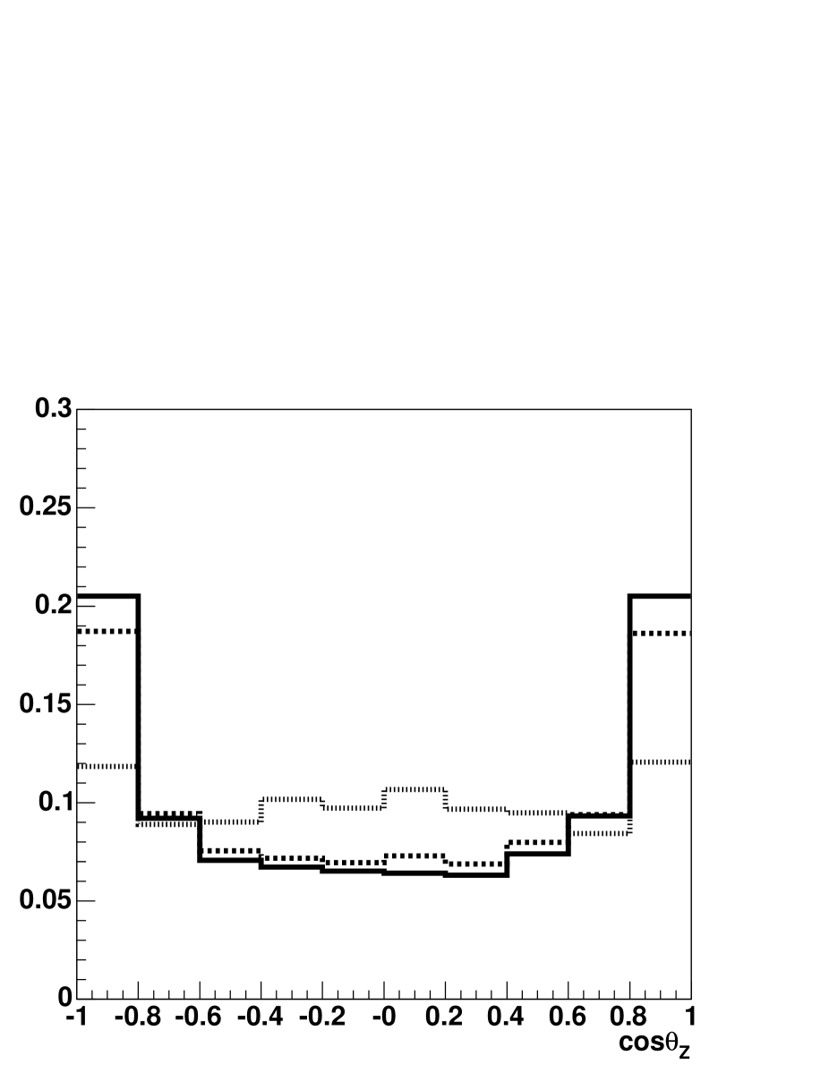
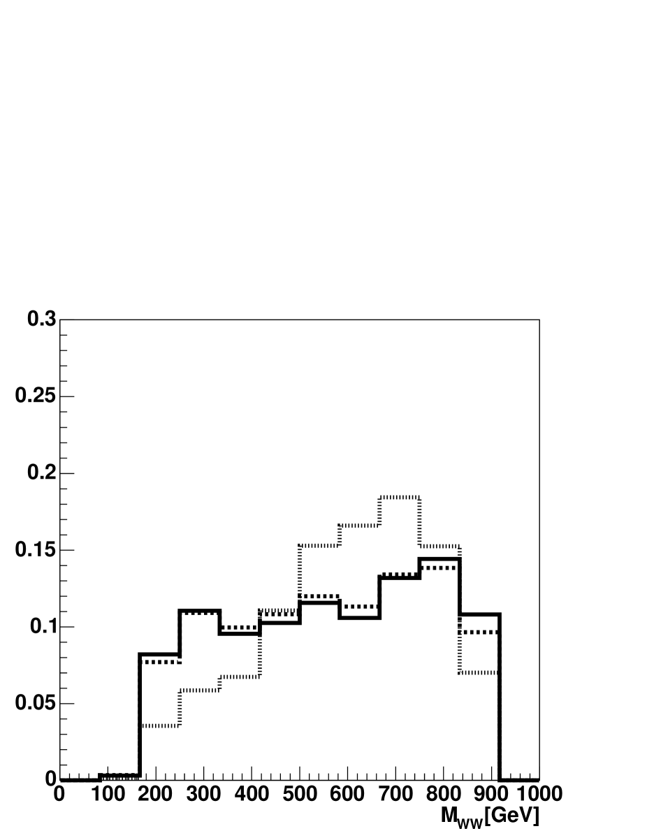
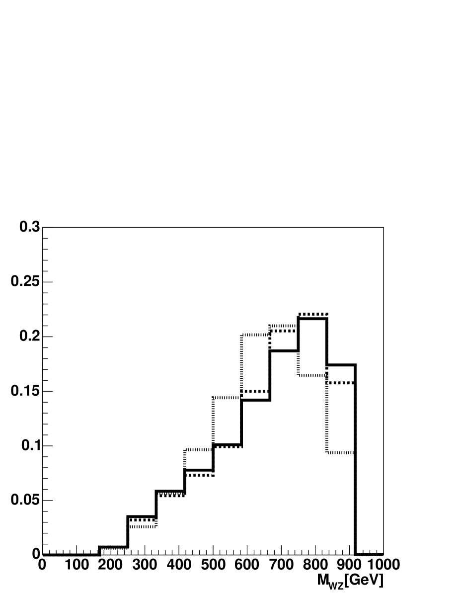
Figure 1: Reconstructed $\cos\theta$, $M_{WW}$, and $M_{WZ}$ signal distributions for $e^{+}e^{-}\rightarrow WWZ$ and both beams polarized. To see the shape dependence the distributions are normalized to the respective total number of events for the Standard Model (solid), $\alpha_{4}=1.6\pi^{2}\approx 15.8$ (dashed) and $\alpha_{5}\approx 15.8$ (dotted).

In triple gauge-boson production processes not all anomalous couplings can be disentangled individually. The process $e^{+}e^{-}\rightarrow W^{+}W^{-}Z$ depends on the $\alpha$ parameters in the two linear combinations $\alpha_{4}+\alpha_{6}$ and $\alpha_{5}+\alpha_{7}$, while the process $e^{+}e^{-}\rightarrow ZZZ$ depends on the single combination $\alpha_{4}+\alpha_{5}+2(\alpha_{6}+\alpha_{7}+\alpha_{10})$. For the study of triple gauge-boson production we concentrate on $\alpha_{4}$ and $\alpha_{5}$ as independent couplings.

In the $WWZ$ final state the rate is dominated by a large SM background that, however, can be substantially reduced using polarized beams that enrich the relative appearance of longitudinal vector-boson polarizations that are sensitive to the EWSB sector. Hence, for $WWZ$ we investigate several running scenarios that are discussed for the ILC: (A) unpolarized, (B) $80\%$ right-handed polarized electrons, and (C) $80\%$ right-handed polarized electrons along with $60\%$ left-handed polarized positrons. For $ZZZ$ the SM background is much smaller and polarization is not substantial.

The total cross section at $\sqrt{s}=1000\;{\rm GeV}$ as calculated with the event generator WHIZARD [42] is given in Table 1. The three-boson final state is characterized by three four-momenta and the bosonic spins. If the bosonic spins are not analyzed, only three kinematical variables are independent, as follows from symmetry considerations and energy-momentum conservation. We choose two invariant masses, $M_{WZ}^{2}=(p_{W}+p_{Z})^{2}$, $M_{WW}^{2}=(p_{W^{+}}+p_{W^{-}})^{2}$, and the angle $\theta$ between the $e^{-}$ beam axis and the direction of the $Z$-boson. The differential cross section $d\sigma(M_{WW},M_{WZ},\cos\theta)$ is discretized into bins denoted by $i,j,k$ for $M_{WZ}$, $M_{WW}$, and $\cos\theta$. Assuming an integrated luminosity of $\int{\cal L}=1000\;{\rm fb}^{-1}$, each bin contains the number of events $N_{ijk}$ given by the differential cross section. We choose 10 bins for $\cos\theta\in[-1,1]$ and 12 bins for $M_{WZ}$ or $M_{WW}\in[0,1000]$ GeV. Since the effective Lagrangian is linear in the anomalous couplings, $N^{\rm theo}_{ijk}(\alpha_{4},\alpha_{5})$ is a polynomial of second order, namely

$$N^{\rm theo}_{ijk}(\alpha_{4},\alpha_{5})=N_{ijk}^{\rm sm}(1+R_{ijk}^{\rm A}\alpha_{4}+R_{ijk}^{\rm B}\alpha_{4}^{2}+R_{ijk}^{\rm C}\alpha_{5}+R_{ijk}^{\rm D}\alpha_{5}^{2}+R_{ijk}^{\rm E}\alpha_{4}\alpha_{5})$$ (79)

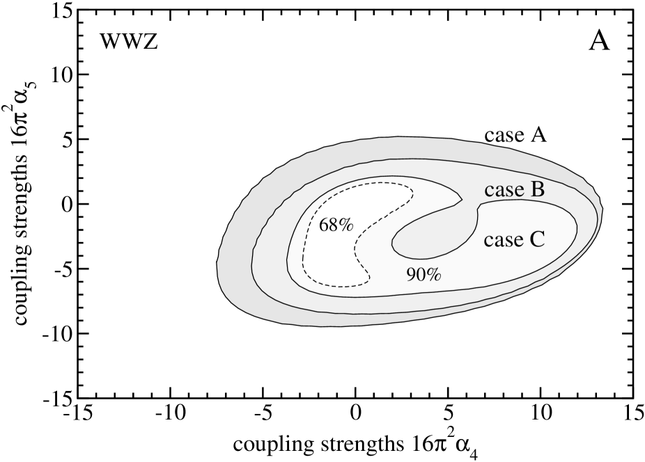
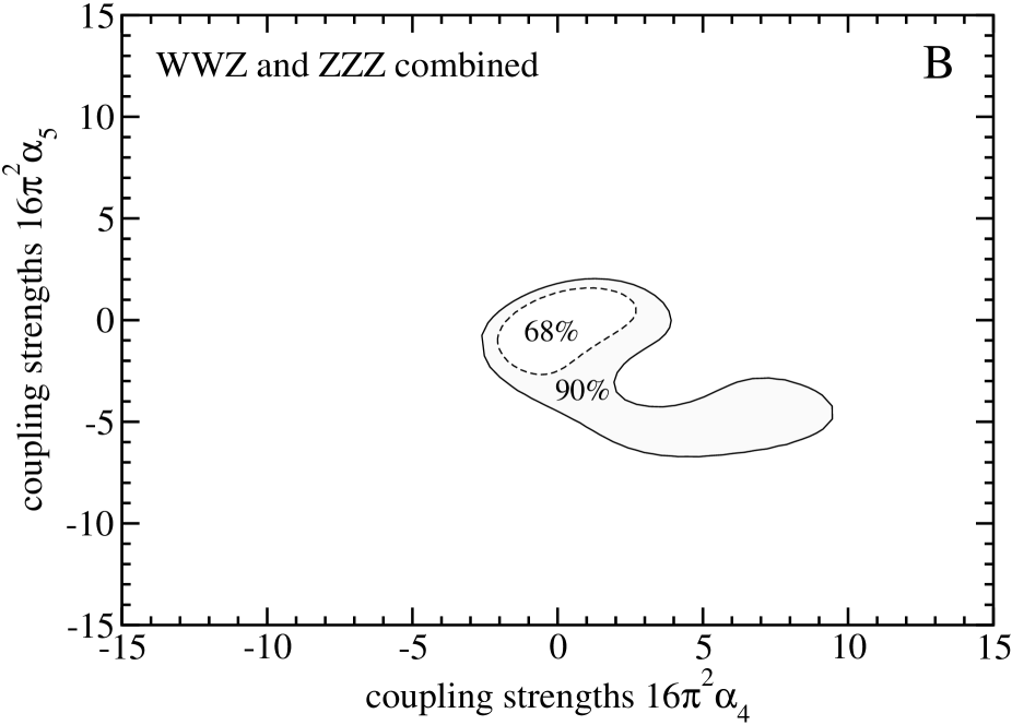
Figure 2: Expected sensitivity for $\alpha_{4}/\alpha_{6}$ and $\alpha_{5}/\alpha_{7}$ at $\sqrt{s}=1000\,{\rm GeV}$. Luminosity assumption 1000 fb^-1. A) $WWZ$-channel only, for an unpolarized beam (A) and the different polarizations cases, $e^{-}$ only polarized (B) and both beams polarized (C) as explained in the text. Solid lines represent $90\%$ confidence level, the dashed line is for 68%, i.e. $\Delta\chi^{2}=2.3$. B) Combined fit using $WWZ$ of case C and $ZZZ$ production. Lines represent $90\%$ (outer line), $68\%$ (inner line) confidence level.

The coefficients $R_{ijk}^{\mathrm{A}\dots\mathrm{E}}$ are determined by reweighting, i.e., for five fixed pairs of anomalous couplings $\alpha_{4}$, $\alpha_{5}$ we recalculate the respective weight, normalized to the weight of the SM event. By inversion, the relative weight $r_{i}$ of each event can then be written as an analytical function of the anomalous couplings,

$$r_{i}=1+a_{i}\alpha_{4}+b_{i}\alpha_{4}^{2}+c_{i}\alpha_{5}+d_{i}\alpha_{5}^{2}+e_{i}\alpha_{4}\alpha_{5}.$$ (80)

The new weights are accumulated for each bin and finally lead to the coefficients in (79). The kinematical variables are reconstructed as will be explained below. Finally we calculate the $\chi^{2}$ contribution given by

$$\chi^{2}=\sum_{i,j,k}\frac{(N^{\rm exp}_{ijk}-N^{\rm theo}_{ijk}(\alpha_{4},\alpha_{5}))^{2}}{\sigma_{ijk}^{2}}\quad,$$ (81)

where $\sigma_{ijk}$ denotes the error, $i,j,k$ are the sums over bins of $M_{WZ}$, $M_{WW}$, and $\cos\theta$. From the miminization of this $\chi^{2}$ distribution we determine $\Delta\alpha_{i}$ (with all $\alpha_{j}=0$). The final result is shown in Fig. 2.

The simulation is done with the WHIZARD event generator [42] using the matrix-element generator O’Mega [43, 44] and the VAMP multi-channel phase space integration package [50]. For the study presented here, we simulate on-shell gauge bosons and decay and hadronize the final state using PYTHIA [45]. Results gained from extending this to full six-fermion matrix elements and spin correlations will be presented in a future publication [46]. The detector is simulated using the fast simulation SIMDET [47].

We produce SM events corresponding to a luminosity of $1000\;{\rm fb}^{-1}$. Three-boson events are reconstructed via six (hadronic) jets utilizing the YCLUS jet-finding algorithm with the Durham recombination scheme. About 32% of all $WWZ$ or $ZZZ$ decays are purely hadronic. Other reconstruction channels are also possible but presently not considered. The dominant background is due to $t\bar{t}\rightarrow b\bar{b}WW\rightarrow 6$ jets. We select events with the kinematical conditions for a combination of missing energy and transverse momentum $E_{\mathrm{mis}}^{2}+p^{2}_{\perp,\mathrm{mis}}<(65\;{\rm GeV})^{2}$ and minimum jet energy $E_{\mathrm{jet}}^{\mathrm{min}}>5\;{\rm GeV}$. Two jets are combined to form a $W$ or a $Z$ requiring

$$\begin{split}-15\;{\rm GeV}&<m^{\mathrm{cand}}-m^{\mathrm{true}}_{W}<\delta M\\ -\delta M&<m^{\mathrm{cand}}-m^{\mathrm{true}}_{Z}<15\;{\rm GeV},\end{split}$$ (82)

where $\delta M=(m^{\mathrm{true}}_{W}+m^{\mathrm{true}}_{Z})/2$, and $m^{\rm true}$ is taken from the Particle Data Group (PDG) [37]. Finally, we take the combination that minimizes the deviation from the PDG values and do a kinematical fit of the bosonic momenta to the total energy and momentum. The top quark is identified via a $b$-jet that is combined with two jets from a $W$ candidate. Top-quark events are vetoed if $|m^{\mathrm{cand}}_{t}-m^{\mathrm{true}}_{t}|<15\;{\rm GeV}$ and the events are consistent with the $t\bar{t}$ topology. The reconstruction efficiency for $WWZ$ is about 12%. This reflects about 36% of all hadronic channels. The purity of the signal is about 98% (case A), 94% (case B), 85% (case C) of $WWZ$. The reconstruction efficiency of $ZZZ$ is about 8%. The purity is 29%, dominated by the large $WWZ$ background. The reconstructed momenta are used to determine the $\chi^{2}$. To minimize fluctuations in the sensitivity, we increase statistics by factors of $5\dots 100$ depending on the process and renormalize $N_{ijk}$ accordingly. The contours and the error intervals are calculated with MINUIT [48].

Table 2: Sensitivity of $\alpha_{4}$ and $\alpha_{5}$ expressed as $1\sigma$ errors. WWZ: two-parameter fit; ZZZ: one-parameter fit; best: best combination of both.

$$\begin{array}[]{c|c||r|r|r||r||r}\hline\cr\lx@intercol\hfil\hfil\lx@intercol\vrule\lx@intercol\vrule\lx@intercol&\lx@intercol\hfil\mbox{WWZ}\hfil\lx@intercol\vrule\lx@intercol\vrule\lx@intercol&\mbox{ZZZ}&\mbox{best}\\ \lx@intercol\hfil\hfil\lx@intercol\vrule\lx@intercol\vrule\lx@intercol&\mbox{no pol.}&e^{-}\mbox{ pol.}&\mbox{both pol.}&\mbox{no pol.}\\ \hline\cr 16\pi^{2}\Delta\alpha_{4}&\sigma^{+}&9.79&4.21&1.90&3.94&1.78\\ &\sigma^{-}&-4.40&-3.34&-1.71&-3.53&-1.48\\ \hline\cr 16\pi^{2}\Delta\alpha_{5}&\sigma^{+}&3.05&2.69&1.17&3.94&1.14\\ &\sigma^{-}&-7.10&-6.40&-2.19&-3.53&-1.64\\ \hline\cr\end{array}$$

Results are shown in Fig. 2 and Tab. 2. For $WWZ$ we give in Fig. 2A the 90% contours for the different polarization cases A, B, and C, and for both beams polarized also the 68% contour. The respective $\Delta\alpha_{i}$ are given in Tab. 2. Note that for $WWZ$ two parameters are independent, while for $ZZZ$ only one. Hence for $WWZ$ we get $\Delta\alpha_{4}=\Delta\alpha_{6}$, $\Delta\alpha_{5}=\Delta\alpha_{7}$, and no sensitivity to $\alpha_{10}$. For $ZZZ$ we have $\Delta\alpha_{4}=\Delta\alpha_{5}=\frac{1}{2}\Delta\alpha_{6}=\frac{1}{2}\Delta\alpha_{7}=\frac{1}{2}\Delta\alpha_{10}$. We find that the sensitivity strongly increases with polarization, cf. the different cases A, B, and C. A best combined fit for triple boson production is given in Fig. 2B.

The sensitivity could be further improved by using the information provided by the angular distribution of jets, since the EWSB sector mainly affects the longitudinal polarization directions of vector bosons. This will be covered in a future publication [46].

6 Vector-Boson Scattering Processes at the ILC

In this section we consider those six-fermion processes in $e^{+}e^{-}$ and $e^{-}e^{-}$ collisions that depend on quartic gauge couplings via quasi-elastic weak-boson scattering subprocesses, i.e., $VV\to VV$, where $V=W^{\pm},Z$. We use full six-fermion matrix elements and thus do not rely on simplifications such as the effective $W$ approximation, the Goldstone-boson equivalence theorem, or the narrow-width approximation for vector bosons.

For the simulation we assume a c.m. energy of $1\;{\rm TeV}$ and a total luminosity of $1000\;{\rm fb}^{-1}$ in the $e^{+}e^{-}$ mode. Beam polarization of 80% for electrons and 40% for positrons is also assumed. Since the six-fermion processes under consideration contain contributions from the triple weak-boson production processes considered in the previous section ($ZZ$ or $W^{+}W^{-}$ with neutrinos of second and third generation as well as a part of $\nu_{e}\bar{\nu}_{e}WW(ZZ)$, $e\nu_{e}WZ$ and $e^{+}e^{-}W^{+}W^{-}$ final states), there is no distinct separation of signal and background. Signal processes in a separate analysis are thus affected by all other signal processes as well as by pure background.

The present study extends the previous study [49] which considered a restricted set of channels and parameters. In addition to the backgrounds considered there, we include single weak-boson production in the background simulation for completeness. We take initial-state radiation into account when generating events. For the generation of $t\bar{t}$ events we use PYTHIA [45]. The event samples are generated by the multi-purpose event generator O’Mega/WHIZARD [43, 42, 44], using exact six-fermion tree-level matrix elements. No flavor summation is necessary since all possible quark final states are generated. Hadronization is done with PYTHIA. We use the SIMDET [47] program to produce the detector response of a possible ILC detector.

Table 3 contains a summary of all generated processes used for analysis and their corresponding cross sections. For pure background processes a full $1\;{\rm ab}^{-1}$ sample is generated. All signal processes are generated with higher statistics. Single weak-boson processes and $q{\bar{q}}$ events are generated with an additional cut on $M(q{\bar{q}})>130\;{\rm GeV}$ to reduce the number of generated events.

Process	Subprocess	$\sigma\;[{\rm fb}]\quad$
$e^{+}e^{-}\to\nu_{e}\bar{\nu}_{e}q\bar{q}q\bar{q}$	$W^{+}W^{-}\to W^{+}W^{-}$	23.19
$e^{+}e^{-}\to\nu_{e}\bar{\nu}_{e}q\bar{q}q\bar{q}$	$W^{+}W^{-}\to ZZ$	7.624
$e^{+}e^{-}\to\nu\bar{\nu}q\bar{q}q\bar{q}$	$V\to VVV$	9.344
$e^{+}e^{-}\to\nu eq\bar{q}q\bar{q}$	$WZ\to WZ$	132.3
$e^{+}e^{-}\to e^{+}e^{-}q\bar{q}q\bar{q}$	$ZZ\to ZZ$	2.09
$e^{+}e^{-}\to e^{+}e^{-}q\bar{q}q\bar{q}$	$ZZ\to W^{+}W^{-}$	414.000
$e^{+}e^{-}\to b\bar{b}X$	$e^{+}e^{-}\to t\bar{t}$	331.768
$e^{+}e^{-}\to q\bar{q}q\bar{q}$	$e^{+}e^{-}\to W^{+}W^{-}$	3560.108
$e^{+}e^{-}\to q\bar{q}q\bar{q}$	$e^{+}e^{-}\to ZZ$	173.221
$e^{+}e^{-}\to e\nu q\bar{q}$	$e^{+}e^{-}\to e\nu W$	279.588
$e^{+}e^{-}\to e^{+}e^{-}q\bar{q}$	$e^{+}e^{-}\to e^{+}e^{-}Z$	134.935
$e^{+}e^{-}\to X$	$e^{+}e^{-}\to q\bar{q}$	1637.405

Table 3: Generated processes and cross sections for signal and background for $\sqrt{s}=1\;{\rm TeV}$, polarization 80% left for electron and 40% right for positron beam. For each process, those final-state flavor combinations are included that correspond to the indicated signal or background subprocess.

The observables sensitive to the quartic couplings are the total cross section (either reduction or increase depending on the interference term in the amplitude and the point in parameter space), and modification of the differential distributions in vector-boson production angle and decay angle. This is not a full set of observables, but some sensitive event variables, for example transverse momentum, cannot be used since the contribution of longitudinally polarized weak bosons is dropping faster than for transversally polarized weak bosons with increasing transverse momentum, and a transverse-momentum cut is unavoidable to suppress the background in the analysis.

The event selection is done by a cut-based approach similar to the previous analysis [49]. The general steps in the analysis are the use of the final state $e^{-}$($e^{+}$) to tag background (signal in $e{\nu}_{e}WZ$ case), a cut on transverse momentum, and

${e^{+}}{e^{-}}\rightarrow$	${e^{-}}{e^{-}}\rightarrow$	${\alpha}_{4}$	${\alpha}_{5}$	${\alpha}_{6}$	${\alpha}_{7}$	${\alpha}_{10}$
${W^{+}}{W^{-}}\rightarrow{W^{+}}{W^{-}}$	${W^{-}}{W^{-}}\rightarrow{W^{-}}{W^{-}}$	+	+	-	-	-
${W^{+}}{W^{-}}\rightarrow ZZ$		+	+	+	+	-
${W^{\pm}}Z\rightarrow{W^{\pm}}Z$	${W^{-}}Z\rightarrow{W^{-}}Z$	+	+	+	+	-
$ZZ\rightarrow ZZ$	$ZZ\rightarrow ZZ$	+	+	+	+	+

Table 4: Sensitivity to quartic anomalous couplings for all quasi-elastic weak-boson scattering processes accessible at the ILC. In addition to the $e^{+}e^{-}$ processes considered in this paper, we list the $e^{-}e^{-}$ processes for illustration.

missing mass and energy. Realistic ZVTOP b-tagging [51] is used whenever possible to improve the signal-to-background separation. Finally, we apply cuts around the nominal masses of weak bosons to accept only well-reconstructed events.

The extraction of quartic gauge couplings from reconstructed kinematic variables is done by a binned likelihood fit. For each signal process, we generate statistics much larger than the nominal $1000\;{\rm fb}^{-1}$ for $e^{+}e^{-}$ and pass the events through the detector simulation. Each event is described by reconstructing four kinematic variables: the event mass, the absolute value of production angle cosine, and the absolute values of decay angle cosines for each reconstructed weak boson. Only absolute value of the production and decay angles are used since there is no possibility to resolve quark-antiquark and $W^{+}W^{-}$ ambiguities.

Starting from an unweighted event sample as generated by WHIZARD, we use the complete matrix elements encoded in the event generator itself to reweight each event as a function of the quartic gauge couplings. Each Monte-Carlo event is weighted by

$$R({\alpha}_{i},{\alpha}_{j})=1+A{{\alpha}_{i}}+B{{\alpha}_{i}}^{2}+C{{\alpha}_{j}}+D{{\alpha}_{j}}^{2}+E{{\alpha}_{i}}{{\alpha}_{j}}.$$ (83)

The function $R({\alpha}_{i},{\alpha}_{j})$ describes the quadratic dependence of the differential cross section on the anomalous couplings. It is obtained in the following way: using the generated SM events (i.e., ${\alpha}_{i}\equiv 0$), we recalculate the matrix element for each event at five different points in $\alpha_{i},\alpha_{j}$ space and solve a set of linear equations for $A$,$B$,$C$,$D$ and $E$. Due to the linear functional dependence of the amplitude [52] on the couplings, five points are enough to determine the coefficients for the weighting function. The choice of the points varies from process to process in order to fulfil the following conditions: the distance of the point(s) from the SM value should be large enough not to come into numerical instabilities when solving the equations, and at the same time small enough not to come into the region were phase space population would be significantly different from the SM.

The obtained four-dimensional event distributions are fitted with MINUIT [48], maximizing the likelihood as a function of ${\alpha}_{i}$,${\alpha}_{j}$ by taking the SM Monte-Carlo sample as “data”:

$$L(\alpha_{p},\alpha_{q})=-\sum\limits_{i,j,k,l}{N^{SM}}(i,j,k,l)\ln\left({N^{{\alpha}_{p},{\alpha}_{q}}{}}(i,j,k,l)\right)+\sum\limits_{i,j,k,l}{N^{{\alpha}_{p},{\alpha}_{q}}}(i,j,k,l)$$ (84)

where $i$ runs over the reconstructed event energy, $j$ over the production angle, $k$ and $l$ over the decay angles. ${N^{SM}}(i,j,k,l)$ are the “data” which correspond to the SM Monte Carlo sample, and ${N^{{\alpha}_{p},{\alpha}_{q}}}(i,j,k,l)$ is the sum of the same SM events in this bin, each reweighted by $R({\alpha}_{p},{\alpha}_{q})$. Pure background events have $R({\alpha}_{p},{\alpha}_{q})=1$, and for background coming from other sensitive processes the proper weight is taken into account. After a separate analysis for each process (see Table 4), we perform a combined fit. A small fraction of doubly-counted events that remains after the single process analysis is uniquely assigned to one or another set according to the distance from the nominal mass of the weak boson pair (for example $WW$ or $ZZ$).

7 Combined Results and Resonance Interpretation

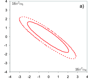
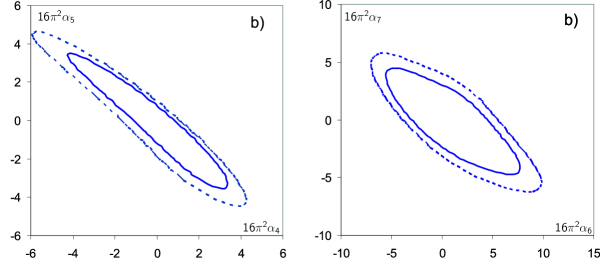
Figure 3: Expected sensitivity (combined fit for all sensitive processes) to quartic anomalous couplings for a 1000 fb^-1 $e^{+}e^{-}$ sample. The full line (inner one) represents 68%, the dotted (outer) one 90% confidence level. a) conserved $SU(2)_{c}$ case b) broken $SU(2)_{c}$ case.

coupling	$\sigma-$	$\sigma+$
$\alpha_{4}$	-1.41	1.38
$\alpha_{5}$	-1.16	1.09

Table 5: The expected sensitivity from 1000 fb${}^{-1}e^{+}e^{-}$ sample at 1 TeV in the $SU(2)_{c}$ conserving case, positive and negative one sigma errors given separately.

coupling	$\sigma-$	$\sigma+$
$\alpha_{4}$	-2.72	2.37
$\alpha_{5}$	-2.46	2.35
$\alpha_{6}$	-3.93	5.53
$\alpha_{7}$	-3.22	3.31
$\alpha_{10}$	-5.55	4.55

Table 6: The expected sensitivity from 1000 fb${}^{-1}e^{+}e^{-}$ sample at 1 TeV in the broken $SU(2)_{c}$ case, positive and negative 1 sigma errors given separately.

In Table 6 and Table 6 we combine our results for the measurement of anomalous electroweak couplings for an integrated luminosity of $1000\;{\rm fb}^{-1}$ in the ${e^{+}}{e^{-}}$ mode, assuming $SU(2)_{c}$ conservation and non-conservation, respectively. In Fig. 3, the results are displayed in graphical form, projecting the multi-dimensional exclusion region in $\alpha$ space around the reference point $\alpha_{i}\equiv 0$ onto the two-dimensional subspaces $(\alpha_{4},\alpha_{5})$ and $(\alpha_{6},\alpha_{7})$

In order to get a more intuitive physical interpretation in terms of a new-physics scale, in this section we transform anomalous couplings into resonance parameters, as described in Sec. 3. To this end, we also include the expected ILC results for triple gauge couplings and oblique corrections in the fit. Assuming one particular resonance at a time, for each measured value of some $\alpha$ parameter, we may deduce the properties of the resonance that would result in this particular value. Inserting the values that correspond to the sensitivity bound obtained by the experimental analysis, we get a clear picture on the possible sensitivity to resonance-like new physics in the high-energy region.

7.1 $J=0$ Channel

7.1.1 Scalar Singlet: $\sigma$

(i) We first consider the isospin conserving case, $h_{\sigma}=0$, which leads to $\alpha_{7}=\alpha_{10}=0$. Since $\alpha_{4}=\alpha_{6}=0$, there is only a dependence on ${\alpha}_{5}$ as a free parameter. After the fit, we get $\sigma_{\alpha_{5}}=0.42$ for the symmetric error or $-0.452<{\alpha}_{5}<0.397$ for the asymmetric ones at $1\sigma$ level.

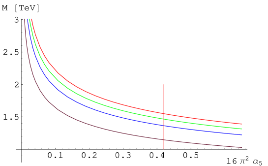
Figure 4: Mass of the scalar singlet resonance in the isospin-conserving case as a function of ${\alpha}_{5}$, with the resonance’s width to mass ratio $f_{\sigma}$ equal to $1.0$ in red, $0.8$ in green, $0.6$ in blue, and $0.3$ in brown, respectively. The vertical line in the plot is the $1\,\sigma$ limit on ${\alpha}_{5}$.

Expressing the width of the resonance as a fraction of its width, $\Gamma_{\sigma}=f_{\sigma}M_{\sigma}$, it is possible to solve Equ. (19) and $\alpha_{5}=g_{\sigma}^{2}\frac{v^{2}}{8M_{\sigma}^{2}}$ to obtain the resonance mass as a function of the quartic coupling and this fraction:

$$M_{\sigma}=v\left(\frac{4\pi f_{\sigma}}{3\alpha_{5}}\right)^{\frac{1}{4}}$$ (85)

In Fig. 4, we plot the mass of a scalar singlet resonance as a function of the coupling for a given width. The vertical line in the plot is the $1\sigma$ error for a calculation of the mass from a given value of the width.

$f_{\sigma}=\frac{\Gamma_{\sigma}}{M_{\sigma}}$	$1.0$	$0.8$	$0.6$	$0.3$
$M_{\sigma}\,[{\rm TeV}]$	$1.55$	$1.46$	$1.36$	$1.15$

Table 7: Mass reach for the scalar resonance in the SU(2)_c conserving case depending on different resonance widths.

(ii) If we allow for isospin violation, $\alpha_{4}$ and $\alpha_{6}$ are still zero, leaving the three free parameters $\alpha_{5}$, $\alpha_{7}$ and $\alpha_{10}$ for the fit. With only two independent variables, the system of equations (18a), (19) is overconstrained with the additional relation

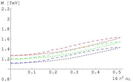
Figure 5: Scalar singlet with isospin breaking: On the left, $1\,\sigma$ contour in the ${\alpha}_{5}-{\alpha}_{7}$ plane. On the right, the dependence of the resonance mass on ${\alpha}_{5}$ along the contour for $f_{\sigma}=1$ (width equal to the mass) in red, $f_{\sigma}=0.8$ in green, and $f_{\sigma}=0.6$ in blue. The dashed and wide-dashed lines correspond to the different branches of the solution of ${\alpha}_{7}=\mathcal{F}[\alpha_{5}]$, respectively.

$$\alpha_{7}^{2}=2\alpha_{5}\alpha_{10}.$$ (86)

By this equation one is able to eliminate one of the couplings from further consideration. We will choose to eliminate $\alpha_{10}$. Solving the system of equations, it is now possible to express the mass as a function of the width, $\alpha_{5}$ and $\alpha_{7}$:

$$M_{\sigma}=v\left(\frac{4\pi\alpha_{5}f_{\sigma}}{2\alpha_{5}^{2}+(\alpha_{5}+\alpha_{7})^{2}}\right)^{\frac{1}{4}}.$$ (87)

if we limit ourselves to the case that we vary the couplings only

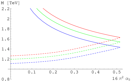
Figure 6: Allowed region for a scalar singlet resonance with isospin breaking as a function of ${\alpha}_{5}$ between the upper (full) and lower bound (dashed). Ratio of width to mass of the resonance equal to $1.0$ (red), $0.8$ (green), and $0.6$ (blue), respectively.

along the $1\sigma$ contour in the $\alpha_{5}$,$\alpha_{7}$ plane, we end up with the result shown in Fig. 5.

$f_{\sigma}=\frac{\Gamma_{\sigma}}{M_{\sigma}}$	$1.0$	$0.8$	$0.6$
$M_{\sigma}\,[{\rm TeV}]$	$1.39$	$1.32$	$1.23$

Table 8: Mass reach for the scalar singlet resonance in the case of isospin breaking depending on the width to mass ratio $f_{\sigma}$. We use an average mass along the contour.

The lower of the two dashed curves gives a lower limit on the allowed region. On the other hand, one can look for the maximum mass for the $\alpha$ parameters within the $1\sigma$-contour. This is equivalent to minimizing the width (19) by $g_{\sigma}=-2h_{\sigma}$, which yields a maximum mass (depending on the allowed $\alpha$ parameters) for $\alpha_{5}=-\alpha_{7}$ of

$$M_{\sigma}=v\left(\frac{2\pi f_{\sigma}}{\alpha_{5}}\right)^{\frac{1}{4}}.$$ (88)

Fig. 6 shows the allowed region for different values of the width to mass ratio of the scalar singlet resonance. This means that a scalar singlet resonance corresponding to measured $\alpha_{5,7}$ values lying in the simulated $1\,\sigma$ contour cannot be heavier than the given upper limit.

7.1.2 Scalar Triplet: $\pi$

(i) In principle, for a scalar triplet, there is no isospin-conserving limit, since $SU(2)$ breaking is necessary to couple a triplet to two identical bosonic triplets. Nevertheless, there is a case, where $h_{\pi}=k_{\pi}=0$ and only $h^{\prime}_{\pi}\neq 0$. In that case, the SM fields couple in an $SU(2)$ invariant way, and the isospin breaking resides in the coupling of the new resonances only. Therefore, a resonance with such a coupling would – to the order we are considering – leave no trace in the isospin-breaking operators, but only gives a contribution to $\mathcal{L}_{5}$. So experimentally, the isospin breaking is not detectable without direct access to the heavy resonances. Hence, again at leading order, there is no contribution to the width of the $\pi^{\pm}$ from electroweak gauge bosons. In this case, we regain the formula for the singlet case,

$$M_{\pi^{0}}=v\left(\frac{4\pi f_{\pi^{0}}}{3\alpha_{5}}\right)^{\frac{1}{4}},$$ (89)

while the charged resonance is not accessible in gauge boson scattering. Such a case would experimentally be indistinguishable from a singlet scalar. The bounds from the isospin-conserving singlet case also apply here.

(ii) If we allow for general isospin-breaking couplings, from Equ. (25a) we get the constraint

$$\alpha_{7}^{2}=2\alpha_{5}(\alpha_{6}+\alpha_{10}),$$ (90)

which is the generalization of the singlet case. The correspondence between the singlet and the triplet discussed above goes even further. If we put $h_{\pi}$ to zero, the formula for the $\alpha$s as well as for the width between singlet and triplet correspond to each other with the identification: $g_{\sigma}\leftrightarrow h^{\prime}_{\pi}$, $h_{\sigma}\leftrightarrow k_{\pi}$. In that case, $\alpha_{6}$ is zero, the charged resonance decouples at leading order, the two relations (86) and (90) are then identical, as are the formula for the mass of the neutral resonance as a function of $\alpha_{5,7}$. So for the case $h_{\pi}=0$ we can reuse the results from the fit for the isospin-breaking singlet.

Allowing finally also for nonvanishing $h_{\pi}$ (i.e. nonvanishing $\alpha_{6}$), we again use the overconstraining to eliminate $\alpha_{10}$. Solving the remaining system we get:

$$M_{\pi^{\pm}} =\;v\left(\frac{4\pi f_{\pi^{\pm}}}{\alpha_{6}}\right)^{\frac{1}{4}}$$ (91a)

$$M_{\pi^{0}} =\;v\left(\frac{4\pi\alpha_{5}f_{\pi^{0}}}{2\alpha_{5}^{2}+(\alpha_{5}+\alpha_{7})^{2}}\right)^{\frac{1}{4}}$$ (91b)

The formula for the neutral component still is the same as for the nonconserving singlet case, which can be understood by using the

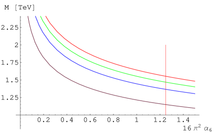
Figure 7: Dependence of the resonance mass for the charged scalar triplet component on ${\alpha}_{6}$ for different assumed width to mass ratios ($f_{\pi}=\Gamma_{\pi}/M_{\pi}=1.0$ in red, $0.8$ in blue, $0.3$ in brown, respectively). The red vertical line represents the maximal value of ${\alpha}_{6}$ along the $1\,\sigma$ surface.

above correspondence and the replacing $2k_{\pi}\to 2k_{\pi}+h_{\pi}$ in the formulas for the $\alpha$s and the width. So the limits for the neutral component remain the same, and figures 5 and 6 are also applicable here. The mass reach for the scalar triplet in the isospin breaking case is given in table 9.

$f_{\pi}=\frac{\Gamma_{\pi}}{M_{\pi}}$	$1.0$	$0.8$	$0.6$	$0.3$
$M_{\pi^{0}}\,[{\rm TeV}]$	$1.39$	$1.32$	$1.23$	—
$M_{\pi^{\pm}}\,[{\rm TeV}]$	$1.55$	$1.47$	$1.37$	$1.15$

Table 9: Dependence of the mass reach for scalar triplet resonances on different resonance widths. For the neutral narrow state the mass reach is already below $1\,{\rm TeV}$.

A technical remark: $\alpha_{5}$ and $\alpha_{6}$ must be positive in order to get real solutions for the mass. The solutions for the mass decouple ${\alpha}_{6}$ and ${\alpha}_{5},{\alpha}_{7}$ from each other, but we can still use the error matrix and the relation $\mathcal{F}({\alpha}_{5},{\alpha}_{6},{\alpha}_{7})=1$ to fix the points on the $1\,\sigma$ surface.

7.1.3 Scalar Quintet: $\phi$

(i) For isospin conservation, only $g_{\phi}$ and hence only $\alpha_{4}$ is non-vanishing. Solving the system (31a), (32a) yields

$$M_{\phi}=v\left(\frac{4\pi f_{\phi}}{\alpha_{4}}\right)^{\frac{1}{4}}$$ (92)

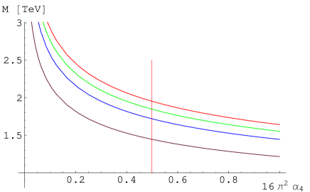
Figure 8: Dependence of the resonance mass for the scalar quintet on the $\alpha$ parameters for different width to mass ratios, $f_{\phi}=\Gamma_{\phi}/M_{\phi}=1.0$ (red), $0.8$ (blue), $0.6$ (green), and $0.3$ (brown), respectively. On the left: Isospin-conserving case, degenerate mass of the whole multiplet as a function of $\alpha_{4}$. On the right: Special isospin-breaking case with only $h_{\phi}^{\prime}$ different from zero. Mass of the neutral component as a function of $\alpha_{5}$. The vertical red line represents the $1\,\sigma$ limit for $\alpha_{4}$ and $\alpha_{5}$, respectively.

$f_{\phi}=\frac{\Gamma_{\phi}}{M_{\phi}}$	$1.0$	$0.8$	$0.6$	$0.3$
$M_{\phi}\,[{\rm TeV}]$	$1.95$	$1.85$	$1.72$	$1.45$

$f_{\phi^{0}}=\frac{\Gamma_{\phi^{0}}}{M_{\phi^{0}}}$	$1.0$	$0.8$	$0.6$	$0.3$
$M_{\phi^{0}}\,[{\rm TeV}]$	$2.06$	$1.96$	$1.82$	$1.53$

Table 10: Mass reach for the scalar quintet depending on different ratios of width to mass. On the left, the $SU(2)_{c}$ conserving case, on the right the special isospin-breaking case with only $h^{\prime}_{\phi}\neq 0$.

The results for the isospin-conserving case are shown on the left of Fig. 8 and Table 10.

(ii) For the case of broken isospin symmetry, we first consider the case that only $h^{\prime}_{\phi}\neq 0$, so that only $\alpha_{5}$ is nonvanishing. The charged and doubly-charged resonances do not get a contribution to their width at leading order, while solving for the mass of the neutral state results in

$$M_{\phi^{0}}=v\left(\frac{2\pi f_{\phi^{0}}}{\alpha_{5}}\right)^{\frac{1}{4}}.$$ (93)

The fit and the $1\,\sigma$ reach are shown in the right plot of Fig. 8 and Table 10 also on the right.

There is a further special case when $\alpha_{4}=-\alpha_{6}$, in which the charged resonance does not get a contribution to the width. Here also a singularity for the neutral state appears where the denominator for the mass of the neutral state vanishes. We ignore this case here.

The next step is that we allow for nonzero $g_{\phi}$ and $h^{\prime}_{\phi}$, which results in non-zero $\alpha_{4},\alpha_{5}$ and

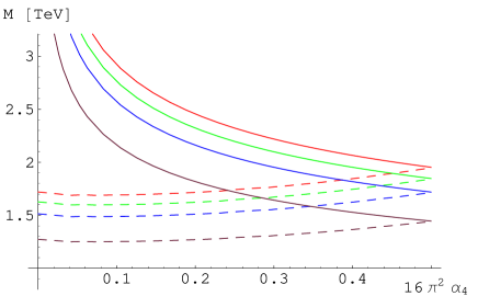
Figure 9: Dependence of the mass of the neutral component of a scalar quintet resonance for the case with only $g_{\phi},h^{\prime}_{\phi}$ non-zero, as a function of $\alpha_{4}$ for different width to mass ratios: in red $f_{\phi}=\Gamma_{\phi}/M_{\phi}=1.0$, in green $0.8$, in blue $0.6$, and in brown $0.3$. The red vertical line represents the maximal value of $\alpha_{4}$.

$f_{\phi}=\frac{\Gamma_{\phi}}{M_{\phi}}$	$1.0$	$0.8$	$0.6$	$0.3$
$M_{\phi 0}\,[{\rm TeV}]$	$1.77$	$1.67$	$1.55$	$1.31$

Table 11: Mass reach for the neutral component of the scalar quintet in the case with only $g_{\phi},h^{\prime}_{\phi}$ non-zero, depending on different width to mass ratios.

$\alpha_{7}$ with the constraint $\alpha^{2}_{7}=\alpha_{5}\alpha_{4}$. Note that the term proportional to $gh^{\prime}$ in the width of the neutral state cancels out – and hence the dependence on $\alpha_{7}$. In this special case, the formula for the masses of the charged and doubly-charged states remains the same as Equ. (92). The mass reach equals the isospin-conserving case. In principle, isospin non-conservation can be detected by the different width of the neutral state. The solution for that component becomes

$$M_{\phi^{0}}=v\left(\frac{4\pi f_{\phi^{0}}}{\alpha_{4}+2\alpha_{5}}\right)^{\frac{1}{4}},$$ (94)

with constraints ${\alpha}_{4}>0$ and ${\alpha}_{5}>0$.

For the completely general case of isospin breaking, the relation between the couplings is now a generalization of the triplet case, namely

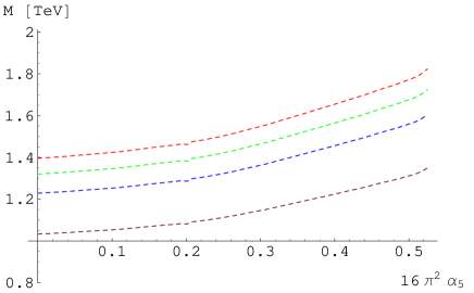
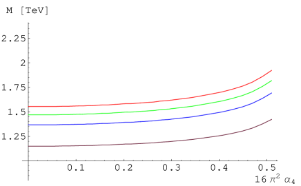
Figure 10: Dependence of the mass of the neutral (left) and the charged component (right) of a scalar quintet resonance in the completely general case, as a function of $\alpha_{4}$ for different width to mass ratios: in red $f_{\phi}=\Gamma_{\phi}/M_{\phi}=1.0$, in green $0.8$, in blue $0.6$, and in brown $0.3$. The red vertical line represents the maximal value of $\alpha_{4}$. The doubly-charged component remains the same as in the isospin-conserving case, shown on the left of Fig. 8.

$f_{\phi}=\frac{\Gamma_{\phi}}{M_{\phi}}$	$1.0$	$0.8$	$0.6$	$0.3$
$M_{\phi\pm\pm}\,[{\rm TeV}]$	$1.95$	$1.85$	$1.72$	$1.45$
$M_{\phi\pm}\,[{\rm TeV}]$	$1.64$	$1.55$	$1.44$	$1.21$
$M_{\phi 0}\,[{\rm TeV}]$	$1.55$	$1.46$	$1.35$	$1.14$

Table 12: Mass reach for the scalar quintet in most general case.$M_{\phi 0}$ and $M_{\phi\pm}$ are averages over the lower limit curves.

$$\alpha_{7}^{2}=2\alpha_{5}\left(\frac{1}{2}\alpha_{4}+\alpha_{6}+\alpha_{10}\right),$$ (95)

to again eliminate $\alpha_{10}$.

We obtain the solution for the masses

$$M_{\phi^{\pm\pm}} =\;v\left(\frac{4\pi f_{\phi^{\pm\pm}}}{\alpha_{4}}\right)^{\frac{1}{4}}$$ (96a)

$$M_{\phi^{\pm}} =\;v\left(\frac{4\pi f_{\phi^{\pm}}}{\alpha_{4}+\alpha_{6}}\right)^{\frac{1}{4}}$$ (96b)

$$M_{\phi^{0}} =\;v\left(\frac{12\pi\alpha_{5}f_{\phi^{0}}}{(\sqrt{\alpha_{4}\alpha_{5}}-2\alpha_{5})^{2}+2(\alpha_{7}+\alpha_{5})^{2}}\right)^{\frac{1}{4}}$$

$$\;=v\left(\frac{12\pi f_{\phi^{0}}}{(\sqrt{\alpha_{4}}-2\sqrt{\alpha_{5}})^{2}+2(\sqrt{\alpha_{4}+2\alpha_{6}+2\alpha_{10}}+\sqrt{\alpha_{5}})^{2}}\right)^{\frac{1}{4}}$$ (96c)

For the neutral state, the first formula is in correspondence to those for the non-isospin conserving singlet and triplet case, while the second one is better suited for taking the limit to the isospin-conserving case.

7.2 $J=1$ Channel

7.2.1 Vector Singlet: $\omega$

(ii) For the vector singlet, isospin breaking has to be involved. Concerning the analysis and the fit, we ignore the parameter $k_{\omega}$ because it has no physical meaning in terms of the resonance mass and width, at least in the order we are considering. So all eight nonvanishing $\alpha$ parameters are the same,

$$\alpha_{1}=\alpha_{2}=\alpha_{4}=\alpha_{7}=-\alpha_{5}=-\alpha_{6}=-\alpha_{8}=-\alpha_{9}$$ (97)

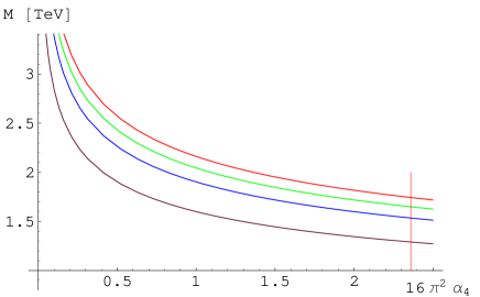
Figure 11: Dependence of the mass of a singlet vector resonance on ${\alpha}_{4}$ for different assumed $f_{\pi}=\Gamma_{\pi}/M_{\pi}=1.0$ in red, $0.8$ in blue, $0.3$ in brown, respectively. The condition $\ell_{\omega}=0$ is used.

$f_{\omega}=\frac{\Gamma_{\omega}}{M_{\omega}}$	$1.0$	$0.8$	$0.6$	$0.3$
$M_{\omega}\,[{\rm TeV}]$	$1.74$	$1.65$	$1.53$	$1.29$

Table 13: Mass reach for a singlet vector resonance in the case $\ell_{\omega}=0$ for different assumed width to mass ratios: $f_{\omega}=\Gamma_{\omega}/M_{\omega}=1.0$ (red), $0.8$ (blue), $0.6$ (green), and $0.3$ (brown), respectively

Furthermore, the three non-zero $\alpha^{\lambda}$ parameters are also the same, $\alpha_{2}^{\lambda}=\alpha_{5}^{\lambda}=-\alpha_{1}^{\lambda}$. Including the parameter $k_{\omega}$ which could, of course, occur in the $\alpha$ parameters, changes the above result to

$$\alpha_{1}=\alpha_{2}=\alpha_{4} =\alpha_{7}=-\alpha_{5}=-\alpha_{6}=-\alpha_{8}$$

$$\alpha_{9} =-(\alpha_{3}+\alpha_{4})\quad.$$

Using only the parameters $\alpha_{4}$ and $\alpha_{2}^{\lambda}$ eliminates the dependence on $k_{\omega}$. The mass of the singlet resonance is then given by

$$M_{\omega}=v\left(\frac{12\pi\alpha_{4}f_{\omega}}{\alpha^{2}_{4}+\frac{1}{2}(\alpha_{2}^{\lambda})^{2}}\right)^{\frac{1}{4}}.$$ (98)

For the fit we used the simplifying assumption $\ell_{\omega}=0$,

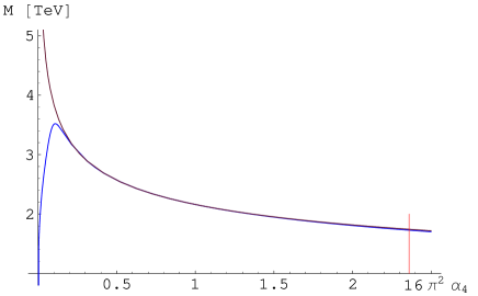
Figure 12: Dependence of the mass of a singlet vector resonance on ${\alpha}_{4}$ including the parameter $\ell_{\omega}$ for different assumed width to mass ratios: on the left 1.0, and 0.3 on the right. The red curve is the $1\,\sigma$ upper limit for $\alpha_{4}$. The allowed resonance mass is between the blue and the brown curve, which are for the maximally and minimally allowed values of $\lambda_{Z}$ in [41], respectively.

which yields the simplified mass formula

$$M_{\omega}=v\left(\frac{12\pi f_{\omega}}{\alpha_{4}}\right)^{\frac{1}{4}}.$$ (99)

So this reduces to a one-parameter fit. As a cross-check, the error matrix for $\Delta g^{Z}_{1},\Delta\kappa^{Z},\lambda^{Z}$ from [41] has been reproduced. The limits for the vector singlet in the case of vanishing $\ell_{\omega}$ are given in Fig. 11 and Table 13.

Taking also $\ell_{\omega}$ into account, one can solve for the mass of the vector resonance as a function of $\alpha_{4}$, $f_{\omega}$ and $\lambda_{Z}$. Taking the limits on the latter

$f_{\omega}=\frac{\Gamma_{\omega}}{M_{\omega}}$	$1.0$	$0.8$	$0.6$	$0.3$
$M_{\omega}\,[{\rm TeV}]$	$2.22$	$2.10$	$1.95$	$1.63$

Table 14: Mass limit for the vector singlet resonance for the general case with $\ell_{\omega}\neq 0$. The values in the table are average values along the lower limit

parameter from [41], $0\lesssim\lambda_{Z}\lesssim 0.00033$, allows one to get an allowed region region for the mass of a vector singlet resonance as a function of $\alpha_{4}$. The result in that case is shown in Fig. 12 and the mass reach in Table 14. Compared to Table 13, one sees that including the parameter $\ell_{\omega}$ enlarges the mass reach a bit, as one would have expected.

One point should be mentioned: a singlet vector resonance contributing to the electroweak sector is maximally $SU(2)_{c}$ violating, and contributes significantly to $\beta_{1}$, i.e. $T$.

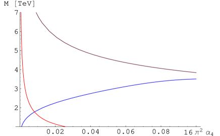
Figure 13: The allowed region for vector singlet resonances as function of $\alpha_{4}$ from the constraint $\lambda_{Z}$. The constraint from $\beta_{1}$, i.e. the $T$ parameter contribution from $\omega$ alone forces one to stay below the red line.

Since this is the only constraint at order $1/M^{2}$, it is by far dominant. As our main point is to point out what a measurement of the $\alpha$ parameter can do in unraveling the structure of electroweak symmetry breaking, we assumed that there is another contribution (e.g. a heavy scalar triplet) cancelling the $\omega$ contribution to $\beta_{1}$, and one is left with only terms of order $1/M^{4}$. The constraint from $T$ taken literally is shown in Fig. 13, showing that most of the allowed parameter range is cut out.

7.2.2 Vector Triplet: $\rho$

For the analysis of the vector triplet, we assume for simplicity that there is no mass splitting between the neutral and charged state of the resonance. As for the vector singlet, in the sequel we ignore the parameters $k_{\rho}$, $k^{\prime}_{\rho}$, and $k^{\prime\prime}_{\rho}$. To the order we are considering they do not contribute to the widths of the resonances,

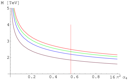
Figure 14: Dependence of the resonance mass for the vector triplet on ${\alpha}_{4}$ in the (quasi) isospin-conserving case $h_{\rho}=0$ ($g_{\rho}=0$) for different assumed widths (in red $f_{\rho}=\Gamma_{\rho}/M_{\rho}=1.0$, blue $0.8$,green $0.6$, brown $0.3$, respectively). All other parameters ($\mu$, $k$, $\ell$) are set to zero here. The red vertical line represents the $1\sigma$ limit for ${\alpha}_{4}$.

$f_{\rho}=\frac{\Gamma_{\rho}}{M_{\rho}}$	$1.0$	$0.8$	$0.6$	$0.3$
$M_{\rho}\ [{\rm TeV}]$	$2.49$	$2.36$	$2.19$	$1.84$

Table 15: Mass reach for the vector triplet if either $g_{\rho}=0$ or $h_{\rho}=0$ with all other parameters ($\ell$s, $k$s, $\mu$s) being zero, depending on different resonance widths.

and hence do not enter the electroweak fits at this stage. The same holds in principle for the coefficients of the magnetic moment operators of the heavy resonances, $\mu$ and $\mu^{\prime}$. As they are quantities with a more obvious physical interpretation we try to include them in the fits.

(i) As usual, we first consider isospin conservation, with only the parameters $\mu$, $g$, $\ell$ being nonzero. In principle, one could consider also $\mu^{\prime}$, $\ell^{\prime}$, and $k$ being nonzero, since in these terms isospin is only broken by hypercharge and not by any new physics effect. In this case, the relations among the parameters are quite simple:

$$\alpha_{1}=\;\alpha_{4}=-\alpha_{5}\quad\left(=-\alpha_{2}\right)$$ (100)

The equality in parentheses holds only for $\mu^{\prime}=k=0$. For the $\alpha^{\lambda}$s we have:

$$\alpha_{1}^{\lambda}=3\alpha_{3}^{\lambda}\quad\left(=-3\alpha_{2}^{\lambda}\right).$$ (101)

$\alpha_{2}^{\lambda}$ gets a correction when $\ell^{\prime}$ is switched on, and $\alpha_{4}^{\lambda}$ is not zero anymore then. For the masses, we get in the pure isospin-conserving case

$$M_{\rho}=v\left(\frac{12\pi\alpha_{4}f_{\rho}}{\alpha_{4}^{2}+2(\alpha_{2}^{\lambda})^{2}}\right)^{\frac{1}{4}},$$ (102)

while for $\ell^{\prime}$ switched on:

$$M_{\rho^{\pm}} =\;v\left(\frac{12\pi\alpha_{4}f_{\rho^{\pm}}}{\alpha_{4}^{2}+2(\alpha_{2}^{\lambda})^{2}+\frac{1}{2}\frac{s_{w}^{2}}{c_{w}^{2}}(\alpha_{4}^{\lambda})^{2}}\right)^{\frac{1}{4}}$$ (103a)

$$M_{\rho^{0}} =\;v\left(\frac{12\pi\alpha_{4}f_{\rho^{0}}}{\alpha_{4}^{2}+2(\alpha_{2}^{\lambda})^{2}}\right)^{\frac{1}{4}}.$$ (103b)

The case $\ell_{\rho}=0$ (i.e. $\alpha_{2}^{\lambda}=0$) seems to

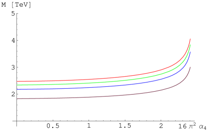
Figure 15: Dependence of the resonance mass for the vector triplet on ${\alpha}_{4}$ under the assumption $\ell_{\rho}=\ell^{\prime}_{\rho}=\ell^{\prime\prime}_{\rho}=0$ for different assumed widths: in red $f_{\rho}=\Gamma_{\rho}/M_{\rho}=1.0$, blue $0.8$, green $0.6$, brown $0.3$, respectively. On the left the neutral component is shown, on the right for charged one.

$f_{\rho}=\frac{\Gamma_{\rho}}{M_{\rho}}$	$1.0$	$0.8$	$0.6$	$0.3$
$M_{\rho^{\pm}}\ [{\rm TeV}]$	$2.67$	$2.53$	$2.35$	$1.98$
$M_{\rho^{0}}\ [{\rm TeV}]$	$1.74$	$1.65$	$1.53$	$1.29$

Table 16: Mass reach for the vector triplet under the assumption $\ell_{\rho}=\ell^{\prime}_{\rho}=\ell^{\prime\prime}_{\rho}=0$. Values for the charged component are averaged over the lower limit.

bring one back to the corresponding case for the vector singlet. But now the correlations among the parameters are different, especially $\alpha_{6}$ and $\alpha_{7}$ are zero here but not in the singlet case. Note also, that the assumption $g_{\rho}=0$, $h_{\rho}\neq 0$ leads to the same result, as the formulas for the width and the functional dependence of the $\alpha$s on the coupling change in the same manner. The mass reach for the vector triplet in this case is shown in Fig. 14 and Table 15.

(ii) Taking into account isospin violation, we note that the following relations hold generally among the $\alpha$ and $\alpha^{\lambda}$ parameters

$$\alpha_{4} =\;-\alpha_{5} \alpha_{6} =\;-\alpha_{7}$$ (104a)

$$\alpha_{1} =\;\alpha_{4}+\alpha_{6} \alpha_{8} =\;-\frac{\alpha_{6}}{2}\left(1+\frac{\alpha_{6}}{2(\sqrt{\alpha_{1}}+\sqrt{\alpha_{4}})^{2}}\right)\;\;.$$ (104b)

And among the $\alpha^{\lambda}$s:

$$2(\alpha_{1}^{\lambda}+\alpha_{2}^{\lambda}) =\;-\left(1+\sqrt{\frac{\alpha_{1}}{\alpha_{4}}}\right)(2\alpha_{3}^{\lambda}+\alpha_{4}^{\lambda})$$ (105a)

We first consider the special case $g_{\rho}=-h_{\rho}$ where the $\beta_{1}$ ($T$ parameter) vanishes (we neglect a possible $\Delta M_{\rho}$). To simplify things, we first set all the $k$s and $\ell$s to zero. Then, (104a) simplifies to

$$\alpha_{1}=\frac{1}{3}\alpha_{2}=-\alpha_{3}=\frac{1}{9}\alpha_{4}=-\frac{1}{8}\alpha_{6}=\frac{1}{2}\alpha_{9}.$$ (106)

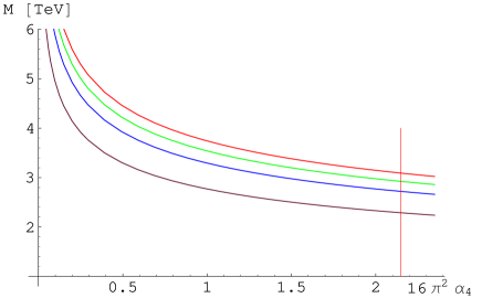
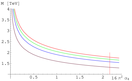
Figure 16: Dependence of the resonance mass for the vector triplet on $\alpha_{4}$ in the special isospin-violating case $g_{\rho}=-h_{\rho}$ for different assumed width to mass ratios (in red $f_{\rho}=\Gamma_{\rho}/M_{\rho^{+}}=1.0$, blue $0.8$,green $0.6$, brown $0.3$, respectively). On the left is the charged resonance, on the right the neutral one.

$f_{\rho}=\frac{\Gamma_{\rho}}{M_{\rho}}$	$1.0$	$0.8$	$0.6$	$0.3$
$M_{\rho^{\pm}}\ [{\rm TeV}]$	$3.09$	$2.92$	$2.72$	$2.29$
$M_{\rho^{0}}\ [{\rm TeV}]$	$1.78$	$1.69$	$1.57$	$1.32$

Table 17: Mass reach for the vector triplet in the special isospin-violating case $g_{\rho}=-h_{\rho}$.

For this special isospin-violating case, the formulas for the masses of the resonances are:

$$M_{\rho^{\pm}} =\;v\left(\frac{108\pi f_{\rho^{\pm}}}{\alpha_{4}}\right)^{\frac{1}{4}}$$ (107a)

$$M_{\rho^{0}} =\;v\left(\frac{12\pi f_{\rho^{0}}}{\alpha_{4}}\right)^{\frac{1}{4}}$$ (107b)

The dependence of the mass of the vector resonance in this case is shown in Fig. 16, and the mass reach in Table 17. Note that the difference between the charged and the neutral state is just the factor $\sqrt{3}$ from (107).

Next, we still assume $g_{\rho}=-h_{\rho}$ and hence no contribution to the $T$ parameter, but allow for nonzero values of

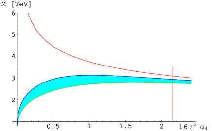
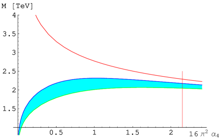
Figure 17: Dependence of the resonance mass for the charged component of the vector triplet on ${\alpha}_{4}$ for different assumed widths (f=1 on the left and f=0.3 on the right) for $g=-h$ case, but $\ell_{\rho},\ell^{\prime}_{\rho}\neq 0$. The red and blue line are the lower and upper limit from $\lambda_{Z}$, respectively. Vertical red line: maximal allowed value of ${\alpha}_{4}$. The blue shaded area is the allowed one when $\mu_{\rho},\mu^{\prime}_{\rho}\neq 0$.

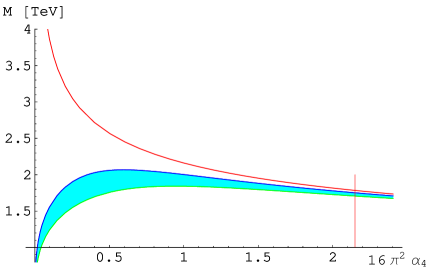
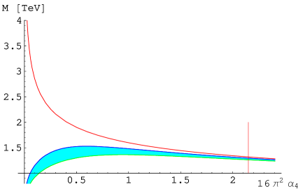
Figure 18: Same as Fig. 17, but for the neutral component.

$f_{\rho}=\frac{\Gamma_{\rho}}{M_{\rho}}$	$1.0$	$0.8$	$0.6$	$0.3$
$M_{\rho^{\pm}}\ [{\rm TeV}]$	$2.91$	$2.75$	$2.56$	$2.16$
$M_{\rho^{0}}\ [{\rm TeV}]$	$1.84$	$1.79$	$1.66$	$1.40$

Table 18: Mass reach for the vector triplet under the assumption $g_{\rho}=-h_{\rho}$ with nonzero $\ell_{\rho}$s. The values in the table are average values along the lower limit curve.

$\ell_{\rho}$ and $\ell^{\prime}_{\rho}$. In complete analogy to the discussion for the vector singlet, we now have to include the measurements of the triple gauge couplings to access $\lambda_{Z}$ and $\lambda_{\gamma}$ in order to have enough equations at hand to solve the system, which is fulfilled if one of the $\ell_{\rho}$s is set to zero. We take $\ell^{\prime\prime}_{\rho}\equiv 0$. Taking the allowed range of $0\lesssim\lambda_{Z}\lesssim 0.00033$ from [41], we again get an upper and a lower limiting curve for $M_{\rho}$ as a function of $\alpha_{4}$. The allowed range is in between. The situation is shown in Fig. 17 for the charged state, and in

$f_{\rho}=\frac{\Gamma_{\rho}}{M_{\rho}}$	$1.0$	$0.8$	$0.6$	$0.3$
$M_{\rho^{\pm}}\ [{\rm TeV}]$	$2.54$	$2.41$	$2.34$	$1.88$
$M_{\rho^{0}}\ [{\rm TeV}]$	$1.71$	$1.62$	$1.51$	$1.27$

Table 19: Mass reach for the vector triplet with the assumptions $g_{\rho}=-h_{\rho}$ with nonvanishing $\ell_{\rho},\ell^{\prime}_{\rho}$ and nonvanishing $\mu_{\rho},\mu^{\prime}_{\rho}$. The values in the table are average values along the lower limit curve.

Fig. 18 for the neutral one. The mass reach for this choice of parameters is given in Table 18.

As a next step, we still assume $g_{\rho}=-h_{\rho}$, but allow for nonvanishing $\mu_{\rho}$ and $\mu^{\prime}_{\rho}$. This offers the possibility of various cancellations among the different parameters, especially since the $\mu$s enter linearly in the $\alpha$s and can have arbitrary sign. This fact completely cancels the gain in using a new constraint on the system, and so the bound for the vector resonance mass losens a bit. The allowed parameter regions are shown as blue shadings in Fig. 17 for the charged and in Fig. 18 for the neutral state, respectively. The mass reach is shown in Table 19.

Considering all isospin-violating terms, there are now (still ignoring the $k$s) all $\alpha$ and $\alpha^{\lambda}$ parameters nonvanishing, except for $\alpha_{10}$. The masses of the resonances are then:

$$M_{\rho^{\pm}} =\;v\left(\frac{12\pi\alpha_{1}f_{\rho^{\pm}}}{\alpha_{1}^{2}+2(\alpha^{\lambda}_{3})^{2}+\frac{1}{2}\frac{s_{w}^{2}}{c_{w}^{2}}(\alpha_{4}^{\lambda})^{2}}\right)^{\frac{1}{4}}$$ (108a)

$$M_{\rho^{0}} =\;v\left(\frac{12\pi\alpha_{4}f_{\rho^{0}}}{\alpha_{4}^{2}+2\left(\alpha_{3}^{\lambda}\sqrt{\frac{\alpha_{4}}{\alpha_{1}}}+2\alpha_{5}^{\lambda}\right)^{2}}\right)^{\frac{1}{4}}$$ (108b)

Allowing for arbitrary variations of $g_{\rho}$ and $h_{\rho}$ and taking non-zero values for the $\ell_{\rho}$, $k_{\rho}$ and $\mu_{\rho}$ parameters into account, one again has to use the results from [41] to access $\lambda_{\gamma}$ and $\lambda_{Z}$ from the measurements of the triple gauge couplings. However we found that the (independent) variation of $g_{\rho}$ and $h_{\rho}$ already introduces enough freedom into the system so that allowing for nonzero values for the other parameters does not extend the allowed region in $(\alpha_{4},M_{\rho})$ parameter space significantly. Hence, the allowed region shows up only as tiny bands below the corresponding curves in Figure 15. The limits for the mass reach given in Table 16 do therefore not change significantly.

7.3 $J=2$ Channel

7.3.1 Tensor Singlet: $f$

(i) For conserved isospin, $\alpha_{4}$ and $\alpha_{5}$ are non-zero, but related to each other by the constraint

Figure 19: Dependence of the resonance mass for the tensor singlet case on ${\alpha}_{4}$ for different assumed width to mass ratios ($f_{f}=\Gamma_{f}/M_{f}=1.0$ in red, $0.8$ in blue, $0.6$ in green, and $0.3$ in brown, respectively). The red vertical line represents the $1\,\sigma$ limit for ${\alpha}_{4}$.

$$\alpha_{5}=-\frac{1}{4}\alpha_{4}.$$ (109)

$f_{f}=\frac{\Gamma_{f}}{M_{f}}$	$1.0$	$0.8$	$0.6$	$0.3$
$M_{f}\ [{\rm TeV}]$	$3.29$	$3.11$	$2.89$	$2.43$

Table 20: Mass reach for the tensor singlet in the $SU(2)_{c}$ conserving case depending on different resonance widths.

From the fit we get ${\alpha}_{4}=0.64369$ for the parabolic error and $-0.65404<{\alpha}_{4}<0.62154$ for the asymmetric errors at $1\,\sigma$ level.

The mass of a singlet tensor resonance is then given by

$$M_{f}=v\left(\frac{40\pi f_{f}}{\alpha_{4}}\right)^{\frac{1}{4}}.$$ (110)

(ii) If we allow for isospin breaking, also $\alpha_{6}$, $\alpha_{7}$ and $\alpha_{10}$ are non-zero, but subjected to the two constraints

$$\alpha_{7}=-\frac{1}{4}\alpha_{6},\qquad\alpha_{7}^{2}=-\frac{2}{3}\alpha_{5}\alpha_{10}\;\;\left[\text{or}\;\;\alpha_{6}^{2}=\frac{8}{3}\alpha_{4}\alpha_{10}\right],$$ (111)

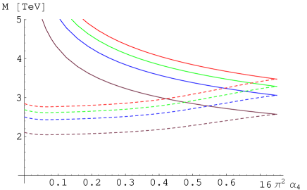
Figure 20: Dependence of the resonance mass for the tensor singlet with broken isospin on ${\alpha}_{4}$ for different assumed width to mass ratios: $f_{f}=\Gamma_{f}/M_{f}=1.0$ (red), $0.8$ (blue), $0.6$ (green), and $0.3$ (brown), respectively. Along the $1\,\sigma$ contour, the lower limit is given by the dashed line, while the full line is the upper limit.

$f_{f}=\frac{\Gamma_{f}}{M_{f}}$	$1.0$	$0.8$	$0.6$	$0.3$
$M_{f}\ [{\rm TeV}]$	$3.00$	$2.84$	$2.64$	$2.22$

Table 21: Mass reach for the tensor singlet in the broken isospin case depending on different resonance widths.Values in the table are average values along the lower limit.

while the former relation (109) still holds. We choose to take $\alpha_{4}$ and $\alpha_{6}$ as independent parameters. Then the mass of the tensor singlet is given by

$$M_{f}=v\left(\frac{120\pi\alpha_{4}f_{f}}{2\alpha_{4}^{2}+(\alpha_{4}+\alpha_{6})^{2}}\right)^{\frac{1}{4}}.$$ (112)

The maximum for the resonance mass is reached when we set $\alpha_{4}=-\alpha_{6}$, leaving us with a one-parameter fit. The maximal mass is given by $M_{f,max}=v\left(60\pi f_{f}/\alpha_{4}\right)^{\frac{1}{4}}$, leading to the upper bound in Fig. 20.

7.3.2 Tensor Triplet: $a$

(i) Like for the triplet scalar, a tensor triplet as a resonance can only occur with the help of isospin breaking. Again, we consider the case $h_{a}=k_{a}=0$, so that $h^{\prime}_{a}$ is the only non-vanishing parameter. In that case, isospin breaking does not show up experimentally, as only $\alpha_{4}=-4\alpha_{5}$ is non-zero. Like in the scalar case, the charged resonance decouples, while for the mass we get the same relation as in the singlet case:

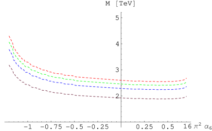
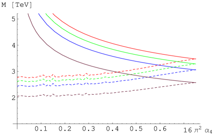
Figure 21: Mass reach for tensor triplet resonances with isospin breaking for different assumed width to mass ratios, $f_{a}=\Gamma_{a}/M_{a}=1.0$ (red), $0.8$ (blue), $0.6$ (green), $0.3$ (brown), respectively. On the left: the charged components, on the right: neutral component. Full/dashed line: upper/lower limit within the $1\,\sigma$ contour.

$f_{a}=\frac{\Gamma_{a}}{M_{a}}$	$1.0$	$0.8$	$0.6$	$0.3$
$M_{a^{0}}\,[{\rm TeV}]$	$3.01$	$2.85$	$2.65$	$2.23$
$M_{a^{\pm}}\,[{\rm TeV}]$	$2.81$	$2.66$	$2.47$	$2.08$

Table 22: Dependence of the mass reach for tensor triplet resonances on different resonance widths. For the neutral component, the numbers in the table are average values along the lower limit contour.

$$M_{a^{0}}=v\left(\frac{40\pi f_{a^{0}}}{\alpha_{4}}\right)^{\frac{1}{4}}$$ (113)

The fit (and hence the limits) is identical to the isospin-conserving case of the tensor singlet.

(ii) In the most general isospin-breaking case, we have five possibly nonvanishing parameters $\alpha_{i}$ for $i=4,5,6,7,10$ and two independent masses. There are two constraints among the parameters, namely

$$\alpha_{5} =\;-\frac{1}{4}\alpha_{4}$$ (114a)

$$(2\alpha_{6}-\alpha_{7})^{2} =\;\frac{9}{2}\alpha_{4}\left(\alpha_{6}+4\alpha_{7}+3\alpha_{10}\right)$$ (114b)

Solving for the masses of the resonances, yields the formulas:

$$M_{a^{\pm}} =\;v\left(\frac{270\pi f_{a^{\pm}}}{\alpha_{6}+4\alpha_{7}}\right)^{\frac{1}{4}}$$ (115a)

$$M_{a^{0}} =\;v\left(\frac{120\pi\alpha_{4}f_{a^{0}}}{2\alpha_{4}^{2}+(\alpha_{4}+\frac{8}{9}\alpha_{6}-\frac{4}{9}\alpha_{7})^{2}}\right)^{\frac{1}{4}}$$ (115b)

The denominator for the neutral component is minimized within the $1\,\sigma$ volume on the surface defined by $9\alpha_{4}+8\alpha_{6}-4\alpha_{7}=0$. This is equivalent to the condition $h_{a}+h^{\prime}_{a}+2k_{a}=0$, and maximizes the mass of the neutral state to become $M_{a^{0}}=v\left(60\pi f_{a^{0}}/\alpha_{4}\right)^{\frac{1}{4}}$.

7.3.3 Tensor Quintet: $t$

(i) For the tensor quintet, there is the case of strict isospin conservation, where only $\alpha_{4}$ and $\alpha_{5}$ are nonvanishing with the constraint $\alpha_{5}=2\alpha_{4}$. This degeneracy is lifted as soon as the isospin breaking coupling $h^{\prime}$ is switched on. Solving for the mass yields

$$M_{t}=v\left(\frac{30\pi f_{t}}{\alpha_{4}}\right)^{\frac{1}{4}}$$ (116)

There are four other cases, in which also only the isospin-conserving parameters $\alpha_{4,5}$ are non-zero and experimentally isospin breaking cannot be measured. This can either be achieved by having $h^{\prime}_{t}\neq 0$ and all other parameters vanishing or $h^{\prime}_{t}$ vanishing. In the second case, the relation $\alpha_{5}=2\alpha_{4}$ again holds.

• Only the coupling $h^{\prime}_{t}$ is switched on (which is special in the sense that at least the SM part couples to a singlet invariantly). Here the charged resonances decouple, and for the neutral we get:

  $$M_{t^{0}}=\;v\left(\frac{60\pi f_{t^{0}}}{\alpha_{4}}\right)^{\frac{1}{4}}.$$ (117)

• $h^{\prime}_{t}=h_{t}=0$, $g_{t}=-2k_{t}$:

• $h^{\prime}_{t}=0$, $g_{t}=k_{t}=-\frac{1}{2}h_{t}$:

• $h^{\prime}_{t}=0$, $g_{t}=2k_{t}=-\frac{1}{2}h_{t}$:

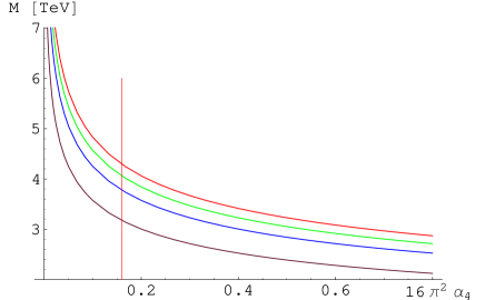
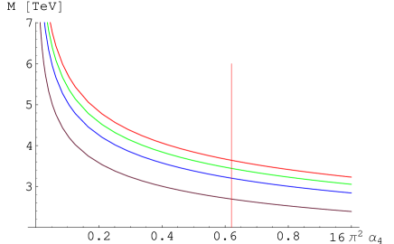
Figure 22: Dependence of the resonance mass for the tensor quintet on ${\alpha}_{4}$ for different assumed widths (in red $f_{t^{0}}=\Gamma_{t^{0}}/M_{t0}=1.0$, blue $0.8$,green $0.6$, brown $0.3$). The red vertical line represents the $1\sigma$ limit for ${\alpha}_{4}$. On the left: Isospin-conserving case and isospin-breaking cases b),c),and d) described in the text. On the right: isospin-breaking case a).

$f=\frac{\Gamma}{M_{t}}$	$1.0$	$0.8$	$0.6$	$0.3$
$M_{t}\ [{\rm TeV}]$	$4.30$	$4.06$	$3.78$	$3.18$

$f=\frac{\Gamma}{M_{t}}$	$1.0$	$0.8$	$0.6$	$0.3$
$M_{t}\ [{\rm TeV}]$	$3.64$	$3.44$	$3.20$	$2.69$

Table 23: Mass reach for the tensor quintet: On the left in the $SU(2)_{c}$ conserving case as well as for the cases b), c), and d) described in the text, depending on different resonance widths. On the right, case a) where only $h^{\prime}_{t}\neq 0$.

In all the cases b) to d), the neutral, charged and doubly charged resonances are degenerate in mass, and we get

$$M_{t}=\;v\left(\frac{30\pi f_{t}}{\alpha_{4}}\right)^{\frac{1}{4}}.$$ (118)

So for the experimental sensitivity, the cases b) to d) are equivalent to the strictly isospin-conserving case. Here, from the fit we obtain $\delta\alpha_{4}=0.16116$ as a parabolic error and $-0.17387<\alpha_{4}<0.15134$ as asymmetric ones at $1\,\sigma$.

A next case would be to consider only $g_{t}$ and $h^{\prime}_{t}$ different from zero. In that case only $\alpha_{10}$ vanishes, while we have the two constraints

$$\alpha_{7}=-\frac{1}{4}\alpha_{6},\qquad\alpha_{6}^{2}=\frac{16}{81}(2\alpha_{4}-\alpha_{5})(\alpha_{4}+4\alpha_{5}).$$ (119)

So here, experimentally we can measure isospin breaking in the resonance sector. For the masses of the tensor resonances, there

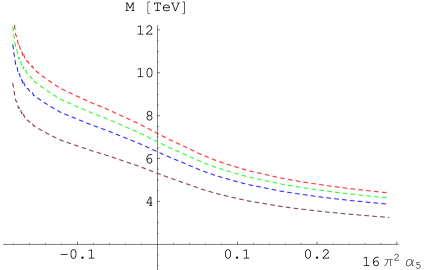
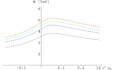
Figure 23: Dependence of the resonance mass for the tensor quintet in special case $h=k=0$ for different assumed widths (in red $f=\Gamma/M_{t}=1.0$, blue $0.8$,green $0.6$, brown $0.3$)

$f=\frac{\Gamma}{M_{t}}$	$1.0$	$0.8$	$0.6$	$0.3$
$M_{t^{c}}\ [{\rm TeV}]$	$6.76$	$6.39$	$5.95$	$5.00$
$M_{t^{0}}\ [{\rm TeV}]$	$4.53$	$4.28$	$3.98$	$3.35$

Table 24: Mass reach for the tensor quintet in the $h=k=0$ case depending on different resonance widths.Values in the table are average over lower limit.

is a splitting between the neutral and the charged ones ($t^{c}=t^{\pm},t^{\pm\pm}$):

$$M_{t^{c}} =\;v\left(\frac{270\pi f_{t^{c}}}{\alpha_{4}+4\alpha_{5}}\right)^{\frac{1}{4}}$$ (120a)

$$M_{t^{0}} =\;v\left(\frac{270\pi f_{t^{0}}}{5\alpha_{4}+2\alpha_{5}}\right)^{\frac{1}{4}}$$ (120b)

The mass reach in this case is shown in Fig. 23 as well as Table 24.

(ii) For the completely general case, all couplings are non-zero, and the constraint equation is

$$(2\alpha_{6}-\alpha_{7})^{2}=(2\alpha_{4}-\alpha_{5})\left(\alpha_{4}+4\alpha_{5}+2\alpha_{6}+8\alpha_{7}+6\alpha_{10}\right).$$ (121)

The masses for the tensor quintet are (we use the abbreviations

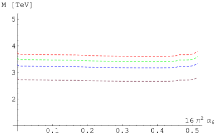
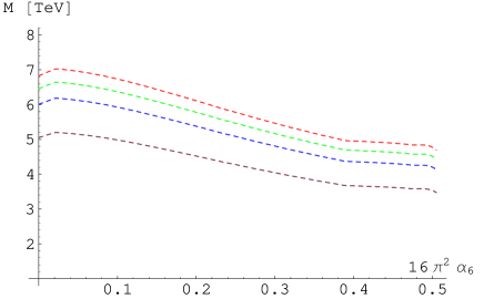
Figure 24: Dependence of the resonance mass for the tensor quintet in the full case for different assumed widths (in red $f_{t}=\Gamma_{t}/M_{t}=1.0$, blue $0.8$,green $0.6$, brown $0.3$, respectively). On the upper line, the doubly charged case is shown on the left, the charged one on the right, while the neutral state is in the lower line.

$f=\frac{\Gamma}{M_{t}}$	$1.0$	$0.8$	$0.6$	$0.3$
$M_{t^{\pm\pm}}\ [{\rm TeV}]$	$5.17$	$4.89$	$4.55$	$3.83$
$M_{t^{\pm}}\ [{\rm TeV}]$	$3.64$	$3.44$	$3.20$	$2.69$
$M_{t^{0}}\ [{\rm TeV}]$	$5.84$	$5.52$	$5.14$	$4.32$

Table 25: Mass reach for the tensor quintet in the full case depending on different resonance widths. The values given in the table are averaged over the lower limit curve.

$\xi_{ij}=\alpha_{i}+4\alpha_{j}$):

$$M_{t^{\pm\pm}} =\;v\left(\frac{270\pi f_{t^{\pm\pm}}}{\xi_{45}}\right)^{\frac{1}{4}}$$ (122a)

$$M_{t^{\pm}} =\;v\left(\frac{270\pi f_{t^{\pm}}}{\xi_{45}+\xi_{67}}\right)^{\frac{1}{4}}$$ (122b)

$$M_{t^{0}} =\;v\left(\frac{810\pi(2\alpha_{4}-\alpha_{5})f_{t^{0}}}{\left[\sqrt{(\alpha_{4}+4\alpha_{5})(2\alpha_{4}-\alpha_{5})}-2(2\alpha_{4}-\alpha_{5})\right]^{2}+2\left[2(\alpha_{4}+\alpha_{6})-(\alpha_{5}+\alpha_{7})\right]^{2}}\right)^{\frac{1}{4}}$$

$$=\;v\left(\frac{810\pi f_{t^{0}}}{\left[\sqrt{\xi_{45}}-2\sqrt{2\alpha_{4}-\alpha_{5}}\right]^{2}+2\left[\sqrt{2\alpha_{4}-\alpha_{5}}+\sqrt{\xi_{45}+2\xi_{67}+6\alpha_{10}}\right]^{2}}\right)^{\frac{1}{4}}$$ (122c)

For the neutral component, the first formula is better suited for the fit, while the limit to the isospin-conserving case is easily visible in the second one as well as the limit to the special case above with $\xi_{67}\to 0$ for only $g_{t}$ and $h^{\prime}_{t}$ being non-zero.

8 Summary

At an ILC with high energy ($1\;{\rm TeV}$) and luminosity ($1000\;{\rm fb}^{-1}$) and the possibility for both electron and positron polarization, precise measurements of weak-boson interactions will be feasible. In this work we have concentrated on quartic weak-boson couplings that enter in six-fermion processes. Including known results for weak-boson pair production and oblique corrections, we have determined the possible impact on our knowledge about high-energy weak-boson scattering amplitudes. Our numerical results are presented in terms of the usual set of anomalous couplings in the chiral-Lagrangian framework. For each spin-isospin channel, they are conveniently re-expressed in terms of the maximal resonance mass that, under the most favorable conditions, the measurement can be sensitive to.

On the experimental side, the present study completes and supersedes previous studies of weak-boson scattering and triple-boson production in $e^{+}e^{-}$ collisions. For weak-boson scattering processes, we have analysed all accessible channels using an unweighted event generator with complete six-fermion matrix elements, parton shower and hadronization, and fast detector simulation. The analysis uses standard cut-based experimental techniques. The parameters are determined in a global multidimensional fit without implicit or explicit assumptions of theoretical relations among them.

Triple weak-boson production provides independent information on the parameters of interest. While our results indicate that the ultimate sensitivity is not as good as for the weak-boson scattering processes, it serves as an important cross check and should be included in a global fit of ILC data. More details on this class of processes will be published elsewhere [46].

In Tables 26, 27 we combine our results for the physics sensitivity for all spin/isospin channels. Table 26 assumes $SU(2)_{c}$ conservation, so the $\Delta\rho$ parameter automatically vanishes. In this case, only channels with $I+J$ even couple to weak-boson pairs. Table 27 shows the results without this constraint. In each case, a single resonance with maximal coupling (i.e., $\Gamma=M$) was assumed to be present. In a real situation, the particular structure of the parameter dependence can be used to disentangle multiple resonances.

$$\begin{array}[]{|c||c|c|c|}\hline\cr\text{Spin}&I=0&I=1&I=2\\ \hline\cr\hline\cr 0&1.55&-&1.95\\ 1&-&2.49&-\\ 2&3.29&-&4.30\\ \hline\cr\end{array}$$

Table 26: Accessible scale $\Lambda$ in ${\rm TeV}$ for all possible spin/isospin channels. The results are derived from the analysis of vector-boson scattering processes at the ILC, assuming a single resonance with optimal properties. Custodial $SU(2)$ symmetry is assumed to hold.

$$\begin{array}[]{|c||c|c|c|}\hline\cr\text{Spin}&I=0&I=1&I=2\\ \hline\cr\hline\cr 0&1.39&1.55&1.95\\ 1&1.74&2.67&-\\ 2&3.00&3.01&5.84\\ \hline\cr\end{array}$$

Table 27: Accesible scale $\Lambda$ in ${\rm TeV}$ for all possible spin/isospin channels. The results are derived from the analysis of vector-boson scattering processes at the ILC, assuming a single resonance with optimal properties. No constraints beyond the SM symmetries are assumed.

Some important properties of the relation of resonances to anomalous couplings are worth mentioning. First of all, we have to distinguish resonances that (in our operator basis) couple to fermions from those that do not. If sizable fermion couplings are present, some anomalous couplings scale with $1/M^{2}$, where $M$ is the resonance mass. Obviously, these include four-fermion contact terms, which are thus potentially sensitive to new-physics up to rather high scales. The other class of operators with $1/M^{2}$ scaling are mixed fermion-boson contact terms that contribute, e.g., to vector boson pair production. In any fixed operator basis, these operators are not related to the triple-gauge interactions that are usually considered. However, in studies that deal with specific models (e.g., minimal technicolor), they are implicitly present. This accounts for the good physics reach of the ILC as it has been discovered in studies of weak-boson pair production.

In this work, we have determined the amount of information that can possibly be gained on top of the analysis of fermionic couplings, or otherwise if such couplings are small or absent. In that case, the only operator with a physical $1/M^{2}$ scaling corresponds to the $\rho$ parameter, associated to custodial-$SU(2)$ violation. Apart from that, all $1/M^{2}$ effects in bosonic interactions can be absorbed into unobservable redefinitions of the SM parameters. Therefore, the shifts due to heavy resonances in oblique corrections, triple-gauge couplings, and quartic gauge couplings, all scale with $1/M^{4}$. In particular, all corrections to triple-gauge couplings ($g,\kappa,\lambda$) scale in the same way, although the operators have formally different dimension.

Taking these considerations into account, we find limits for the sensitivity of the ILC in the $1$ to $3~{}{\rm TeV}$ range, where the best reach corresponds to the highest-spin channel. These limits are not as striking as possible limits from contact interactions, but agree well with the expected direct-search limits for resonances at the LHC. Performing global fits of all electroweak parameters, analogous to LEP analyses, and combining data from both colliders will be important for disentangling the contributions. Significant knowledge about the mechanism of electroweak symmetry breaking can thus be gained even in ‘worst-case’ scenarios that do not lead to striking new-physics signatures at all.

Acknowledgments

We would like to thank Peter Zerwas for useful comments and discussions. W.K. and J.R. are supported by the Helmholtz-Gemeinschaft, Contract No. VH–NG–005.

Appendix A Chiral Parameters and Anomalous Couplings

In this section, we list the formulas that relate the operators of the chiral Lagrangian (see Sec. 2) to the anomalous couplings of vector bosons in the physical basis of $A_{\mu}$, $Z_{\mu}$, $W^{\pm}_{\mu}$. While standard parameterizations exist for the oblique corrections and for the triple gauge couplings (TGC), this is not the case for quartic anomalous couplings.

A.1 Oblique corrections

New physics that does not couple to light fermions can be parameterized in terms of $S,T,U$. The relations are

$$\Delta S =-16\pi\alpha_{1} \Delta T =2\beta_{1}/{\alpha_{\rm QED}} \Delta U =-16\pi\alpha_{8}$$ (123)

The oblique corrections are needed for the proper renormalization of the SM vertices. First, we have to specify our definition of the weak mixing angle. It is customary to adopt the $G_{F}/\alpha/M_{Z}$ scheme. In this scheme, the weak mixing angle is defined by

$$s_{w}c_{w}=\frac{e}{2M_{Z}}(\sqrt{2}G_{F})^{-1/2}.$$ (124)

Furthermore, the oblique corrections renormalize the wave functions of the vector bosons and thus affect the definition of the gauge couplings $g$ and $g^{\prime}$ in terms of $e$ and $s_{w},c_{w}$.

A simple recipe of including the oblique corrections to the trilinear and quartic gauge couplings is the following: (i) Expand the SM Lagrangian in terms of physical fields according to

$$gW^{3}=eA+e\frac{c_{w}}{s_{w}}(1+\delta_{Z})Z,\qquad\qquad gW^{\pm}=\frac{e}{s_{w}}\left(1+c_{w}^{2}\delta_{Z}-\frac{g^{2}}{2}\alpha_{8}\right)W^{\pm}$$ (125)

where

$$\delta_{Z}=\frac{\beta_{1}+g^{\prime\,2}\alpha_{1}}{c_{w}^{2}-s_{w}^{2}},$$ (126)

and (ii) switch to the $G_{F}/\alpha/M_{Z}$ scheme by the replacements

$$s_{w} \to s_{w}\left(1-\frac{c_{w}^{2}}{c_{w}^{2}-s_{w}^{2}}\beta_{1}-\frac{e^{2}}{2s_{w}^{2}(c_{w}^{2}-s_{w}^{2})}\alpha_{1}\right)$$ (127)

$$c_{w} \to c_{w}\left(1+\frac{s_{w}^{2}}{c_{w}^{2}-s_{w}^{2}}\beta_{1}+\frac{e^{2}}{2c_{w}^{2}(c_{w}^{2}-s_{w}^{2})}\alpha_{1}\right)$$ (128)

A.2 Triple gauge couplings

We define a generic $C$ and $CP$-even triple-gauge vertex in the standard way

$$\mathcal{L}_{TGC} =\mathrm{i}e\left[g_{1}^{\gamma}A_{\mu}\left(W^{-}_{\nu}W^{+\mu\nu}-W^{+}_{\nu}W^{-\mu\nu}\right)+\kappa^{\gamma}W^{-}_{\mu}W^{+}_{\nu}A^{\mu\nu}+\frac{\lambda^{\gamma}}{M_{W}^{2}}W^{-}_{\mu}{}^{\nu}W^{+}_{\nu\rho}A^{\rho\mu}\right]$$

$$\quad+\mathrm{i}e\frac{c_{w}}{s_{w}}\left[g_{1}^{Z}Z_{\mu}\left(W^{-}_{\nu}W^{+\mu\nu}-W^{+}_{\nu}W^{-\mu\nu}\right)+\kappa^{Z}W^{-}_{\mu}W^{+}_{\nu}Z^{\mu\nu}+\frac{\lambda^{Z}}{M_{W}^{2}}W^{-}_{\mu}{}^{\nu}W^{+}_{\nu\rho}Z^{\rho\mu}\right]$$ (129)

The SM values are

$$g_{1}^{\gamma,Z}=\kappa^{\gamma,Z}=1\quad\text{and}\quad\lambda^{\gamma,Z}=0$$ (130)

The triple gauge couplings are expressed in terms of the $\alpha$ parameters as

$$\Delta g_{1}^{\gamma} =0 \Delta\kappa^{\gamma} =g^{2}(\alpha_{2}-\alpha_{1})+g^{2}\alpha_{3}+g^{2}(\alpha_{9}-\alpha_{8})$$ (131)

$$\Delta g_{1}^{Z} =\delta_{Z}+\frac{g^{2}}{c_{w}^{2}}\alpha_{3} \Delta\kappa^{Z} =\delta_{Z}-g^{\prime\,2}(\alpha_{2}-\alpha_{1})+g^{2}\alpha_{3}+g^{2}(\alpha_{9}-\alpha_{8})$$ (132)

and

$$\lambda^{\gamma} =-\frac{g^{2}}{2}\left(\alpha^{\lambda}_{1}+\alpha^{\lambda}_{2}\right) \lambda^{Z} =-\frac{g^{2}}{2}\left(\alpha^{\lambda}_{1}-\frac{s_{w}^{2}}{c_{w}^{2}}\alpha^{\lambda}_{2}\right)$$ (133)

where $\delta_{Z}$ is the oblique correction defined above.

This can be inverted to yield

$$\alpha_{2}-\alpha_{1} =\frac{c_{w}^{2}}{g^{2}}(\Delta\kappa^{\gamma}-\Delta\kappa^{Z}+\delta_{Z})$$ (134)

$$\alpha_{3} =\frac{c_{w}^{2}}{g^{2}}\left(\Delta g_{1}^{Z}-\delta_{Z}\right)$$ (135)

$$\alpha_{9}-\alpha_{8} =\frac{s_{w}^{2}}{g^{2}}\Delta\kappa^{\gamma}+\frac{c_{w}^{2}}{g^{2}}(\Delta\kappa^{Z}-\Delta g_{1}^{Z})$$ (136)

$$\alpha^{\lambda}_{1} =-\frac{2}{g^{2}}\left(s_{w}^{2}\lambda^{\gamma}+c_{w}^{2}\lambda^{Z}\right)$$ (137)

$$\alpha^{\lambda}_{2} =-\frac{2}{g^{2}}\,c_{w}^{2}\left(\lambda^{\gamma}-\lambda^{Z}\right)$$ (138)

A.3 Quartic gauge couplings

We define the quartic gauge couplings analogous to the TGC:

$$\mathcal{L}_{QGC} =e^{2}\left[g_{1}^{\gamma\gamma}A^{\mu}A^{\nu}W^{-}_{\mu}W^{+}_{\nu}-g_{2}^{\gamma\gamma}A^{\mu}A_{\mu}W^{-\nu}W^{+}_{\nu}\right]$$

$$\quad+e^{2}\frac{c_{w}}{s_{w}}\left[g_{1}^{\gamma Z}A^{\mu}Z^{\nu}\left(W^{-}_{\mu}W^{+}_{\nu}+W^{+}_{\mu}W^{-}_{\nu}\right)-2g_{2}^{\gamma Z}A^{\mu}Z_{\mu}W^{-\nu}W^{+}_{\nu}\right]$$

$$\quad+e^{2}\frac{c_{w}^{2}}{s_{w}^{2}}\left[g_{1}^{ZZ}Z^{\mu}Z^{\nu}W^{-}_{\mu}W^{+}_{\nu}-g_{2}^{ZZ}Z^{\mu}Z_{\mu}W^{-\nu}W^{+}_{\nu}\right]$$

$$\quad+\frac{e^{2}}{2s_{w}^{2}}\left[g_{1}^{WW}W^{-\mu}W^{+\nu}W^{-}_{\mu}W^{+}_{\nu}-g_{2}^{WW}\left(W^{-\mu}W^{+}_{\mu}\right)^{2}\right]+\frac{e^{2}}{4s_{w}^{2}c_{w}^{4}}h^{ZZ}(Z^{\mu}Z_{\mu})^{2}$$ (139)

The SM values are

$$g_{1}^{VV^{\prime}}=g_{2}^{VV^{\prime}}=1\quad\text{($VV^{\prime}=\gamma\gamma,\gamma Z,ZZ,WW$),}\qquad\qquad h^{ZZ}=0.$$ (140)

In terms of the $\alpha$ parameters, the deviations from the SM values are

$$\Delta g_{1}^{\gamma\gamma} =\Delta g_{2}^{\gamma\gamma}=0 =\Delta g_{1}^{\gamma}$$ (141)

$$\Delta g_{1}^{\gamma Z} =\Delta g_{2}^{\gamma Z}=\delta_{Z}+\frac{g^{2}}{c_{w}^{2}}\alpha_{3} =\Delta g_{1}^{Z}$$ (142)

$$\Delta g_{1}^{ZZ} =2\Delta g_{1}^{\gamma Z}+\frac{g^{2}}{c_{w}^{4}}(\alpha_{4}+\alpha_{6})$$ (143)

$$\Delta g_{2}^{ZZ} =2\Delta g_{1}^{\gamma Z}-\frac{g^{2}}{c_{w}^{4}}(\alpha_{5}+\alpha_{7})$$ (144)

$$\Delta g_{1}^{WW} =2c_{w}^{2}\Delta g_{1}^{\gamma Z}+2g^{2}(\alpha_{9}-\alpha_{8})+g^{2}\alpha_{4}$$ (145)

$$\Delta g_{2}^{WW} =2c_{w}^{2}\Delta g_{1}^{\gamma Z}+2g^{2}(\alpha_{9}-\alpha_{8})-g^{2}\left(\alpha_{4}+2\alpha_{5}\right)\vphantom{\frac{g^{2}}{c_{w}^{2}}}$$ (146)

$$h^{ZZ} =g^{2}\left[\alpha_{4}+\alpha_{5}+2\left(\alpha_{6}+\alpha_{7}+\alpha_{10}\right)\right]$$ (147)

There are also $\lambda$-type couplings which contain two field strength tensors of different charge,

$$\mathcal{L}_{QGC}^{\lambda} =\sum_{V,V^{\prime}=\gamma,Z}g_{V}g_{V^{\prime}}\frac{\lambda^{VV^{\prime}}}{M_{W}^{2}}V^{\mu\nu}\left[(V^{\prime}_{\nu}W^{-}_{\rho}-V^{\prime}_{\rho}W^{-}_{\nu})W^{+\rho}{}_{\mu}+(V^{\prime}_{\nu}W^{+}_{\rho}-V^{\prime}_{\rho}W^{+}_{\nu})W^{-\rho}{}_{\mu}\right]$$

$$\quad+g^{2}\frac{\lambda^{WW}}{M_{W}^{2}}(W^{-}_{\mu}W^{+}_{\nu}-W^{+}_{\mu}W^{-}_{\nu})W^{-\nu}{}_{\rho}W^{+\rho\mu}$$ (148)

with

$$g_{\gamma}=e,\qquad g_{Z}=ec_{w}/s_{w},$$ (149)

as well as couplings which contain two field strength tensors of equal charge that we do not need. Similarly, we do not consider quartic couplings with four field strength tensors. The SM values of $\lambda^{VV^{\prime}}$ are zero. The quartic $\lambda$ couplings are related to the $\alpha^{\lambda}$ parameters by

$$\lambda^{\gamma\gamma} =-\frac{g^{2}}{2}\left(\alpha^{\lambda}_{1}+\alpha^{\lambda}_{2}\right) =\lambda^{\gamma}$$ (150)

$$\lambda^{Z\gamma} =-\frac{g^{2}}{2}\left(\alpha^{\lambda}_{1}-\frac{s_{w}^{2}}{c_{w}^{2}}\alpha^{\lambda}_{2}\right) =\lambda^{Z}$$ (151)

$$\lambda^{\gamma Z} =\lambda^{\gamma\gamma}-\frac{g^{2}}{2c_{w}^{2}}\left(\alpha^{\lambda}_{3}+\frac{1}{2}\alpha^{\lambda}_{4}\right)$$ (152)

$$\lambda^{ZZ} =\lambda^{Z\gamma}-\frac{g^{2}}{2c_{w}^{2}}\left(\alpha^{\lambda}_{3}-\frac{s_{w}^{2}}{2c_{w}^{2}}\alpha^{\lambda}_{4}\right)$$ (153)

$$\lambda^{WW} =-\frac{g^{2}}{2}\left(\alpha^{\lambda}_{1}+\alpha^{\lambda}_{3}+\alpha^{\lambda}_{5}\right)$$ (154)

Note that $\lambda^{\gamma\gamma}$ and $\lambda^{Z\gamma}$ are determined by the trilinear couplings, while the other three are independent. The reason is that all couplings that involve the photon field in terms of the potential $A^{\mu}$ directly (not via the field strength $A^{\mu\nu}$) are connected by gauge invariance. The same holds for the $g^{\gamma\gamma}$ and $g^{\gamma Z}$ couplings, see above.

Appendix B Chiral Lagrangian building blocks

We define the vector field

$$\mathbf{V}=\Sigma(\mathbf{D}\Sigma)^{\dagger}=-(\mathbf{D}\Sigma)\Sigma^{\dagger}$$ (155)

and the projection field

$$\mathbf{T}=\Sigma\tau^{3}\Sigma^{\dagger}$$ (156)

Both are in the adjoint representation of $SU(2)_{L}$, and both are linear combinations of Pauli matrices (this is not obvious for $\mathbf{V}$), so

$$\mathop{\rm tr}\left\{\mathbf{V}\right\} =0 \mathop{\rm tr}\left\{\mathbf{T}\right\} =0$$ (157)

Their covariant derivatives are

$$\mathbf{D}_{\mu}\mathbf{V}_{\nu} =\partial_{\mu}\mathbf{V}_{\nu}+ig[\mathbf{W}_{\mu},\mathbf{V}_{\nu}] \mathbf{D}_{\mu}\mathbf{T} =[\mathbf{T},\mathbf{V}_{\mu}]$$ (158)

Note that $\mathbf{V}$ is antihermitian while $\mathbf{T}$ is hermitian

$$\mathbf{V}^{\dagger} =-\mathbf{V} \mathbf{T}^{\dagger} =\mathbf{T}$$ (159)

B.1 Unitary gauge

In unitary gauge, these fields reduce to

$$\mathbf{V} \Rightarrow-ig\mathbf{W}+ig^{\prime}\left(B\frac{\tau^{3}}{2}\right)=-\frac{\mathrm{i}g}{2}\left[\sqrt{2}(W^{+}\tau^{+}+W^{-}\tau^{-})+\frac{1}{c_{w}}Z\tau^{3}\right]$$ (160)

$$\mathbf{T} \Rightarrow\tau^{3}$$ (161)

and we get

$$\mathop{\rm tr}\left\{\mathbf{T}\mathbf{V}\right\} =-\frac{\mathrm{i}g}{c_{w}}Z$$ (162)

and thus

$$\mathop{\rm tr}\left\{\mathbf{V}_{\mu}\mathbf{V}_{\nu}\right\} =-\frac{g^{2}}{2}\left(W^{+}_{\mu}W^{-}_{\nu}+W^{-}_{\mu}W^{+}_{\nu}+\frac{1}{c_{w}^{2}}Z_{\mu}Z_{\nu}\right)$$ (163)

$$\mathop{\rm tr}\left\{\mathbf{T}\mathbf{V}_{\mu}\right\}\mathop{\rm tr}\left\{\mathbf{T}\mathbf{V}_{\nu}\right\} =-\frac{g^{2}}{c_{w}^{2}}\left(Z_{\mu}Z_{\nu}\right)$$ (164)

Furthermore, we expand the field strengths in the charge eigenbasis to obtain

$$\mathbf{W}_{\mu\nu} =\frac{1}{\sqrt{2}}\left[W^{+}_{\mu\nu}+\mathrm{i}e(A_{\mu}W^{+}_{\nu}-A_{\nu}W^{+}_{\mu})+\mathrm{i}gc_{w}(Z_{\mu}W^{+}_{\nu}-Z_{\nu}W^{+}_{\mu})\right]\tau^{+}$$

$$\quad+\frac{1}{\sqrt{2}}\left[W^{-}_{\mu\nu}-\mathrm{i}e(A_{\mu}W^{-}_{\nu}-A_{\nu}W^{-}_{\mu})-\mathrm{i}gc_{w}(Z_{\mu}W^{-}_{\nu}-Z_{\nu}W^{-}_{\mu})\right]\tau^{-}$$

$$\quad+\frac{1}{2}\left[s_{w}A_{\mu\nu}+c_{w}Z_{\mu\nu}+\mathrm{i}g(W^{+}_{\mu}W^{-}_{\nu}-W^{-}_{\mu}W^{+}_{\nu})\right]\tau^{3}$$ (165)

$$\mathbf{B}_{\mu\nu} =\frac{1}{2}\left[c_{w}A_{\mu\nu}-s_{w}Z_{\mu\nu}\right]\tau^{3}$$ (166)

$$[\mathbf{V}_{\mu},\mathbf{V}_{\nu}] =-g^{2}\left[\frac{1}{c_{w}\sqrt{2}}\left(Z_{\mu}W^{+}_{\nu}-W^{+}_{\mu}Z_{\nu}\right)\tau^{+}-\frac{1}{c_{w}\sqrt{2}}\left(Z_{\mu}W^{-}_{\nu}-W^{-}_{\mu}Z_{\nu}\right)\tau^{-}\right.$$

$$\quad\qquad\left.\vphantom{\frac{1}{\sqrt{2}}}+\frac{1}{2}\left(W^{+}_{\mu}W^{-}_{\nu}-W^{-}_{\mu}W^{+}_{\nu}\right)\tau^{3}\right]$$ (167)

$$\mathop{\rm tr}\left\{\mathbf{T}\mathbf{W}_{\mu\nu}\right\} =s_{w}A_{\mu\nu}+c_{w}Z_{\mu\nu}+\mathrm{i}g\left(W^{+}_{\mu}W^{-}_{\nu}-W^{-}_{\mu}W^{+}_{\nu}\right)$$ (168)

$$\mathop{\rm tr}\left\{\mathbf{T}[\mathbf{V}_{\mu},\mathbf{V}_{\nu}]\right\} =-g^{2}\left(W^{+}_{\mu}W^{-}_{\nu}-W^{-}_{\mu}W^{+}_{\nu}\right)$$ (169)

B.2 Gaugeless limit

Conversely, in the gaugeless limit the expansions in terms of Goldstone fields are

$$\mathbf{V} \Rightarrow\frac{\mathrm{i}}{v}\left(\partial w^{k}+\frac{1}{v}\epsilon^{ijk}w^{i}\partial w^{j}\right)\tau^{k}+O(v^{-3})$$ (170)

$$\mathbf{T} \Rightarrow\tau^{3}+2\sqrt{2}\frac{\mathrm{i}}{v}\left(w^{+}\tau^{+}-w^{-}\tau^{-}\right)+O(v^{-2})$$ (171)

Expressing both in terms of charge eigenstates, we derive the expansions

$$\mathbf{V} =\frac{\mathrm{i}}{v}\Bigg{\{}\>\sqrt{2}\left[\partial w^{+}+\frac{\mathrm{i}}{v}\left(w^{+}\partial z-z\partial w^{+}\right)\right]\tau^{+}$$

$$\quad\quad+\sqrt{2}\left[\partial w^{-}-\frac{\mathrm{i}}{v}\left(w^{-}\partial z-z\partial w^{-}\right)\right]\tau^{-}$$

$$\quad\quad+\left[\partial z-\frac{\mathrm{i}}{v}\left(w^{+}\partial w^{-}-w^{-}\partial w^{+}\right)\right]\tau^{3}\Bigg{\}}+O(v^{-3})$$ (172)

$$\mathop{\rm tr}\left\{\mathbf{T}\mathbf{V}\right\} =\frac{2\mathrm{i}}{v}\left[\partial z+\frac{\mathrm{i}}{v}\left(w^{+}\partial w^{-}-w^{-}\partial w^{+}\right)\right]+O(v^{-3})$$ (173)

and thus

$$\mathop{\rm tr}\left\{\mathbf{V}_{\mu}\mathbf{V}_{\nu}\right\} =-\frac{2}{v^{2}}\left(\partial_{\mu}w^{+}\partial_{\nu}w^{-}+\partial_{\mu}w^{-}\partial_{\nu}w^{+}+\partial_{\mu}z\partial_{\nu}z\right)+O(v^{-3})$$ (174)

$$\mathop{\rm tr}\left\{\mathbf{T}\mathbf{V}_{\mu}\right\}\mathop{\rm tr}\left\{\mathbf{T}\mathbf{V}_{\nu}\right\} =-\frac{4}{v^{2}}\left(\partial_{\mu}z\partial_{\nu}z\right)+O(v^{-3})$$ (175)

B.3 Useful relations

The following relations can be derived using the definitions and relations above:

$$\mathop{\rm tr}\left\{[\mathbf{V}_{\mu},\mathbf{V}_{\nu}]^{2}\right\} =2\left(\mathop{\rm tr}\left\{\mathbf{V}_{\mu}\mathbf{V}_{\nu}\right\}\right)^{2}-2\left(\mathop{\rm tr}\left\{\mathbf{V}_{\mu}\mathbf{V}^{\mu}\right\}\right)^{2}$$ (176)

$$\left(\mathop{\rm tr}\left\{\mathbf{T}[\mathbf{V}_{\mu},\mathbf{V}_{\nu}]\right\}\right)^{2} =4\left(\mathop{\rm tr}\left\{\mathbf{V}_{\mu}\mathbf{V}_{\nu}\right\}\right)^{2}-4\left(\mathop{\rm tr}\left\{\mathbf{V}_{\mu}\mathbf{V}^{\mu}\right\}\right)^{2}$$

$$\quad-4\mathop{\rm tr}\left\{\mathbf{V}_{\mu}\mathbf{V}_{\nu}\right\}\mathop{\rm tr}\left\{\mathbf{T}\mathbf{V}^{\mu}\right\}\mathop{\rm tr}\left\{\mathbf{T}\mathbf{V}^{\nu}\right\}$$

$$\quad+4\mathop{\rm tr}\left\{\mathbf{V}_{\mu}\mathbf{V}^{\mu}\right\}\mathop{\rm tr}\left\{\mathbf{T}\mathbf{V}_{\nu}\right\}\mathop{\rm tr}\left\{\mathbf{T}\mathbf{V}^{\nu}\right\}$$ (177)

$$\mathop{\rm tr}\left\{[\mathbf{V}_{\mu},\mathbf{V}_{\nu}][\mathbf{T},\mathbf{V}^{\mu}]\right\} =-2\mathop{\rm tr}\left\{\mathbf{V}_{\mu}\mathbf{V}_{\nu}\right\}\mathop{\rm tr}\left\{\mathbf{T}\mathbf{V}^{\mu}\right\}+2\mathop{\rm tr}\left\{\mathbf{V}_{\mu}\mathbf{V}^{\mu}\right\}\mathop{\rm tr}\left\{\mathbf{T}\mathbf{V}_{\nu}\right\}$$ (178)

$$\mathop{\rm tr}\left\{[\mathbf{T},\mathbf{V}_{\mu}][\mathbf{T},\mathbf{V}_{\nu}]\right\} =-4\mathop{\rm tr}\left\{\mathbf{V}_{\mu}\mathbf{V}_{\nu}\right\}+2\mathop{\rm tr}\left\{\mathbf{T}\mathbf{V}_{\mu}\right\}\mathop{\rm tr}\left\{\mathbf{T}\mathbf{V}_{\nu}\right\}$$ (179)

$$\mathop{\rm tr}\left\{\mathbf{W}_{\mu\nu}[\mathbf{T},\mathbf{V}^{\mu}]\right\}\mathop{\rm tr}\left\{\mathbf{T}\mathbf{V}^{\nu}\right\} =-\mathop{\rm tr}\left\{\mathbf{W}_{\mu\nu}[\mathbf{V}^{\mu},\mathbf{V}^{\nu}]\right\}+\tfrac{1}{2}\mathop{\rm tr}\left\{\mathbf{T}\mathbf{W}_{\mu\nu}\right\}\mathop{\rm tr}\left\{\mathbf{T}[\mathbf{V}^{\mu},\mathbf{V}^{\nu}]\right\}$$ (180)

Field strength tensors:

$$\mathbf{D}_{\mu}\mathbf{V}_{\nu}-\mathbf{D}_{\nu}\mathbf{V}_{\mu} =-[\mathbf{V}_{\mu},\mathbf{V}_{\nu}]-\mathrm{i}g\mathbf{W}_{\mu\nu}+\mathrm{i}g^{\prime}\mathbf{B}_{\mu\nu}$$ (181)

$$\partial_{\mu}\mathop{\rm tr}\left\{\mathbf{T}\mathbf{V}_{\nu}\right\}-\partial_{\nu}\mathop{\rm tr}\left\{\mathbf{T}\mathbf{V}_{\mu}\right\} =\mathop{\rm tr}\left\{\mathbf{T}[\mathbf{V}_{\mu},\mathbf{V}_{\nu}]\right\}-\mathrm{i}g\mathop{\rm tr}\left\{\mathbf{T}\mathbf{W}_{\mu\nu}\right\}+\mathrm{i}g^{\prime}B_{\mu\nu}$$ (182)

$$\mathbf{D}_{\mu}(\mathbf{T}\mathop{\rm tr}\left\{\mathbf{T}\mathbf{V}_{\nu}\right\})-\mathbf{D}_{\nu}(\mathbf{T}\mathop{\rm tr}\left\{\mathbf{T}\mathbf{V}_{\mu}\right\}) =[\mathbf{T},\mathbf{V}_{\mu}]\mathop{\rm tr}\left\{\mathbf{T}\mathbf{V}_{\nu}\right\}-[\mathbf{T},\mathbf{V}_{\nu}]\mathop{\rm tr}\left\{\mathbf{T}\mathbf{V}_{\mu}\right\}$$

$$\quad+\mathbf{T}\mathop{\rm tr}\left\{\mathbf{T}[\mathbf{V}_{\mu},\mathbf{V}_{\nu}]\right\}-\mathrm{i}g\mathbf{T}\mathop{\rm tr}\left\{\mathbf{T}\mathbf{W}_{\mu\nu}\right\}+2\mathrm{i}g^{\prime}\mathbf{B}_{\mu\nu}$$ (183)

This is easy to see in unitary gauge:

$$[\mathbf{T},\mathbf{V}_{\mu}]\mathop{\rm tr}\left\{\mathbf{T}\mathbf{V}_{\nu}\right\}-[\mathbf{T},\mathbf{V}_{\nu}]\mathop{\rm tr}\left\{\mathbf{T}\mathbf{V}_{\mu}\right\} =-2[\mathbf{V}_{\mu},\mathbf{V}_{\nu}]+\mathbf{T}\mathop{\rm tr}\left\{\mathbf{T}[\mathbf{V}_{\mu},\mathbf{V}_{\nu}]\right\}$$ (184)

References

- [1] For reviews, see: C. T. Hill and E. H. Simmons, Phys. Rept. 381, 235 (2003) [Erratum-ibid. 390, 553 (2004)]; W. Kilian and P. M. Zerwas, arXiv:hep-ph/0601217.
- [2] S. Heinemeyer et al., Toward High Precision Higgs-Boson Measurements at the International Linear Collider, hep-ph/0511332; S. Kraml (ed.), Report of the Workshop on CP Studies and non-standard Higgs physics, in preparation.
- [3] S. Weinberg, Phys. Rev. D 13, 974 (1976); L. Susskind, Phys. Rev. D 20, 2619 (1979).
- [4] E. Farhi and L. Susskind, Phys. Rept. 74, 277 (1981); R. K. Kaul, Rev. Mod. Phys. 55, 449 (1983); S. F. King, Nucl. Phys. Proc. Suppl. 16, 635 (1990); K. D. Lane, hep-ph/9401324; S. F. King, Rept. Prog. Phys. 58, 263 (1995); K. D. Lane, hep-ph/0007304.
- [5] S. Dimopoulos and L. Susskind, Nucl. Phys. B 155, 237 (1979); E. Eichten and K. D. Lane, Phys. Lett. B 90, 125 (1980); S. Dimopoulos, H. Georgi and S. Raby, Phys. Lett. B 127, 101 (1983); K. D. Lane and E. Eichten, Phys. Lett. B 222, 274 (1989); T. Appelquist, J. Terning and L. C. R. Wijewardhana, Phys. Rev. Lett. 79, 2767 (1997) [arXiv:hep-ph/9706238].
- [6] S. Raby, S. Dimopoulos and L. Susskind, Nucl. Phys. B 169, 373 (1980); H. Georgi, L. J. Hall and M. B. Wise, Phys. Lett. B 102, 315 (1981) [Erratum-ibid. B 104, 499 (1981)]; E. Eichten and F. Feinberg, Phys. Lett. B 110, 232 (1982); S. P. Martin, Phys. Rev. D 46, 2197 (1992).
- [7] B. Holdom, Phys. Rev. D 24, 1441 (1981); M. Bando, K. i. Matumoto and K. Yamawaki, Phys. Lett. B 178, 308 (1986); K. Yamawaki, M. Bando and K. i. Matumoto, Phys. Rev. Lett. 56, 1335 (1986); T. Appelquist and L. C. R. Wijewardhana, Phys. Rev. D 35, 774 (1987); T. W. Appelquist, D. Karabali and L. C. R. Wijewardhana, Phys. Rev. Lett. 57, 957 (1986); R. S. Chivukula, H. Georgi and L. Randall, Nucl. Phys. B 292, 93 (1987); R. S. Chivukula and H. Georgi, Phys. Lett. B 188, 99 (1987); L. Randall, Nucl. Phys. B 403, 122 (1993).
- [8] Y. Nambu, EFI-88-62-CHICAGO Proc. of 1988 Int. Workshop New Trends in Strong Coupling Gauge Theories, Nagoya, Japan, Aug 24-27, 1988; V. A. Miransky, M. Tanabashi and K. Yamawaki, Mod. Phys. Lett. A 4, 1043 (1989); Phys. Lett. B 221, 177 (1989); W. J. Marciano, Phys. Rev. Lett. 62, 2793 (1989); Phys. Rev. D 41, 219 (1990); W. A. Bardeen, C. T. Hill and M. Lindner, Phys. Rev. D 41, 1647 (1990).
- [9] C. T. Hill, Phys. Lett. B 266, 419 (1991); Phys. Lett. B 345, 483 (1995); G. F. Giudice and S. Raby, Nucl. Phys. B 368, 221 (1992); M. Lindner and D. Ross, Nucl. Phys. B 370, 30 (1992).
- [10] N. Arkani-Hamed, A. G. Cohen, E. Katz and A. E. Nelson, JHEP 0207, 034 (2002); I. Low, W. Skiba and D. Smith, Phys. Rev. D 66, 072001 (2002); M. Schmaltz and D. Tucker-Smith, arXiv:hep-ph/0502182; M. Perelstein, arXiv:hep-ph/0512128, to appear in Prog.Part.Nucl.Phys.
- [11] N. Arkani-Hamed, A. G. Cohen and H. Georgi, Phys. Lett. B 513, 232 (2001); N. Arkani-Hamed, A. G. Cohen, T. Gregoire and J. G. Wacker, JHEP 0208, 020 (2002).
- [12] C. Csaki, C. Grojean, L. Pilo and J. Terning, Phys. Rev. Lett. 92, 101802 (2004) [arXiv:hep-ph/0308038]; Y. Nomura, JHEP 0311, 050 (2003) [arXiv:hep-ph/0309189]; R. Foadi, S. Gopalakrishna and C. Schmidt, JHEP 0403, 042 (2004) [arXiv:hep-ph/0312324].
- [13] B. C. Allanach et al., “Les Houches ’Physics at TeV colliders 2005’ Beyond the standard model working group: Summary report,” arXiv:hep-ph/0602198.
- [14] W. Kilian, M. Mertens, J. Reuter, M. Schumacher, in preparation.
- [15] G. Weiglein et al. [LHC/LC Study Group Collaboration], arXiv:hep-ph/0410364.
- [16] P. Krstonošić, K. Mönig, M. Beyer, E. Schmidt and H. Schröder, hep-ph/0508179.
- [17] W. Kilian and J. Reuter, hep-ph/0507099.
- [18] V. Barger, T. Han, and R.J.N. Phillips, Phys. Rev. D39 (1989) 146; S. Dawson, A. Likhoded, G. Valencia, and O. Yushchenko, in: Snowmass 1996, New directions for high-energy physics, hep-ph/9610299; O. Eboli, M. Gonzalez-Garcia, and J. Mizukoshi Phys. Rev. D58 (1998) 034008.
- [19] M. Beyer, S. Christ, E. Schmidt and H. Schröder, arXiv:hep-ph/0409305.
- [20] LEP Collaborations, arXiv:hep-ex/0509008.
- [21] K. J. F. Gaemers and G. J. Gounaris, Z. Phys. C 1, 259 (1979); K. Hagiwara, R. D. Peccei, D. Zeppenfeld and K. Hikasa, Nucl. Phys. B 282, 253 (1987).
- [22] V. D. Barger, K. m. Cheung, T. Han and R. J. N. Phillips, Phys. Rev. D 52, 3815 (1995).
- [23] B. W. Lee, C. Quigg and H. B. Thacker, Phys. Rev. Lett. 38, 883 (1977); Phys. Rev. D 16, 1519 (1977); D. A. Dicus and V. S. Mathur, Phys. Rev. D 7, 3111 (1973).
- [24] J. J. van der Bij, Nucl. Phys. B 248, 141 (1984); Nucl. Phys. B 255, 648 (1985); Nucl. Phys. B 267, 557 (1986); V. Borodulin and G. Jikia, Nucl. Phys. B 520, 31 (1998).
- [25] J. Bagger, V. Barger, K. Cheung, J. Gunion, T. Han, G.A. Ladinsky, R. Rosenfeld, and C.-P. Yuan, Phys. Rev. D 49, 1246 (1994); Phys. Rev. D 52, 3878 (1995).
- [26] A. S. Belyaev, O. J. P. Eboli, M. C. Gonzalez-Garcia, J. K. Mizukoshi, S. F. Novaes and I. Zacharov, Phys. Rev. D 59, 015022 (1999); S. Haywood et al., arXiv:hep-ph/0003275.
- [27] T. Appelquist and C. W. Bernard, Phys. Rev. D 22, 200 (1980); A. C. Longhitano, Phys. Rev. D 22, 1166 (1980); Nucl. Phys. B 188, 118 (1981); T. Appelquist and G. H. Wu, Phys. Rev. D 48, 3235 (1993).
- [28] For reviews, see [1] and: A. Dobado, A. Gomez-Nicola, A. Maroto and J. R. Pelaez, Effective lagrangians for the standard model, Springer 1997; W. Kilian, “Electroweak symmetry breaking: The bottom-up approach,” Springer tracts in modern physics 198 (Springer 2003).
- [29] S. Weinberg, PhysicaA 96, 327 (1979); A. Manohar and H. Georgi, Nucl. Phys. B 234, 189 (1984); H. Georgi and L. Randall, Nucl. Phys. B 276, 241 (1986).
- [30] S. Weinberg, Phys. Rev. Lett. 17 (1966) 616; M.S. Chanowitz, M. Golden, and H. Georgi, Phys. Rev. D36 (1987) 1490.
- [31] C.E. Vayonakis, Lett. Nuovo Cim. 17 (1976) 383; M.S. Chanowitz and M.K. Gaillard, Nucl. Phys. B261 (1985) 379; G.J. Gounaris, R. Kögerler, and H. Neufeld, Phys. Rev. D34 (1986) 3257; Y.-P. Yao and C.-P. Yuan, Phys. Rev. D38 (1988) 2237; J. Bagger and C. Schmidt, Phys. Rev. D34 (1990) 264.
- [32] M. C. Gonzalez-Garcia, A. Gusso and S. F. Novaes, J. Phys. G 24, 2213 (1998).
- [33] R. Casalbuoni, S. De Curtis, D. Dominici and R. Gatto, Nucl. Phys. B 282, 235 (1987); R. Casalbuoni et al., Phys. Lett. B 349, 533 (1995); R. Casalbuoni et al., Phys. Rev. D 53, 5201 (1996).
- [34] W. Kilian and J. Reuter, Phys. Rev. D 70, 015004 (2004).
- [35] M. E. Peskin and T. Takeuchi, Phys. Rev. Lett. 65, 964 (1990); Phys. Rev. D 46, 381 (1992).
- [36] J. Erler and P. Langacker in [37].
- [37] S. Eidelman et al. [Particle Data Group], Phys. Lett. B 592, 1 (2004).
- [38] The LEP collaborations, A Combination of Preliminary Electroweak Measurements and Constraints on the Standard Model, CERN-EP/2004-069, arXiv:hep-ex/0412015.
- [39] R. Hawkings and K. Mönig, Eur. Phys. J. directC 1, 8 (1999), [arXiv:hep-ex/9910022].
- [40] G. Wilson, Precision measurement of the W mass with a polarised threshold scan at a linear collider, LC-PHSM-2001-009.
- [41] W. Menges, A study of charged current triple gauge couplings at TESLA, LC-PHSM-2001-022.
- [42] http://www-ttp.physik.uni-karlsruhe.de/whizard; W. Kilian, WHIZARD 1.0: A generic Monte-Carlo integration and event generation package for multi-particle processes. Manual, LC-TOOL-2001-039; W. Kilian, WHIZARD: Complete simulations for electroweak multi-particle processes, in Proceedings of ICHEP, Amsterdam 2002, p. 831.
- [43] http://theorie.physik.uni-wuerzburg.de/~ohl/omega; T. Ohl, o’mega: An Optimizing Matrix Element Generator, in Proceedings of 7th International Workshop on Advanced Computing and Analysis Techniques in Physics Research (ACAT 2000) (Fermilab, Batavia, Il, 2000) [arXiv:hep-ph/0011243]; M. Moretti, T. Ohl and J. Reuter, LC-TOOL-2001-040 [arXiv:hep-ph/0102195].
- [44] T. Ohl, arXiv:hep-ph/0011287; W. Kilian, T. Ohl, J. Reuter, O’Mega/WHIZARD: Multi-Purpose Multi-Particle Event Generator, in preparation.
- [45] T. Sjöstrand, L. Lönnblad and S. Mrenna, hep-ph/0108264; T. Sjöstrand, P. Eden, C. Friberg, L. Lönnblad, G. Miu, S. Mrenna and E. Norrbin, PYTHIA V6.221, Comp. Phys. Commun. 135 (2001) 238.
- [46] M. Beyer, E. Schmidt, H. Schröder, in preparation.
- [47] M. Pohl and H. J. Schreiber, hep-ex/0206009.
- [48] F. James, MINUIT Function Minimization and Error Analysis, Version 94.1, CERN Program Library Long Writeup D506
- [49] R. Chierici, S. Rosati and M. Kobel, LC-PHSM-2001-038, in Batavia 2000, Physics and experiments with future linear colliders, 544-549.
- [50] T. Ohl, Comput. Phys. Commun. 120, 13 (1999) [arXiv:hep-ph/9806432].
- [51] D.J.Jackson, A topological vertex reconstruction algorithm for hadronic jets, SLAC-PUB-7215, December 1996
- [52] E. Boos, H. J. He, W. Kilian, A. Pukhov, C. P. Yuan and P. M. Zerwas, Phys. Rev. D 57, 1553 (1998); Phys. Rev. D 61, 077901 (2000); J. A. Aguilar-Saavedra et al. [ECFA/DESY LC Physics Working Group], TESLA Technical Design Report Part III: Physics at an Linear Collider, arXiv:hep-ph/0106315; K. Mönig and J. Sekaric, LC-PHSM-2003-072; T. L. Barklow, SLAC-PUB-10793 Proc. LCWS 2000, Fermilab, Batavia, Illinois, 24-28 Oct 2000.