PITHA 06/05

TECHNION-PH-2006-05

hep-ph/0604005

2 April 2006

A precise determination of $\alpha$ using $B^{0}\to\rho^{+}\rho^{-}$ and $B^{+}\to K^{*0}\rho^{+}$

M. Beneke${}^{\,(a)}$, M. Gronau${}^{\,(b)}$, J. Rohrer${}^{\,(a)}$, M. Spranger${}^{\,(b)}$

${}^{(a)\,}$Institut für Theoretische Physik E, RWTH Aachen,
D – 52056 Aachen, Germany
${}^{(b)\,}$Department of Physics, Technion-Israel Institute of Technology,
Technion City, Haifa 32000, Israel

The effect of the penguin amplitude on extracting $\alpha$ from CP asymmetries in $B^{0}\to\rho^{+}\rho^{-}$ decays is studied using information on the SU(3)-related penguin amplitude in $B^{+}\to K^{*0}\rho^{+}$. Conservative bounds on non-factorizable SU(3) breaking, small amplitudes, and the strong phase difference between tree and penguin amplitudes, are shown to reduce the error in $\alpha$ in comparison with the one obtained using isospin symmetry in $B\to\rho\rho$. Current measurements imply $\alpha=[90\pm 7~{}({\rm exp})^{+2}_{-5}~{}({\rm th})]^{\circ}$.

1. A major purpose for studying $B$ and $B_{s}$ decays is achieving great precision in Cabibbo-Kobayashi-Maskawa (CKM) parameters and providing precision tests for the Kobayashi-Maskawa mechanism of CP violation [1]. CP asymmetries in properly chosen decays can be related with high precision to the angles $\beta,\gamma$ and $\alpha=\pi-\beta-\gamma$ of the CKM unitarity triangle [2, 3, 4].

Currently the most precise single (hadronic-theory independent) determination of $\alpha$ or $\gamma$ is based on the CP asymmetries $C_{L}$ and $S_{L}$ in $B^{0}\to\rho^{+}\rho^{-}$ and on isospin symmetry in the $B\to\rho\rho$ system. The observation that the $\rho$ mesons in $B^{0}\to\rho^{+}\rho^{-}$ are nearly entirely longitudinally polarized [5, 6, 7, 8] has simplified this study to becoming equivalent to an isospin analysis in $B\to\pi\pi$ [9]. Using isospin triangle inequalities [10, 11] the current upper limit ${\cal B}(B\to\rho^{0}\rho^{0})<1.1\times 10^{-6}$ [12] implies $\alpha=(96\pm 13)^{\circ}$ [7, 8], which includes an intrinsic error of $11^{\circ}$ from the penguin amplitude alone, and only $7^{\circ}$ originating in the measured CP asymmetries $C_{L}$ and $S_{L}$.

The purpose of this Letter is to suggest an alternative way for studying the penguin amplitude effect on measuring $\alpha$ in longitudinally polarized $B^{0}\to\rho^{+}\rho^{-}$. We relate the penguin amplitude in this process to the longitudinal amplitude in $B^{+}\to K^{*0}\rho^{+}$ which is dominated by a $\Delta S=1$ penguin contribution. The resulting error in $\alpha$ is shown to be smaller than in the isospin analysis of the three $B\to\rho\rho$ decays. This will be argued to be the case in spite of a larger theoretical uncertainty caused by flavour SU(3) and further approximations entering the determination of the penguin amplitude in $B^{0}\to\rho^{+}\rho^{-}$. The main point is that a large relative uncertainty in the penguin amplitude leads to only a small uncertainty in $\alpha$, once the penguin amplitude is established to be small. Applications of flavour SU(3) to $B^{0}\to\pi^{+}\pi^{-}$ and $B^{0}\to K^{+}\pi^{-}$ or $B^{+}\to K^{0}\pi^{+}$ [13, 14] involve a somewhat larger theoretical uncertainty in $\alpha$ because the ratio of penguin to tree amplitudes is considerably larger in $B^{0}\to\pi^{+}\pi^{-}$ than in $B^{0}\to\rho^{+}\rho^{-}$.

2. The amplitude for longitudinally polarized $\rho$ mesons can generally be written as

$$A_{L}(B^{0}\to\rho^{+}\rho^{-})=Te^{i\gamma}+Pe^{i\delta}~{}.$$ (1)

By convention $T$ and $P$ are positive, involving the magnitudes of the CKM factors $V^{*}_{ub}V_{ud}$ and $V^{*}_{cb}V_{cd}$, and the strong phase $\delta$ lies in the range $-\pi<\delta\leq\pi$. Time-dependence for longitudinal polarization is described in terms of two CP asymmetries $C_{L}$ and $S_{L}$ [15],

$$\frac{\Gamma_{L}({\bar{B}}^{0}(t)\to\rho^{+}\rho^{-})-\Gamma_{L}(B^{0}(t)\to\rho^{+}\rho^{-})}{\Gamma_{L}({\bar{B}}^{0}(t)\to\rho^{+}\rho^{-})+\Gamma_{L}(B^{0}(t)\to\rho^{+}\rho^{-})}=-C_{L}\cos(\Delta mt)+S_{L}\sin(\Delta mt)~{}.$$ (2)

The asymmetries $C_{L}$ and $S_{L}$ are given by

$$C_{L}=\frac{1-|\lambda^{L}_{\rho\rho}|^{2}}{1+|\lambda^{L}_{\rho\rho}|^{2}}~{},\qquad S_{L}=\frac{2{\rm Im}(\lambda^{L}_{\rho\rho})}{1+|\lambda^{L}_{\rho\rho}|^{2}}~{},$$ (3)

where

$$\lambda^{L}_{\rho\rho}\equiv e^{-2i\beta}\frac{A_{L}({\bar{B}}^{0}\to\rho^{+}\rho^{-})}{A_{L}(B^{0}\to\rho^{+}\rho^{-})}~{}.$$ (4)

Substituting (1) into these definitions, one obtains

$$C_{L} = \frac{2r\sin\delta\sin(\beta+\alpha)}{1-2r\cos\delta\cos(\beta+\alpha)+r^{2}}~{},$$ (5)

$$S_{L} = \frac{\sin 2\alpha+2r\cos\delta\sin(\beta-\alpha)-r^{2}\sin 2\beta}{1-2r\cos\delta\cos(\beta+\alpha)+r^{2}}~{},$$ (6)

where

$$r\equiv\frac{P}{T}>0$$ (7)

is the ratio of the penguin to the tree amplitude.

In the absence of a penguin amplitude ($r=0$) one has $C_{L}=0,~{}S_{L}=\sin 2\alpha$. For small values of $r$ one finds

$$C_{L} = 2r\sin\delta\sin(\beta+\alpha)+{\cal O}(r^{2})~{},$$ (8)

$$S_{L} = \sin 2\alpha+2r\cos\delta\sin(\beta+\alpha)\cos 2\alpha+{\cal O}(r^{2})~{}.$$ (9)

Given the value of $\beta$ [3],

$$\beta=(21.7^{+1.3}_{-1.2})^{\circ}~{},$$ (10)

the two measurables $C_{L}$ and $S_{L}$ provide two equations for the weak phase $\alpha$ and for the two hadronic parameters $r$ and $\delta$. An additional constraint on $r,\delta$ and $\alpha$ is needed in order to determine the weak phase.

We will use the decay rate for a longitudinally polarized state in $B^{+}\to K^{*0}\rho^{+}$. The magnitude of the penguin amplitude dominating this process is related by flavour SU(3) to the magnitude of the penguin amplitude in $B^{0}\to\rho^{+}\rho^{-}$ [16]. An additional constraint may, in principle, be obtained using the process $B^{0}\to K^{*+}\rho^{-}$ for longitudinally polarized final states. In this case SU(3) relations apply to $P,T$ and $\delta$ and their SU(3) counterparts in $B^{0}\to K^{*+}\rho^{-}$. However, so far only an upper limit has been measured for the decay rate of this process [17], and further information about the longitudinal fraction would be required.

The amplitude squared for decays into longitudinally polarized $K^{*0}\rho^{+}$ final states can be written as

$$|A_{L}(B^{+}\to K^{*0}\rho^{+})|^{2}_{\rm CP-av.}=\left(\frac{|V_{cs}|}{|V_{cd}|}\frac{f_{K^{*}}}{f_{\rho}}\right)^{2}FP^{\,2}=21.4\,FP^{\,2}~{},$$ (11)

where $f_{\rho}=(209\pm 1)\,$MeV and $f_{K^{*}}=(218\pm 4)\,$ MeV are the vector meson decay constants [18], and $P$ is the penguin amplitude defined in (1). This equation defines a parameter $F$, which equals one when neglecting non-factorizable SU(3) breaking corrections (i.e. SU(3) breaking not in decay constants and form factors) in magnitudes of penguin amplitudes, and other contributions as discussed below. We now define a ratio of CP-averaged decay rates,

$$\mathcal{R}\equiv\left(\frac{|V_{cd}|}{|V_{cs}|}\frac{f_{\rho}}{f_{K^{*}}}\right)^{\!2}\,\frac{\Gamma_{L}(B^{+}\to K^{*0}\rho^{+})+\Gamma_{L}(B^{-}\to\bar{K}^{*0}\rho^{-})}{\Gamma_{L}(B^{0}\to\rho^{+}\rho^{-})+\Gamma_{L}(\overline{B}^{0}\to\rho^{+}\rho^{-})}~{},$$ (12)

whose measurement provides a third constraint on $r,\delta$ and $\alpha$:

$$\mathcal{R}=\frac{Fr^{2}}{1-2r\cos\delta\cos(\beta+\alpha)+r^{2}}~{}.$$ (13)

Eqs. (5), (6) and (13) give the three observables $C_{L}$, $S_{L}$ and $\mathcal{R}$ in terms of $r$, $\delta$ and $\alpha$. Assuming $F$ is known permits a solution for $\alpha$ up to discrete ambiguities.

3. We proceed to discuss the parameter $F$ which, crudely speaking, relates the penguin amplitude squared in $B\to K^{*}\rho$ to the one in $B\to\rho\rho$. At the amplitude level, the parameter $F$ involves several effects. In addition to non-factorizable SU(3)-breaking it includes corrections from a color-suppressed electroweak penguin amplitude, penguin annihilation contributions [16, 18], and a doubly CKM-suppressed penguin amplitude. These corrections are usually thought to be small, so that $F$ is expected to be near unity. We shall discuss each of the four corrections in turn.

The neglect of non-factorizable SU(3)-breaking corrections is implicit in all applications of SU(3) flavour symmetry to hadronic $B$ decays. Within the current experimental uncertainties there is no evidence for the need of such a correction in the analysis of $B$ decays to final states involving two pseudoscalar mesons ($B\to PP$) [13, 14, 19] and decays into a pair of pseudoscalar and vector mesons ($B\to VP$) [20]. We assume that final states with two vector mesons ($B\to VV$) are no different in this respect. In the QCD factorization approach [21, 22], non-factorizable SU(3) breaking corrections arise primarily from differences in light-cone distribution amplitudes of $K^{*}$ and $\rho$. This correction is unlikely to exceed $15\%$ at the amplitude level. The doubly CKM-suppressed penguin amplitude proportional to $|V^{*}_{ub}V_{us}|/|V^{*}_{cb}V_{cs}|\sim 0.02$ is negligible, since no plausible dynamical mechanism is known which would enhance this amplitude without enhancing the dominant penguin amplitude.

More important are the colour-suppressed electroweak penguin amplitudes in both $B^{0}\to\rho^{+}\rho^{-}$ and $B^{+}\to K^{*0}\rho^{+}$, usually denoted $P^{c}_{EW}$ [16] or $\alpha_{4,\rm EW}^{c}$ [18], and a penguin-annihilation amplitude in $B^{0}\to\rho^{+}\rho^{-}$, denoted $PA$ [16] or $2\beta_{4}^{c}$ [18]. Since the dominant QCD penguin amplitude is smaller for $B\to VV$ than for $B\to PP$, these two contributions are comparatively more significant in $B\to VV$ than in $B\to PP$ decays where they are often neglected. For orientation, a QCD factorization calculation of $B\to VV$ decays [23] gives that the colour-suppressed electroweak penguin correction decreases $F$ by about 0.1. The penguin-annihilation effect is about $-0.3$, and thus turns out to be the largest contributor to $F-1$ in spite of being formally suppressed by $1/m_{b}$ [22]. A global SU(3) fit to all $B\to VV$ decays, which requires more data, may eventually be able to check the size of penguin annihilation amplitude in these decays. One consequence of this contribution [16] is a non-negligible branching ratio for longitudinally polarized $B_{s}\to\rho^{+}\rho^{-}$ decays, on the order of a few times $10^{-7}$ [24].

A random scan through the input parameter space in the QCD factorization calculation [18, 23] that includes all four effects yields a nearly Gaussian distribution for $F$ with $F=0.65\pm 0.36$. This estimate depends crucially on whether the annihilation model adopted in [22] predicts correctly the magnitude and sign of $PA$ or $2\beta_{4}^{c}$. Since we would not like to rely on this assumption, we shall adopt the wider range,

$$0.3\leq F\leq 1.5~{}.$$ (14)

Thus we are allowing a variation in $P^{2}$ by a factor of five and in $P$ by a factor larger than two. We will study below the sensitivity of the extracted error in $\alpha$ to this rather conservative range, showing that in spite of the large theoretical uncertainty allowed in $F$ the determination of $\alpha$ is quite precise since data requires $r$ to be small.

4. We now describe the experimental status of $C_{L}$, $S_{L}$ and $\mathcal{R}$. The most recent measurements of $C_{L}$ and $S_{L}$ by the BABAR [7] and BELLE [8] collaborations are

$$C_{L} = \left\{\begin{array}[]{cl}&-0.03\pm 0.18\pm 0.09~{},\\ &\phantom{-}0.00\pm 0.30\pm 0.09~{}.\end{array}\right.$$ (17)

$$S_{L} = \left\{\begin{array}[]{cl}&-0.33\pm 0.24^{+0.08}_{-0.14}~{},\\ &\phantom{-}0.08\pm 0.41\pm 0.09~{}.\end{array}\right.$$ (20)

Here (and below) BABAR and BELLE values are represented by upper and lower entries, respectively. These values imply the averages [25],

$$C_{L}=-0.03\pm 0.17~{},\qquad S_{L}=-0.21\pm 0.22~{}.$$ (21)

In order to compute $\mathcal{R}$ we use the CP-averaged branching ratios (given in units of $10^{-6}$) and longitudinal polarization fractions, as obtained by BABAR [7, 26, 27] and BELLE [8, 28],

$${\cal B}(\rho^{+}\rho^{-}) = \left\{\begin{array}[]{cl}30\pm 4\pm 5~{},\\ 22.8\pm 3.8^{+2.3}_{-2.6}~{},\end{array}\right.\hskip 34.14322ptf_{L}(\rho^{+}\rho^{-})=\left\{\begin{array}[]{cl}0.978\pm 0.014^{+0.021}_{-0.029}~{},\\ 0.941^{+0.034}_{-0.040}\pm 0.030~{},\end{array}\right.$$ (26)

$${\cal B}(K^{*0}\rho^{+}) = \left\{\begin{array}[]{cl}17.0\pm 2.9\pm 2.0^{+0.0}_{-1.9}~{},\\ 8.9\pm 1.7\pm 1.2~{},\end{array}\right.\hskip 5.69046ptf_{L}(K^{*0}\rho^{+})=\left\{\begin{array}[]{cl}0.79\pm 0.08\pm 0.04\pm 0.02~{},\\ 0.43\pm 0.11^{+0.05}_{-0.02}~{}.\end{array}\right.$$ (31)

Using the $B^{+}/B^{0}$ lifetime ratio $\tau_{+}/\tau_{0}=1.076\pm 0.008$ [25], this implies

$$\mathcal{R}=\left\{\begin{array}[]{cl}0.0199\pm 0.0065~{},\\ 0.0077\pm 0.0032~{}.\end{array}\right.$$ (32)

The two values, representing BABAR and BELLE results, are not in good agreement with each other. The difference of $1.7\sigma$ originates mainly from a difference by a factor 3.5 between the two measurements of longitudinal $B^{+}\to K^{*0}\rho^{+}$ branching ratios. The weighted average of the two values in (32) is ${\cal R}=0.0101\pm 0.0029$. Calculating $\mathcal{R}$ from the averages of (26) and (31), we find a slightly larger value (implying a slightly larger error in the extracted value of $\alpha$),

$$\mathcal{R}=0.0125\pm 0.0031~{}.$$ (33)

We will use this value, the error of which does not include a scaling factor to account for the disagreement between the BABAR and BELLE measurements in (31). We may expect this disagreement to disappear in the future. Note, however, that the effect of the experimental error in (33) on the extracted value of $\alpha$ is smaller than that of the theoretical uncertainty given by the wide range (14) for $F$ to which ${\cal R}$ is proportional [see (13)].

5. For given values of $C_{L}$, $S_{L}$, $\mathcal{R}$ and fixed $F$, (5), (6) and (13) can be solved numerically. The solutions exhibit an eightfold ambiguity for $\delta$ and $\alpha$ in the range $-\pi<\delta\leq\pi,-\pi\leq\alpha\leq\pi$, which can be understood and resolved into three independent invariance transformations ($2^{3}=8$) obeyed by (5), (6) and (13):

(i) $$\delta\to\pi+\delta,~{}\alpha\to\pi+\alpha,~{}r\to r~{},$$

(ii) $$\delta\to\pi-\delta,~{}\alpha\to\alpha\,[1+{\cal O}(r)],~{}r\to r\,[1+{\cal O}(r)]~{},$$ (34)

(iii) $$\sin\delta\to-\sin\delta\,\frac{\sin(\beta+\alpha)}{\cos(\beta-\alpha)}\,[1+{\cal O}(r)],~{}\alpha\to(3\pi/2-\alpha)\,[1+{\cal O}(r)],$$

$$r\to r\,[1+{\cal O}(r)]~{}.$$

The first transformation is an exact symmetry of the three equations, leading to unphysical values of $\alpha$ larger than $\pi$ or negative. These four solutions can be discarded, leaving four solutions in the range $0\leq\alpha\leq\pi$. The second and third transformations, $\delta\to\pi-\delta$ and $\alpha\to 3\pi/2-\alpha$, do not change the leading terms in $r$ for $C_{L}$, $S_{L}$ and ${\cal R}$ given in (8), (9) and (13). Including the non-leading terms in the expressions for $C_{L},~{}S_{L}$ and ${\cal R}$ implies a correction of order $r$ in $r$, and corresponding corrections in $\alpha$ and $\delta$, in the transformations (ii) and (iii).

solution	$\alpha\,[{}^{\circ}]$	$r$	$\delta\,[{}^{\circ}]$ (central)
(1)	$\phantom{1}89.8^{+7.2}_{-6.7}$	$0.124^{+0.015}_{-0.017}$	$\phantom{7}-8$
(2)	$101.6^{+6.3}_{-6.1}$	$0.111^{+0.012}_{-0.014}$	$-172$
(3)	$175.8^{+7.3}_{-9.4}$	$0.131^{+0.019}_{-0.038}$	$\phantom{-1}28$
(4)	$\,\,172.5^{+10.6}_{-6.1}$	$0.107^{+0.043}_{-0.014}$	$\phantom{-}152$

Table I: Four solutions for $\alpha,~{}r$ and $\delta$ corresponding to $F=0.9$.

Keeping the theoretical parameter $F$ fixed at its central value, $F=0.9$, and using the measurements given in (21) and (33) for $C_{L},S_{L}$ and ${\cal R}$, we solve for $r,\delta$, and $\alpha$ in the physical range $0\leq\alpha\leq\pi$. The four solutions obtained within $\chi^{2}=1$ contours for $(C_{L},S_{L},\mathcal{R})$ are given in Table I. An important observation is the small value of $r$, in the range $0.10-0.13$, which is implied by the small measured value of ${\cal R}$. While the errors obtained for $\alpha$ and $r$ are reasonably small, we only quote central values for $\delta$ for which the errors are large. (See Figure 2 and discussion below.) We see that, as implied by the transformation (ii), the solutions (1,3) transform to the solutions (2,4) under $\delta\to\pi-\delta$. The change in $\alpha$ under this transformation is first order in $r$ and is therefore rather small. A much larger change in $\alpha$ is implied by the transformation (iii), $\alpha\to 3\pi/2-\alpha$, replacing $(1)\to(3),(2)\to(4)$. Solutions (3) and (4) are excluded by the measured value of $\beta$ in (10) and by $\alpha+\beta+\gamma=\pi$.

The two remaining solutions, (1) and (2), both lying in the vicinity of $\alpha=\pi/2$, can be distinguished by their values of the strong phase $\delta$. It is clear from (9), where $\sin(\beta+\alpha)\cos 2\alpha<0$ holds for both solutions, that the smaller and larger solutions for $\alpha$ correspond to $\cos\delta>0$ and $\cos\delta<0$, respectively. In the QCD factorization approach [21, 22] the phase $\delta$ is predicted to be small, being suppressed by $1/m_{b}$ or $\alpha_{s}(m_{b})$. This excludes solution (2) leaving as the single solution the value $\alpha=89.8^{+7.1}_{-6.7}$. Note that we do not need to assume that the phase $\delta$ is small. It is sufficient to exclude values of $\delta$ near $\pm 180^{\circ}$. (A more precise requirement, depending on experimental errors on $\delta$, will be given when discussing Figure 2 below.) The error $\pm 7^{\circ}$ in $\alpha$ is essentially the same as the error obtained in $\alpha_{\rm eff}$ using the isospin method [7]. This is not surprising, since by fixing the value of the parameter $F$ to the central value in the range (14) we have restricted the origin of the error in the extracted value of $\alpha$ to experimental errors in the asymmetries $C_{L}$ and $S_{L}$. The effect of the error in ${\cal R}$ given by (33) is relatively minor.

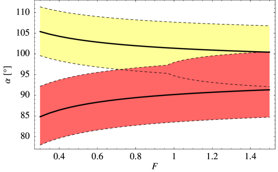
Figure 1: Dependence of $\alpha$ on $F$ for the two solutions in Table I: (1) lower band, (2) upper band. The two bands denote experimental errors from $C_{L},~{}S_{L}$ and ${\cal R}$.

The only theoretical error in our method (up to the discrete phase choice) originates in the parameter $F$. We now discuss the extraction of $\alpha$ for the entire range of $F$ given in (14), focusing on the two solutions (1) and (2) near $\alpha=\pi/2$. In Figure 1 we show the dependence of these solutions on the parameter $F$. The lower and upper solid dark lines, corresponding to solutions (1) and (2) respectively, use central values for $C_{L},~{}S_{L}$ and ${\cal R}$. The bands around these two lines give experimental errors originating in these three measurements. Focusing on the theoretical error from $F$ alone, we consider values of $\alpha$ along the dark solid lines, comparing values at $F=0.9$ with values at $F=0.3$ and $F=1.5$. We find the variation in the lower and upper solutions to be given by $(89.8^{+1.5}_{-5.0})^{\circ}$ and $(101.6^{+3.7}_{-1.2})^{\circ}$, respectively. We discard again the second solution on the basis of involving values of $\delta$ in the neighborhood of $\pi$ rather than near zero. Including the experimental error from Table I and the above theoretical uncertainty from $F$, we conclude

$$\alpha=[89.8^{+7.2}_{-6.7}~{}({\rm exp})^{+1.5}_{-5.0}~{}({\rm th})]^{\circ}~{}.$$ (35)

We note that the theoretical error, following from the range (14) in $F$ and the preference for one of the two theoretically possible solutions, is considerably smaller than the error of $11^{\circ}$ in $\alpha$ obtained from an upper bound on $|\alpha-\alpha_{\rm eff}|$ by applying the isospin triangle analysis to $B\to\rho\rho$ [7]. It is worth recapitulating the origin of this small error: Data on ${\cal R}$ implies that the penguin correction is small. Once this is established the relation $S_{L}=\sin 2\alpha$ receives only small corrections, and since $\sin 2\alpha$ is rapidly varying near $\alpha=\pi/2$ even a significant error in $S_{L}$ translates into a small error in $\alpha$.

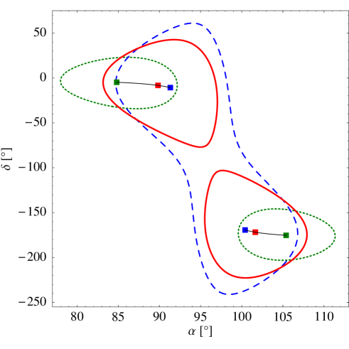
Figure 2: $\chi^{2}=1$ contours for $C_{L},~{}S_{L},~{}\mathcal{R}$ projected on the $(\alpha,\delta)$ plane. Dotted, solid and dashed curves correspond to $F=0.3,~{}0.9,~{}1.5$. The six points at focus denote the solutions for vanishing errors in $C_{L},~{}S_{L},~{}\mathcal{R}$.

In order to quantify the criterion excluding solution (2) for $\alpha$, we study now the dependence of the two solutions for $\alpha$ near $\pi/2$ on the strong phase $\delta$. In Figure 2 we plot the $\chi^{2}=1$ contours for $C_{L},~{}S_{L}$ and $\mathcal{R}$ projected on the $(\alpha,\delta)$ plane. Three different values of $F$, $F=0.3,~{}0.9,~{}1.5$, are described by the dotted, solid and dashed curves, respectively. The upper and lower parts of the curves correspond to solutions (1) and (2) discussed above. The $\chi^{2}=1$ contours of the two solutions merge because of current experimental errors. The six points of focus for the three curves, marked on two almost parallel solid segments around $\delta=-8^{\circ}$ and $\delta=-172^{\circ}$, are obtained for vanishing experimental errors in $C_{L},~{}S_{L}$ and $\mathcal{R}$. The length of the segments gives the purely theoretical uncertainty in $\alpha$ originating in the range of $F$. Figure 2 shows that when including current experimental errors in $C_{L},~{}S_{L}$ and $\mathcal{R}$ the two solutions (1) and (2) are presently distinguishable by $|\delta|<\pi/2$ and $|\delta|>\pi/2$, respectively. The additional requirement $|\delta|<\pi/2$, which excludes the second solution, will be relaxed considerably with more precise data on $C_{L}$, the error of which determines the uncertainty in $\delta$.

6. We conclude with a few comments about future improvements in the determination of $\alpha$.

1. The theoretical error in the extracted value of $\alpha$ depends weakly on the range assumed for the parameter $F$ and on the measurement of ${\cal R}$. A resolution of the disagreement between the BABAR and BELLE measurements of ${\cal R}$ will be reassuring. More precise measurements of $S_{L}$ will have direct impact on the experimental error $\pm 7^{\circ}$ on $\alpha$, while more precise measurements of $C_{L}$ will eventually reduce the phase assumption to a discrete choice. This may be compared to the isospin-method for extracting $\alpha$ from $B\to\rho\rho$, where further reduction of the error depends on what values the branching fractions will take. An intrinsic theoretical uncertainty at a level of a few degrees, caused in the isospin method by an $I=1$ final state originating from the $\rho$ width [29] and by $\rho-\omega$ mixing [30], may potentially be resolved by studying with very large statistics the dependence of $B\to 4\pi$ decay distributions on the invariant masses of pairs of pions near the $\rho$ mass.

2. Our suggestion for improving the determination of $\alpha$ replaces the application of isospin bounds in $B\to\rho\rho$ by theoretical input on the rough magnitude of $F$ and a weak assumption about the the relative strong phase between the penguin and tree amplitudes in $B^{0}\to\rho^{+}\rho^{-}$. Currently the assumption $|\delta|<\pi/2$ is required, but a weaker condition will suffice in the future. One possible test of this assumption consists of comparing globally the pattern of tree-penguin interference in $B\to\rho\rho$ and $B\to K^{*}\rho$ decays.

3. Information about $\alpha$ is also obtained from $B^{0}\to\rho^{\pm}\pi^{\mp}$ decays, which involve two ratios of penguin-to-tree amplitudes, in $B^{0}\to\rho^{+}\pi^{-}$ and $B^{0}\to\rho^{-}\pi^{+}$. SU(3) arguments relating these decays to $B\to K\rho$ and $B\to K^{*}\pi$ [31], and a calculation based on QCD factorization [18] show that these two ratios are small, in the range $0.1-0.2$, being on the smaller side in the second approach. The small ratios imply a small deviation of $\alpha$ from the value of $\alpha_{\rm eff}$ obtained in the absence of penguin amplitudes [31]. Current data for time dependence in $B^{0}\to\rho^{\pm}\pi^{\mp}$, given in terms of four observables, $C,S,\Delta C,\Delta S$ [25], imply $\alpha_{\rm eff}=(94\pm 4)^{\circ}$. An SU(3)-derived bound on the effect of penguin amplitudes, $|\alpha-\alpha_{\rm eff}|<9^{\circ}$, implies $\alpha=(94\pm 10)^{\circ}$ when adding theoretical and experimental errors in quadrature [31, 32]. A more precise determination, $\alpha=(94\pm 7)^{\circ}$, follows from the observable $S$ alone using a QCD factorization calculation for amplitudes and strong phases [18]. Both determinations require stronger assumptions than those made in this work. However, the consistency of the most precise measurements of $\alpha$ (hence, $\gamma$) is impressive, allowing us to conclude that $\alpha$ is in the vicinity of $90^{\circ}$ within a few degrees.

Acknowledgements. This work was supported in part by the Israel Science Foundation under Grants No. 1052/04 and 378/05, and by the German–Israeli Foundation under Grant No. I-781-55.14/2003. M.B. and J.R. would like to thank the Technion for its hospitality.

Note added in proof

Shortly after this paper was submitted BABAR presented the new values ${\cal B}(K^{*0}\rho^{+})=10.0\pm 1.7\pm 2.4$ and $f_{L}(K^{*0}\rho^{+})=0.53\pm 0.10\pm 0.06$ [33], so that the BABAR and BELLE results are now in very good agreement [see (31)]. The new value of ${\cal R}$ equals $0.0080\pm 0.0023$ instead of (33). This leads to the following changes in our results: Since ${\cal R}$ and $F$ enter our analysis only in the combination ${\cal R}/F$ [see (13)], the new value of ${\cal R}$ and $F=0.9$ is equivalent to the old value of ${\cal R}$ and $F=1.41$ in Figure 1. It can be seen that within current experimental errors the two solutions corresponding to (1) and (2) in Table I overlap even for $F=0.9$, i.e. the corresponding $\chi^{2}=1$ contours in Figure 2 merge also for $F=0.9$. Separating the two solutions by requiring $\delta<\pi/2$, our final result (35) now reads

$$\alpha=[91.2^{+9.1}_{-6.6}~{}({\rm exp})^{+1.2}_{-3.9}~{}({\rm th})]^{\circ}~{}.$$

The larger experimental error is due to the fact that the two solutions have merged. As discussed in the text, the forseeable improved measurement of $C_{L}$ will remedy this problem.

References

- [1] M. Kobayashi and T. Maskawa, Prog. Theor. Phys. 49, 652 (1973).
- [2] M. Gronau, Proceedings of the Tenth International Conference on Physics at Hadron Machines, Assisi, Perugia, Italy, June 20–24, 2005, Nucl. Phys. B (Proc. Suppl.) 156, 69 (2006).
- [3] J. Charles et al. [CKMfitter Group], Eur. Phys. J. C 41, 1 (2005) [hep-ph/0406184]; updated in www.slac.stanford.edu/xorg/ckmfitter.
- [4] M. Bona et al. [UTfit Collaboration], JHEP 0507, 028 (2005) [hep-ph/0501199]; updated in http://www.utfit.org.
- [5] J. Zhang et al. [BELLE Collaboration], Phys. Rev. Lett. 91, 221801 (2003) [hep-ex/0306007].
- [6] B. Aubert et al. [BABAR Collaboration], Phys. Rev. Lett. 91, 171802 (2003) [hep-ex/0307026].
- [7] B. Aubert et al. [BABAR Collaboration], Phys. Rev. Lett. 95, 041805 (2005) [hep-ex/0503049].
- [8] A. Somov et al. [Belle Collaboration], [hep-ex/0601024].
- [9] M. Gronau and D. London, Phys. Rev. Lett. 65, 3381 (1990).
- [10] Y. Grossman and H. R. Quinn, Phys. Rev. D 58, 017504 (1998) [hep-ph/9712306].
- [11] M. Gronau, D. London, N. Sinha and R. Sinha, Phys. Lett. B 514, 315 (2001) [hep-ph/0105308].
- [12] B. Aubert et al. [BABAR Collaboration], Phys. Rev. Lett. 94, 131801 (2005) [hep-ex/0412067].
- [13] M. Gronau and J. L. Rosner, Phys. Lett. B 595, 339 (2004) [hep-ph/0405173].
- [14] A. J. Buras, R. Fleischer, S. Recksiegel and F. Schwab, Nucl. Phys. B 697, 133 (2004) [hep-ph/0402112]; Eur. Phys. J. C 45, 701 (2006) [hep-ph/0512032].
- [15] M. Gronau, Phys. Rev. Lett. 63, 1451 (1989).
- [16] M. Gronau, O. F. Hernandez, D. London and J. L. Rosner, Phys. Rev. D 50, 4529 (1994) [hep-ph/9404283]; Phys. Rev. D 52, 6374 (1995) [hep-ph/9504327].
- [17] B. Aubert et al. [BABAR Collaboration], [hep-ex/0408063].
- [18] M. Beneke and M. Neubert, Nucl. Phys. B 675, 333 (2003) [hep-ph/0308039].
- [19] C. W. Chiang, M. Gronau, J. L. Rosner and D. A. Suprun, Phys. Rev. D 70, 034020 (2004) [hep-ph/0404073]. This paper contains references for earlier tests of flavor SU(3) in .
- [20] C. W. Chiang, M. Gronau, Z. Luo, J. L. Rosner and D. A. Suprun, Phys. Rev. D 69, 034001 (2004) [hep-ph/0307395].
- [21] M. Beneke, G. Buchalla, M. Neubert and C. T. Sachrajda, Phys. Rev. Lett. 83, 1914 (1999) [hep-ph/9905312].
- [22] M. Beneke, G. Buchalla, M. Neubert and C. T. Sachrajda, Nucl. Phys. B 591, 313 (2000) [hep-ph/0006124]; Nucl. Phys. B 606, 245 (2001) [hep-ph/0104110].
- [23] M. Beneke, J. Rohrer and D. Yang, [hep-ph/0512258], and in preparation.
- [24] J. Rohrer, Diploma Thesis, RWTH Aachen University (2004).
- [25] E. Barberio et al. [Heavy Flavor Averaging Group], [hep-ex/0603003].
- [26] B. Aubert et al. [BABAR Collaboration], Phys. Rev. Lett. 93, 231801 (2004) [hep-ex/0404029].
- [27] B. Aubert [BABAR Collaboration], [hep-ex/0408093].
- [28] J. Zhang et al. [BELLE Collaboration], Phys. Rev. Lett. 95, 141801 (2005) [hep-ex/0505039].
- [29] A. F. Falk, Z. Ligeti, Y. Nir and H. Quinn, Phys. Rev. D 69, 011502 (2004) [hep-ph/0310242].
- [30] M. Gronau and J. Zupan, Phys. Rev. D 71, 074017 (2005) [hep-ph/0502139].
- [31] M. Gronau and J. Zupan, Phys. Rev. D 70, 074031 (2004) [hep-ph/0407002].
- [32] M. Gronau, E. Lunghi and D. Wyler, Phys. Lett. B 606, 95 (2005) [hep-ph/0410170].
- [33] J. G. Smith, talk given at the Fourth Conference on Flavor Physics and CP Violation, Vancouver, British Columbia, Canada, April 9–12. See also http://www.slac.stanford.edu/xorg/hfag.