ITEP–PH–1–2006
New nonperturbative approach to the Debye mass in hot QCD

Abstract

The Debye mass $m_{D}$ is computed nonperturbatively in the deconfined phase of QCD, where chromomagnetic confinement is known to be present. The latter defines $m_{D}$ to be $m_{D}=c_{D}\sqrt{\sigma_{s}}$, where $c_{D}\cong 2.06$ and $\sigma_{s}=\sigma_{s}(T)$ is the spatial string tension. The resulting magnitude of $m_{D}(T)$ and temperature dependence are in good agreement with lattice calculations. Background perturbation theory expansion for $m_{D}(T)$ is discussed in comparison to standard perturbative results and recent gauge-invariant definitions.

PACS:11.10.Wx,12.38.Mh,11.15.Ha,12.38.Gc

1 Introduction

The screening of electric fields in QCD was originally considered in analogy to QED plasma, where the Debye screening mass was well understood [1], and the perturbative leading order (LO) result for QCD was obtained long ago [2], $m_{D}^{\rm(LO)}=\left(\frac{N_{c}}{3}+\frac{N_{f}}{6}\right)^{1/2}gT$. For not very large $T$, however, the purely perturbative expansion is not reliable, and attempts have been made to use the effective $3d$ theory [3, 4, 5, 6] to define the Debye mass $m_{D}$ through the coefficients, which are to be determined nonperturbatively [7]. In doing so one obtains a series [7], with the leading term of the same form as $m_{D}^{\rm(LO)}.$

The lattice calculations of $m_{D}(T)$ have been made repeatedly [8]-[15], and recently $m_{D}(T)$ was computed on the lattice for $N_{f}=0,2$ [13, 14] using the free-energy asymptotics

$$\delta F_{1}(r,T)\equiv F_{1}(r,T)-F_{1}(\infty,T)\approx-\frac{4}{3}\frac{\alpha_{s}(T)}{r}e^{-m_{D}(T)r},$$ (1)

where $F_{1}(r,T)$ was found from color singlet Polyakov loop correlator. A comparison of lattice defined $m_{D}(T)$ with $m_{D}^{\rm(LO)}$ made in [15] in the interval from $T_{c}$ up to temperatures about $5.5T_{c}$ shows that one requires a multiplicative coefficient $A_{N_{f}=0}=1.51$, $A_{N_{f}=2}=1.42$. A difficulty of the perturbative approach is that the gauge-invariant definition of the one-gluon Debye mass is not available. The purpose of our paper is to provide a gauge-invariant and a nonperturbative method, which allows to obtain Debye masses in a rather simple analytic calculational scheme. In what follows we use the basically nonperturbative approach of Field Correlator Method (FCM) [16]-[22] and Background Perturbation Theory (BPTh) for nonzero $T$ [23, 24, 25] to calculate $m_{D}(T)$ in a series, where the first and dominant term is purely nonperturbative,

$$m_{D}(T)=M_{0}+{\rm BPTh\leavevmode\nobreak\ series}.$$ (2)

Here $M_{0}$ is the gluelump mass due to chromomagnetic confinement in 3d, which is computed to be $M_{0}=c_{D}\sqrt{\sigma_{s}}$, with $\sigma_{s}(T)$ being the spatial string tension and $c_{D}\simeq 2.06$ for $N_{c}=3$. The latter is simply expressed in FCM through chromomagnetic correlator [19], and can be found either from lattice measurements of the correlator itself as in [21], or from the 3d effective theory [3]-[7], $\sqrt{\sigma_{s}}=c_{\sigma}g^{2}(T)T$, or else from the lattice data [26]. Therefore $M_{0}(T)$ is predicted for all $T$ and can be compared with lattice data [13, 14, 15], see Fig. 2.

We note, that $m_{D}(T)$ is defined here as the screening mass in the static $Q\bar{Q}$ potential $V_{1}$, which can be expressed through the gauge-invariant correlator of chromomagnetic and chromoelectric fields [21, 27, 28]. The screened Coulomb part of the potential $V_{1}$ coincides with the singlet free energy $F_{1}(r,T)$ at the leading order [29], and in what follows we shall consider also the leading order in BPTh, where the static potential $V_{1}(r)$ has a term of the same form as the r.h.s. of Eq. (1).

The paper is organized as follows. In section 2 the nonperturbative part and the perturbative BPTh series for the thermal Wilson loop are defined, and the gluelump Greens function is identified, using the path-integral formalism. In section 3 an effective Hamiltonian is derived and the first terms of expansion (2) are obtained for $m_{D}(T)$ computed through the spatial string tension $\sigma_{s}(T)$. In section 4 a comparison is made of $m_{D}(T)$ with lattice data and other approaches. Section 5 is devoted to a short summary of results and outlook.

2 Background Perturbation Theory for the thermal Wilson loop

It is well known that the introduction of the temperature for the quantum field system in thermodynamic equilibrium is equivalent to compactification along the euclidean ”time” component $x_{4}$ with the radius $\beta=1/T$ and imposing the periodic boundary conditions (PBC) for boson fields (anti-periodic for fermion ones). Thermal vacuum averages are defined in a standard way

$$\langle\ldots\rangle=\frac{1}{Z_{\beta}}\int_{\rm PBC}[DA]\ldots e^{-S_{\beta}[A]},$$ (3)

where partition function is

$$Z_{\beta}=\int_{\rm PBC}[DA]e^{-S_{\beta}[A]},\quad S_{\beta}=\int_{0}^{\beta}dx_{4}\int d^{3}xL_{YM}.$$ (4)

One starts as in [28] and [30] with the correlator of Polyakov loops $\langle L(0)L^{+}(\mbox{\boldmath${\rm r}$})\rangle$

$$L(\mbox{\boldmath${\rm x}$})\equiv\frac{1}{N_{c}}{\rm tr}P\exp(ig\int^{\beta}_{0}A_{4}(\mbox{\boldmath${\rm x}$},x_{4})dx_{4}),$$

and obtains (cf. [30]).

$$\langle L(0)L^{+}(\mbox{\boldmath${\rm r}$})\rangle=\frac{1}{N^{2}_{c}}\exp\left(-\beta F_{1}(r,\beta)\right)+\frac{N^{2}_{c}-1}{N^{2}_{c}}\exp\left(-\beta F_{8}(r,\beta)\right).$$ (5)

As it is explained in the Appendix in [27] the representation (5) can be obtained from two Polyakov loops by identical deformation of contours with tentackles meeting at some intermediate point and subsequent merging of contour into one Wilson loop using completeness relation at the meeting point $\delta_{\alpha_{1}\beta_{1}}\delta_{\alpha_{2}\beta_{2}}=\frac{1}{N_{c}}\delta_{\alpha_{1}\beta_{2}}\delta_{\alpha_{2}\beta_{1}}+2t^{a}_{\beta_{2}\alpha_{1}}t^{a}_{\beta_{1}\alpha_{2}}$, the first term contributing to the free energy $F_{1}$ of the static $Q\bar{Q}$-pair in the singlet color state, the second to the octet free energy $F_{8}$. Accordingly one ends for $F_{1}$ with the thermal Wilson loop of time extension $\beta=1/T$ and space extension $r$,

$$\exp\left(-\beta F_{1}(r,\beta)\right)=\langle W(r,\beta)\rangle=\frac{1}{N_{c}}\langle{\rm tr}P\exp(ig\int_{C}A_{\mu}dz_{\mu})\rangle.$$ (6)

Note, that in contrast to the case of the zero-temperature Wilson loop, the averaging in (6) is done with PBC applied to $A_{\mu}$, as in (3), (4).

Eq.(6) is the basis of our approach. In what follows we shall calculate however not $F_{1}$, which contains all tower of excited states over the ground state of heavy quarks $Q\bar{Q}$, but rather the static potential $V_{1}(r,T)$, corresponding to this ground state, for more details see [27].

Separating, as in BPTh [23] the field $A_{\mu}$ into NP background $B_{\mu}$ and valence gluon field $a_{\mu}$,

$$A_{\mu}=B_{\mu}+a_{\mu}$$ (7)

one can assign gauge transformations as follows

$$B_{\mu}\to U^{+}(B_{\mu}+\frac{i}{g}\partial_{\mu})U,\leavevmode\nobreak\ \leavevmode\nobreak\ a_{\mu}\to U^{+}a_{\mu}U.$$ (8)

As a next step one inserts (7) into (6) and expands in powers of $ga_{\mu}$, which gives

$$\langle W(r,\beta)\rangle=\langle W^{(0)}(r,\beta)\rangle_{B}+\langle W^{(2)}(r,\beta)\rangle_{B,a}+\ldots,$$ (9)

where according to [23] one can write $\langle\Gamma\rangle_{A}=\langle\langle\Gamma\rangle_{a}\rangle_{B}$, and $\langle W^{(2)}\rangle$ can be written as

$$\langle W^{(2)}\rangle_{B,a}=\frac{(ig)^{2}}{N_{c}}\int\langle{\rm tr}P\Phi(\prod_{xy})\langle a_{\mu}(x)a_{\nu}(y)\rangle_{a}\Phi(\coprod^{xy})\rangle_{B}dx_{\mu}dy_{\nu}.$$ (10)

Here $\Phi(\prod)$ and $\Phi(\coprod)$ are parallel transporters along the pieces of the original Wilson loop $W(r,\beta)$, which result from the dissection of the Wilson loop at points $x$ and $y$, see Fig.1. Thus the Wilson loop $W^{(2)}(r,\beta)$ is the standard loop $W^{(0)}(r,\beta)$ augmented by the adjoint line connecting points $x$ and $y$. It is easy to see using (8), that this construction is gauge invariant.

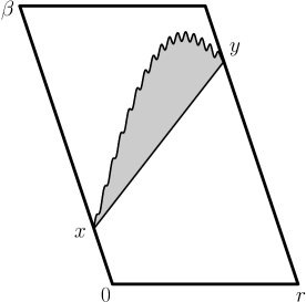
Figure 1: The gluon trajectory (wavy line) and the adjoint surface $S_{gl}^{H}$ (dark region) attached to the thermal Wilson loop.

For OGE propagator one can write the path integral Fock-Feynman-Schwinger (FFS) representation for nonzero $T$ as in [23]

$$G_{\mu\nu}(x,y)=\langle a_{\mu}(x)a_{\nu}(y)\rangle_{a}=$$

$$=\int^{\infty}_{0}ds\int(D^{4}z)^{w}_{xy}\exp(-K)\Phi^{adj}(C_{xy})\left(P_{F}\exp(2ig\int^{s}_{0}F_{\sigma\rho}(z(\tau))d\tau)\right)_{\mu\nu},$$ (11)

$$\Phi^{adj}(C_{xy})=P\exp(ig\int_{C_{xy}}B_{\mu}dz_{\mu}),$$

where the open contour $C_{xy}$ runs along the integration path in (11) from the point $x$ to the point $y$ as shown Fig.1, and $K=\frac{1}{4}\int^{s}_{0}(\dot{z}_{\mu})^{2}d\tau$. The path integration measure $(D^{4}z)^{w}_{xy}$ is given by

$$(D^{4}z)_{xy}^{w}=\prod^{N}_{k=1}\frac{d^{4}\Delta z(k)}{(4\pi\varepsilon)^{2}}\int\frac{d^{4}p}{(2\pi)^{4}}\sum^{+\infty}_{n=-\infty}\exp\left({ip_{\mu}\left(\sum^{N}_{k=1}\Delta z_{\mu}(k)-(x-y)_{\mu}-n\beta\delta_{\mu 4}\right)}\right)$$ (12)

with $N\varepsilon=s$ and $\Delta z_{\mu}(k)=z_{\mu}(k)-z_{\mu}(k-1)$. Thus, $(D^{4}z)_{xy}^{w}$ is a path integration with boundary conditions $z_{\mu}(\tau=0)=x_{\mu}$ and $z_{\mu}(\tau=s)=y_{\mu}$ (this is marked by the subscript $xy$) and with all possible windings in the Euclidean temporal direction (this is marked by the superscript $w$).

We must now average over $B_{\mu}$ the geometrical construction obtained by inserting (11) into (10), i.e.

$$\langle\Phi(\prod_{xy})\Phi^{adj}(C_{xy})\Phi(\coprod^{xy})\rangle_{B}\equiv\langle W_{xy}(r,\beta)\rangle_{B}.$$ (13)

One can apply to (10) the nonabelian Stokes theorem, and to this end one has to fix the surface bounded by the rectangular $r,\beta$ with the adjoint line passing on the surface. The standard prescription of the minimal surface valid for the fixed boundary contours, in our case when chromoelectric confinement is missing and only spatial projections of the surface enter, leads to the deformation of the original plane surface due to gluon propagation, consisting of this original surface plus the additional adjoint surface $S_{gl}^{H}$ connecting gluon trajectory with its projection on the plane $(r,\beta)$, see Fig.1, where this projection is simplified to be the straight line. The nonabelian Stokes theorem yields the area law [16, 17] for distances $r\gg\lambda_{g}$, $\lambda_{g}-$ gluon correlation length, $\lambda_{g}\sim 0.2$ fm

$$\langle W_{xy}(r,\beta)\rangle_{B}=\exp(-\sigma^{E}S_{\rm plane})\exp(-\sigma^{E}_{adj}S^{E}_{gl}-\sigma_{adj}^{H}S_{gl}^{H}),$$ (14)

where $S^{E,H}_{gl}$ are projections of gluon-deformed piece of surface $S_{gl}$ into time-like, space-like surfaces respectively.

For $T>T_{c}$ one has $\sigma^{E}\equiv 0$ and one obtains exactly the form containing the gluelump Green’s function

$$\langle W^{(2)}\rangle_{B,a}={(ig)^{2}}C_{2}(f)\int^{\beta}_{0}dx_{4}\int^{\beta}_{0}dy_{4}G_{44}(r,t_{4}),$$ (15)

where $t_{4}\equiv x_{4}-y_{4}$, $C_{2}(f)=(N_{c}^{2}-1)/2N_{c}$ and $G_{44}(r,t_{4})$ is

$$G_{44}(r,t_{4})=\int^{\infty}_{0}ds\int(D^{4}z)_{xy}^{w}\exp(-K)\exp(-\sigma_{adj}^{H}S_{gl}^{H}).$$ (16)

In (16) we have neglected the last exponent on the r.h.s. of (11), which produces spin-dependent terms found small in [31], for more discussion see Appendix 4 of [32].

Thus the gluon Green’s function in the confined phase becomes a gluelump Green’s function, where the adjoint source trajectory is the projection of the gluon trajectory on the Wilson loop plane.

Now in the deconfined phase, $T\geq T_{c}$, where, magnetic confinement takes place in spatial coordinates, so that one can factorize as follows $(G_{\mu\nu}(x,y)\equiv\delta_{\mu\nu}G(x,y))$

$$G(x,y)=\int^{\infty}_{0}ds\int(Dz_{4})^{w}_{x_{4}y_{4}}(Dz_{3})_{x_{3}y_{3}}G^{(2)}(0,0;s)\exp\left({-\frac{1}{4}\int^{s}_{0}(\dot{z}^{2}_{3}+\dot{z}^{2}_{4})d\tau}\right),$$ (17)

where $G^{(2)}(0,0;s)$ is the 2d Green’s function with $s$ playing the role of time and interaction given by the area law term, $\exp(-\sigma_{adj}^{H}S_{gl}^{H})$. Here $S_{gl}^{H}$ is the Nambu-Goto expression

$$S_{gl}^{H}=\int^{s}_{0}d\tau\int^{1}_{0}d\beta\sqrt{\dot{w}^{2}_{i}w_{k}^{{}^{\prime}2}-(\dot{w}_{i}w^{\prime}_{i})^{2}},$$ (18)

and $w_{i}=z_{i}(\tau)\beta,\leavevmode\nobreak\ \leavevmode\nobreak\ i=1,2,\leavevmode\nobreak\ \leavevmode\nobreak\ w^{\prime}_{i}=\frac{\partial w_{i}}{\partial\beta},\leavevmode\nobreak\ \leavevmode\nobreak\ \dot{w}_{i}=\frac{\partial w_{i}}{\partial\tau}$.

In (17) one can specify coordinates in such a way, that $x_{4}=0,y_{4}=t_{4},x_{3}=0,y_{3}=r$ and $x_{1,2}=y_{1,2}$.

For $G^{(2)}$ one can write

$$G^{(2)}(0,0;s)=\int(Dz_{1})_{00}(Dz_{2})_{00}\exp\left({-\frac{1}{4}\int^{s}_{0}(\dot{z}^{2}_{1}+\dot{z}^{2}_{2})d\tau-\sigma_{adj}^{H}S_{gl}^{H}}\right).$$ (19)

The path integral (19) can be expressed through the Hamiltonian $H^{(2)}$, which is obtained from the Euclidean action

$$A=\int^{s}_{0}d\tau\mathcal{L}(z_{i},\dot{z}_{i})=\frac{1}{4}\int^{s}_{0}(\dot{z}^{2}_{1}+\dot{z}^{2}_{2})d\tau+\sigma_{adj}^{H}S_{gl}^{H}$$ (20)

$$G^{(2)}(x,y;s)=\langle x|\exp({-H^{(2)}s})|y\rangle$$ (21)

It is easy to derive, that $G^{(2)}(0,0;s)\equiv G^{(2)}(s)$ behaves at small and large $s$ as

$$G^{(2)}(s\to 0)\propto\frac{1}{4\pi s};\leavevmode\nobreak\ \leavevmode\nobreak\ G^{(2)}(s\to\infty)\propto M^{2}_{0}\exp({-M^{2}_{0}s}),$$ (22)

where $M^{2}_{0}$ is the lowest mass eigenvalue of $H^{(2)}$. As an explicit example one can consider a rather realistic case when interaction term $\sigma_{adj}^{H}S_{gl}^{H}$ in (19) is replaced by the oscillator term

$$\sigma_{adj}^{H}S_{gl}^{H}\to\frac{1}{4}\int^{s}_{0}d\tau\bar{\omega}^{2}z^{2}_{i}(\tau)$$

and one obtains

$$G^{(2)}_{osc}(s)=\frac{\bar{\omega}}{4\pi\sinh\bar{\omega}s},\leavevmode\nobreak\ \leavevmode\nobreak\ \bar{\omega}=M^{2}_{0}$$ (23)

One can see that asymptotic behaviour (22) is satisfied provided that $\bar{\omega}=M_{0}^{2}$. On the other hand, the eigenvalues of $H^{(2)}$ (when the role of time is played by $s$), $M_{n}^{2}$ can be expressed through $\tilde{M}^{2}_{n}$, where $\tilde{M}_{n}$ are eigenvalues of gluelump Hamiltonian $\tilde{H}^{(2)}$ when Eucledian time evolution is chosen along $z_{3}$. Those will be found in the next section. Since $d\tau={dz_{3}}/{2\mu},\leavevmode\nobreak\ \leavevmode\nobreak\ dz_{3}\equiv dt$ and $\tilde{M}_{n}=2\mu_{n}$, the Hamiltonian $\int H^{(2)}d\tau=\int({H^{(2)}}/{2\mu})dz_{3}=\int\tilde{H}^{(2)}dz_{3}$ and one has the equality $M^{2}_{n}\cong\tilde{M}^{2}_{n}$ with the accuracy of $\sim 5\%$ known for the einbein technic calculations [24].

Calculating $(Dz_{3})_{0r}$ one has

$$\int(Dz_{3})_{0r}\exp\left(-\frac{1}{4}\int^{s}_{0}\dot{z}_{3}^{2}d\tau\right)=\frac{1}{\sqrt{4\pi s}}\exp\left(-\frac{r^{2}}{4s}\right).$$ (24)

A similar calculation with $(Dz_{4})^{w}_{ot_{4}}$ yields

$$\int(Dz_{4})^{w}_{ot_{4}}\exp\left(-\frac{1}{4}\int^{s}_{0}\dot{z}_{4}^{2}d\tau\right)=\frac{1}{\sqrt{4\pi s}}\sum^{+\infty}_{n=-\infty}\exp\left(-\frac{(t_{4}+n\beta)^{2}}{4s}\right),$$ (25)

and combining all terms one has

$$G(r,t_{4})=\frac{C_{2}(f)g^{2}}{16\pi^{2}}\int^{\infty}_{0}\frac{ds}{s^{2}}\tilde{G}^{(2)}(s)\sum^{+\infty}_{n=-\infty}\exp\left({-\frac{[(t_{4}+n\beta)^{2}+r^{2}]}{4s}}\right),$$ (26)

where we have defined $\tilde{G}^{(2)}(s)\equiv 4\pi sG^{(2)}(0,0;s)$ so that $\tilde{G}^{(2)}(s\to 0)\to 1,\leavevmode\nobreak\ \leavevmode\nobreak\ \tilde{G}^{(2)}(s\to\infty)\to\exp(-M^{2}_{0}s)$.

We are now in the position to obtain the screened static (color Coulomb) potential. Indeed, identifying in the lowest order in $O(g^{2})$ in (6), (15), (16), (26), one has

$$F_{1}(r,\beta)=V_{1}^{(1)}(r,\beta)=-C_{2}(f)g^{2}\int^{\frac{\beta}{2}}_{-\frac{\beta}{2}}dt_{4}G(r,t_{4}),$$ (27)

which can be rewritten using (26) as

$$V_{1}^{(1)}(r,\beta)=-\frac{C_{2}(f)g^{2}}{16\pi^{2}}\int^{\infty}_{0}\frac{ds}{s^{2}}\exp\left({-\frac{r^{2}}{4s}}\right)\chi(s,\beta)\tilde{G}^{(2)}(s),$$ (28)

where $\chi(s,\beta)$

$$\chi(s,\beta)=\int^{\frac{\beta}{2}}_{-\frac{\beta}{2}}dt_{4}\sum^{+\infty}_{n=-\infty}\exp\left(-\frac{(t_{4}+n\beta)^{2}}{4s}\right).$$ (29)

Now for large $\beta$ (small $T$), $\beta\gg r,\beta M_{0}\gg 1$, one can keep in the sum (29) only the term $n=0$, which yields $\chi_{n=0}(s,\beta)=\sqrt{4\pi s}$. From (28) one then can conclude that $s\sim r^{2}$, and for $r^{2}M^{2}_{0}\sim sM_{0}^{2}\gg 1$ one can replace $\tilde{G}^{(2)}(s)$ by the asymptotics, $\tilde{G}^{(2)}(s)\cong\exp(-M^{2}_{0}s)$, which yields

$$V_{1}^{(1)}(r,T)=-\frac{C_{2}(f)\alpha_{s}}{r}e^{-M_{0}r},\leavevmode\nobreak\ \leavevmode\nobreak\ rT\ll 1.$$ (30)

In the opposite limit of small $\beta$ (large $T$), $\beta\ll r$, one can use the following relation [33] for the sum in (29)

$$\sum^{+\infty}_{n=-\infty}\exp\left(-\frac{(t_{4}+n\beta)^{2}}{4s}\right)={\frac{\sqrt{4\pi s}}{\beta}}\sum^{+\infty}_{k=-\infty}\exp\left({-{\frac{4\pi^{2}k^{2}}{\beta^{2}}}s+i{\frac{2\pi k}{\beta}}t_{4}}\right),$$ (31)

which yields for $\chi(s,\beta),$

$$\chi(s,\beta)=\sqrt{4\pi s}\left(1+O(e^{-{{4\pi^{2}k^{2}s}/{\beta^{2}}}})\right)$$ (32)

and hence the screened color Coulomb potential $V_{1}^{(1)}(r,T)$ has the form (30) also at $rT\gg 1$. We shall assume accordingly that (30) holds for all temperatures and distances $r\geq\lambda_{g}$ in the order $O(\alpha_{s})$, and the next section will be devoted to the calculation of $M_{0}$.

3 Nonperturbative Debye mass

As it was argued in the previous section, the screened gluon propagator is actually the gluelump Green’s function, defined in (16). In this section we shall calculate the gluelump spectrum and hence the set of Debye masses. This problem is similar to the calculation of the so-called meson and glueball screening masses, which was done analytically in [25], and in our present case we must compute the gluelump screening masses. Below we shall heavily use the glueball calculation of [25], simplifying it to the case, when one of the gluon masses is going to infinity–thus yielding a gluelump.

We note, that the role of time is played by the coordinate $z_{3}$, (when the third axis passes through the positions of $Q$ and $\bar{Q}$).

So we write $z_{3}\equiv t_{3},\leavevmode\nobreak\ \leavevmode\nobreak\ 0\leq t_{3}\leq r$, and define transverse vector $\mbox{\boldmath${\rm z}$}_{\perp}=(z_{1},z_{2})$ and $z_{4}(t_{3})$. Introducing the einbein variable $\mu$ [34], one has

$$\frac{dz_{3}}{d\tau}=2\mu,\leavevmode\nobreak\ \leavevmode\nobreak\ 0\leq\tau\leq s;\leavevmode\nobreak\ \leavevmode\nobreak\ K=\frac{1}{2}\int^{r}_{0}dt_{3}\mu(t_{3})(1+\dot{}\mbox{\boldmath${\rm z}$}^{2}_{\perp}+\dot{z}^{2}_{4})$$ (33)

and $G(x,y)$ acquires the form

$$G(x,y)=\int D\mu\int(D^{2}z_{\perp})_{00}(Dz_{4})^{w}_{xy}\exp(-A),$$ (34)

where the action is

$$A=K+\sigma^{H}_{adj}S^{H}_{gl}$$ (35)

Proceeding as in [25] one arrives to the effective Hamiltonian representation

$$G(x,y)=\langle x|\sum_{n}\exp({-H_{n}r})|y\rangle,$$ (36)

with the temperature-dependent Hamiltonian $(r_{\perp}\equiv|\mbox{\boldmath${\rm z}$}_{\perp}|)$

$$H_{n}=\sqrt{\mbox{\boldmath${\rm p}$}^{2}_{\perp}+(2n\pi T)^{2}}+\sigma_{adj}^{H}r_{\perp}.$$ (37)

The spatial gluelump masses are to be found from the eigenvalues of the equation

$$H_{n}\varphi^{(n)}_{k}=M^{(n)}_{K}\varphi_{k}^{(n)}.$$ (38)

and for $n=0$ the Hamiltonian (37) has the form

$$H_{0}=\sqrt{\mbox{\boldmath${\rm p}$}^{2}_{\perp}}+\sigma_{adj}^{H}r_{\perp}$$ (39)

or in the form with einbein variables which will be useful for discussion

$$H_{0}^{\rm einb}=\frac{\mbox{\boldmath${\rm p}$}^{2}_{\bot}}{2\mu}+\frac{\mu}{2}+\sigma_{adj}^{H}r_{\perp}=\frac{\mbox{\boldmath${\rm p}$}^{2}_{\perp}}{2\mu}+\frac{\mu}{2}+\frac{{\sigma_{adj}^{H}}^{2}r^{2}_{\perp}}{2\nu}+\frac{\nu}{2}.$$ (40)

The OGE potential, $\Delta V=-3\alpha_{s}^{\rm eff}/r$, will be considered as the small correction. Note the difference between two-dimensional distance $r_{\perp}$ entering in the spatial protection of the area in the gluelump Wilson loop, $S_{gl}^{H}$, and the $3d$ distance $r$ entering in the $3d$ color Coulomb interaction in $\Delta V$. The eigenvalue of (40), $H_{0}^{\rm einb}\varphi=\varepsilon_{0}\varphi$, with $\alpha_{s}^{\rm eff}=0$ is

$$\varepsilon_{0}(\mu,\nu)=\frac{\mu+\nu}{2}+\frac{\sigma_{adj}^{H}}{\sqrt{\mu\nu}}$$ (41)

and the minimization in $\mu,\nu$ implied in the einbein formalism [34] yields

$$\varepsilon_{0}(\mu_{0},\nu_{0})=2\sqrt{\sigma_{adj}^{H}}=3\sqrt{\sigma_{s}},$$ (42)

where $\sigma_{s}$ is the fundamental spatial string tension and $\sigma_{adj}^{H}=(9/4)\sigma_{s}$ for $SU(3)$.

One can compare this value with more exact one, obtained from solution of the differential equation in (40) and to this end one can use the eigenvalue of the screening glueball mass found in [25], (which is larger by a factor of $\sqrt{2}$ than that of our gluelump mass, cf. Eq. (44) of [25] and our Eq. (39)). In this way one obtains

$$\varepsilon_{0}=2.82\sqrt{\sigma_{s}}$$ (43)

which differs from (42) by 6%.

In the next approximation the OGE potential for the gluelump comes into play. Here one should take into account that the gluon-gluon OGE interaction acquires a large NLO correction, which strongly reduces the LO result as it is seen in the BFKL calculation (see discussion in [35]), and therefore the effective value of $\alpha_{s}^{\rm eff}$ is smaller than in the $Q\bar{Q}$ interaction. Specifically, in the gluelump mass calculation at $T=0$ [31] the mass of the lowest gluelump for $\alpha_{s}^{\rm eff}=0$ is $M=1.4$ GeV, and it decreases to $M\approx 1$ GeV, when $\alpha_{s}^{\rm eff}=0.15$. This latter value of $M$ is in agreement with lattice correlator calculations [21]; the same situation takes place in the glueball mass calculation [35], where also $\alpha_{s}^{\rm eff}\cong 0.15$ and we shall adopt it in our Eq. (40). The correction of $\varepsilon_{0}$ due to $\alpha_{s}^{\rm eff}$ in the lowest order is easily computed using (40); as a result one has $\Delta\varepsilon_{0}=-(9/\sqrt{\pi})\alpha_{s}^{\rm eff}\sqrt{\sigma_{s}}\approx-5.08\alpha_{s}^{\rm eff}\sqrt{\sigma_{s}}$. As a final result we write the Debye mass (lowest gluelump mass $M_{0}\equiv m_{D}$) for $\alpha_{s}^{\rm eff}=0.15$

$$m_{D}=\varepsilon_{0}+\Delta\varepsilon_{0}=(2.82-5.08\alpha_{s}^{\rm eff})\sqrt{\sigma_{s}}\cong 2.06\sqrt{\sigma_{s}}$$ (44)

4 Numerical results and discussion

One can now compare our prediction for $m_{D}(T)=c_{D}\sqrt{\sigma_{s}(T)}$ with the latest lattice data [15]. The spatial string tension is chosen in the form [26, 36]

$$\sqrt{\sigma_{s}(T)}=c_{\sigma}g^{2}(T)T,$$ (45)

with the two-loop expression for $g^{2}(T)$

$$g^{-2}(t)=2b_{0}\ln\frac{t}{L_{\sigma}}+\frac{b_{1}}{b_{0}}\ln\left(2\ln\frac{t}{L_{\sigma}}\right),\leavevmode\nobreak\ \leavevmode\nobreak\ \leavevmode\nobreak\ t\equiv\frac{T}{T_{c}}$$ (46)

where

$$b_{0}=\left(\frac{11}{3}N_{c}-\frac{2}{3}N_{f}\right)\frac{1}{16\pi^{2}},\leavevmode\nobreak\ \leavevmode\nobreak\ \leavevmode\nobreak\ b_{1}=\left(\frac{34}{3}N_{c}^{2}-(\frac{13}{3}N_{c}-\frac{1}{N_{c}})N_{f}\right)\frac{1}{(16\pi^{2})^{2}}.$$

The measured in [26] spatial string tension in pure glue QCD corresponds to the values of $c_{\sigma}=0.566\pm 0.013$ and $L_{\sigma}\equiv\Lambda_{\sigma}/T_{c}=0.104\pm 0.009.$ On the left panel of Fig. 2 are shown lattice data [26] and the theoretical curve (solid line) for $T/\sqrt{\sigma_{s}(T)}$ calculated according to (45) with $c_{\sigma}=0.564,L_{\sigma}=0.104$ and $N_{f}=0$.

Figure 2: Left panel: The temperature over the square root of the spatial string tension versus $T/T_{c}$ for pure glue QCD. Solid line corresponds to Eq.(45). The lattice data are from [26]. Right panel: Chromoelectric Debye mass $m_{D}/T$ for 2-flavor QCD (upper lines) and quenched ($N_{f}=0$) QCD (lower lines) versus $T/T_{c}$. Solid lines are calculated using $m_{D}(T)=2.09\sqrt{\sigma_{s}(T)}$, where $\sqrt{\sigma_{s}(T)}$ corresponds to Eq.(45) with $N_{f}=2$ for upper solid line and $N_{f}=0$ for lower solid line. Dashed lines are calculated using Eq.(47), $N_{f}=2$–upper line, $N_{f}=0$–lower line. The lattice data are from [13].

On the right panel of Fig. 2 are shown lattice data [13] and theoretical curves for the Debye mass in quenched ($N_{f}=0$) and 2-flavor QCD. Solid lines correspond to our theoretical prediction, $m_{D}(T)=c_{D}\sqrt{\sigma_{s}(T)}$, with $c_{D}=2.09$ and for $\sqrt{\sigma_{s}(T)}$ we exploit the same parameter ($c_{\sigma}=0.564,L_{\sigma}=0.104$) as in the left panel. The upper solid line is for the Debye mass in 2-flavor QCD, and the lower – for quenched QCD. We note that in computing $m_{D}(T)$ using (45), (46) all dependence on $N_{f}$ enters only through the Gell-Mann–Low coefficients $b_{0}$ and $b_{1}$. For comparison we display in the right panel of Fig. 2 dashed lines for $m_{D}(T)/T$, calculated with a perturbative inspired ansatz [15]

$$m_{D}^{Latt}(T)=A_{N_{f}}\sqrt{1+\frac{N_{f}}{6}}g(T)T.$$ (47)

Quenched QCD corresponds to $A_{N_{f}=0}=1.51$ and $L_{\sigma}^{N_{f}=0}=1/(1.14\cdot 2\pi)$ [15], and for the 2-flavor QCD $A_{N_{f}=2}=1.42$ and $L_{\sigma}^{N_{f}=2}=1/(0.77\cdot 2\pi)$ [15].

Let us now consider higher orders of BPTh for $m_{D}$. From the gauge-invariant expansion (9) one obtains the next term $\langle W^{(4)}(r,\beta)\rangle$, which contains the double gluon propagator $\langle a_{\mu_{1}}(x_{1})a_{\mu_{2}}(x_{2})a_{\nu_{1}}(y_{1})a_{\nu_{2}}(y_{2})\rangle_{a}$ in the background field of the Wilson loop, which is proportional to $g^{4}(T)$. One can show that the background averaging of this propagator attached to the Wilson loop yields the diagram of the exchange of a double gluon gluelump between $Q$ and $\bar{Q}$, and therefore the NLO BPTh Debye mass will coincide with the double gluon gluelump mass, computed for $T=0$ in [31] analytically and in [38] on the lattice. As a result the lightest $2g$ gluelump mass appeared to be 1.75 times heavier than the lightest $1g$ gluelump mass. We expect therefore that also at $T>T_{c}$ the same ratio of masses takes place, so that the asymptotics of gluon (gauge-invariant and background-averaged) gluon exchanges in BPTh has the form [23, 39]

$$V^{GE}(r,T)=-\frac{4}{3}\frac{\alpha_{s}^{(0)}}{r}e^{-m_{D}^{(1gl)}(T)r}-\frac{c_{2}(r)(\alpha_{s}^{(0)})^{2}}{r}e^{-m_{D}^{(2gl)}(T)r}+\ldots,$$ (48)

where $c_{2}(r)$ contains the asymptotic freedom logarithm.

One can see in (48) that the second term on the r.h.s. is subleading and small as compared to the first one, both due to $(\alpha_{s}^{(0)})^{2}$ and due to higher mass of $m_{D}^{(2gl)}$. At this point it is essential to note that this second term should enter as a sum over all possible $2g$ gluelumps. In one particular case, when two gluons form a color singlet, they decouple from the plane surface of the Wilson loop and create a $2g$ glueball, coupled by the spatial string (see Fig.3). The corresponding glueball mass is computed in [25] and is 1.7 times larger than the LO BPTh mass (44), which is denoted as $m_{D}^{(1gl)}(T)$ in (48). It is interesting that the aforementioned glueball mass corresponds to the gauge-invariant Debye mass suggested in [40], and as seen in (48) it appears in the NLO BPTh, giving a small correction to the LO Debye screening potential. Therefore one can identify the Debye mass $m_{D}\equiv m_{D}^{(1gl)}$ with the accuracy $O(\alpha_{s}^{(0)}e^{-\Delta m_{D}r})$ where $\Delta m_{D}=m_{D}^{(2gl)}-m_{D}^{(1gl)}\geq 0.6GeV$.

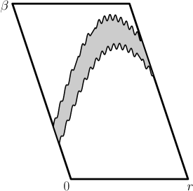
Figure 3: NLO BPTh contribution to the Debye screening potential from the $2g$ glueball exchange

The consideration above was done for the chromoelectric Debye mass, which appears in the screening Coulomb potential in the temporal plane $(4i)$ appearing due to the $G_{44}(x,y)$ gluelump Green’s function. One can similarly consider exchange of ”magnetic gluon” by insertion of the magnetic field vertex $F_{ik}\sim D_{i}a_{k}-D_{k}a_{i}$ into the Wilson or Polyakov loops. This vertex automatically appears in the Green’s function from the term $\propto\exp(g\sigma_{\mu\nu}\int^{s}_{0}F_{\mu\nu}d\tau)$ creating spin-dependent interaction. The same procedure as above leads to the ”magnetic gluelump” Green’s function, which differs from the ”electric gluelump” case by the nonzero gluelump momentum $L=1$. The corresponding mass is easily obtained as in (43), giving

$$\varepsilon_{L}(\mu_{0},\nu_{0})=2\sqrt{(1+L+2n_{r})\sigma_{adj}},\leavevmode\nobreak\ \leavevmode\nobreak\ \varepsilon_{1}=\sqrt{2}\varepsilon_{0}\approx 4\sqrt{\sigma_{s}}.$$

Thus nonperturbative magnetic Debye mass is $\sqrt{2}$ times heavier than the electric one.

5 Conclusions

We have studied Debye screening in the hot nonabelian theory. For that purpose the gauge-invariant definition of the free energy of the static $Q\bar{Q}$-pair in the singlet color state was given in terms of the thermal Wilson loop. Due to the chromomagnetic confinement persisting at all temperatures $T$, the hot QCD is essentially nonperturbative. To account for this fact in a gauge-invariant way the BPTh was developed for the thermal Wilson loop using path-integral FFS formalism. As a result one obtains from the thermal Wilson loop the screened Coulomb potential with the screening mass corresponding to the lowest gluelamp mass. Applying the Hamiltonian formalism to the BPTh Green’s functions with the einbein technic the gluelump mass spectrum was obtained. As a result, we have derived the leading term of the BPTh for the Debye mass which is the purely nonperturbative, $m_{D}(T)=c_{D}\sqrt{\sigma_{s}(T)}$ with $c_{D}\approx 2.06$.

Comparison of our theoretical prediction (solid lines on the right panel Fig. 2) with the perturbative-like ansatz (47) (dashed lines) shows that both agree reasonably with lattice data in the temperature interval $T_{c}<T\leq 5T_{c}$; the agreement is slightly better for our results. At the same time, in (47) a fitting constant is used $A_{N_{f}}\sim 1.5$, which is necessary even at $T/T_{c}\sim 5$. At this point one can discuss the accuracy and approximations of our approach. As it was checked in numerous applications to hadron masses and wave function (see review [17]) the accuracy of the Hamiltonian technic is around $(5\div 7)$%, while the area law is as accurate for loop sizes beyond $\lambda_{g}\sim 0.2$ fm. At smaller distances the area law in (16), (19) is replaced by the ”area squared” expression [16] which yields effectively much smaller $m_{D}(T)$. Therefore we expect that the Debye regime (1) with the $m_{D}$ as in (44) starts at $r\geq\lambda_{g}\approx 0.2$ fm. As a whole we expect the accuracy of the first approximation of our approach, Eq. (44) to be better than 10%, taking also into account the bias in the definition of $\alpha_{s}^{\rm eff}$ for the gluelump. The temperature region near $T_{c}$ needs additional care because i) the behaviour (45) deviates from the data (see left panel of Fig. 2) and ii) contribution of chromoelectric fields above $T_{c}$ (correlator $D_{1}^{E}$, see [27]) which was neglected above. Both points can be cured and will be given elsewhere.

The authors are grateful to Frithjof Karsch for supplying us with numerical data, useful remarks and fruitful discussion with one of the authors (Yu.S). Our gratitude is also to M.A.Trusov for help and useful advices.

The work is supported by the Federal Program of the Russian Ministry of Industry, Science, and Technology No.40.052.1.1.1112, and by the grant of RFBR No. 06-02-17012, and by the grant for scientific schools NS-843.2006.2.

References

- [1] I.Akhiezer and S.Peletminski, ZhETF 38 (1960) 1829; J.-P.Blaizot, E.Iancu and R.Parwani, Phys. Rev. D52 (1995) 2543.
- [2] E.Shuryak, ZhETF 74 (1978) 408: J.Kapusta, Nucl. Phys. B 148 (1979) 461; D.Gross, R.Pisarski and L.Yaffe, Rev. Mod. Phys. 53 (1981) 43.
- [3] P.Ginsparg, Nucl. Phys. B 170 (1980) 388; T.Appelquist and R.Pisarski, Phys. Rev. D23 (1981) 2305; S.Nadkarni, Phys. Rev. D27 (1983) 917.
- [4] K.Kajantie, K.Rummukainen and M.Shaposhnikov, Nucl. Phys. B407 (1993) 356; K.Kajantie, M.Laine, K.Rummukainen and M.Saposhnikov, Nucl. Phys. B458 (1996) 90.
- [5] E.Braaten and A.Nieto, Phys. Rev. D 51 (1995) 6990; Phys. Rev. D 53 (1996) 3421.
- [6] M.E.Shaposhnokov, hep-ph/9610247.
- [7] K.Kajantie, M.Laine, K.Rummukainen and M.Shaposhnikov, Nucl.Phys. B503 (1997) 357; K.Kajantie, et al., Phys.Rev.Lett. 79 (1997) 3130.
- [8] U.Heller, F.Karsch and J.Rank, Phys. Rev. D57 (1998) 1438.
- [9] O.Kaczmarek, F. Karsch, E.Laermann and M.Lutgemeier, Phys. Rev. D62 (2000) 034021.
- [10] S.Digal, S.Fortunato and P.Petreczky, Phys. Rev. D68 (2003) 034008.
- [11] A.Nakamura and T.Saito, Prog. Theor. Phys. III (2004) 733.
- [12] O.Kaczmarek, F. Karsch, P.Petreczky and F.Zantow, Phys. Rev. D70 (2004) 074505.
- [13] O.Kaczmarek and F.Zantow, Phys. Rev. D71 (2005) 114510.
- [14] M.Döring, S.Ejiri, O.Kaczmarek, F. Karsch and E.Laermann, hep-lat/0509150.
- [15] O.Kaczmarek and F.Zantow, hep-lat/0512031.
-
[16]
H.G.Dosch, Phys. Lett. B 190(1987) 177;
H.G.Dosch and Yu.A.Simonov, Phys. Lett. B 205 (1988) 339;
Yu.A.Simonov, Nucl. Phys. B 307 (1988) 512. - [17] A.Di Giacomo, H.G.Dosch, V.I.Shevchenko, Yu.A.Simonov, Phys. Rept. 372 (2002) 319.
- [18] Yu.A.Simonov, in: Proc. of the Intern.School of Physics, E.Fermi, Varena, 1995; IOS Press, 1996; hep-ph/9509404.
- [19] Yu.A.Simonov, JETP Lett. 54(1991) 249 .
- [20] Yu.A.Simonov, JETP Lett. 55 (1992) 605.
-
[21]
A.Di Giacomo and H.Panagopoulos, Phys. Lett. B285 (1992) 133;
M.D’Elia, A.Di Giacomo, and E.Meggiolaro, Phys. Lett. B408 (1997) 315;
A.Di Giacomo, E.Meggiolaro and H.Panagopoulos, Nucl. Phys. B483 (1997) 371;
M.D’Elia, A.Di Giacomo, and E.Meggiolaro, Phys. Rev. D67 (2003) 114504;
G.S.Bali, N.Brambilla, A.Vairo, Phys. Lett. B 42 (1998) 265;
E.Meggiolaro, Phys. Lett. B451 (1999) 414. - [22] N.O.Agasian, Phys. Lett. B562 (2003) 257.
-
[23]
Yu.A.Simonov, Phys. At. Nucl. 58 (1995) 309;
N.O.Agasian, JETP Lett. 57 (1993) 208; JETP Lett. 71 (2000) 43. - [24] Yu.A.Simonov, J.A.Tjon, Ann. Phys. 228 (1993) 1; ibid 300 (2002) 54.
- [25] E.L.Gubankova and Yu.A.Simonov, Phys. Lett. B360 (1995) 93.
- [26] G.Boyd et al., Nucl. Phys. B 469 (1996) 419.
- [27] Yu.A.Simonov, Phys. Lett. B 619 (2005) 293.
- [28] A.Di Giacomo, E.Meggiolaro, Yu.A.Simonov, A.I.Veselov, hep-ph/0512125.
- [29] P.Petreczky, Eur. Phys. J. C43 (2005) 51.
-
[30]
L.G.Mc Lerran, B.Svetitsky, Phys. Rev. D24 (1981) 450;
S.Nadkarni, Phys. Rev. D33 (1986), ibid D34 (1986) 39904. - [31] Yu.A.Simonov, Nucl. Phys. B592 (2001) 350.
- [32] Yu.A.Simonov, Phys. Atom Nucl. (in press), hep-ph/0501182.
- [33] D.Mamford, ”Tata Lectures on theta I“, Birkhauser, Boston, 1983.
- [34] A.Dubin, A.B.Kaidalov, Yu.A.Simonov, Phys. Lett. B323 (1994) 41; Yad. Fiz. 56 (1993) 213.
- [35] A.B.Kaidalov, Yu.A.Simonov, Phys. Lett. B477 (2000) 163; Phys. Atom. Nucl. 63 (2000) 1428; hep-ph/0512151.
- [36] F.Karsch, E.Laermann, M.Lutgemeier, Phys. Lett. B346 (1995) 94.
- [37] N.O.Agasian and K.Zarembo, Phys. Rev. D57 (1998) 2475.
- [38] M.Foster, C.Michael, Phys. Rev. D59 (1999) 094509.
- [39] Yu.A.Simonov, Phys. Atom. Nucl. 58 (1995) 107.
- [40] P.Arnold and L.G.Yaffe, Phys. Rev. D52 (1995) 7208.